A Control-Oriented ANFIS Model of Evaporator in a 1-kWe Organic Rankine Cycle Prototype

Abstract

This paper presents a control-oriented neuro-fuzzy model of brazed-plate evaporators for use in organic Rankine cycle (ORC) engines for waste heat recovery from exhaust-gas streams of diesel engines, amongst other applications. Careful modelling of the evaporator is both crucial to assess the dynamic performance of the ORC system and challenging due to the high nonlinearity of its governing equations. The proposed adaptive neuro-fuzzy inference system (ANFIS) model consists of two separate neuro-fuzzy sub-models for predicting the evaporator output temperature and evaporating pressure. Experimental data are collected from a 1-kWe ORC prototype to train, and verify the accuracy of the ANFIS model, which benefits from the feed-forward output calculation and backpropagation capability of the neural network, while keeping the interpretability of fuzzy systems. The effect of training the models using gradient-descent least-square estimate (GD-LSE) and particle swarm optimisation (PSO) techniques is investigated, and the performance of both techniques are compared in terms of RMSEs and correlation coefficients. The simulation results indicate strong learning ability and high generalisation performance for both. Training the ANFIS models using the PSO algorithm improved the obtained test data RMSE values by 29% for the evaporator outlet temperature and by 18% for the evaporator outlet pressure. The accuracy and speed of the model illustrate its potential for real-time control purposes.

1. Introduction

The internal combustion (IC) engine is the main technology currently used in the transportation sector. A typical IC engine converts about 40% of the fuel combustion energy into useful work. Legislation on vehicle emission continues to become more stringent to reduce the impact of IC engines on the environment. To this end, technologies—such as gasoline direct injection (GDI) [1], turbo direct injection (TDI) [2], and fuel stratified injection (FSI) [3]—have been developed and implemented in recent years to increase the efficiency of IC engines. Despite the advantages of such technologies, the thermal efficiency of IC engines needs to be improved to meet regulatory targets such as those agreed upon at the COP21 in the legally binding Paris Agreement, which is set to reduce greenhouse gas emissions. Recently, new methods of waste heat recovery (WHR) have been explored to utilise the significant amount of energy that is released to the atmosphere from the exhaust and coolant of IC engines [4]. The objective is to convert this waste thermal energy into useful mechanical or electrical energy. Several viable WHR technologies can be used to harness this waste thermal energy, such as turbo-compound, thermoelectric generators, piezoelectric generators, and organic Rankine cycle (ORC) engines. Among them, ORC systems are the preferred method of WHR in IC engines due to their low manufacturing cost and high efficiency. WHR technologies can contribute to enhancing the overall conversion efficiency of IC engines [5,6,7].

ORCs are a promising WHR technology that has been widely considered in many industries due to their features such as simplicity and high efficiency. The ORC is a heat-engine thermodynamic cycle that exhibits the potential to be deployed for recovery of waste heat in IC engines, the exhaust gases of which are an unsteady heat source with fluctuating temperature and mass flow rate [8,9]. Key characteristics of the ORC engine that make it a desirable solution for waste heat recovery in IC engines include modularity, versatility, and technological maturity of components (due to the similarities with the refrigeration systems). Moreover, ORC systems are able to recover waste heat in the low- to medium-temperature range. Most current investigations on ORCs are focused on theoretical and thermodynamic analysis [10], cycle optimisation [11], techno-economic optimisation [12,13], and working fluid selection [14]. In particular, combined fluid-design optimisation studies explore the potential of novel working fluids using computer aided molecular design (CAMD) techniques [15,16,17]. Several studies also propose advanced off-design optimisation algorithms to maximise the performance of an ORC engine operating under variable heat-source conditions [18,19,20,21].

However, the latter are based on quasi-steady models of the ORC engine and are thus not suitable for dynamic applications. For safe and successful implementation of ORCs in the automotive industry, a reliable and precise control scheme is required to ensure the safe operation of the engine, prevent organic fluid decomposition, and reduce the risk of component damage. Furthermore, designing a reliable control algorithm for the ORC in the mobile applications depends on accurate modelling of all the components within the cycle. The heat exchanges (i.e., evaporator and condenser) are key components of the ORC system as they are responsible for a large share of the overall exergy destruction [22] (heat transfer over a finite temperature difference being irreversible by nature) and are challenging to model due to the high nonlinearity of their governing equations. In addition, the dynamic behaviour of ORC engines is governed by the large thermal inertia of the heat exchangers, in particular by that of the evaporator, which has a direct impact on the response time of an ORC engine subject to fluctuations in heat-source conditions (namely, temperature and mass flowrate). Therefore, an accurate model of the evaporator is required to capture the dynamics of the system and is of prominent importance, not only because it is necessary for cycle optimisation and working fluid selection, but also as it allows a comprehensive optimisation of the dynamic control strategy.

Evaporator models available in the literature can be categorised into three main categories, namely: finite volume (FV) models, moving boundary (MB) models, and intelligent based models such as fuzzy and neural network models [23,24,25]. As illustrated in Figure 1, FV models are based on a spatial discretisation of the evaporator into a finite number of equally spaced control volumes, with the thermo-physical properties of the working fluid considered constant within each control volume. For this modelling technique, a higher number of control volumes results in an increased precision but significantly increases the computational complexity. Therefore, a trade-off must be made between accuracy and processing time to select the adequate spatial resolution of FV models [26]. FV techniques are computationally expensive and are thus appropriate for performance assessment and working fluid selection, but cannot be applied to high-frequency, real-time control purposes.

By contrast, MB models are control-oriented models based on a fixed spatial discretisation of the evaporator into three regions (liquid, two-phase mixture, vapour), the size of which varies with time. The MB technique results in a slight improvement in computational complexity, however, models developed by this technique cannot tolerate nonexistence of the distinct phases of the working fluid. Therefore, this technique is not suitable for situations such as start-up or shut-down because of the resulting singularity in numerical problems [23]. Evaporator fuzzy models have been developed recently to improve the real-time calculation speed of the models [24,28]; however, setting the rules for identifying the model based on the available data is a time-consuming task. Another approach for developing an agile model of the evaporator is the neuro-fuzzy technique. Neuro-fuzzy models are data-driven techniques that require training before implementation. As opposed to predictive methods, which require an iterative solution, neuro-fuzzy models are much faster and can be utilised for control purposes. Adaptive neuro-fuzzy inference system (ANFIS) is an intelligent modelling technique acquiring the modelling benefits of Sugeno fuzzy inference system and pattern recognition ability of feedforward neural network [29]. Khosravi et al. [30] used ANFIS-PSO algorithm for thermodynamic modelling of geothermal based ORC equipped with solar system. Authors, in previous studies [27,31], have developed ANFIS models based on the available data from FV evaporator models that offer reduced complexity, high accuracy and lower computational burden for prediction of the working-fluid and heat-source outlet temperatures. This paper investigates the application of neuro-fuzzy techniques for modelling a plate evaporator using time-resolved high-fidelity experimental data obtained on a 1-kWe ORC prototype.

This paper is structured as follows: Section 2 describes the layout and operation of the 1-kWe ORC testing facility. In Section 3, the architecture of the ANFIS model and the node functions within its layers are discussed for a fuzzy inference system with two inputs and one output. Two methods are introduced in Section 4 for training the ANFIS model and limitations and advantages of both methods are pointed out. In Section 5, data collection and application of the ANFIS method for modelling the evaporator outlet temperature and pressure in the testing facility are discussed. The simulation results and discussions of the study are presented in Section 6. The simulation tests are designed to evaluate the effectiveness of the proposed modelling technique. Finally, the paper closes by summarising and discussing key conclusions from this work in Section 7.

2. ORC System Layout and Test Bench Prototype

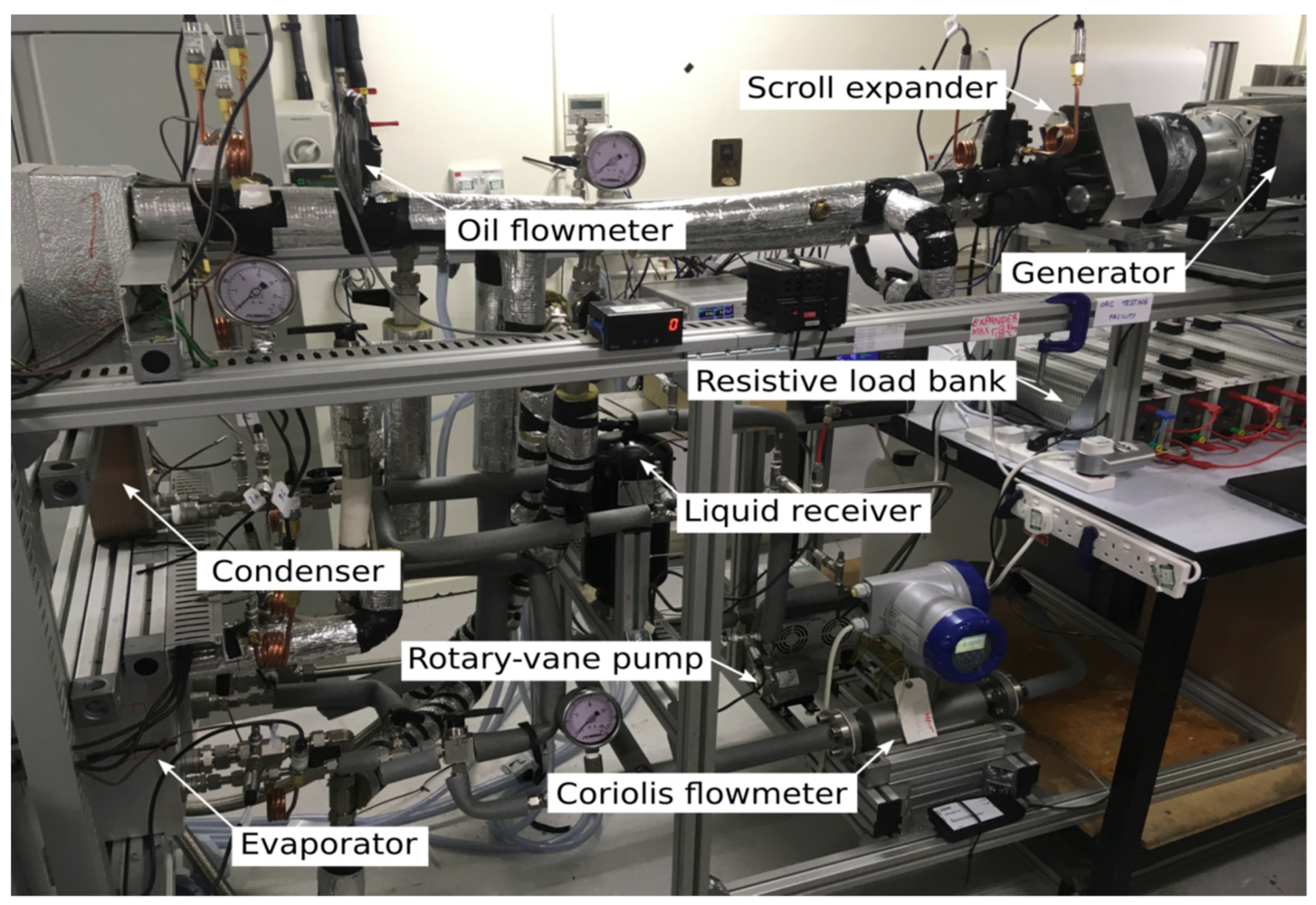
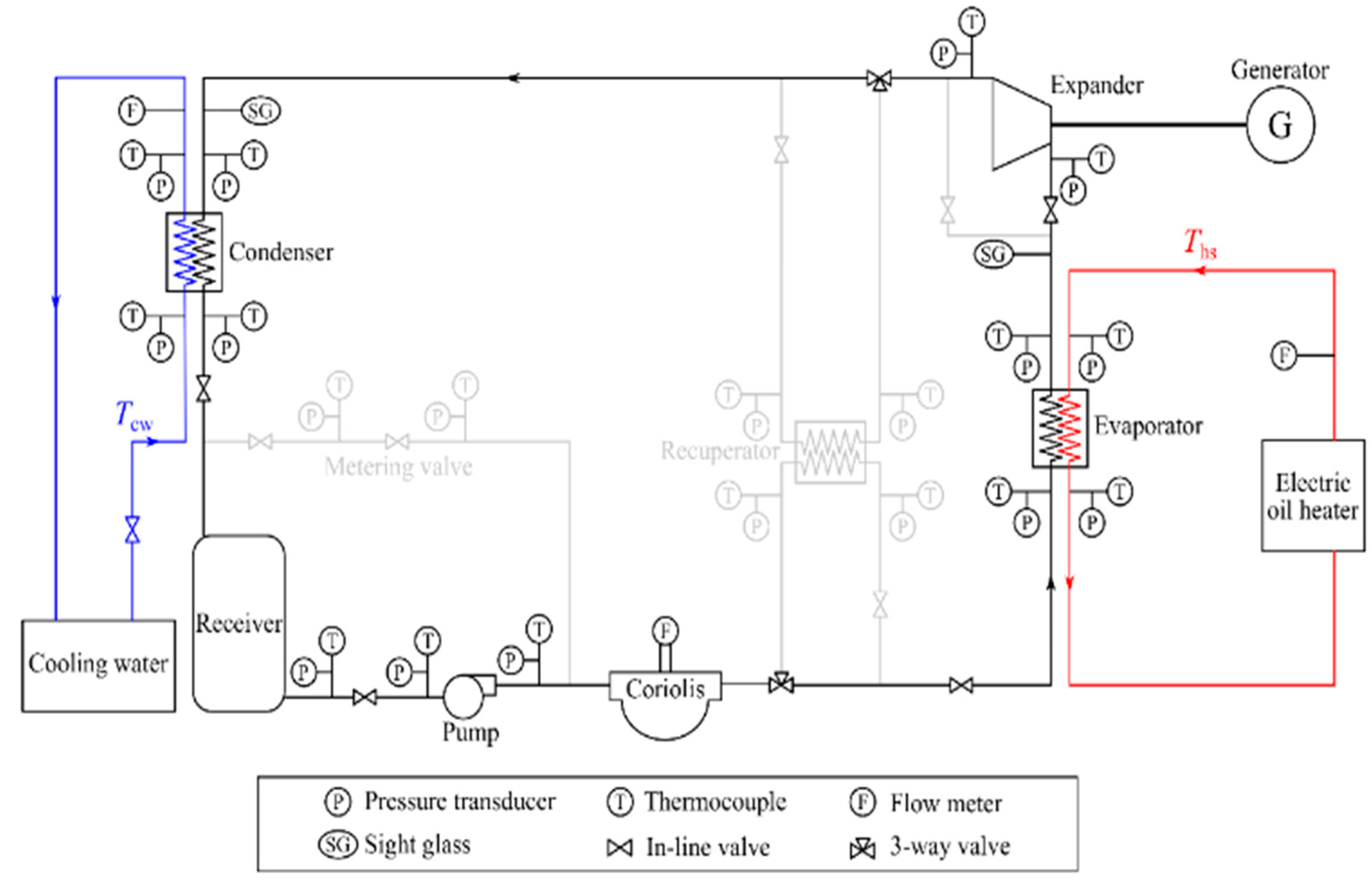
The testing facility, commissioned at the Clean Energy Processes (CEP) Laboratory at Imperial College London, comprises a rotary-vane pump, brazed-plate evaporator and condenser, and a scroll expander coupled magnetically to a generator with an adjustable resistive load. The ORC prototype is operated with R245fa as the working fluid, which can maintain above-atmospheric pressure within the condenser and prevent non-condensable air from leaking into the closed loop. The rotary-vane pump circulates the organic fluid through the cycle and allows adjustment of the flowrate. Shaft power is produced from the expansion of the high-temperature, high-pressure vapour exiting the evaporator down to the low pressure maintained in the condenser. The generator converts the expander shaft mechanical work into electrical energy, which is dissipated within a resistive load bank made of a set of adjustable resistors – with an equivalent overall resistance ranging from 10 to 60 Ω. This resistive load bank is able to dissipate safely up to 2 kW of heat without external ventilation and allows to control the torque applied to the expander shaft. The low-pressure vapour leaving the expander is then cooled down and fully condensed in the water-cooled condenser. To avoid cavitation in the pump and maintain zero subcooling at the condenser outlet, a liquid receiver is placed between the condenser and the pump. An 18-kW electric oil heater with adjustable delivery temperature is used as the heat source for the ORC prototype, thus providing a controllable stream of hot Marlotherm SM oil. A detailed piping and instrumentation diagram (P&ID) of the testing facility is shown in Figure 2 and an actual picture of the test bench is presented in Figure 3.

As shown in Figure 2, pressure transducers and thermocouples (T-type) are placed at the inlet and outlet of each component to monitor the working fluid state throughout the cycle and provide high-fidelity measurements of the components and system performance. A DAQ970A data acquisition system is used to record time-resolved experimental data from the apparatus with a 1/2-Hz sampling rate. Detailed specifications of the key ORC components are listed in

Table 1. Components specification of the ORC test prototype [32].

	Fluid Name	Mass Flowrate	Temperature Range
Heat-source thermal fluid	Marlotherm SM oil	0.01–1.4 kg/s	93–142 °C
Working fluid	R254fa	14–58 g/s	7–136 °C
Cooling fluid	Water	0.4 kg/s	18 °C
	Model	Type	Area	Specifications
Pump	TMFR2 (Fluid-o-Tech, Italy)	Magnet-driven rotary vane pump	-	1100–3000 RPM
Condenser	CB60-30H-F (Alfa Laval, Sweden)	Brazed-plate	1.62 m2	-
Evaporator	B12Lx18 (SWEP, UK)	Brazed-plate	0.45 m2	-
Expansion machine	E15H22N4.25 (Air Squared, USA)	Scroll expander	-	14.5 cm3/rev, 1kWe
	Model
Data acquisition system	DAQ970A (Keysight Technologies, UK)
Pressure transducers	PXM309 (Omega Engineering, UK)
Coriolis flowmeter	Optimass 6000 (Krohne, UK)

.

3. Architecture of an Adaptive Neuro-Fuzzy Inference System (ANFIS)

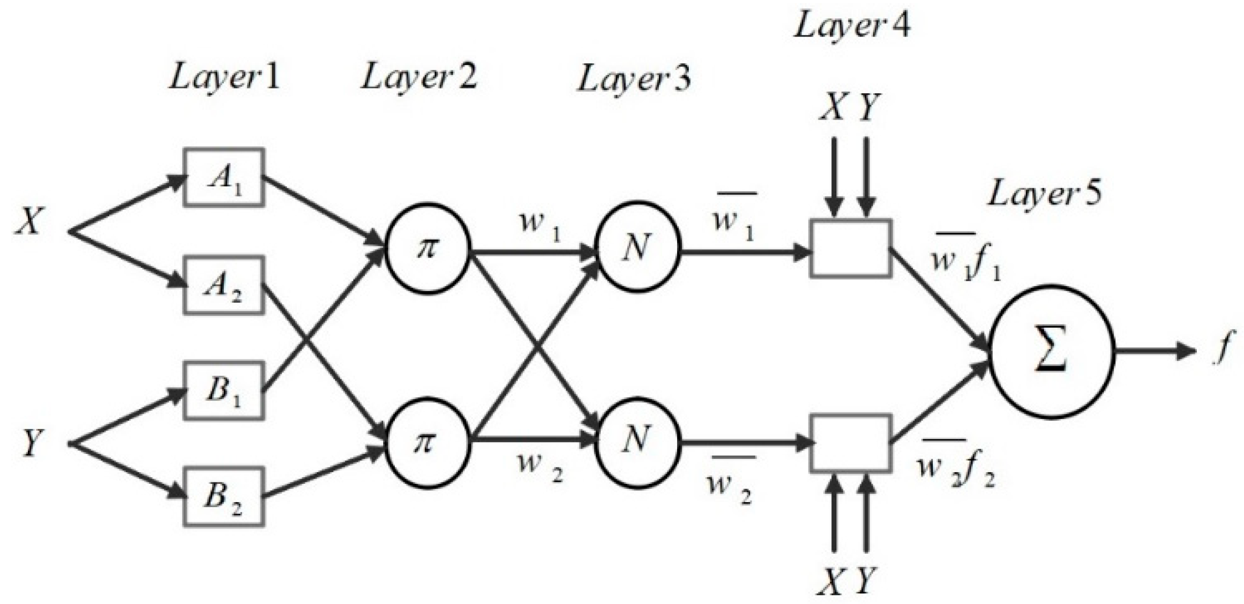
ANFIS is as an advanced method widely used to model and control complex engineering systems [29]. An ANFIS network is able to extract non-linear relationships of complex multivariable problems using modelling benefits of Sugeno fuzzy inference system and pattern recognition power of feedforward neural networks by means of learning with training data. The advantage of this method compared with other similar methods, such as ANN, is the interpretability in terms of linguistic variables [33]. Because of its fuzzy logic capabilities, ANFIS models are not considered as pure black-box models, and therefore are more interpretable [33]. Moreover, ANFIS is an adequate compromise between neural network and fuzzy system providing smoothness and adaptability for the model [34]. Consequently, the model is able to handle uncertainties better and is less sensitive to noise. The ANFIS architecture comprises five layers. Each layer contains some adaptive or fixed nodes which are connected using directional links to form the network. Fixed nodes are performing a specific task while the output of adaptive nodes depends on the parameters incorporated in their node function. The learning rule specifies how these parameters should change to minimise a prescribed error function [29].

To avoid complexity, a FIS with two inputs and one output is assumed in describing the ANFIS architecture. In the rule base of FIS two TSK rules are considered as follows:

$$\begin{array}{ll}\mathbf{Rule\; 1:}& \begin{array}{l}\mathrm{if} x \mathrm{is} A_1 \mathrm{is} B_1, \mathrm{then}:\\ f_1=p_{1}x+q_{1}y+r_1;\end{array}\\ \mathbf{Rule\; 2:}& \begin{array}{l}\mathrm{if} \mathrm{is} A_2 \mathrm{is} B_2, \mathrm{then}:\\ f_2=p_{2}x+q_{2}y+r_2,\end{array}\end{array}$$

(1)

where x and y denote the input variables and $f_i$ is the output. $A_i$ and $B_i$ are demarcated over the input domain and are regarded as the fuzzy sets. $p_i$, $q_i$, and $r_i$ are regarded as the linear polynomial parameters in the fourth layer of ANFIS network. Figure 4 represents the architecture of the ANFIS network, formed by implementing these two rules. The square and circle node symbols are deployed to illustrate the adaptive and fixed nodes, respectively. The node function for layers 1 to 5 of this architecture are as follows:

Layer 1:

The nodes in the first layer of ANFIS are parameterised membership functions and the parameters set in this layer are referred to as premise parameters. These nodes are adaptive and can represent various types of membership functions such as triangular, trapezoidal, generalised bell and Gaussian. In case of the Gaussian shape membership function, the node function is

$$\begin{array}{ll}{O}_{1, i}={\mu }_{A_i}\left(x\right)& \mathrm{for} i=1, 2; \mathrm{or}\\ O_{1, i}={\mu }_{B_{i-2}}\left(y\right)& \mathrm{for} i=3, 4.\end{array}$$

(2)

A and B denote the linguistic labels, x and y represent the inputs to the node i and μ(x) and μ(y) are Gaussian membership functions ranging from 0 to 1, as follows:

$$\mu \left(x\right)=\exp \left(-\frac{{\left(C_i-x\right)}^2}{2{\sigma }_i{}^2}\right) ,$$

(3)

where $c_i$ determine the centre and ${\sigma }_i$ represent the fuzzy set width. The training cost is determined using the number of training parameters, thus, since Gaussian membership function has only two adjustable parameters it is the most frequently used membership function in the literature [35]. In this study, Gaussian membership function is adopted for partitioning the input space because of its features such as fewer tuneable parameters and smooth representation of the domain.

Layer 2:

Nodes in the second layer are fixed and labelled as π. In this layer, the output of nodes is obtained by multiplying all incoming signals. The node output ascertains the firing strength of the rules, as:

$$O_{2,i}=w_i={\mu }_{A_i}\left(x\right){\mu }_{B_i}\left(y\right) \mathrm{for} i=1, 2.$$

(4)

Layer 3:

The fixed nodes in this layer are labelled as N. The normalised firing strengths is obtained by dividing the firing strength of ith rule to sum of all rules firing strengths:

$${\overline{w}}_i=\frac{w_i}{w_1+w_2} \mathrm{for} i=1, 2.$$

(5)

Layer 4:

The nodes in the fourth layer have three adjustable parameters and hence are regarded as adaptive nodes. Their node function is calculated as:

$$O_{4,i}={\overline{w}}_i{f}_i={\overline{w}}_i\left(p_{i}x+q_{i}y+r_i\right) ,$$

(6)

where ${\overline{w}}_i$ is the normalised firing strength, and $p_i$, $q_i$ and $r_i$ are referred to as consequent parameters, which are identified during the training process of the network.

Layer 5:

The single node in this layer is a fixed node and is labelled as Σ. The crisp output of this layer is calculated by adding all of the incoming signals as

$$O_{5,1}={{\displaystyle \sum }}_i{\overline{w}}_i{f}_i=\frac{{{\displaystyle \sum }}_i{w}_i{f}_i}{{{\displaystyle \sum }}_i{w}_i} .$$

(7)

4. Learning Algorithm of ANFIS

The aim of training the ANFIS network is to adjust the premise and consequent parameters in the adaptive nodes to minimise a performance measure known as the error function. Despite outperforming other fuzzy methods, ANFIS requires an effective learning algorithm for training the parameters of the network. In the original ANFIS paper proposed by Jang [29] a hybrid gradient descent, least square estimate (GD-LSE) method is used to identify the premise and consequent parameters of the network. In this method, because of utilising a gradient-based approach, the algorithm has a tendency to trap in local minima. Therefore, in search for a more effective training method for ANFIS, metaheuristic approaches have been investigated by researchers as an alternative for identifying the network parameters. Extensive literature review illustrates that various metaheuristic algorithms—such as PSO, GA, ABC, and their variants—have been used for training the premise and consequent parameters of the ANFIS network for a range of engineering problems.

Table 2. Summary of studies based on metaheuristic algorithms for ANFIS training.

	Premise	Consequent
Shoorehdeli, Teshnehlab [36]	AWPSO	FFRLS
Shoorehdeli, Teshnehlab [37]	AWPSO	EKF
Sargolzaei et al. [38]	PSO	PSO
Turki, Bouzaida [39]	PSO	PSO
Rini, Shamsuddin [40]	PSO	PSO
Karaboga, Kaya [41]	ABC	ABC
Soto, Melin [42]	GA	LSE
Cardenas, Garcia [43]	GA	GA

summarises some studies which have used metaheuristic methods for training the ANFIS network.

In this study, among many methods of minimising the performance measure, the particle swarm optimisation (PSO) and standard gradient descent, lest square estimate (GD-LSE) are chosen to train the ANFIS network. Moreover, their performance for matching training and test datasets is compared. The root mean square error (RMSE) is selected as the main performance indicator. The network output will better match the training target as the RMSE approaches zero.

4.1. GD-LSE Algorithm

In the architecture of the aforementioned ANFIS network, layer 1 and layer 4 contain adjustable parameters that need to be tuned for the network to match the training data. The least square estimate can be utilised to find the optimal values for the consequent parameters; however, since the premise parameters are not fixed, the search space becomes too large and it affects the convergence speed adversely. Therefore, by using a hybrid approach GD-LSE algorithm can speed up the process of training the network. The hybrid GD-LSE comprises a forward and a backward pass to train consequent and premise parameters, respectively.

Table 3. Two-pass parameter identification of the GD-LSE method.

Parameter	Forward Pass	Backward Pass
Antecedent parameters	Fixed	Gradient decent
Consequent parameters	Least square estimate	Fixed
Signals	Node outputs	Error signals

illustrates this two-pass algorithm for identifying the premise and consequent parameters of the model.

The data is presented to the network after fixing the premise parameters. The node outputs propagate forward through the network and, consequently, the network output is obtained as a linear combination of consequent parameters as:

$$f=\frac{w_1}{w_1+w_2}{f}_1+\frac{w_2}{w_1+w_2}{f}_2={\overline{w}}_1{f}_1+{\overline{w}}_2{f}_2.$$

(8)

Substituting the fuzzy if-then rules into Equation (8) yields:

$$f=\left({\overline{w}}_{1}x\right)p_1+\left({\overline{w}}_{1}y\right)q_1+\left({\overline{w}}_1\right)r_1+\left({\overline{w}}_{2}x\right)p_2+\left({\overline{w}}_{2}y\right)q_2+\left({\overline{w}}_2\right)r_2.$$

(9)

Equation (9) is linear in the consequent parameters $p_1, q_1, r_1, p_2, q_2$ and $r_2$, and can thus be written as:

$$f=XW,$$

(10)

and, if the X matrix is invertible:

$$W=X^{-1}f.$$

(11)

Otherwise, W is calculated by deploying a pseudo-inverse as:

$$W={(X^{T}X)}^{-1}{X}^{T}f,$$

(12)

where $X^T$ is the transpose of $X$, and ${(X^{T}X)}^{-1}{X}^T$ is the pseudo-inverse of$X$ if $X^{T}X$ is non-singular. However, $X^{T}X$ may become singular during the iterations that makes the problem ill-defined. Moreover, although Equation (12) is concise in notation finding the inverse of X is expensive in computation. Therefore, to overcome this issue the recursive LSE method proposed by Jang [29] can be employed as:

$$W_{i+1}=W_i+S_{i+1}{x}_{i+1}\left(f_{i+1}^T-x_{i+1}^T{W}_i\right) \mathrm{with} i=0, 1, \dots , P-1;$$

(13)

$$S_{i+1}=S_i-\frac{S_i{x}_{i+1}{x}_{i+1}^T{S}_i}{1+x_{i+1}^T{S}_i{x}_{i+1}} ,$$

(14)

where $S_i$ is the covariance matrix and least square estimate of $W$ is equal to $W_P$. $x_i^T$ is the ith row vector of matrix $X$ and $f_i^T$ is the ith element of $f$.

After identifying the consequent parameters, the output of network can be calculated and the error measure of the $n^{th}$ entery of the training data can be obtained as:

$$E_n={\left(T_n-O_n\right)}^2$$

(15)

where $T_n$ and $O_n$ represent the desired output and ANFIS output, respectively. Therefore, the RMSE of the whole training dataset can be computed as follows:

$$RMSE=\sqrt{\sum \frac{E_n}{n}}$$

(16)

In the backwards pass, the consequent parameters are fixed and the error signals propagate through the network in the reverse direction. Accordingly, using the GD algorithm, the premise parameters located in the first layer of the network are updated as:

$$c_{ij}\left(t+1\right)=c_{ij}\left(t\right)-\frac{\eta }{p}\cdot \frac{\partial E}{\partial c_{ij}},$$

(17)

where, $c_{ij}$ is the membership function’s adjustable parameter and $\eta$ represents the learning rate. To obtain the partial derivative,$\frac{\partial E}{\partial c_{ij}}$, the chain rule is applied as:

$$\frac{\partial E}{\partial c_{ij}}=\frac{\partial E}{\partial f}\cdot \frac{\partial f}{\partial f_i}\cdot \frac{\partial f_i}{\partial w_i}\cdot \frac{\partial w_i}{\partial {\mu }_{ij}}\cdot \frac{\partial {\mu }_{ij}}{\partial c_{ij}}.$$

(18)

4.2. Particle Swarm Optimisation

PSO is an iterative metaheuristic computational algorithm inspired by social behaviour of birds and fishes within a flock. This method is first proposed by Eberhart and Kennedy and is considered as one of the swarm intelligence population-based search methods that is usually exploited to solve optimisation problems [44]. In PSO algorithm, potential solutions to the optimisation problem are referred to as particles. In each iteration, the position and velocity of the particles are updated by moving them in the search domain. Each particle movement is determined using its local best position ($x_{\mathrm{P},\mathrm{best}}$) but is influenced by the other particles best-known position in the search-space ($x_{\mathrm{G},\mathrm{best}}$) as

$$v_i\left(k\right)=w{v}_i\left(k-1\right)+{\rho }_1\left(x_{\mathrm{P},\mathrm{best}}-x_i\left(k\right)\right)+{\rho }_2\left(x_{\mathrm{G},\mathrm{best}}-x_i\left(k\right)\right)$$

(19)

$$x_i\left(k\right)=x_i\left(k-1\right)+v_i\left(k\right)$$

(20)

where ${\rho }_1$ and ${\rho }_2$ are random variables defined as ${\rho }_1=r_1{c}_1$ and ${\rho }_2=r_2{c}_2$, with $r_1$ and $r_2$ ~ $U\left(0, 1\right)$. The variables $c_1$ and $c_2$ are positive acceleration constants that satisfy the condition $c_1+c_2\le 4$ [45]. $w$ is the inertial weight and is determined using the inertial weight approach (IWA) as follows [46]:

$$w=w_{\max }-\frac{w_{\max }-w_{\min }}{N_{\mathrm{itr},\max }} N_{\mathrm{itr}}$$

(21)

where $w_{\max }$ and $w_{\min }$ are the initial and final weights, respectively, $N_{\mathrm{itr}}$ is the current iteration number, and $N_{\mathrm{itr},\max }$ denotes the maximum number of iterations.

In the original GD-LSE method proposed by Jang [29], convergence of parameters is dependent on their initial value. Since this method is a gradient based approach the convergence speed of the algorithm is quite slow, especially for problems with a large set of variables. Furthermore, setting the best learning rate in the backpropagation algorithm is not an easy task and requires trial and error.

The PSO algorithm does not use the gradient of the optimisation problem as opposed to the classic optimisation methods such as GD-LSE. Therefore, it does not require the optimisation problem to be differentiable, however it cannot guarantee convergence to an optimal solution. Moreover, for a determined size of network, training ANFIS using the PSO algorithm is favourable as it is less computationally expensive [37].

5. Data Collection and Model Implementation

In this experiment, for modelling the evaporator, a set of 756 input-output data pairs are collected from the ORC testing facility by varying the heat source mass flow rate and temperature and working fluid mass flow rate. For the heat source, the mass flow rate and temperature of the supplied Marlotherm SM oil stream is altered using the electric heater in the range of 0.01 to 1.37 kg/s and 93 to 142 °C, respectively. Mass flow rate of the working fluid is also altered in the range of 14.4 to 57.8 g/s by manually changing the pump speed. Four separate multi-input single-output sub-models are trained for prediction of evaporator output temperature ($T_{\mathrm{r},\mathrm{out}}$) and evaporator output pressure ($P_{\mathrm{r},\mathrm{out}}$). The inputs to sub-models are identical and consist of mass flow rate of heat source (${\dot{m}}_{\mathrm{h}}$), temperature of heat source ($T_{\mathrm{h}}$) and mass flow rate of the working fluid (${\dot{m}}_{\mathrm{r}}$). The recorded outputs for the sub-models are the evaporator outlet temperature ($T_{\mathrm{r},\mathrm{out}}$) and evaporator outlet pressure ($P_{\mathrm{r},\mathrm{out}}$). For evaluating the models, the data set is randomly divided to two subsets of training data set and test data set. The ANFIS network is optimised using the training data set whereas the test data set which is deployed for evaluating the model. In sub-models, 70% of data points are used for training the network and the remaining data points are deployed to test the constructed network. Among the available methods of clustering, fuzzy c-means (FCM) algorithm, due to its high flexibility is used for clustering the input space and generating the base FIS. The GD-LSE and PSO techniques are applied as the learning algorithm to optimise the base FIS. The training parameters for all four sub-models are listed in

Table 4. Summary of R coefficients obtained for the evaporator outlet temperature sub-model.

Parameters	GD-LSE ANFIS Model for ${\mathit{T}}_{\mathbf{r}\mathbf{,}\mathbf{o}\mathbf{u}\mathbf{t}}$	GD-LSE ANFIS Model for ${\mathit{P}}_{\mathbf{r}\mathbf{,}\mathbf{o}\mathbf{u}\mathbf{t}}$	PSO ANFIS Model for ${\mathit{T}}_{\mathbf{r}\mathbf{,}\mathbf{o}\mathbf{u}\mathbf{t}}$	PSO ANFIS Model for ${\mathit{P}}_{\mathbf{r}\mathbf{,}\mathbf{o}\mathbf{u}\mathbf{t}}$
Training dataset samples	529 × 4	529 × 4	529 × 4	529 × 4
Test dataset samples	227 × 4	227 × 4	227 × 4	227 × 4
Clustering method	FCM	FCM	FCM	FCM
Membership functions	Gaussian	Gaussian	Gaussian	Gaussian
Number of clusters	8 × 3	8 × 3	8 × 3	8 × 3
Number of epochs	1000	1000	-	-
Number of linear parameters	32	32	32	32
Number of nonlinear parameters	48	48	48	48
Total number of parameters	80	80	80	80
Number of fuzzy rules	8	8	8	8
Maximum iteration	-	-	1000	1000
Population size	-	-	80	80
Inertial weight	-	-	1	1
$\mathrm{Personal} \mathrm{learning} \mathrm{coefficient} (C_1$)	-	-	1	1
$\mathrm{Global} \mathrm{learning} \mathrm{coefficient} (C_2$)	-	-	2	2

. The performance of both training methods is compared in terms of the RMSE and linear correlation coefficient (R) for both sub-models.

6. Results and Discussion

Two neuro-fuzzy models of evaporator are developed to predict the evaporator outlet temperature and evaporator outlet pressure in a 1-kWe ORC test rig. Figure 5 represents the comparison between evaporator outlet temperature prediction in the models trained using GD-LSE and PSO techniques. As illustrated in Figure 5, for the training dataset, RMSE of 3.5 and 2.4 achieved for GD-LSE and PSO, respectively. Furthermore, to evaluate the generalisation ability of the models, an unseen test dataset is applied to the models. For the test dataset, the obtained RMSEs are equal to 3.4 and 2.4 in the model trained using GD-LSE method and PSO technique, respectively. Comparison of RMSE for the evaporator outlet temperature models clearly indicates the models trained using the PSO algorithm have higher accuracies. For the training dataset, training the network using the PSO algorithm results in reduction of RMSE by 29% as compared to the GD-LSE algorithm. Similarly, for the test dataset, the RMSE reduced by 29% for the model trained using the PSO algorithm which indicates higher accuracy of this model as compared to the model trained using the GD-LSE algorithm.

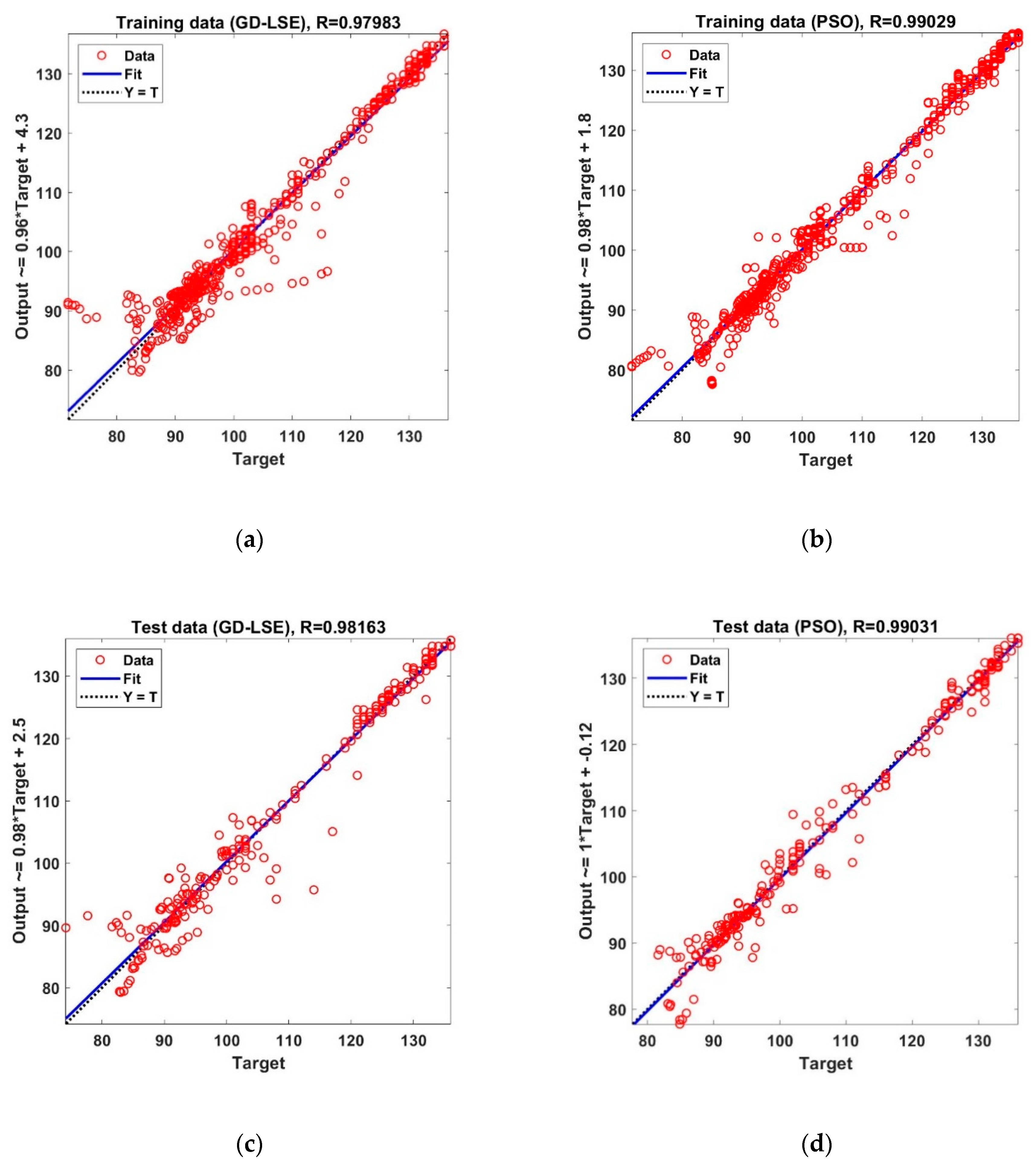
Furthermore, regression plots are shown in Figure 6, to illustrate the deviation of the predicted evaporator outlet temperatures from the experimentally obtained evaporator outlet temperatures. The linear correlation coefficient (R) for both GD-LSE and PSO models are listed in

Table 5. Summary of R coefficients obtained for the evaporator outlet temperature sub-model.

Training Method	Training Data	Test Data
GD-LSE	0.98	0.98
PSO	0.99	0.99

. Comparison of the R values indicate an acceptable fit for training and test data for both models. However, the R coefficients in the PSO model are closer to one, which imply better fit and greater generalisation ability of the model optimised by the PSO method. For the training and test datasets, the R coefficients improved 1.1% and 0.9%, respectively, by deploying the PSO method for training.

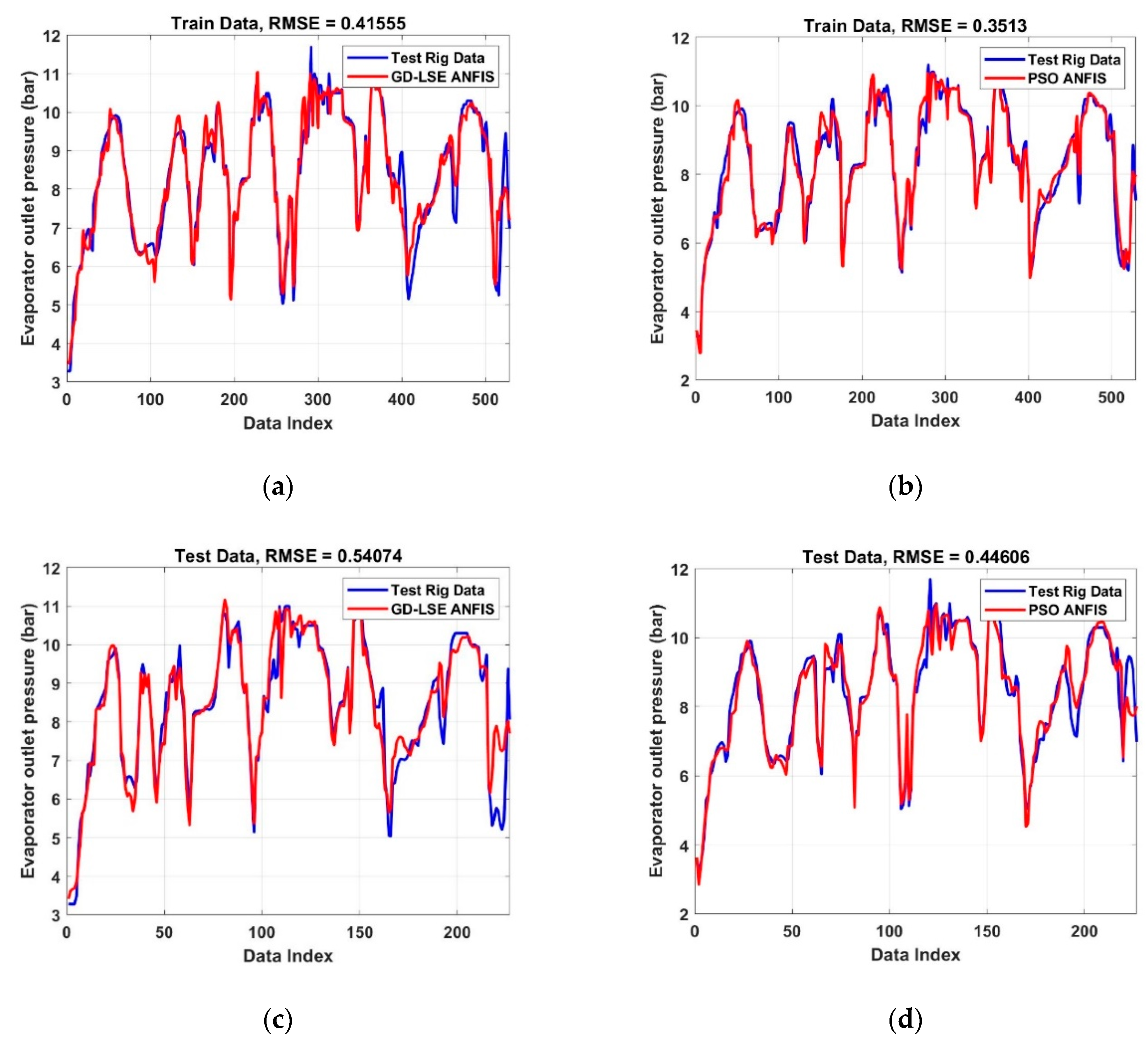
ANFIS model is applied to predict evaporator outlet pressure. The new sub-model is trained by deploying the GD-LSE technique and PSO technique. Comparison of the obtained RMSE values from both training and test dataset is presented in Figure 7. For the training dataset RMSE of 0.42 and 0.35 are achieved from the models trained using GD-LSE technique and PSO technique, respectively. The obtained RMSE for the unseen test data is 0.45 for the PSO ANFIS model and 0.54 for the GD-LSE model. It can be inferred that the evaporator outlet pressure results achieved from the PSO ANFIS model have a better compliance with the experimental data as evaluated against the model trained by the GD-LSE technique. For the training data, deploying the PSO algorithm to train the neuro fuzzy model results in 15% improvement in the RMSE as compared with the GD-LSE method. Moreover, for the test data the RMSE of the model trained using the PSO technique enhanced by 18%, which illustrates better generalisation ability in prediction of the evaporator outlet pressure.

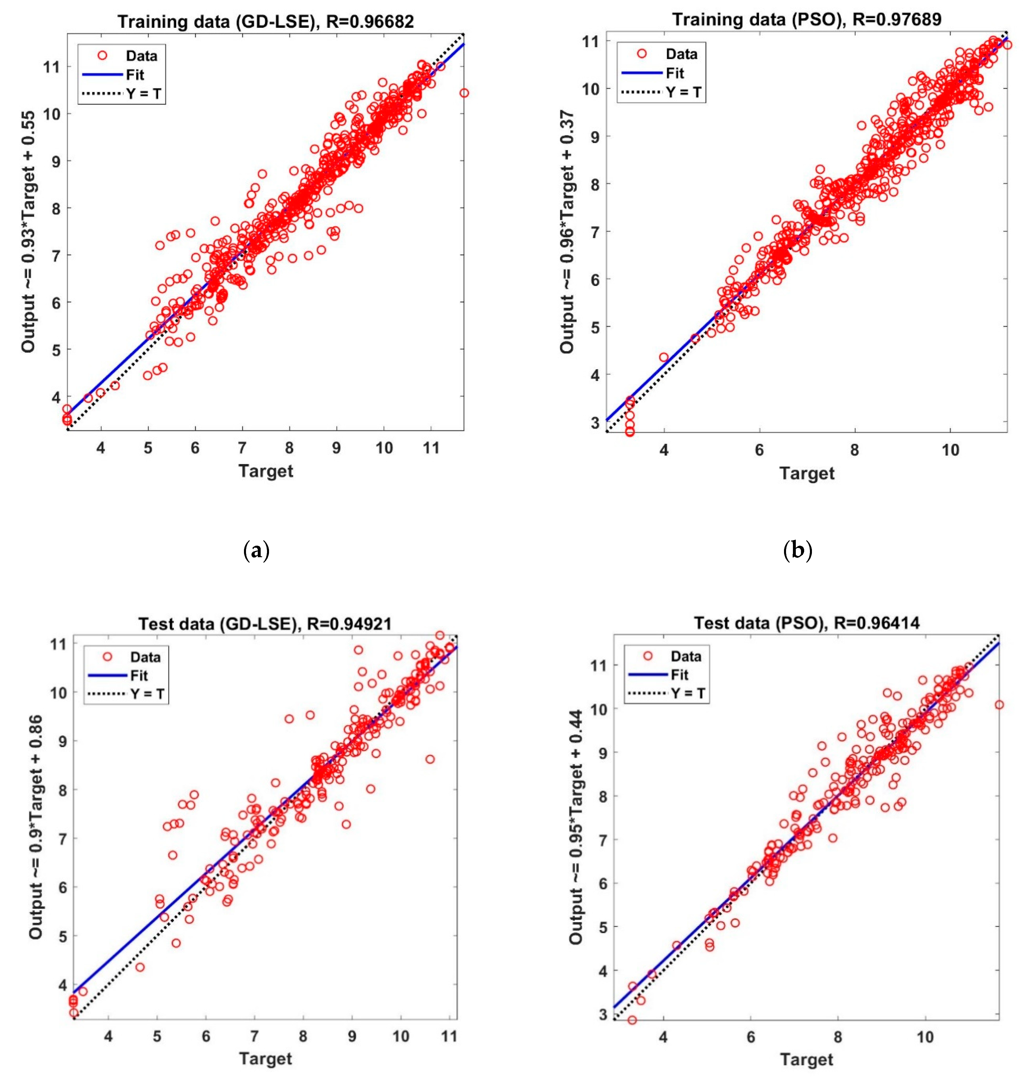
Similarly, to examine the accuracy of the models, comparison of the regression plots for the models trained by GD-LSE and PSO methods are shown in Figure 8. The R coefficient for the training and test data sets in both models are close to one, which indicates the agreement between the predictions from the models and the experimentally measured evaporator outlet pressures. The obtained linear correlation coefficients are listed in

Table 6. Summary of R coefficients obtained for the evaporator outlet pressure sub-model.

Training Method	Training Data	Test Data
GD-LSE	0.96	0.95
PSO	0.98	0.96

. The R values achieved for the training and test data sets are higher in the PSO model. Furthermore, the highest obtained accuracy is for the refrigerant output pressure model optimised using PSO algorithm with the linear correlation coefficient of 0.98 for the training dataset, and 0.96 for the test dataset. These two sub-models for the evaporator outlet temperature and evaporator outlet pressure can be used to identify the phase of the working medium instantaneously. Therefore, in the application of the ORC for recovery of the wasted heat in IC engines, this neuro-fuzzy model can be deployed to design an accurate control system to ensure the system safety and prevent decomposition of the working fluid by adjusting the pump speed.

The neuro-fuzzy models developed to predict the evaporator outlet temperature and evaporator outlet pressure are very agile due to the modelling benefits of fuzzy systems. Compared to the conventional models of evaporator such as FV and MB models, the neuro-fuzzy models do not require numerical solution of governing differential equations, and therefore, are computationally less expensive. The accuracy and speed of the neuro-fuzzy evaporator models illustrate its potential for real-time control purposes.

7. Conclusions

In this study, GD-LSE and PSO algorithms have been to train two neuro-fuzzy models for prediction of the evaporator outlet temperature and pressure of a 1-kWe ORC prototype. As system safety is vital in ORC applications for the recovery of waste heat from the exhaust gases of IC engines, accurate modelling of the evaporator outlet temperature, and pressure plays a pivotal role in the design of suitable control systems. Comparisons of experimentally gathered data and predictions from the neuro-fuzzy models reveal an acceptable accuracy in predicting the evaporator outlet temperature and pressure.

Based on the obtained results the main findings from this study are as follows:

• The neuro-fuzzy models offer reduced complexity, high accuracy and lower computational burden for prediction of the evaporator outlet temperature and pressure.
• The models developed by using neuro-fuzzy technique can be deployed for real-time control of ORC in various applications.
• Compared to the models trained using the GD-LSE algorithm, the models trained using the population-based PSO algorithm obtained better accuracy in terms of RMSEs and R coefficients for the training and test datasets. For the evaporator outlet temperature, a 29% improvement in the RMSE was achieved for both the training and test data. Furthermore, the evaporator outlet pressure RMSE improved by 15% and 18% for the training and test data, respectively, by using the PSO algorithm.
• The effort to identify the model parameters reduced substantially in the ANFIS models as opposed to the conventional non-adaptive methods of fuzzy system tuning.

References

1. Saliba, G.; Saleh, R.; Zhao, Y.; Presto, A.A.; Lambe, A.T.; Frodin, B.; Sardar, S.; Maldonado, H.; Maddox, C.; May, A.A.; et al. Comparison of gasoline direct-injection (GDI) and port fuel injection (PFI) vehicle emissions: Emission certification standards, cold-start, secondary organic aerosol formation potential, and potential climate impacts. Environ. Sci. Technol. 2017, 51, 6542–6552. [Google Scholar] [CrossRef]
2. Lecointe, B.; Monnier, G. Downsizing a gasoline engine using turbocharging with direct injection. SAE Tech. Paper Ser. 2003, 1, 542. [Google Scholar] [CrossRef]
3. Ciatti, S.; Johnson, M.; Das Adhikary, B.; Reitz, R.D.; Knock, A. Efficiency and emissions performance of multizone stratified compression ignition using different octane fuels. SAE Tech. Paper Ser. 2013, 1, 263. [Google Scholar] [CrossRef]
4. Armstead, J.R.; Miers, S.A. Review of waste heat recovery mechanisms for internal combustion engines. J. Therm. Sci. Eng. Appl. 2013, 6, 014001. [Google Scholar] [CrossRef]
5. Sprouse, C.; Depcik, C. Review of organic Rankine cycles for internal combustion engine exhaust waste heat recovery. Appl. Therm. Eng. 2013, 51, 711–722. [Google Scholar] [CrossRef]
6. Yang, K.; Zhang, H.; Song, S.; Zhang, J.; Wu, Y.; Zhang, Y.; Wang, H.; Chang, Y.; Bei, C. Performance analysis of the vehicle diesel engine-ORC combined system based on a screw expander. Energies 2014, 7, 3400–3419. [Google Scholar] [CrossRef] [Green Version]
7. Katsanos, C.; Hountalas, D.; Pariotis, E. Thermodynamic analysis of a Rankine cycle applied on a diesel truck engine using steam and organic medium. Energy Convers. Manag. 2012, 60, 68–76. [Google Scholar] [CrossRef]
8. Freymann, -I.H.R.; Strobl, D.-I.W.; Obieglo, S.T.A. The turbosteamer: A system introducing the principle of cogeneration in automotive applications. MTZ Worldw. 2008, 69, 20–27. [Google Scholar] [CrossRef]
9. Enayatollahi, H.; Fussey, P.; Nguyen, B. Control of organic Rankine cycle, a neuro-fuzzy approach. Control. Eng. Pract. 2021, 109, 104728. [Google Scholar] [CrossRef]
10. Yu, G.; Shu, G.; Tian, H.; Wei, H.; Liu, L. Simulation and thermodynamic analysis of a bottoming organic Rankine cycle (ORC) of diesel engine (DE). Energy 2013, 51, 281–290. [Google Scholar] [CrossRef]
11. Dai, Y.; Wang, J.; Gao, L. Parametric optimization and comparative study of organic Rankine cycle (ORC) for low grade waste heat recovery. Energy Convers. Manag. 2009, 50, 576–582. [Google Scholar] [CrossRef]
12. Le Brun, N.; Simpson, M.; Acha, S.; Shah, N.; Markides, C.N. Techno-economic potential of low-temperature, jacket-water heat recovery from stationary internal combustion engines with organic Rankine cycles: A cross-sector food-retail study. Appl. Energy 2020, 274, 115260. [Google Scholar] [CrossRef]
13. Simpson, M.C.; Chatzopoulou, M.A.; Oyewunmi, O.A.; Le Brun, N.; Sapin, P.; Markides, C.N. Technoeconomic analysis of internal combustion engine–organic Rankine cycle systems for combined heat and power in energy-intensive buildings. Appl. Energy 2019, 253, 113462. [Google Scholar] [CrossRef]
14. Wang, E.; Zhang, H.; Fan, B.; Ouyang, M.; Zhao, Y.; Mu, Q. Study of working fluid selection of organic Rankine cycle (ORC) for engine waste heat recovery. Energy 2011, 36, 3406–3418. [Google Scholar] [CrossRef]
15. van Kleef, L.M.; Oyewunmi, O.; Markides, C.N. Multi-objective thermo-economic optimization of organic Rankine cycle (ORC) power systems in waste-heat recovery applications using computer-aided molecular design techniques. Appl. Energy 2019, 251, 112513. [Google Scholar] [CrossRef]
16. Oyewunmi, O.; Taleb, A.I.; Haslam, A.J.; Markides, C.N. On the use of SAFT-VR Mie for assessing large-glide fluorocarbon working-fluid mixtures in organic Rankine cycles. Appl. Energy 2016, 163, 263–282. [Google Scholar] [CrossRef] [Green Version]
17. White, M.; Oyewunmi, O.; Chatzopoulou, M.; Pantaleo, A.; Haslam, A.; Markides, C. Computer-aided working-fluid design, thermodynamic optimisation and thermoeconomic assessment of ORC systems for waste-heat recovery. Energy 2018, 161, 1181–1198. [Google Scholar] [CrossRef]
18. Chatzopoulou, M.A.; Lecompte, S.; De Paepe, M.; Markides, C.N. Off-design optimisation of organic Rankine cycle (ORC) engines with different heat exchangers and volumetric expanders in waste heat recovery applications. Appl. Energy 2019, 253, 113442. [Google Scholar] [CrossRef]
19. Schuster, S.; Markides, C.N.; White, A.J. Design and off-design optimisation of an organic Rankine cycle (ORC) system with an integrated radial turbine model. Appl. Therm. Eng. 2020, 174, 115192. [Google Scholar] [CrossRef]
20. Van Erdeweghe, S.; Van Bael, J.; Laenen, B.; D’Haeseleer, W. Design and off-design optimization procedure for low-temperature geothermal organic Rankine cycles. Appl. Energy 2019, 242, 716–731. [Google Scholar] [CrossRef]
21. Chatzopoulou, M.A.; Simpson, M.; Sapin, P.; Markides, C.N. Off-design optimisation of organic Rankine cycle (ORC) engines with piston expanders for medium-scale combined heat and power applications. Appl. Energy 2019, 238, 1211–1236. [Google Scholar] [CrossRef]
22. Freeman, J.; Hellgardt, K.; Markides, C.N. An assessment of solar-powered organic Rankine cycle systems for combined heating and power in UK domestic applications. Appl. Energy 2015, 138, 605–620. [Google Scholar] [CrossRef] [Green Version]
23. Wei, D.; Lu, X.; Lu, Z.; Gu, J. Dynamic modeling and simulation of an Organic Rankine Cycle (ORC) system for waste heat recovery. Appl. Therm. Eng. 2008, 28, 1216–1224. [Google Scholar] [CrossRef]
24. Chowdhury, J.I.; Nguyen, B.K.; Thornhill, D. Modelling of evaporator in waste heat recovery system using finite volume method and fuzzy technique. Energies 2015, 8, 14078–14097. [Google Scholar] [CrossRef] [Green Version]
25. Horst, T.A.; Rottengruber, H.-S.; Seifert, M.; Ringler, J. Dynamic heat exchanger model for performance prediction and control system design of automotive waste heat recovery systems. Appl. Energy 2013, 105, 293–303. [Google Scholar] [CrossRef]
26. Desideri, A.; Dechesne, B.; Wronski, J.; Broek, M.V.D.; Gusev, S.; Lemort, V.; Quoilin, S. Comparison of moving boundary and finite-volume heat exchanger models in the Modelica language. Energies 2016, 9, 339. [Google Scholar] [CrossRef] [Green Version]
27. Enayatollahi, H.; Fussey, P.; Nguyen, B.K. Modelling evaporator in organic Rankine cycle using hybrid GD-LSE ANFIS and PSO ANFIS techniques. Therm. Sci. Eng. Prog. 2020, 19, 100570. [Google Scholar] [CrossRef]
28. Chowdhury, J.I.; Nguyen, B.K.; Thornhill, D.; Hu, Y.; Soulatiantork, P.; Balta-Ozkan, N.; Varga, L. Fuzzy nonlinear dynamic evaporator model in supercritical organic Rankine cycle waste heat recovery systems. Energies 2018, 11, 901. [Google Scholar] [CrossRef] [Green Version]
29. Jang, J.-S. ANFIS: Adaptive-network-based fuzzy inference system. IEEE Trans. Syst. Man Cybern. 1993, 23, 665–685. [Google Scholar] [CrossRef]
30. Khosravi, A.; Syri, S.; Zhao, X.; Assad, M.E.H. An artificial intelligence approach for thermodynamic modeling of geothermal based-organic Rankine cycle equipped with solar system. Geothermics 2019, 80, 138–154. [Google Scholar] [CrossRef]
31. Enayatollahi, H.; Fussey, P.; Nguyen, B.K. A neuro-fuzzy model of evaporator in organic Rankine cycle. In Proceedings of the 5th World Congress on Mechanical, Chemical, and Material Engineering 2019, Lisbon, Portugal, 15–17 August 2019. [Google Scholar]
32. Unamba, C.K.; Sapin, P.; Li, X.; Song, J.; Wang, K.; Shu, G.; Tian, H.; Markides, C.N. Operational optimisation of a non-recuperative 1-kWe organic Rankine cycle engine prototype. Appl. Sci. 2019, 9, 3024. [Google Scholar] [CrossRef] [Green Version]
33. Kharb, R.K.; Shimi, S.; Chatterji, S.; Ansari, F. modeling of solar PV module and maximum power point tracking using ANFIS. Renew. Sustain. Energy Rev. 2014, 33, 602–612. [Google Scholar] [CrossRef]
34. Esen, H.; Inalli, M.; Sengur, A.; Esen, M. Predicting performance of a ground-source heat pump system using fuzzy weighted pre-processing-based ANFIS. Build. Environ. 2008, 43, 2178–2187. [Google Scholar] [CrossRef]
35. Awadallah, M.A.; Bayoumi, E.H.; Soliman, H.M. Adaptive deadbeat controllers for brushless DC drives using PSO and ANFIS techniques. J. Electr. Eng. 2009, 60, 3–11. [Google Scholar]
36. Shoorehdeli, M.A.; Teshnehlab, M.; Sedigh, A.K.; Khanesar, M.A. Identification using ANFIS with intelligent hybrid stable learning algorithm approaches and stability analysis of training methods. Appl. Soft Comput. 2009, 9, 833–850. [Google Scholar] [CrossRef]
37. Shoorehdeli, M.A.; Teshnehlab, M.; Sedigh, A.K. Training ANFIS as an identifier with intelligent hybrid stable learning algorithm based on particle swarm optimization and extended Kalman filter. Fuzzy Sets Syst. 2009, 160, 922–948. [Google Scholar] [CrossRef]
38. Sargolzaei, A.; Faez, K.; Sargolzaei, S. A new method for Foetal Electrocardiogram extraction using Adaptive Nero-Fuzzy Interference System trained with PSO algorithm. In Proceedings of the 2011 IEEE International Conference on Electro/Information Technology, Mankato, MN, USA, 15–17 May 2011; pp. 1–5. [Google Scholar]
39. Turki, M.; Bouzaida, S.; Sakly, A.; M’Sahli, F. Adaptive control of nonlinear system using neuro-fuzzy learning by PSO algorithm. In Proceedings of the 2012 16th IEEE Mediterranean Electrotechnical Conference, Institute of Electrical and Electronics Engineers (IEEE), Hammamet, Tunisia, 25–28 March 2012; pp. 519–523. [Google Scholar]
40. Rini, D.P.; Shamsuddin, S.M.; Yuhaniz, S.S. Balanced the trade-offs problem of anfis using particle swarm optimization. TELKOMNIKA Telecommun. Comput. Electron. Control 2013, 11, 611–616. [Google Scholar] [CrossRef] [Green Version]
41. Karaboga, D.; Kaya, E. Training ANFIS using artificial bee colony algorithm. In 2013 IEEE INISTA; Institute of Electrical and Electronics Engineers (IEEE): New York, NY, USA, 2013; pp. 1–5. [Google Scholar]
42. Soto, J.; Melin, P.; Castillo, O. Optimization of interval type-2 fuzzy integrators in ensembles of ANFIS models for prediction of the Mackey-Glass time series. In Proceedings of the 2014 IEEE Conference on Norbert Wiener in the 21st Century (21CW), Boston, MA, USA, 24–26 June 2014; pp. 1–8. [Google Scholar]
43. Cárdenas, J.J.; García, A.; Romeral, J.L.; Kampouropoulos, K. Evolutive ANFIS training for energy load profile forecast for an IEMS in an automated factory. ETFA2011 2011, 1–8. [Google Scholar] [CrossRef]
44. Kennedy, J.; Eberhart, R. Particle swarm optimization. In Proceedings of the ICNN’95 International Conference on Neural Networks, Perth, Australia, 27 November–1 December 1995; Volume 4, pp. 1942–1948. [Google Scholar]
45. Kennedy, J. Swarm intelligence. In Handbook of Nature-Inspired and Innovative Computing; Springer: New York, NY, USA, 2006; pp. 187–219. [Google Scholar]
46. Kennedy, J. The behavior of particles. In International Conference on Evolutionary Programming; Springer: Berlin/Heidelberg, Germany, 1998; pp. 579–589. [Google Scholar]
Figure 1. Discretisation of evaporator into N control volumes [27].
Electronics 10 01535 g001
Figure 2. Piping and instrumentation diagram of ORC (organic Rankine cycle) testing facility (taken from [32]).
Electronics 10 01535 g002
Figure 3. Experimental test facility and ORC prototype (taken from [19]).
Electronics 10 01535 g003
Figure 4. Architecture of adaptive neuro-fuzzy inference system (ANFIS) used to model the evaporator.
Electronics 10 01535 g004
Figure 5. Comparison of GD-LSE ANFIS and PSO ANFIS model predictions of the evaporator outlet temperature, T r , out , using training and test data: (a) training data (GD-LSE); (b) training data (PSO); (c) test data (GD-LSE); and (d) test data (PSO).
Electronics 10 01535 g005
Figure 6. Comparison of regression plots between GD-LSE ANFIS and PSO ANFIS models for prediction of evaporator outlet temperature, T r , out , using the training and test data: (a) training data (GD-LSE); (b) training data (PSO); (c) test data (GD-LSE); and (d) test data (PSO).
Electronics 10 01535 g006
Figure 7. Comparison of GD-LSE ANFIS and PSO ANFIS model predictions of the evaporator outlet pressure, P r , out , using training and test data: (a) training data (GD-LSE); (b) training data (PSO); (c) test data (GD-LSE); and (d) test data (PSO).
Electronics 10 01535 g007
Figure 8. Comparison of regression plots between GD-LSE ANFIS and PSO ANFIS model predictions of the evaporator outlet pressure, P r , out , using training and test data: (a) training data (GD-LSE); (b) training data (PSO); (c) test data (GD-LSE); and (d) test data (PSO).
Electronics 10 01535 g008