Abstract
In analog circuit, the component parameters have tolerances and the fault component parameters present a wide distribution, which brings obstacle to classification diagnosis. To tackle this problem, this article proposes a soft fault diagnosis method combining the improved barnacles mating optimizer(BMO) algorithm with the support vector machine (SVM) classifier, which can achieve the minimum redundancy and maximum relevance for feature dimension reduction with fuzzy mutual information. To be concrete, first, the improved barnacles mating optimizer algorithm is used to optimize the parameters for learning and classification. We adopt six test functions that are on three data sets from the University of California, Irvine (UCI) machine learning repository to test the performance of SVM classifier with five different optimization algorithms. The results show that the SVM classifier combined with the improved barnacles mating optimizer algorithm is characterized with high accuracy in classification. Second, fuzzy mutual information, enhanced minimum redundancy, and maximum relevance principle are applied to reduce the dimension of the feature vector. Finally, a circuit experiment is carried out to verify that the proposed method can achieve fault classification effectively when the fault parameters are both fixed and distributed. The accuracy of the proposed fault diagnosis method is 92.9% when the fault parameters are distributed, which is 1.8% higher than other classifiers on average. When the fault parameters are fixed, the accuracy rate is 99.07%, which is 0.7% higher than other classifiers on average.
1. Introduction
Electronic devices often suffer from working continuously for a long time. With the increase of working time, the parameters of components may change, resulting in circuit performance degradation, or even severe damage to electronic devices. According to statistics, 80% of the faults occur mainly in analog circuits, which take account for 20% of the electronic devices [1]. Therefore, fault diagnosis methods for analog circuits have been a hotspot. Due to the complexity of analog circuits, fault diagnosis with high accuracy is challenging. The main reasons include: (1) the fault characteristics of analog circuits are very complex. It is difficult to find a feature extraction method suitable for all circuit faults with different circuit structures and different failure modes. (2) The input and output of analog circuits are mostly non-linear. The models of circuit components are also non-linear, which poses a significant challenge to the injection of test signals and the extraction of fault features. (3) Components in analog circuits have tolerance characteristics. When a fault occurs, the parameters of the faulty components present a wide distribution. This distribution may cause the coupling of the faulty features with the normal circuit characteristics, which makes it difficult to achieve classification diagnosis.
Fault diagnosis of analog circuits can be viewed as a multi-class problem. It consists of an efficient and accurate classifier, a component to excite and collect fault data, and feature vector extraction and selection.
For circuit fault diagnosis, the error sources that affect the diagnosis accuracy mainly include: (1) The performance difference of classifiers will affect the diagnosis accuracy; (2) The method of feature vector extraction, especially considering the tolerance and large range of fault distribution, will affect the accuracy of diagnosis.
First of all, an efficient and accurate classifier is the core part of fault classification. Support vector machine (SVM) [2,3], based on statistical learning theory, has the advantages of simple structure, clear theoretical explanation, and small training sample size. SVM is a supervised learning algorithms for binary and multivariate classification by searching for separating hyperplanes in the feature space. It can also deal with non-linear classification problems by introducing kernel functions. SVM is widely used in classification problems.
The selection of the penalty parameter and kernel function parameter of SVM significantly affects the classification accuracy [2]. Cross-grid validation is commonly used in the optimization of these parameters. Linear gridding establishes a grid within the optimization range to find each node. The optimization time and result are affected by grid resolution and vector space. The efficiency of the optimization is very low, resulting in a very long training time. Using various optimization algorithms developed by researchers combined with SVM can greatly improve the efficiency of optimization, such as genetic algorithm (GA) [4], particle swarm optimization (PSO) [5], ant lion optimization algorithm (ALO) [6] et al. Wolpert and Macready proposed the “No Free Lunch” theorems (NFL) [7], which proved that there is no best metaheuristic algorithm to solve all optimization problems, thus encouraging researchers to keep coming up with new optimization algorithms.
The barnacles matching optimizer (BMO) proposed by Sulaiman et al. [8] is a new biological population metaheuristic intelligent algorithm. It has the advantages of few adjustment parameters, fast convergence speed, and high accuracy. It has attracted researchers’ attention as soon as it is proposed and has been successfully applied to power system problems and economic dispatch problems. The convergence speed of BMO is very fast, however, it is easy to fall into the local optimum. How to use the optimization algorithm to build an efficient and accurate classifier is a problem worthy of study.
Second, feature extraction strategy for soft fault diagnosis of analog circuits directly affects the classification accuracy. When the parameters of fault elements change in an extensive range, especially when the tolerance of all components is considered, there may be a high correlation between the fault features and the fault-free features and between different fault features, which makes the classification difficult. At the same time, in order to make the data as complete as possible, the dimension of the feature vectors produced by general simulation is relatively high, which will produce a large amount of data. It is also a problem worth studying how to make effective fault excitation and feature vectors extraction and selection.
In order to solve the above two problems, this paper has made the following work: (1) an improved barnacle mating optimizer (IBMO) is proposed, which further enhances the convergence speed, exploration ability, and the ability to jump out of the local optimum of the IBMO. The performance is tested with six test functions. (2) The SVM classifier based on IBMO is designed and its performance is verified on three UCI datasets. (3) An analog circuit fault diagnosis method is designed. In order to solve the problem of analog circuit component parameter tolerance and fault parameter wide range distribution diagnosis, fuzzy set theory [9] combined with minimum redundancy maximum relevance (mRMR) [10] is proposed for feature selection. (4) The modeling and fault simulation is carried out for a circuit example. The fault diagnosis method is tested with the fault parameters both fixed and distributed. At the same time, the fuzzy parameters are discussed and the test results are analyzed.
This paper is presented as follows: Section 1 introduces the background, current problems, and the work of this paper. Section 2 introduces the classification theory of the support vector machine. In Section 3, the improved method of BMO is proposed, tested, and analyzed. In Section 4, the workflow of SVM based on the IBMO algorithm is introduced. Moreover, the test results on UCI data sets are provided. Section 5 introduces analog circuit fault diagnosis methods including fault data generation based on the simulator, feature selection based on fuzzy method, training and classification methods. In Section 6, the method described in this paper is tested on a circuit to verify the effectiveness. Section 7 summarizes the whole paper.
2. Review of Support Vector Machine Theory
The basic model of SVM is a linear binary classifier defined in the feature space. Nonlinear classification can be achieved by introducing kernel function and maximizing soft-margin. Defining the data sets , , and the hyperplane . The distance from the sample in S to the hyperplane is ,
The objective function of the distance maximization problem is as follows: Since some sample points in margin cannot satisfy the strong constraint conditions, the slack variable and penalty parameter c are introduced. The margin maximization problem can be transformed into a convex quadratic programming problem [2,11,12]:
When the problem is extended to nonlinear, the hyperplane is expressed as: . In this case, the quadratic programming problem is:
The Lagrange multiplier method is used to solve the dual problem. The Lagrange function is [13]:
where are Lagrange multipliers. The dual problem is transformed into:
After solving and , the hyperplane equation can be obtained as follows:
is the kernel function. The introduction of kernel function can save many calculations caused by the increase of dimension after mapping low dimensional space to high dimensional space in inner product operation. In this paper, the Gaussian kernel function is used.
It can be seen from the introduction above that the value of penalty parameter c and the Gaussian kernel function parameter γ have a significant influence on the SVM model and then affect the effect of SVM classification. Therefore, it is of great significance to find a suitable c and γ matching method to improve the classification accuracy. The optimization algorithm can improve the efficiency of SVM to find the optimal parameters.
3. The BMO Algorithm and the Improved Method
3.1. The BMO Algorithm
BMO algorithm is an evolutionary algorithm, which imitates the barnacle population in nature to produce new offspring, continuously iteratively improves the characteristics of the offspring, so as to obtain the global optimal solution. Barnacles have a robust reproductive capacity, and most barnacles are hermaphroditic, which means that they have heterosexual reproduction and self-reproduction [8].
BMO algorithm uses Hardy–Weinberg principle [8] to generate offspring. The frequency of Dad(D) and Mum(M) is expressed as f(D) = p and f(M) = q, respectively. For homozygotes, the expected genotype frequency under normal mating can be expressed as f(DD) = p2, f(MM) = q2, respectively. For heterozygotes, it is expressed as f(DM) = 2pq, and p2 + 2pq + q2 = 1 [14].
The population vector of BMO is expressed as:
where N is the number of variables and n is the number of populations.
The upper and lower bounds of variables can be expressed as:
The Equation (8) is used to sort the population of each generation randomly as the father group and mother group of the current generation [15].
The mating distance parameter is defined as pl. In the father group and mother group, only the parents less than or equal to parameter pl can reproduce and produce the next generation according to Equation (9):
where p is a random number between [0,1], q = 1 − p, p and q represent the proportion of fathers and mothers in their offspring.
When the distance between the parents in the father group and mother group exceeds the value of pl, the exploratory behavior occurs according to Equation (10).
All barnacles were sorted by fitness, and the optimal n individuals were selected. Through the continuous evolution of the population, the optimal performance is approached. Until the maximum number of iterations, the surviving population’s first barnacle is considered the global optimal value.
3.2. Improvement of the BMO Algorithm
- (1)
- Dynamic Search Scope Mechanism
In the BMO algorithm, the mating distance between the father group and mother group is affected by changing the value of parameter pl. The value of parameter pl has a significant influence on the convergence of the BMO algorithm. The value of parameter pl is discussed in the original algorithm. However, the fixed value will lead to premature convergence and insufficient exploitation capacity of the algorithm. Therefore, the introduction of the parameter pl dynamic random model makes pl change in a certain range, increasing the exploitation capacity of the algorithm. The model is expressed as follows:
where n is the number of populations.
- (2)
- Self-Reproduction Mechanism
In the BMO algorithm, heterozygous reproduction was simulated to simplify the model. Only the heterozygous frequency f(DM) = 2pq was introduced into the offspring gene. In the improved algorithm, the self-reproduction mechanism was added. According to Equation (12), individuals of each generation reproduce themselves to increase population specificity, which offers offspring superior performance.
where Y is the current position and Z is the offspring position.
- (3)
- Levy Flight Mechanism
In order to further enhance the exploitation ability and the ability to jump out of the local optimal solution, the concept of Levy flight [16] (LF) is introduced. LF is a kind of random walk, its direction of each step is completely random and isotropic, and the distribution of step size is heavy tailed. It has been proved that many biological trajectories, including many human behaviors, are based on LF, and the transfer behavior based on LF is optimal [17]. Therefore, the introduction of Levy flight into the algorithm can increase the diversity of the population, further increase the exploitation ability, and improve the ability of the algorithm to jump out of the local optimal solution. LF is performed for the last k individuals in each generation. The value of k is random, and its calculation method is shown in Equation (13). Equations (14) and (15) describe the mathematical model of LF, where Z represents the updated position, Y represents the current position, and S is the step size.
The pseudo code of the improved BMO algorithm is presented in IBMO Algorithm:
| IBMO Algorithm |
| Initial population number, position; The fitness value of each individual was calculated; The population was sorted in descending order according to fitness; while(Current iteration < Maximum iteration) The parameter k is calculated according to Equation (13): The k individuals at the end of the population were carried out Levy flight according to the Equations (14) and (15); The parameter pl is updated according to Equation (11); Mating and exploration activities were carried out according to the value range of parameter pl; Self-reproduction was performed according to Equation (12); The optimal new generation population was selected; end while Select the best individual. |
3.3. Test and Analysis
3.3.1. Test Functions
In order to thoroughly test the performance of the IBMO algorithm, six functions with different characteristics are used to evaluate the performance of the algorithm. F1 is the unimodal function, F2–F6 are the multimodal functions. For unimodal function, there is only one global optimal value in the definition domain, and there is no local extremum. It is used to test the exploration and the convergence ability. The multimodal function is easy to fall into local because it has multiple local optimal values. It can evaluate the exploitation ability, optimal global searchability, the ability to avoid premature convergence, and jump out of local optimal.
Table 1 shows the expressions and parameter settings of the six test functions. Figure 1 shows the graph of each test function of two dimension. In order to clearly show the detailed characteristics of the function, the definition domain of each function in the figure takes the local range, and the distribution characteristics of the optimal value of each test function can be found.

Table 1.
Test functions and parameters.
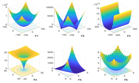
Figure 1.
Two-dimensional variable local graph of test function.
3.3.2. Test and Analysis
In order to test the performance of the IBMO, six test functions in Table 1 are applied on GA, PSO, ALO, BMO, and IBMO, respectively. Each algorithm runs 50 optimization calculations for six test functions. The best result, the worst result, and the average result of all test functions corresponding to each algorithm are calculated to evaluate the algorithm.
For the optimization algorithm, the maximum number of iterations and population can be adjusted according to the actual use. However, the larger numbers will lead to more computation, which will cost more resources and time. In order to compare the performance of several algorithms, the same parameters are selected for comparison.
The number of maximum iterations is 100 and the population is 30. As shown in Table 2, compared with the other four optimization algorithms, the best result, the worst result, and the average result of IBMO are better than other optimization algorithms in the test of six functions.
Table 2.
Test results of optimization algorithms.
Figure 2 shows the convergence curves of six test functions optimized by five algorithms. Figure 2a shows that in the unimodal function test, the optimization accuracy and convergence speed of IBMO are better than the other four algorithms. Moreover, in the multimodal function test, the IBMO algorithm finds the global expected minimum faster than other algorithms. Figure 2b shows that after the IBMO algorithm enters the local minimum value, it quickly jumps out of the local optimal value and continues to search for the global optimal value. Figure 2c,d shows that the IBMO algorithm converges to the desired accuracy faster than that of other algorithms. Figure 2e,f shows that the convergence speed and optimization accuracy of IBMO in complex multimodal function optimization is better than other algorithms. Combined with the data in Table 2, it can be seen that the best result, the worst result, and the average result of IBMO for unimodal function and multimodal function are better than that of other algorithms. It can be seen from Figure 2 and Table 2 that after the improvement of the original BMO algorithm in three aspects, the optimization accuracy, convergence speed, and the ability to jump out of the local minimum value of BMO algorithm are improved under the unimodal and multimodal functions tests.
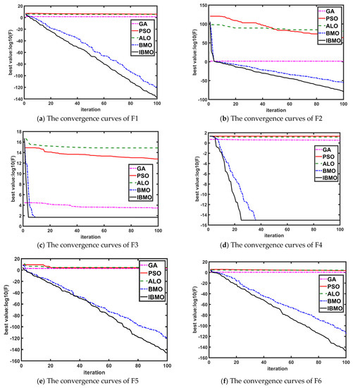
Figure 2.
Comparison of convergence curves of F1–F6 functions. (a–f) correspond to the convergence curves of F1 to F6 respectively.
4. SVM Classifier Based on IBMO
4.1. Optimization Process of SVM Parameters
In this paper, the IBMO algorithm is proposed to optimize the penalty parameter c in SVM and the kernel width parameter γ of the Gaussian kernel function. It is called the IBMO-SVM algorithm. The optimization process is presented as follows:
Step 1: Data initialization. According to the cross-validation parameters, the original data set is divided into the training set and the test set.
Step 2: IBMO initialization. Set the number of populations, the maximum number of iterations, variable dimension, and the search range.
Step 3: Fitness value calculation. The training set data are input into the SVM model, and the current generation c and γ are used to calculate the prediction accuracy of the test set data, which is used as the fitness value.
Step 4: Algorithm iteration. According to the fitness value, IBMO was used to update c and γ.
Step 5: Repeat steps 3 and 4 until the number of iterations is equal to the maximum number of iterations. At this time c and γ are the optimal parameters.
4.2. Testing Classifiers
In order to test the impact of the optimization algorithm on the performance of the classifier under the same number of iterations and population, the classifiers with five optimization algorithms are tested on UCI datasets [18]. As shown in Table 3, the datasets “iris,” “wine,” and “isolet5” are selected. The dataset “iris” is small in feature dimension, classification number, the total number of samples, and total data size, which can test the algorithm’s performance in small samples. The dataset “isolet5” has many classifications, feature dimensions, the total number of samples, and the total amount of data, which can test the algorithm’s performance when there are more classification and a large amount of data. The dataset “wine” is between the two datasets, moderate in all aspects. In order to reduce the randomness, each dataset was tested five times, and the average classification accuracy was taken.
Table 3.
The UCI test datasets.
The parameters set for each algorithm are shown in Table 4. The parameters Cr and Mi represent the crossover factor and the variant factor in the GA. The parameters c1 and c2 represent the weight of each particle’s best position and the weight of the neighborhood’s best position when adjusting velocity in the PSO. The parameter a represents the cross-validation parameter in SVM. In this paper, five-fold cross-validation was used. The dataset is divided into five parts, four of which are used as the training set and one as the test sets to calculate the classification accuracy when current parameters are used. In order to compare the performance of several algorithms, the same parameters need to be set. The population size, the maximum number of iterations, and the search range were taken to be 20, 50, and [0.001, 100].
Table 4.
Parameters of the algorithms.
As shown in Table 5, the SVM is optimized by using five algorithms. The classification accuracy of the three data sets is tested and compared. The results show that, due to the high efficiency of IBMO and the ability to jump out of the local optimal value, the classification accuracy of IBMO-SVM classifier is better than other classifiers in the case of classification number, feature dimension, total number of samples, and total amount of data with different characteristics.
Table 5.
Comparison of test accuracy results of classifiers.
5. The Analog Circuit Fault Diagnosis Method
The analog circuit fault diagnosis method designed in this paper is shown in Figure 3. It includes (1) fault simulation and data acquisition; (2) fault feature selection; (3) training and fault classification.
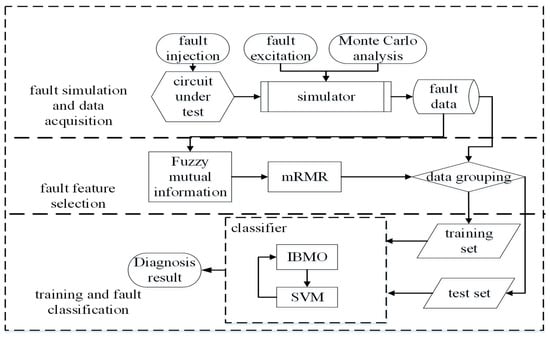
Figure 3.
Diagram of the analog circuit fault diagnosis method.
5.1. Fault Simulation and Data Acquisition
The circuit under test is modeled in the simulator. In order to approach the real situation, all components consider the tolerance and obey the Gaussian distribution as follows: V~N(ρ, (ρτ/3)2), where V is the real value of components, ρ is the nominal value of components, τ is the component tolerance.
In many research papers, the failure parameters of fault simulation components is defined as a fixed value or in a small range, such as literatures [1,19,20,21,22,23]. But in practice, all the components have tolerance, besides, when a component fails, the parameters may change over an extensive range. When various faults occur, this wide range of parameter changes will significantly aggravate the similarity of fault feature vectors, which will bring great difficulties to fault diagnosis.
Suppose that q1 and q2 are the minimum and maximum ratios when the parameter decreases, q3 and q4 are the minimum and maximum ratios when the parameter increases, the parameters of the faulty components follow the mean distribution. So the parameter distribution of the component in case of fault meets the requirements of WL ~ U(q1, q2)ρ or WH ~ U(q3, q4)ρ, where WL is the fault value when the component parameter decreases, and WH is the fault value when the component parameter increases. The distributions of other normal component parameters still follow Gaussian distribution.
The fault excitation is carried out in the simulator when all component parameters are normal, decreased, or increased. In the excitation of circuit soft fault, some scholars use the pulse excitation method. The circuit’s impulse response is sampled at high speed, and then the feature vectors are obtained by wavelet packet transform [24], S-transform [22], and Hilbert-Huang transform [25]. With these methods, the pulse excitation duration is very short, which requires steep pulse to reach a microsecond level and the rising and falling edges. The signal requires a high demand for the signal source. Simultaneously, the circuit pulse response needs to be sampled at high speed to obtain the circuit’s response curve during the excitation period. In this circumstance, the sampling rate must reach hundreds of megahertz or even thousands of megahertz, which puts forward a very high requirement for the circuit response signal extraction. It is challenging to achieve it in engineering.
This paper uses a method to extract the amplitude-frequency curve of output response by frequency conversion signal [26]. In this way, the requirement of the signal source is relatively low. Besides, after feature selection, only some individual frequency excitation signals are needed. The amplitude of the output waveform can be converted into a DC signal through the amplitude extraction circuit. With this method, only a low sampling rate is needed, and the requirement of sampling equipment is also low.
The amplitude-frequency response curve of the test point of each faulty circuit is obtained by frequency-scanning excitation. The amplitudes of K frequency points are collected for each curve as a sample. The feature dimension of each group of samples is K. Suppose that there are M components to be analyzed in the circuit. The fault-free condition is also regarded as a fault classification. There are (2M + 1) fault labels. N times Monte Carlo analysis and simulation for each fault class, all classes can get (2M + 1) × N groups of simulation samples.
5.2. Fault Feature Selection
The total sample space data, including all sample data and label data, is (2M + 1) × N × (K + 1). When the feature dimension K of the sample is large, a huge amount of data can be generated, which will consume a lot of resources and time in training, thus reducing the training efficiency. Because of the redundancy of feature vectors, feature dimensionality reduction can be achieved by feature selection.
5.2.1. Fuzzy Mutual Information in Sample Space
The mutual information of two discrete random variables S and T is defined as [27]:
where is the joint probability distribution function of S and T, and are the marginal probability distribution functions of S and T, respectively. At the same time, the mutual information can be expressed as [28]:
where H(S) and H(T) are the marginal entropy of S and T, respectively, and H(S, T) is the joint entropy of S and T.
I(S; T) = H(S) + H(Y) − H(S, T)
In this paper, fuzzy set theory is introduced to analyze the fuzzy relationship between feature vector and classification.
Define is the universe of discourse, where l is the number of elements in U. Assume p is a set of fuzzy attributes on U. It generates a fuzzy equivalent partition of c classes on U. The fuzzy equivalence matrix of attribute vector p corresponding to all classes is , where represents the membership of the j-th element of fuzzy attribute p to the i-th classification [29].
Suppose that the set of sample spaces corresponding to all classification of element attributes is . In this paper, the definition of membership function proposed by Khushaba [9] is selected. The membership of the k-th vector belonging to the i-th class is expressed as [9]:
where m is the fuzzification parameter, is a minimal positive number to avoid singularity, is the standard deviation involved in the distance computation. denotes the mean of the data sample that belong to class i, and is the radius of the data.
According to the Equation (17), the fuzzy mutual information between a feature vector f and the class vector C in the feature vector set , and the fuzzy mutual information between the two feature vectors fj and fk can be described as:
According to 5.1, there are a total of c = 2M + 1 class, and the class vector can be obtained. According to the sampling frequency K, the feature vector set can be obtained. According to the Monte Carlo simulation times N, the total number of samples of each feature vector is T = (2M + 1) × N.
The membership of feature vector f to all classes is calculated by Equation (18). A fuzzy relation matrix of feature vector f can be obtained as follows:. Similarly, the fuzzy relation matrices of two vector vectors and in feature vector set F are as follows: and . Denote the i-th row vector of as . The marginal fuzzy entropy of feature vector and the joint fuzzy entropy between two feature vectors are defined as follows [30]:
The occurrence frequency of each label is counted, and then the entropy of the classes is given as follows:
Calculate the probability of each label:, where represents the number of each label and T represents the number of samples. In this case, the entropy of the classes can be calculated as follows:
The joint fuzzy entropy of feature vector f and class vector C is given as follows [31]:
The fuzzy mutual information of feature vector f and class vector C, and the fuzzy mutual information between two feature vectors and can be obtained by introducing Equations (21)–(24) into Equations(19) and (20), respectively.
5.2.2. Dimension Reduction of Sample Space
The mRMR is a feature selection algorithm based on mutual information. It maximizes the mutual information between the selected features and the joint distribution of classification variables, and minimizes the mutual information between features, so as to obtain the optimal feature set. For the sample space and target set c with dimension N, the subspace feature set S is the optimal feature set. The maximum relevance principle is that the mean value of mutual information of all features in S and c is the largest:
In this case, the minimum redundancy principle is used to remove the redundant features in the subspace [32]:
Using the method of mutual information difference (MID) or mutual information quotient (MIQ), the optimal feature set satisfying mRMR principle is obtained as follows:
Set the number of the feature vectors (NOFV). Assume that all the sets are A, and the current set has been obtained. Use the incremental search method shown in Equations (29) or (30) to find the next feature vector in the remaining space until all the features meeting the number requirements are found.
In the incremental calculation process of the mRMR algorithm, the mutual information between feature vectors needs to be calculated in each iteration. Ahmed et al. improved the mRMR algorithm and proposed an enhanced minimum redundancy maximum relevance (EmRMR) method [10]. The mutual information between all feature vectors is stored and used in each iteration process by creating an empty order list. The index form is used to reduce unnecessarily repeated calculation in the iteration process. This method does not affect the results of mRMR selection. It reduces the redundant calculation process, and improves the algorithm efficiency.
This paper combines fuzzy mutual information and EmRMR method to achieve the feature selection of feature vectors, which is called Fuzzy Mutual Information-Enhanced Minimal Redundancy Maximal Relevance (FMI-EmRMR). The fuzzy mutual information between feature vectors and the fuzzy mutual information between feature vectors and class vector obtained by the method described in 5.2.1 are brought into Equation (29) or (30), and the sets of all and are brought into the iteration in the form of index, so as to obtain the feature vectors selected by FMI-EmRMR.
5.3. Training and Fault Classification
The FMI-EmRMR algorithm is adopted to select the feature vector, and the fault simulation data are divided into training set and test set. The training set is used to train IBMO-SVM, and the optimization process described in 4.1 is used to optimize the penalty parameter c and kernel function parameter γ of SVM. After training and optimization, the optimized parameters for classifier can be obtained. A classification test is carried out on test set. The classification accuracy is defined as a performance index of the algorithm.
6. Analog Circuit Fault Diagnosis Test
As shown in Figure 4, in multisim14.1, the Sallen-key band-pass filter circuit is modeled. The output node of the operational amplifier is used as the signal acquisition node. According to 5.1, ρ is the nominal value of resistance and capacitance, the tolerance of resistance and capacitance is set as τ = 5%, and the component parameter distribution is V ~ N(ρ, (0.0167ρ)2). When the component changes within its tolerance range, the circuit is fault-free. When the component deviates from the normal tolerance range, it is considered to have a soft fault. Suppose that the minimum detectable scale [29] of fault is 2τ = 0.1, so q2 = 1−2τ = 0.9, q3 = 1 + 2τ = 1.1. Let q1 = 0.1, q4 = 2, then the parameter distribution of faulty components satisfies WL ~ U(0.1, 0.9)ρ and WH ~ U(1.1, 2)ρ.
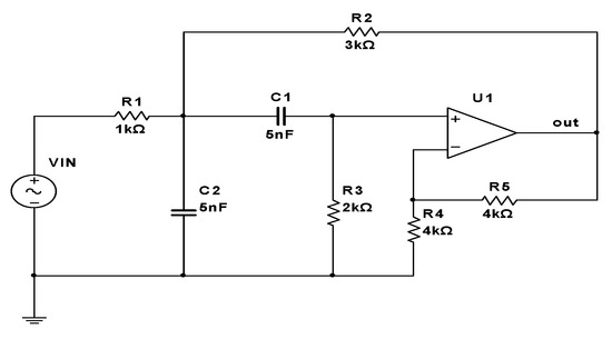
Figure 4.
Sallen-key circuit diagram.
As shown in Table 6, the values of the faulty components’ parameters in the range of variation and ±50% deviation from the fixed value are listed, respectively.
Table 6.
Fault description.
There are seven components in the circuit, so M = 7, then the number of class labels is (2M + 1) = 15. In the simulator, a sine wave with the peak value of 3V is used for linear frequency conversion scanning from 1 Hz to 300 kHz, and 1000 frequency sampling points are set at equal intervals, that is, the feature vector dimension K = 1000. The total number of samples is (2M + 1) × N =1500 by N = 100 Monte Carlo simulation analysis for each fault parameter circuit. The samples are divided into two groups evenly according to the classification, one as the training set and the other as the test set.
Figure 5a shows the amplitude-frequency response curves of 100 times Monte Carlo simulation for L1, L3, L7, L13, and L14 faults with fixed fault values. Figure 5b shows the amplitude–frequency response curves with the fault distribution uniform in an extensive range. When a fixed fault value is adopted, the amplitude–frequency response curve of each type of fault is relatively concentrated, and the curve characteristics between each type of fault are apparent, and the identification degree is high. When the fault value is distributed in an extensive range, the amplitude–frequency response curve of each type of fault is wildly divergent, and the curve features of each type of fault overlap more. The identification degree is low, which significantly improves the difficulty of diagnosis.
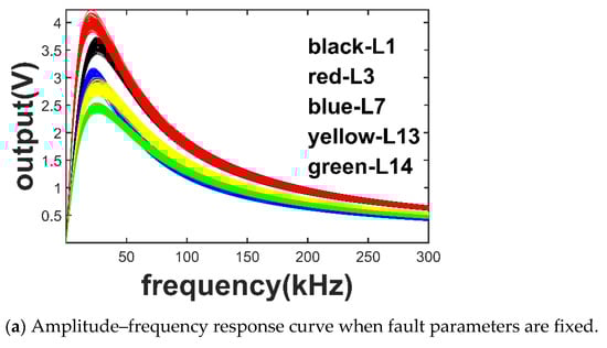
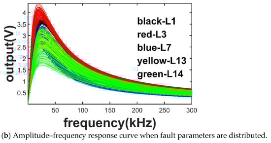
Figure 5.
Amplitude–frequency response curves of several labels of faults in two cases.
In order to reduce the dimension of features, the method of FMI-EmRMR is used to select feature vectors. By calculating the fuzzy mutual information between each frequency point vector and the fuzzy mutual information between each frequency point vector and the class vector in the sample space, as the input of EmRMR, the feature frequency points can be obtained.
Since the fuzzification parameter m in the membership function will affect the output of fuzzy mutual information, which may affect the output of EmRMR, the classification accuracy of different values of m is tested. It can be considered that when the number of selected dimensions in EmRMR is fixed, that is, when the feature vector is in the same feature dimension, the influence of m value on the accuracy of test classification can be characterized. As shown in Figure 6, different m values from 1.1 to 10 are tested. In this example, when the fault parameters are fixed, due to the strong independence between features, the influence of m on the accuracy is limited, and all values can ensure very high classification accuracy. When m is 4.3, the classification accuracy is the highest. When the fault parameters are distributed, the overlap between features is severe. At this time, the fuzzy parameters have a certain impact on the classification accuracy. When m is 3.9, the classification accuracy is the highest.
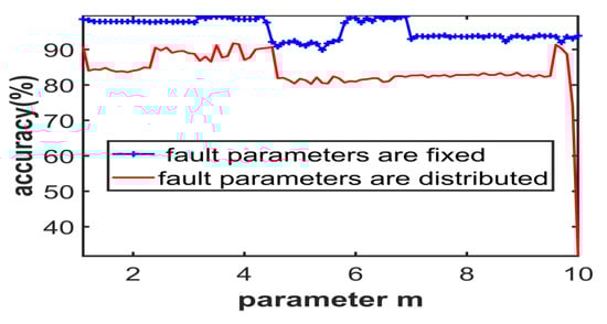
Figure 6.
The curve of the influence of parameter m on accuracy under two kinds of fault parameters.
As shown in Table 7, the search range of all classifiers is [0.001, 1000], the population size is 20, and the maximum number of iterations is 50. The fuzzification parameter m is set to 3.9 and 4.3, respectively. The feature frequency points are {20.421, 20.121, 19.820, 8.109, 2.103, 1.802, 1.502} kHz and {31.832, 31.532, 31.232, 23.124, 22.823, 21.622,21.322} kHz, respectively. Using the method described in this paper, very high classification accuracy can be obtained if the fixed fault values are used. However, when the fault parameters are evenly distributed in a large range, the diagnosis difficulty is much greater than that of the fixed fault values. The proposed method can still obtain higher accuracy to realize the classification of fault types. At the same time, the accuracy of the IBMO-SVM classifier is higher than other classifiers in both cases.
Table 7.
Comparison of fault diagnosis accuracy.
7. Conclusions
In this paper, an efficient method of the analog circuit fault diagnosis is presented. The main contributions of the proposed method includes: (1) The original BMO algorithm is improved. By using test functions to compare the optimization ability of several optimization algorithms, it shows that the improved BMO algorithm has higher optimization ability than the other algorithms and improves the optimization and convergence ability of the algorithm; (2) an improved BMO algorithm is proposed to optimize the SVM classifier, and the performance of the classifier is tested. Test data show that IBMO algorithm can effectively improve the efficiency of SVM parameters optimization and classification accuracy; (3) a feature selection algorithm based on fuzzy mutual information and enhanced mRMR is proposed. It can effectively extract the feature vector when the circuit components are in tolerance and the value of fault components is in a large fault range. The influence of the fuzzification parameter on fault diagnosis is analyzed, which improves the accuracy of fault diagnosis in a large fault range; (4) combined with the proposed classifier and feature method, a fault diagnosis method is designed. Considering the wide fault range of component parameters, the fault parameters are more consistent with the actual fault diagnosis. The characteristics of soft fault are simulated by signal injection, and the proposed diagnosis method is tested. The circuit test of an example shows that the method of IBMO-SVM classifier and FMI-EmRMR feature selection has high accuracy in the case of fixed fault values and distributed fault values. The accuracy of the proposed fault diagnosis method is 92.9% when the fault parameters are distributed, which is 1.8% higher than other classifiers on average. When the fault parameters are fixed, the accuracy rate is 99.07%, which is 0.7% higher than other classifiers on average.
The future work includes: (1) The influence of different membership function on the accuracy of classification and diagnosis; (2) how to further improve the convergence speed of the optimization algorithm; (3) the influence of other feature selection algorithms on fault diagnosis accuracy in an extensive fault range.
Author Contributions
Conceptualization, methodology, investigation, software, writing—original draft, H.L.; writing—review and editing, Y.Z.; resources, D.Z.; data curation, L.C.; validation, Y.L.; supervision, X.Z.; funding acquisition; project administration, Y.G. All authors have read and agreed to the published version of the manuscript.
Funding
This research was funded by National Natural Science Foundation of China, grant number 61973167.
Conflicts of Interest
The authors declare no conflict of interest. The funders had no role in the design of the study; in the collection, analyses, or interpretation of data; in the writing of the manuscript, or in the decision to publish the results.
References
- Zhang, C.; He, Y.; Yuan, L.; Xiang, S. Analog Circuit Incipient Fault Diagnosis Method Using DBN Based Features Extraction. IEEE Access 2018, 6, 23053–23064. [Google Scholar] [CrossRef]
- Du, J.; Liu, Y.; Yu, Y.; Yan, W. A Prediction of Precipitation Data Based on Support Vector Machine and Particle Swarm Optimization (pso-svm). Algorithms 2017, 10, 57. [Google Scholar] [CrossRef]
- Nguyen, L. Tutorial on Support Vector Machine. Special Issue “some Novel Algorithms for Global Optimization and Relevant Subjects”. Appl. Comput. Math. 2016, 6, 1–15. [Google Scholar]
- Khozani, S. Application of a Genetic Algorithm in Predicting the Percentage of Shear Force Carried By Walls in Smooth Rectangular Channels. Meas. J. Int. Meas. Confed. 2016, 87, 87–98. [Google Scholar] [CrossRef]
- Eberhart, R.; Kennedy, J. A New Optimizer Using Particle Swarm Theory. In Proceedings of the International Symposium on Micro Machine and Human Science, Nagoya, Japan, 4–6 October 1995; pp. 39–43. [Google Scholar]
- Mirjalili, S. The Ant Lion Optimizer. Adv. Eng. Softw. 2015, 83, 80–98. [Google Scholar] [CrossRef]
- Wolpert, D.H.; Macready, W.G. No Free Lunch Theorems for Optimization. IEEE Trans. Evol. Comput. 1997, 1, 67–82. [Google Scholar] [CrossRef] [Green Version]
- Sulaiman, M.H.; Mustaffa, Z.; Saari, M.M.; Daniyal, H. Barnacles Mating Optimizer: A New Bio-inspired Algorithm for Solving Engineering Optimization Problems. Eng. Appl. Artif. Intell. 2020, 87, 103330. [Google Scholar] [CrossRef]
- Khushaba, R.N.; Al-jumaily, A.; Al-ani, A. Novel Feature Extraction Method Based on Fuzzy Entropy and Wavelet Packet Transform for Myoelectric Control. In Proceedings of the 2007 International Symposium on Communications and Information Technologies, Sydney, NSW, Australia, 17–19 October 2007; pp. 352–357. [Google Scholar]
- Ahmed, Y.A.; Koçer, B.; Huda, S.; Ali, B.; Al-rimy, S.; Hassan, M.M. A System Call Refinement-based Enhanced Minimum Redundancy Maximum Relevance Method for Ransomware Early Detection. J. Netw. Comput. Appl. 2020, 167, 102753. [Google Scholar] [CrossRef]
- Kuang, F.; Xu, W.; Zhang, S. A Novel Hybrid kpca and svm with GA Model for Intrusion Detection. Appl. Soft Comput. J. 2014, 18, 178–184. [Google Scholar] [CrossRef]
- Eseye, A.T.; Zhang, J.; Zheng, D. Short-term Photovoltaic Solar Power Forecasting Using a Hybrid Wavelet-pso-svm Model Based on Scada and Meteorological Information. Renew. Energy 2018, 118, 357–367. [Google Scholar] [CrossRef]
- Soumaya, Z.; Drissi Taoufiq, B.; Benayad, N.; Yunus, K.; Abdelkrim, A. The Detection of Parkinson Disease Using the Genetic Algorithm and Svm Classifier. Appl. Acoust. 2021, 171, 107528. [Google Scholar] [CrossRef]
- Sulaiman, M.H.; Mustaffa, Z.; Saari, M.M.; Daniyal, H.; Musirin, I.; Daud, M.R. Barnacles Mating Optimizer: An Evolutionary Algorithm for Solving Optimization. In Proceedings of the 2018 IEEE International Conference on Automatic Control and Intelligent Systems, I2CACIS, Shah Alam, Malaysia, 20 October 2018; pp. 99–104. [Google Scholar]
- Sulaiman, M.H.; Mustaffa, Z.; Saari, M.M.; Daniyal, H.; Daud, M.R.; Razali, S.; Mohamed, A.I. Barnacles Mating Optimizer: A Bio-inspired Algorithm for Solving Optimization Problems. In Proceedings of the 2018 IEEE/ACIS 19th International Conference on Software Engineering, Artificial Intelligence, Networking and Parallel/distributed Computing, SNPD, Busan, Korea, 27–29 June 2018; pp. 265–270. [Google Scholar]
- Chegini, S.N.; Bagheri, A.; Najafi, F. Psoscalf: A New Hybrid Pso Based on Sine Cosine Algorithm and Levy Flight for Solving Optimization Problems. Appl. Soft Comput. J. 2018, 73, 697–726. [Google Scholar] [CrossRef]
- Viswanathan, G.M.; Afanasyev, V.; Buldyrev, S.V.; Havlin, S.; da Luz, M.G.E.; Raposo, E.P.; Stanley, H.E. Levy Flights in Random Searches. Phys. A Stat. Mech. Appl. 2000, 43, 1–12. [Google Scholar] [CrossRef]
- Dua, D.; Graff, C. UCI Machine Learning Repository. University of California, School of Information and Computer Science: Irvine, CA, USA. Available online: http://archive.ics.uci.edu/ml (accessed on 8 June 2021).
- Zhang, C.; He, Y.; Yuan, L.; Li, Z. Analog circuit fault diagnosis based on GMKL-SVM method. Chin. J. Sci. Instrum. 2016, 37, 1989–1995. [Google Scholar]
- Hengrong, M.; Lisheng, Y.; Dongme, L.; Yigang, H.; Lifen, Y.; Lixin, Z.; Peng, C.; Beilei, Z.; Shuai, R.; School of Electrical Engineering and Automation; et al. Analogue circuit fault diagnosis based on SVM optimized by IPSO. J. Electron. Meas. Instrum. 2017, 31, 1239–1246. [Google Scholar]
- Chen, P.; Yuan, L.; He, Y.; Luo, S. An improved SVM classifier based on double chains quantum genetic algorithm and its application in analogue circuit diagnosis. Neurocomputing 2016, 211, 202–211. [Google Scholar] [CrossRef]
- Tan, Y.; Sun, Y.; Yin, X. Analog Fault Diagnosis Using S-transform Preprocessor and a Qnn Classifier. Meas. J. Int. Meas. Confed. 2013, 46, 2174–2183. [Google Scholar] [CrossRef]
- Arabi, A.; Bourouba, N.; Belaout, A.; Belaout, A.; Ayad, M. An Accurate Classifier Based on Adaptive Neuro-fuzzy and Features Selection Techniques for Fault Classification in Analog Circuits. Integration 2019, 64, 50–59. [Google Scholar] [CrossRef]
- Long, Y.; Xiong, Y.; He, Y.; Zhang, Z. A New Switched Current Circuit Fault Diagnosis Approach Based on Pseudorandom Test and Preprocess By Using Entropy and Haar Wavelet Transform. Analog. Integr. Circuits Signal Process. 2017, 91, 445–461. [Google Scholar] [CrossRef]
- Tang, S.; Li, Z.; Chen, L. Fault Detection in Analog and Mixed-signal Circuits by Using Hilbert-huang Transform and Coherence Analysis. Microelectron. J. 2015, 46, 893–899. [Google Scholar] [CrossRef]
- Ming-Zhe, G.; Ai-Qiang, X.; Xiao-Feng, T.; Wei, Z. Analog circuit Diagnostic Method Based on Multi-kernel Learning Multiclass Relevance Vector Machine. Acta Autom. Sin. 2019, 45, 434–444. [Google Scholar]
- Tang, C.; Yang, X.; Lv, J.; He, Z. Zero-shot Learning by Mutual Information Estimation and Maximization. Knowl. Based Syst. 2020, 194, 105490. [Google Scholar] [CrossRef]
- Miura, A.; Tomoeda, A.; Nishinari, K. Formularization of Entropy and Anticipation of Metastable States Using Mutual Information in One-dimensional Traffic Flow. Phys. A Stat. Mech. Appl. 2020, 560, 125152. [Google Scholar] [CrossRef]
- Maji, P.; Pal, S.K. Fuzzy–rough Sets for Information Measures and Selection of Relevant Genes from Microarray Data. IEEE Trans. Syst. Man Cybern. Part B 2009, 40, 741–752. [Google Scholar] [CrossRef] [PubMed]
- Al-ani, A.; Khushaba, R.N. A Population Based Feature Subset Selection Algorithm Guided by Fuzzy Feature Dependency. In International Conference on Advanced Machine Learning Technologies and Applications; Springer: Berlin/Heidelberg, Germany, 2012; pp. 430–438. [Google Scholar]
- Khushaba, R.N.; Kodagoda, S.; Lal, S.; Dissanayake, G. Driver Drowsiness Classification Using Fuzzy Wavelet-packet-based Feature-extraction Algorithm. IEEE Trans. Biomed. Eng. 2011, 58, 121–131. [Google Scholar] [CrossRef] [Green Version]
- Lin, Y.; Hu, Q.; Liu, J.; Duan, J. Multi-label Feature Selection Based on Max-dependency and Min-redundancy. Neurocomputing 2015, 168, 92–103. [Google Scholar] [CrossRef]
Publisher’s Note: MDPI stays neutral with regard to jurisdictional claims in published maps and institutional affiliations. |
© 2021 by the authors. Licensee MDPI, Basel, Switzerland. This article is an open access article distributed under the terms and conditions of the Creative Commons Attribution (CC BY) license (https://creativecommons.org/licenses/by/4.0/).