Article

Gradual Wear Diagnosis of Outer-Race Rolling Bearing Faults through Artificial Intelligence Methods and Stray Flux Signals

by
Israel Zamudio-Ramirez
1,2,
Roque A. Osornio-Rios
1,
Jose A. Antonino-Daviu
2,*,
Jonathan Cureño-Osornio
1 and
Juan-Jose Saucedo-Dorantes
1
1
Engineering Faculty, San Juan del Río Campus, Universidad Autónoma de Querétaro, Av. Río Moctezuma 249, San Juan del Río, Querétaro 76807, Mexico
2
Instituto Tecnológico de la Energía, Universitat Politècnica de València (UPV), Camino de Vera s/n, 46022 Valencia, Spain
*
Author to whom correspondence should be addressed.
Electronics 2021, 10(12), 1486; https://doi.org/10.3390/electronics10121486
Submission received: 28 May 2021 / Revised: 15 June 2021 / Accepted: 16 June 2021 / Published: 20 June 2021

Abstract

:
Electric motors have been widely used as fundamental elements for driving kinematic chains on mechatronic systems, which are very important components for the proper operation of several industrial applications. Although electric motors are very robust and efficient machines, they are prone to suffer from different faults. One of the most frequent causes of failure is due to a degradation on the bearings. This fault has commonly been diagnosed at advanced stages by means of vibration and current signals. Since low-amplitude fault-related signals are typically obtained, the diagnosis of faults at incipient stages turns out to be a challenging task. In this context, it is desired to develop non-invasive techniques able to diagnose bearing faults at early stages, enabling to achieve adequate maintenance actions. This paper presents a non-invasive gradual wear diagnosis method for bearing outer-race faults. The proposal relies on the application of a linear discriminant analysis (LDA) to statistical and Katz’s fractal dimension features obtained from stray flux signals, and then an automatic classification is performed by means of a feed-forward neural network (FFNN). The results obtained demonstrates the effectiveness of the proposed method, which is validated on a kinematic chain (composed by a 0.746 KW induction motor, a belt and pulleys transmission system and an alternator as a load) under several operation conditions: healthy condition, 1 mm, 2 mm, 3 mm, 4 mm, and 5 mm hole diameter on the bearing outer race, and 60 Hz, 50 Hz, 15 Hz and 5 Hz power supply frequencies

1. Introduction

Induction motors (IM) are relevant devices that have been extensively used for driving kinematic chains on a diverse number of mechatronic systems. This situation makes them essential machines for several industrial applications, which are primordial for the economy of many developed countries [1]. Its low cost, easy maintenance, robustness, and easy control explains their wide utilization. Nevertheless, despite their advantages and high robustness, IM are prone to suffer from early-stage faults (i.e., when the fault is starting to develop) mainly due to inherent operating circumstances such as thermal, electrical, mechanical or environmental stresses. Some studies have shown that most failures of electric motors can be attributed to the bearings and windings, being approximately 69% of total fault rate related to bearings [2]. The most common reported failures linked to bearings are generally due to excessive loads, insufficient lubrication, external contamination, improper installation, and electrical arcing. This situation can lead to an unacceptable performance, and undesirable vibrations with an imminent failure or defects of individual components, such as the rolling element, inner race, and outer race. In addition, the presence of early-stage faults may lead to unexpected interruptions and production losses [3]. According to [4], outer race faults is one of the most common causes of bearing failures, which have been failing from electrical arcing because of stray currents, and that recently have been increased since the advent of variable frequency drives (VFD).
In this regard, during the last decade, several techniques for the diagnosis of bearing-related failures have been extensively proposed, which have provided promising results under different approaches. Hence, in order to perform a final diagnosis, the great majority of proposed methodologies have used the information provided by diverse physical magnitudes such as vibration signals [3,5,6,7,8], current signals [3,6,9], acoustic emission signals [10], and infrared thermography (IRT) signals [11,12]. The information provided by these magnitudes have allowed for the development of proper diagnosis methodologies. In this context, in order to collect effective data related to bearing faults, the great majority of investigations have modeled the fault by means of bearings with artificially induced damages as holes. The paper [3] presents a methodology able to diagnose an outer race bearing fault by means of current and vibration signals. The fault is induced by means of a drill having a 1.191 mm hole diameter. By its part, Delgado et al. [13] proposes a technique able to detect an outer race bearing fault having a 1.191 mm hole diameter by means of vibration signals and the multiple signal classification (MUSIC) algorithm. In [14], the authors present a methodology for the single point outer race bearing fault severity estimation using stator current measurements. The obtained results shows that the fault severity is related to the pit length in the outer race single point fault. The work [15] proposes a method based on a spectrogram for the gradual fault diagnosis of inner and outer race faults in rolling bearings. The fault severity has been modeled by means of a drill having different hole diameters. On the other hand, many others investigations for bearing fault diagnosis have used datasets publicly available for validation, where critical damages are produced on the bearing elements by drilling holes in the outer race. Datasets such as Case Western Reserve University (CWRU) dataset, Paderborn University dataset, among others have been widely used in the field.
The proposal of condition monitoring strategies have been supported by the use of different signal processing techniques. Conventional methodologies relies on the evaluation of the peak amplitudes at specific frequencies by means of a frequency-domain representation through the application of the fast Fourier transform (FFT). These frequencies, which are found to be dependent on bearing geometric dimensions and slip of the motor, are amplified when a fault is present [3,6,16]. The estimation of such frequencies are mainly carried out by means of manufacturer information, geometric dimensions of the bearing and rotational speed data [7]. Despite its great advantages and widespread application of vibration signals for the monitoring of bearing faults, the effectiveness of those techniques highly depends on the accuracy of the fault-related frequency estimation. Furthermore, in the actual industrial environment such specific frequency amplitudes are mainly low and blurred in noisy signals [17]. Since the characteristic frequencies for bearing faults are slip-dependent, some works have proposed the analysis of vibration signals by means of a suitable time-frequency decomposition (TFD) tool during the startup transient of the machine, as in [8,13]. In [13], the authors adopt the multiple signal classification algorithm (MUSIC) in order to obtain a time-frequency (t-f) map of the vibration signals. This t-f map allowed for a differentiation between a healthy bearing and an outer-race with a fault having a 1.191 mm hole diameter. However, in practical terms there is a main drawback on this kind of approaches since the obtained vibration t-f representations are not clear and blurred due to noisy signals, a fact that compromises the final diagnosis which may generate undesired false indications. Additionally, some high-resolution t-f decomposition tools such as MUSIC demands big amount of time and computational resources in order to obtain a t-f map, situation that complicates its application to online schemes [18]. Alternatively, some authors have proposed the study of current signals [3,6,19]. The analysis of currents turns to be a noninvasive technique in which the vibration effects of bearing faults are reflected and observed as the amplification of electrical frequencies [20]. As concluded in [20], the detection of bearing faults by means of current signals is effective only for those faults whose characteristic frequency is quite low. Moreover, the analysis of current signals for the diagnosis of faults in electric motors may generate false diagnosis due to low load torque oscillations, rotor axial air ducts, magnetic anisotropy, among others [21]. In this regard, some authors have adopted the analysis of magnetic flux signals due to the excellent characteristics and advantages of this technique, such as non-invasive nature, low cost required sensors, higher efficiency and reliability in cases where conventional approaches produce false indications [22,23,24,25]. Typical methods based on the analysis of magnetic flux signals relies on the identification and magnitude quantification of specific fault-related frequencies in the Fourier spectrum [22,24]. For example, Vitek et al. [22] evaluated the amplitude difference at specific frequencies using the FFT for the identification of an inner race fault of 6 mm. The work presented by Harlişca et al. [24] studied and ratified the frequencies amplified in the Fourier spectrum of stray flux signals according to three different faults: crack in the outer race, hole in the outer race, and deformation of the protective seal. Nonetheless, as stated in [22], the amplitudes of such components is very low, which certainly makes the diagnosis a challenging task. In this regard, some investigations as in [25], it is proposed the application of noise cancellation methods in order to make more evident the amplitude of fault-related frequencies. The work [23] proposes the analysis of stray flux signals by means of statistical processing for the diagnosis and classification of different bearing-related faults such as crack in the outer race, hole in the outer race, and deformation of the seal, obtaining promising results.
In order to achieve adequate performance at different operating conditions and noisy environments, in the last decade it has been a clear trend towards the application of machine learning algorithms. Some good reviews which performs an excellent comparative study of the accuracy for the classification and fault diagnosis machine learning methods can be found in [7,26]. From these state-of-the-art papers it can be clearly stated the promising results provided by machine learning approaches, specially for the fault classification and fault severity indication by using several time-features. For instance, Ewert et al. [27] proposed the application of an artificial neural network for the classification and identification of individual defects such as rolling element failures, outer race, and inner race faults. The results shown there demonstrates the effectiveness of such methods for the bearing fault diagnosis, which have allowed for real-time diagnosis schemes, optimal for its implementation on hardware. For its part, Mao et al. [28] present a novel methodology for the most-significative structural feature selection for inner race, outer race, and rolling element fault diagnosis, showing the relevance of time-feature-based methods. A very recent paper [17], proposes the application of a one-dimensional convolution neural network (1D-CNN) to original vibration data without preprocessing, obtaining a size reduction of the convolution kernel and improving the accuracy for the identification of individual defects such as rolling element, outer race, and inner race faults. Unfortunately, despite the great variety of techniques that have been developed, the vast majority of these have focused on the diagnosis and classification of the different failures that usually occur, such as inner race, outer race, and rolling element damages. However, despite being a very frequent fault (especially with the advent of VFD), outer race failures have been studied under very advanced stages, specially due to the low-amplitude fault-related obtained signals, which certainly makes the detection of incipient faults to be a challenging task. Moreover, as far as the authors best knowledge, there is no reported methodology or study able to accurately diagnose a gradual wear at the outer race in bearings, specially by means of non-invasive approaches, which does not require prior bearing information. The capability to diagnose this type of failure at incipient stages with a warning for the level of severity is highly desirable since it may enable to achieve adequate maintenance actions, which may prevent unscheduled downtimes and reduce repairing costs.
The main contribution of this paper is the development of a novel non-invasive methodology for the gradual wear diagnosis of outer race bearing faults, capable of classifying the fault severity (outer race hole diameter) through an analysis of the different magnetic stray flux signals found around the driving motor. The analysis and characterization of the kinematic chain response is performed by means of statistical and Katz fractal dimension time-features. After that, a fault severity final diagnosis is performed through the application of a linear discriminant analysis (LDA) to the several time-features obtained. Finally, an automated indication is performed by a feed-forward neural network (FFNN). This proposal is based on the fact (as reported by the literature) that the vibration effects of bearing faults are reflected and observed as the amplification of electrical frequencies in the stator current signals, hence modifying the stray flux around it. The different magnetic components of the stray flux (axial, radial and combination of axial and radial) are captured through a Hall-effect-based triaxial stray flux sensor. The experiments and validation of the proposal are carried out under a kinematic chain composed by a 0.746 KW induction motor, an ordinary alternator as load and a belt and pulleys transmission system, considering several operating conditions: healthy bearing, 1 mm, 2 mm, 3 mm, 4 mm, and 5 mm hole diameter on the bearing outer race, and 60 Hz, 50 Hz, 15 Hz and 5 Hz power supply frequencies by means of a VFD. The obtained results demonstrates the relevance of the proposed method for the diagnosis of outer race bearing faults, even at incipient stages when the bearing presents a reduced hole diameter as 1 mm.

2. Theoretical Basis

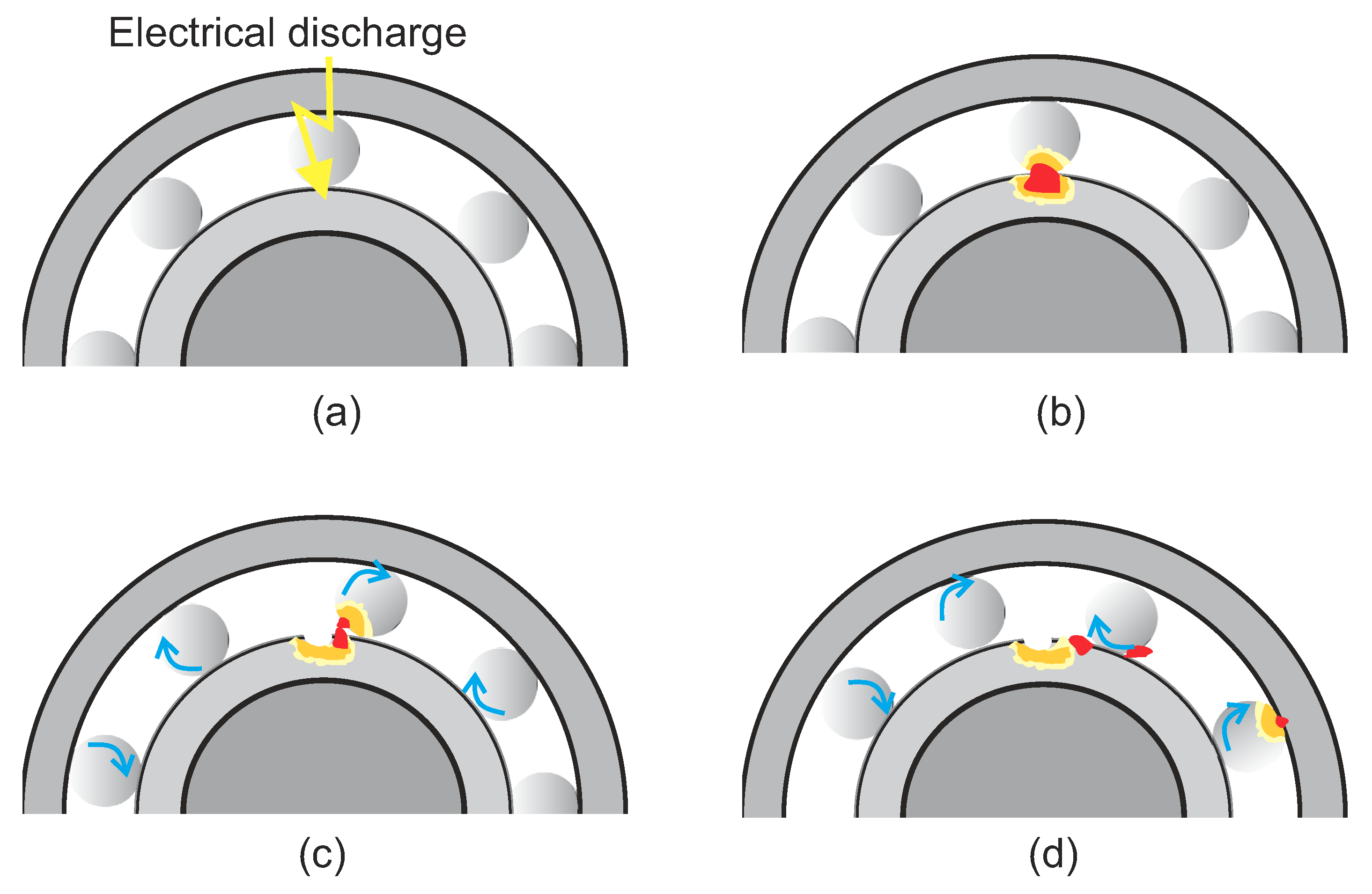
2.1. Bearing Faults Due to Electrical Arcing in Electric Motors

The most common reported failures linked to bearings are generally due to excessive loads, insufficient lubrication, external contamination, improper installation, and electrical arcing. This last has been considered a critical issue that can lead to the appearance of faults in bearings [29]. The presence of electrical arcing on the bearing elements is considered a phenomenon produced by the current leakage, which generates a micro-scaling of the rolling surfaces [4]. This current leakage may generate small craters on the bearing surfaces (outer and/or inner races) as the leakage of currents travels through the rolling elements (bearing balls) from the outer race to the inner race, as depicted in Figure 1a. This leakage current on a small contact surface may produce an arc-welding process, characterized by the presence of high temperatures as shown in Figure 1b. Consequently, as the material is heated, it may reach melt temperatures where the melted material may be easily removed and taken away due to the rotation of the rolling elements (bearing balls), see Figure 1c,d. As a consequence, the craters produced in the outer race of the bearing may lead to the generation of irregular contact surfaces, causing an impact each time the bearing elements pass through them.

2.2. Rolling Bearing Faults and Its Relationship with Stray Flux Signals

As reported in the literature, it is known that bearing defects generate mechanical impact produced by the rolling elements over the bearing race. When the bearing defect is located in the outer race it will cause an impulse each time the rolling elements contact the irregularity, causing a modulation effect, which can sometimes be observed in the vibration signals [6]. This modulation gives rise to characteristic frequencies related to the rotor rotational frequency ( f r ) and the bearing geometry, and for the case of outer-race faults these frequencies ( f BPOF ) are given by (1).
f BPOF = f r 2 · N b · 1 + D B D C cos ( θ )
where D C is the cage diameter measured from a ball center to the opposite ball center, D B is the ball diameter, N b is the number of balls, and θ is the contact angle between the bearing surfaces.
The vibration component effect on the current has been linked and modeled according to two main approaches. On the one hand, the vibration component at one of the fault characteristic frequencies is considered to act on the electric machine as a torque ripple that produces a speed ripple. Consequently, the vibration is reflected in the current as a group of side-band components ( f B E ) of the power supply frequency ( f s ) given by (2) [20]:
f BE = f s ± k · f BPOF
where k is a positive integer.
On the other hand, the effect of the vibration component on the current is modeled as a static eccentricity, which cause the amplification of f BE frequencies. Moreover, as referred in [30], the stray flux of an electric motor is the magnetic flux that radiates outside the frame of the machine, induced by stator and rotor currents. These currents (and hence the stray flux) are modified when the electric motor operates under a fault condition. Then, as shown in [22], specific frequencies are amplified in the stray flux signals when there is a bearing fault. However, the amplification of such frequencies are very low, which makes the diagnosis a challenging task, directing the researches towards novel methodologies not dependent on specific frequencies.
As reported in [30], the stray flux can be analyzed through its two magnetic components: axial and radial stray flux. Such magnetic signals may be acquired by installing suitable sensors on the frame of the motor at specific positions. Figure 2 shows the presumed circulation of the field lines of the axial and radial stray fluxes. In this way, the axial field can be measured by installing a proper sensor at position 1, the radial field through position 3 and position 2 captures a combination of both stray fluxes.

2.3. Linear Discriminant Analysis

The linear discriminant analysis (LDA) is a very common supervised dimensionality reduction technique that is generally used as a pre-processing step for machine learning and pattern classification applications purposes. The main objective of this classifier technique is focused to project a dataset of d-dimensional vectors onto a smaller subspace s (where s d ) by maximizing the linear separability between data of different classes finding a linear mapping [31]. This technique has been widely applied in classic feature reduction approaches to obtain a new non redundant set of less features in such a way that a combination of relevant information provided by different indices is carried out. Hence, despite a specific feature does not provide meaningful information by itself; it can provide relevant information by its combination with other [3]. The mathematical procedure to perform LDA is described in summary below and can be found in detail in different literature as in [32]:
  • Compute d-dimensional mean vectors of the input matrix
  • Compute between-class matrix and within-class scatter matrix.
  • Compute eigenvectors and eigenvalues.
  • Select linear discriminants for the new feature subspace and form an eigenvector matrix.
  • Use the eigenvector matrix to transform the vectors onto the new lower dimensional space.
  • Maximize the between-class matrix and minimize within-class scatter matrix.

2.4. Statistical Time-Domain Features

The main objective of statistical time-domain features (TF) is to obtain relevant information about the behavior of a system by means of a time-signal. Since a system with different operating conditions has signals with variated statistical parameters, it is expected that a system working under a fault condition will reflect its status on such features [33]. Statistical time-domain indices such as mean, root mean square (RMS), standard deviation, variation, impulse factor, shape factor, among others have been successfully used for the condition monitoring of electric machines [28,33,34]. The low computation burden and memory resources used to compute them, the capability to bring information about general trends, and its simplicity have allowed its proliferation for diagnosis schemes intended for online diagnosis and its implementation on hardware [35]. On the other hand, higher dimensional features such as kurtosis, and skewness examine the probability density function (PDF) of the time-domain signal in order to bring information able to characterize any difference encountered on distinct PDF. In this way a time-domain signal may be successfully characterized by a set of several time-domain features. In this work it is considered a set of 15 TF, whose mathematical formulation is described in Table 1, where x k is the time-domain signal for k = 1 , 2 , , N with N being the number of data points.
In order to keep only the most representative TF and minimize redundancy problems, a posterior pre-processing stage is performed by applying the Fisher score technique. This method may be interpreted as a relative measurement which represents the distance between different classes and dispersion among data points belonging to each class. In this way, a small Fisher score (FS) implies poor discriminative capability, while a larger Fisher score links a better discriminative feature. Considering this, the feature selection is performed under a combinatorial approach where the Fisher scores are obtained by carrying out combinations between all the available statistical features. Hence, the discriminative capabilities are evaluated by considering different subsets of features. Then, after evaluating the Fisher score of each subset of statistical features, the first ranked subset is considered as the most relevant and discriminative. The FS j of the j feature is given by (3) [34].
FS j = i = 1 c n i μ i j μ j 2 i = 1 c n i σ i j 2
where μ i j , σ i j , and n i are the mean, standard deviation, and size of ith c-class of the jth feature, respectively, μ j is the mean of the whole data set of the jth feature.
Table 1. Statistical time-domain features.
FeatureEquation FeatureEquation
Mean x ¯ = 1 N · k = 1 N x k (4)Crest factor C F = m a x ( x ) R M S (5)
Root mean square R M S = 1 N · k = 1 N ( x k ) 2 (6)Latitude factor L F = m a x ( x ) S R M (7)
Square root mean S R M = 1 N k = 1 N x k 2 (8)Impulse factor I F = m a x ( x ) 1 N · k = 1 N x k (9)
Standard deviation σ = 1 N k = 1 N x k x ¯ 2 (10)Skewness S k = k = 1 N x k x ¯ 3 N · σ 3 (11)
Variance σ 2 = 1 N k = 1 N x k x ¯ 2 (12)Kurtosis k = k = 1 N x k x ¯ 4 N · σ 4 (13)
RMS shape factor S F R M S = R M S 1 N · k = 1 N x k (14)Fifth central momenth 5 t h M = k = 1 N x k x ¯ 5 N · σ 5 (15)
SRM shape factor S F S R M = S R M 1 N · k = 1 N x k (16)Sixth central moment 6 t h M = k = 1 N x k x ¯ 6 N · σ 6 (17)

2.5. Fractal Dimension Analysis

Fractal dimension (FD) analysis is a concept of chaos theory, which attempts to measure the amount of self-similarity or repeated patterns that are present in a time-domain signal [36]. The fractal characterization may be especially useful for analyzing and comparing complex waveforms [37]. In this way, a FD analysis may be used to assess the consistency of a time-domain signal, which inherently implicates that such analysis may yield information related to the variations that modify the regularity of a signal. Therefore, extrapolating these ideas for the case of bearing faults in stray flux signals, it is expected an alteration in the measured signal due to a bearing fault (amplitude increase of fault-related frequencies or transient characteristics in the measured signal), which can vary according to the severity of the damage, such change may be characterized by a fractal index. A fractal dimensions of a time-domain signal may range from 1.0 for straight lines to 2.0 according to the complexity and self-similarity. Katz’s FD measures the fractality of a time-series signal x by means of the Euclidean distance of successive data points. Its simple computation and low computational resources make Katz’s FD optimal be implemented on hardware for online-intended schemes. The mathematical procedure to obtain Katz’s FD is as follows:
  • Find the maximum Euclidean distance d between the first sample x 1 and sample x k (for k = 1 , , N ), N represents the number of samples found in the time-domain signal).
  • Obtain the arithmetic sum of the Euclidean distances (L) between successive samples of time-domain signal x and then calculate its average (a) as follows:
    L = k = 2 N distance ( x k x k 1 )
    a = L N 1
  • Compute the fractality, KFD, of the time-domain series signal according to Equation (20):
    KFD = log ( L / a ) log ( d / a )

3. Proposed Methodology
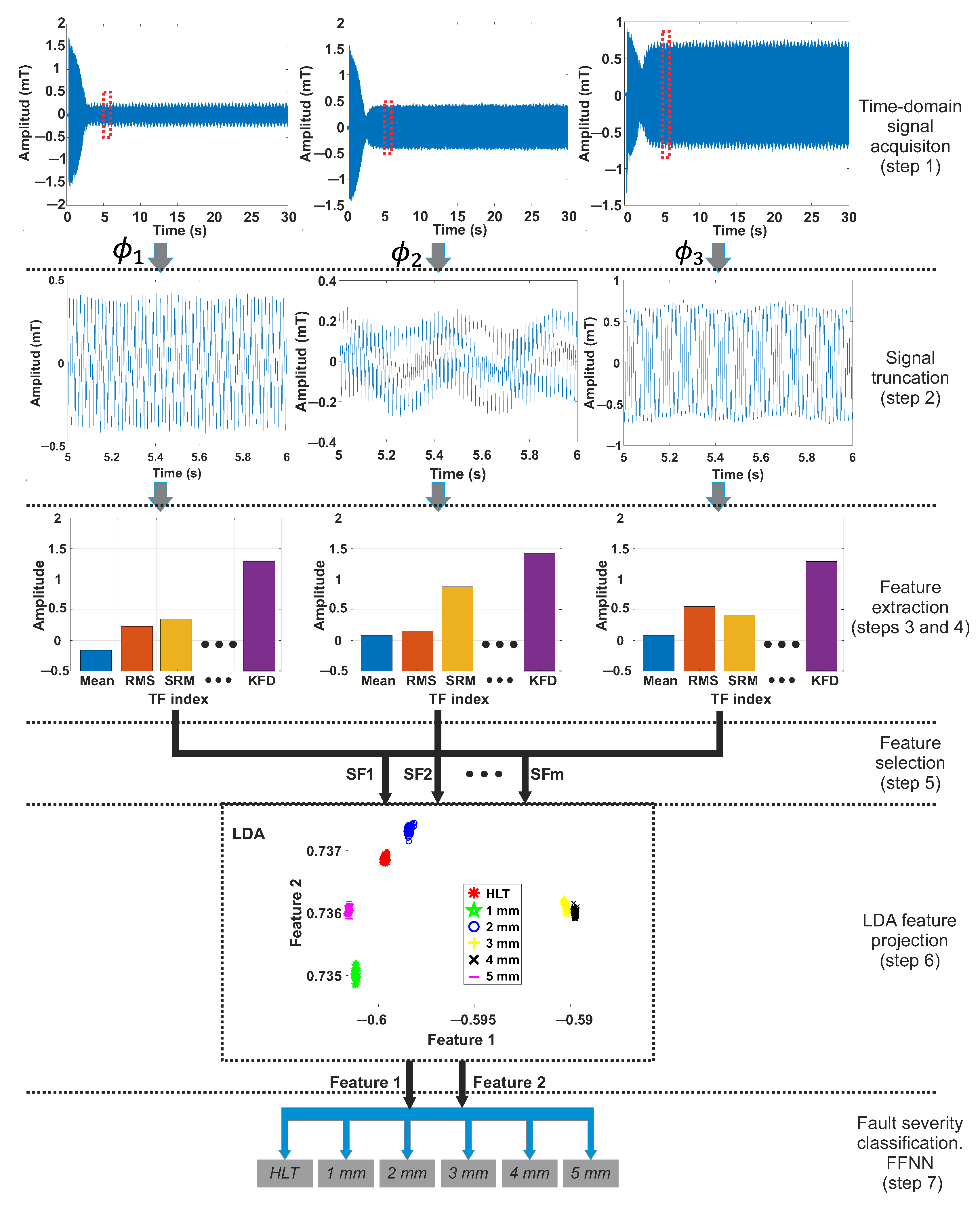
The proposed methodology (shown in Figure 3) for diagnosing a gradual wear on the outer race of rolling bearings by means of stray flux signals is mainly composed by seven steps as follows:
Step 1.
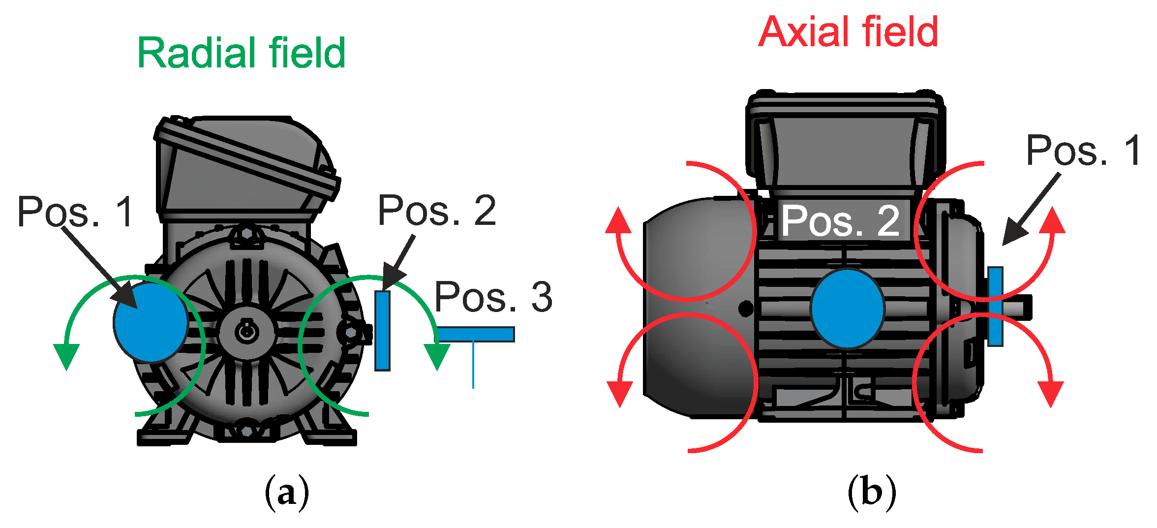
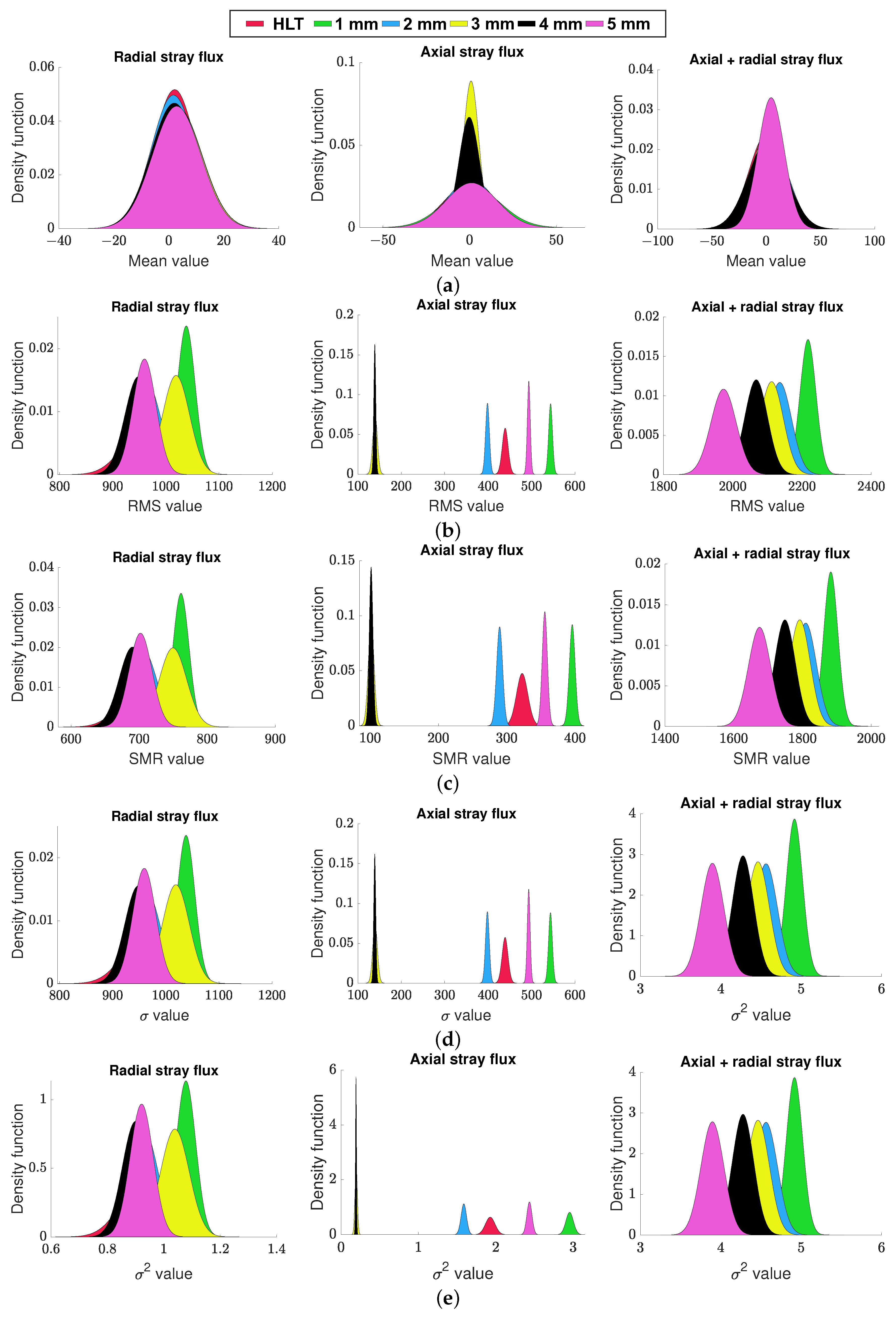
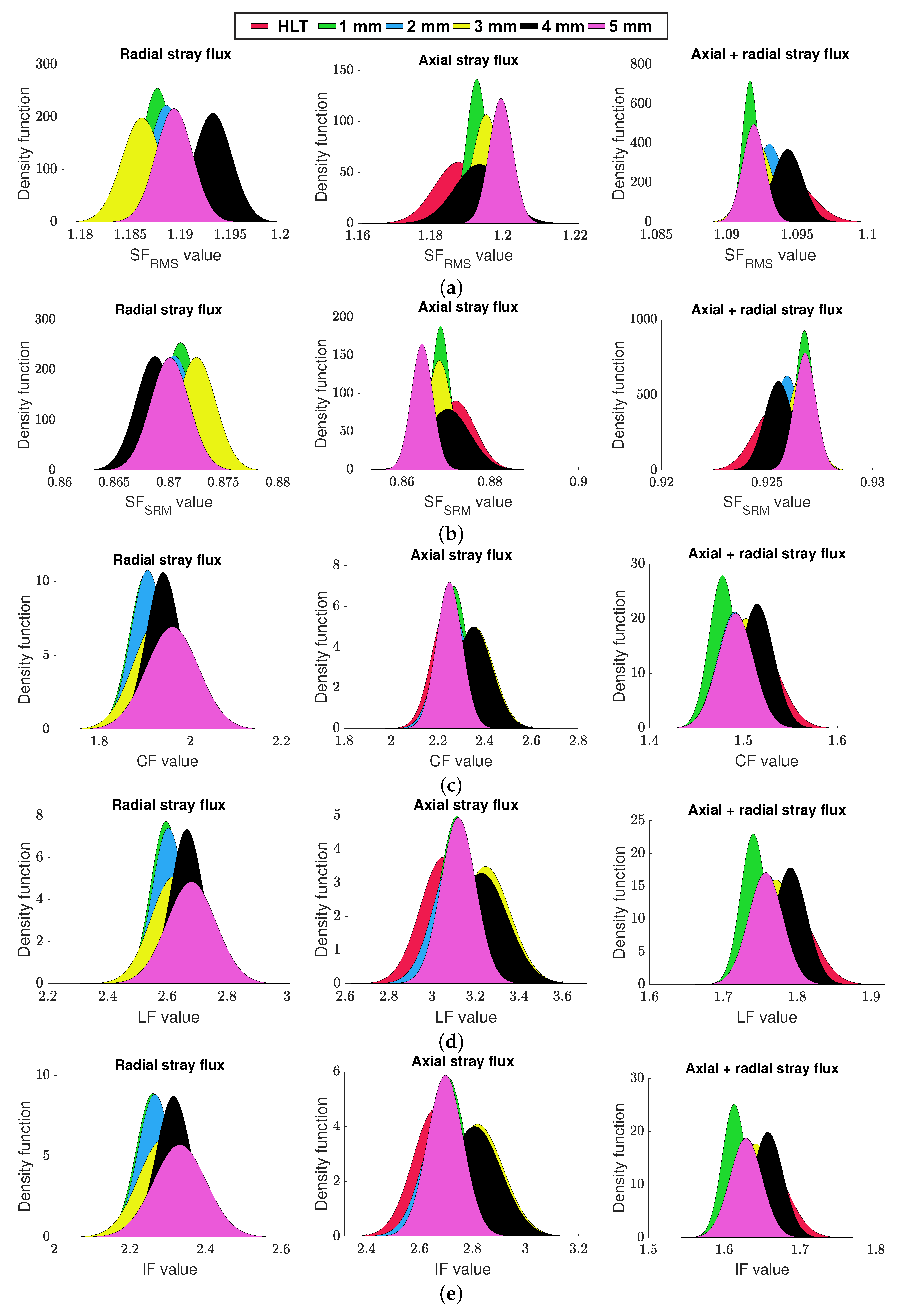
Acquire the different time-domain stray flux signals encountered around the driving motor, namely: radial stray flux ( ϕ 1 ), axial stray flux ( ϕ 2 ), and axial + radial stray flux ( ϕ 3 ).
Step 2.
Proceed to extract a truncated signal (for each stray flux acquired component) by means of a rectangular windowing centered at the steady state of the machine. A minimum size of 1 s time length is recommended in order to reduce the effect of processing noise produced by external sources.
Step 3.
Feature extraction. Calculate the different statistical time-features described in Section 2.4 according to the corresponding equations listed in Table 1.
Step 4.
Compute the Katz’s fractal dimension as described in Section 2.5 by applying Equation (20), and add it to the complete set of time-domain features.
Step 5.
Perform a feature selection in order to segregate the m number of most significant and discriminative TF (SF1, SF2, …, SFm). Using (3) evaluate the discriminative capabilities of all the calculated TF by carrying out combinations between all the available statistical features and retain the ones with the highest Fisher score.
Step 6.
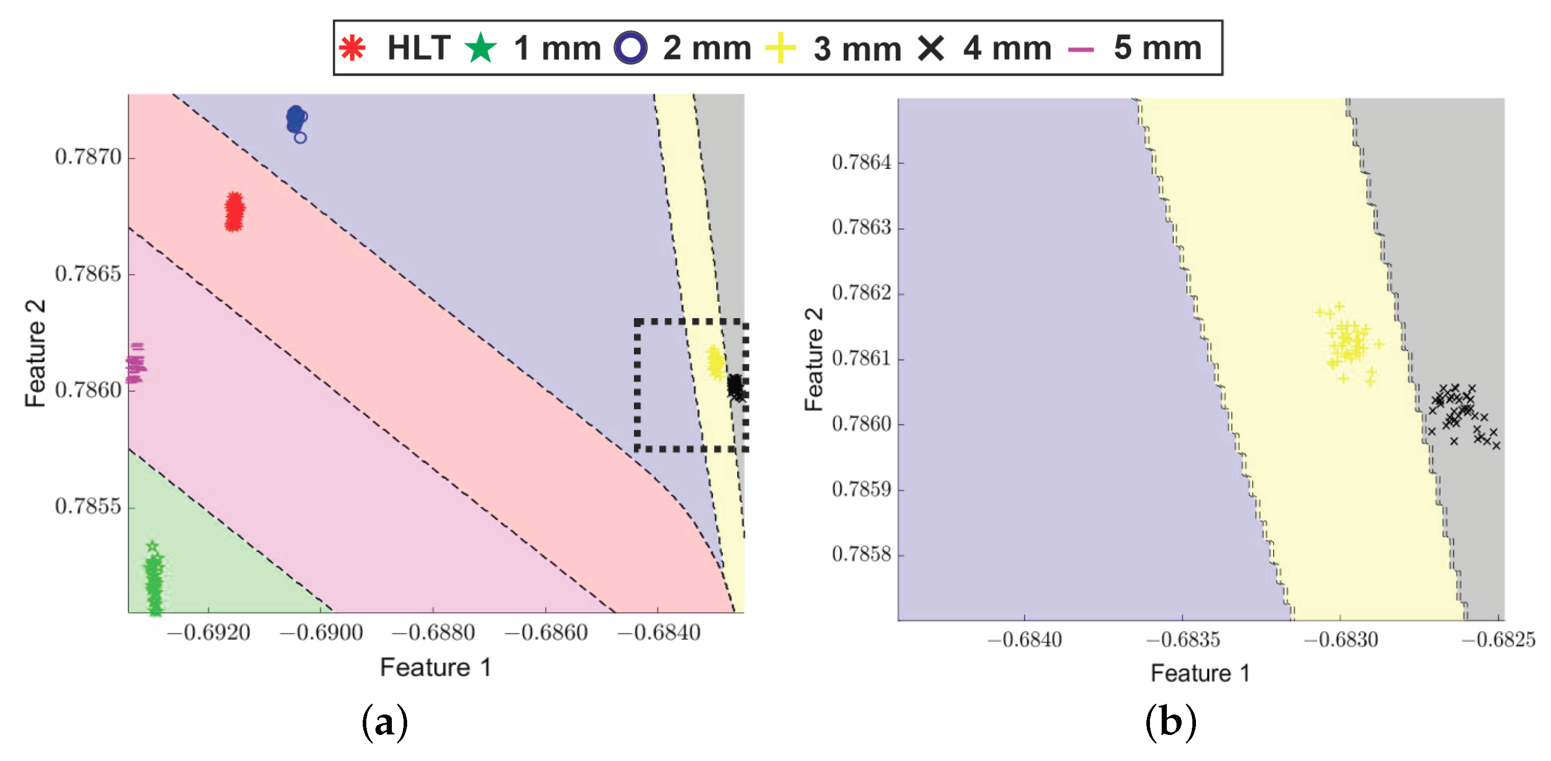
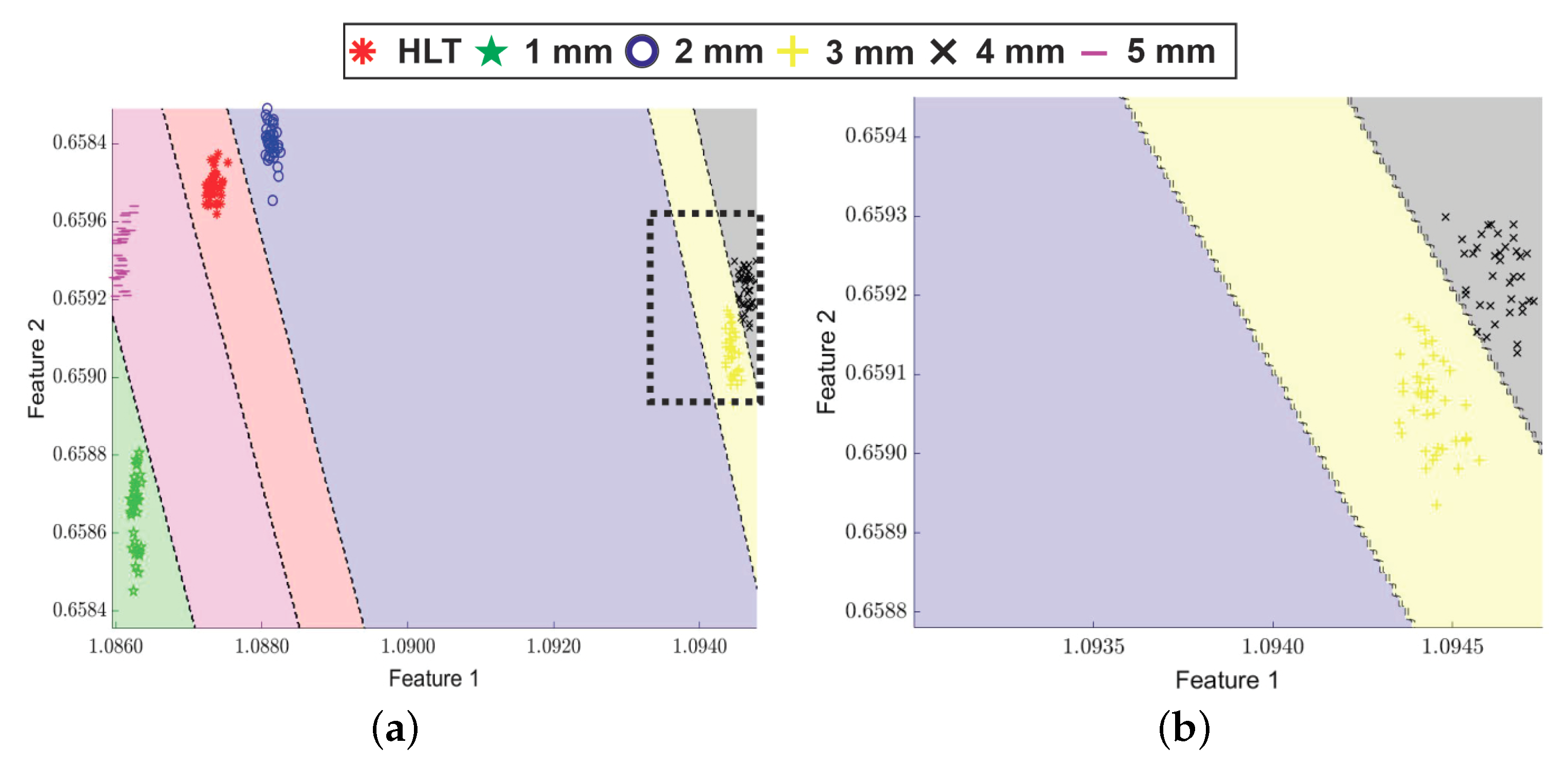
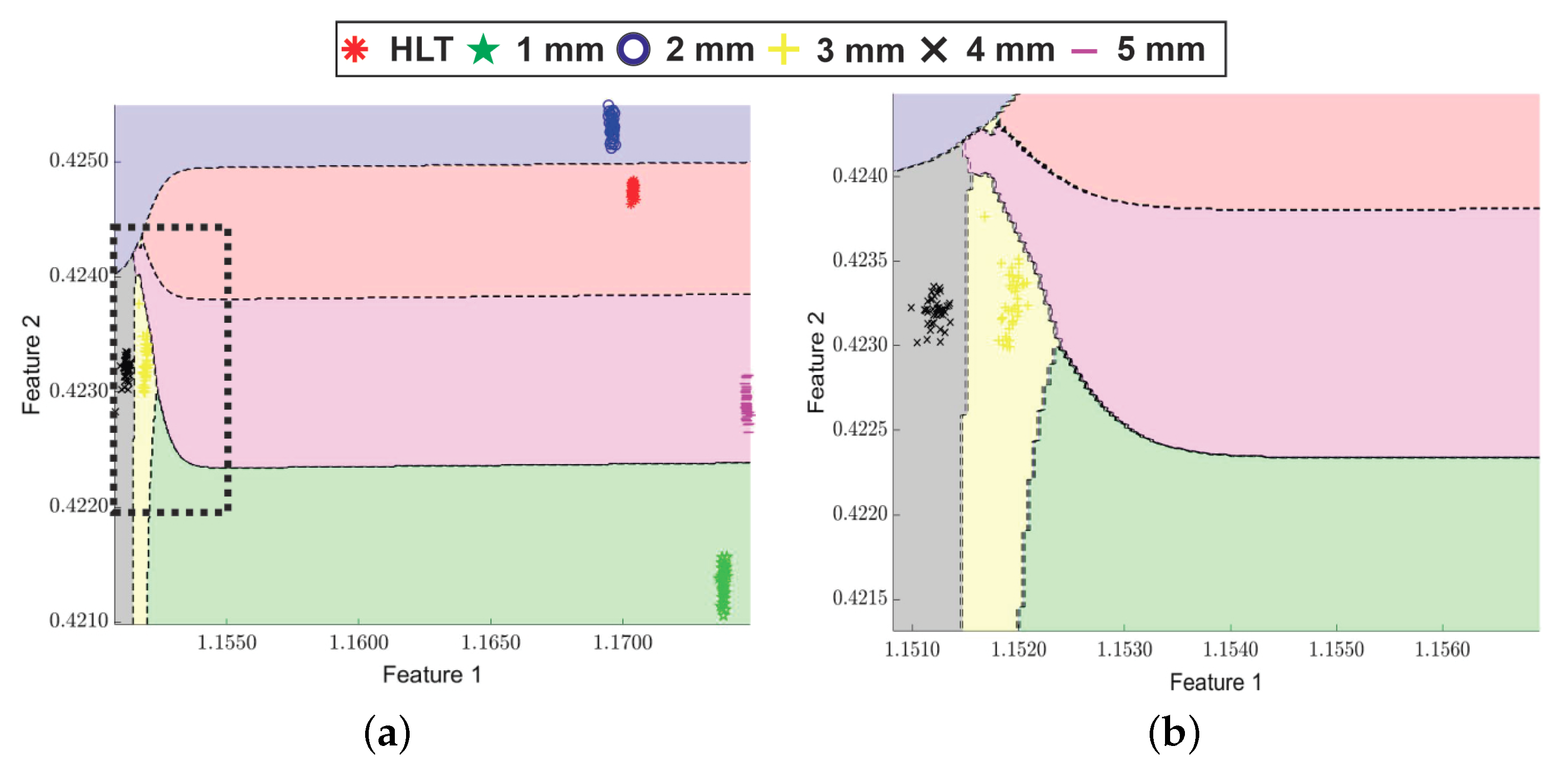
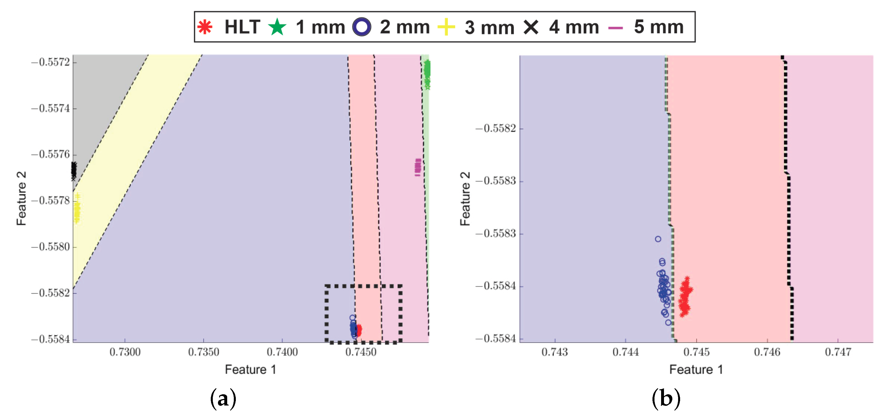
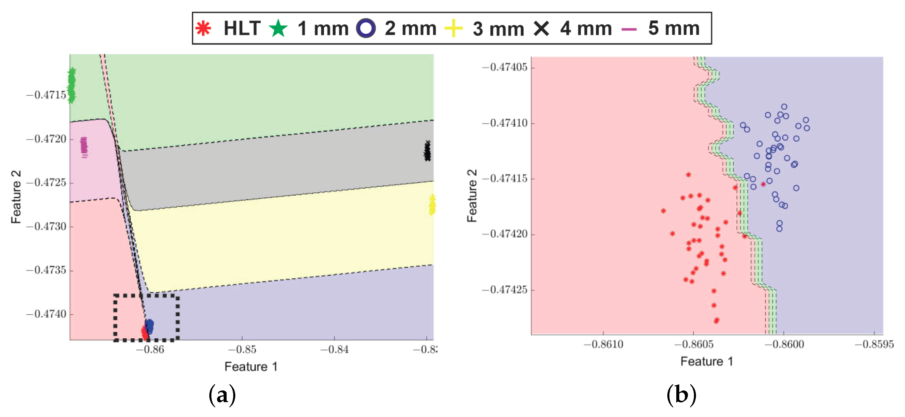
Carry out a feature reduction by applying a LDA in order to combine relevant information yielded by the selected most discriminative features, and obtain a transformation to 2 final features (Feature 1, and Feature 2). After that, a two-dimensional projection is obtained, where the Euclidean distance among different fault severities is maximized. This projection allows to observe the data clustering between different fault severities as the main projection axis are selected to be Feature 1 and Feature 2, respectively.
Step 7.
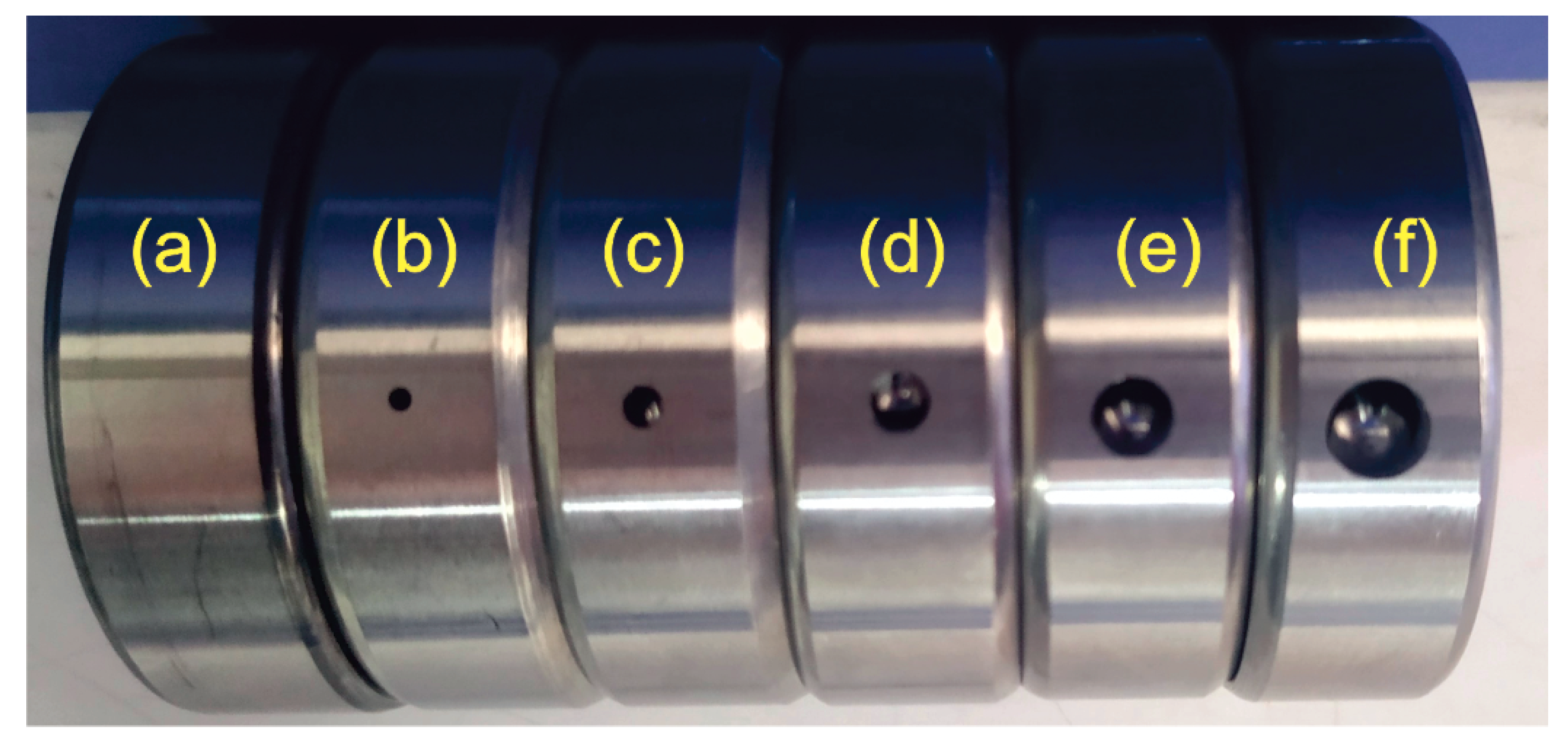
Classify the bearing fault severity. For the objectives of this paper, it is used a FFNN with hyperbolic tangent sigmoid and linear activation functions in the hidden and output layers, respectively, which allows for an easy learning [38]. This architecture is selected due to its simplicity, high performance as an automatic classifier, and the low computation resources demanded for its computation. The features obtained after the linear discriminant analysis are feed to the FFNN, which is trained to classify among the different studied faults. In this paper, these classes correspond to healthy bearing (HLT), 1 mm, 2 mm, 3 mm, 4 mm, and 5 mm hole diameter in the outer race as fault.
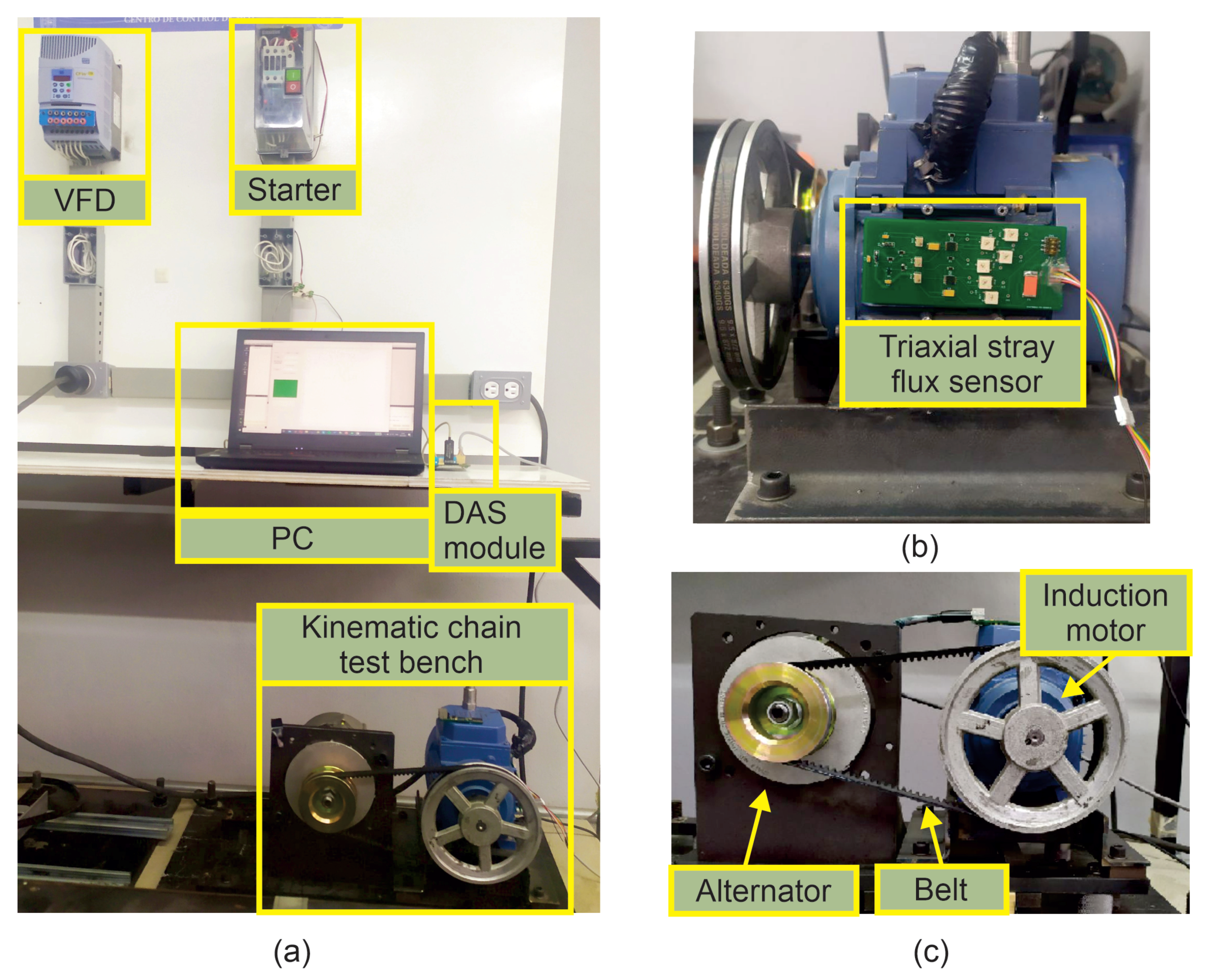
Experimental Setup

The validation of the proposed methodology is performed by analyzing several signals acquired from a kinematic chain test bench. The used kinematic chain is composed by an induction motor, a belt and pulleys transmission system and a mechanical load provided by an alternator, which represents 25% of the nominal load (see Figure 4c). The analyzed three-phase induction motor (model WEG 00136APE48T) has 2 poles, 28 bars, and a nominal power of 0.746 KW. It is fed with 220 Vac at 60 Hz for a direct start by means of an starter. Additionally, in order to validate the proposed method for different supply frequencies, the rotational speed is controlled by means of a VFD model WEG CFW08, which can be observed in Figure 4a. The stray flux signals are captured by means of a triaxial stray flux sensor (which is essentially compound by three individual Hall-effect transducers located on perpendicular axis to each other) installed on the data plate, as shown in Figure 4b. The stray flux signals are acquired by means of a proprietary data acquisition system (DAS) module, and then stored on a personal computer (PC) for their processing. The DAS module uses a 14 bit analog to digital converter, the sampling frequency is set at 5 KHz, and the signals are acquired within a period of 30 s, which is enough to capture the transient start up and at least 20 s of steady state. In order to obtain a significative number of tests, 7 different signals were obtained for each case study, as indicated in Table 2. In this regard, a total of 210 samples are collected during testing.
The experiments are carried out using different metallic bearings model 6203 2RS as the one shown in Figure 5. This bearing has 8 balls, 40 mm of external diameter (D) and 17 mm in the inner diameter (d). The outer race rolling bearing fault is induced through a milling machining process by drilling a hole on the outer race of the different bearings using a tungsten drill bit. In this way, an outer race gradual wear is induced for the different hole diameters as follows: 1 mm, 2 mm, 3 mm, 4, and 5 mm (see Figure 6). In all the considered faults, the experiments are carried out by replacing the healthy bearing with each one of the damaged bearings.
The FFNN is trained through the Levenberg-Marquardt algorithm for identifying among the different case studies. For this, a total of 140 windowed signals are extracted from the measurements per each condition state: 7 (acquired signals) by 20 (windowed signals). Each windowed signal is taken from a time window of 1 s (with no overlapping) when the machine reaches steady state. From the 140 signals obtained per each condition state (classification goal), 100 are used for training, and 40 for validation. The FFNN final architecture has 2 inputs (feature 1, and feature 2), 2 and 8 neurons in the hidden layers, and 6 outputs (one per each bearing condition).

4. Results

Following the proposed methodology, the stray flux signals responses for each bearing condition (i.e., healthy bearing, 1 mm, 2 mm, 3 mm, 4 mm, and 5 mm outer race hole diameter) are analyzed. Hence, the proposal is carried out for each power supply frequency studied here (i.e., 60 Hz direct line, and 60 Hz, 50 Hz, 15 Hz, and 5 Hz VFD connection).
Figure 7 shows graphically the normalized density functions defining detectability zones obtained by the mean, RMS, SMR, σ , and σ 2 values for the case when the driving motor is powered at 60 Hz under a direct line connection. In this way, Figure 7a reveals that the mean value does not provide any discriminative data since all the fault severities exhibits an overlapping. In a similar fashion, Figure 7b–e demonstrates that RMS, SMR, σ , and σ 2 may bring relevant discriminative information for the different fault severities (as there is a low overlapping among them). On the other hand, Figure 7 shows that by means of the RMS, SMR, σ , and σ 2 time-domain features it is possible to individually discriminate among healthy, 1 mm, 2 mm, and 5 mm fault severities since there is almost a null overlapping on all these cases (when analyzing the axial stray flux). In addition, Figure 8a–e indicates the poor discriminative performance obtained by the SF R M S , SF S R M , CF, LF, IF when analyzed individually, since there is an overlapping in all the cases. Finally, Figure 9a,c indicates that there is almost a null discriminative data in the S k , and 5 t h M time-domain features when the driving motor is powered at 60 Hz under a direct line connection. Nonetheless, Figure 9e demonstrates the relevance of including the KFD feature (specially for the axial stray flux signal), since it shows a low overlapping among the different fault severities. To this end, it is worth noting that a final diagnosis can not be carried out by the direct evaluation of a single TF value, since an undesired false indication may be obtained as an overlapping among different fault severities is obtained.
In order to select the most discriminative set of features, a three-feature combination subset is generated for each study case (the same three-feature subset combination is considered for the different acquired stray flux signals). Subsequently, these subsets are evaluated through the Fisher score, which is computed by applying (3), and the best combination is selected, i.e., the subset with the highest Fisher score values. Table 3 summarizes the subsets of TF and KFD features with the highest FS values. It can be clearly seen that the combination of σ , k, KFD, S F R M S , S F S R M , 5 t h M , 6 t h M , and SMR performs best for discriminating the faults when the driving motor is powered at 60 Hz under a direct line connection. Similarly, the best combination of features for diagnosing outer race bearing faults when the driving motor is powered at 60 Hz by a VFD turns to be compound by the RMS, SRM, σ , S F R M S , S F S R M , KFD, mean, and σ 2 . On the other hand, the best discriminative performance under a 50 Hz VFD connection is found to be linked to the RMS, SRM, k, S F R M S , S F S R M , and KFD as stated in Table 3. In a similar fashion, Table 4 compiles the best TF which brings more discriminative information for the diagnosis of bearing faults when powering the driving motor at 15 Hz, and 5 Hz.
After that, in the last stage of the proposed methodology, a feature extraction is performed by a LDA, in which all the selected statistical features are projected into a small subset in order to maximize the linear separation between different classes by combining the information provided by different TF values. Consequently, the extracted set of features is projected into a 2-dimensional space in order to obtain a visual representation of all the considered conditions. In this regard, Figure 10a depicts the resulting classification performances reached during the training and test of the FFNN classifier for the different bearing damages when the driving motor is powered at 60 Hz under a direct line connection. Besides, Figure 10b provides a zoomed view of a critical zone (where the separation between classes is smaller). From this Figure, it can be clearly seen that the dispersion obtained for the different fault severities is minimal, and the separation between classes is large. In a similar fashion, Figure 11a shows the correct classifications and boundaries automatically obtained by means of the FFNN for the case when the driving motor is powered by a VFD at 60 Hz. Additionally, Figure 11b (which is a zoomed view of the black rectangle zone found in Figure 11a) reveals that there is no overlapping, or misclassification between 3 mm, and 4 mm fault severities despite being in a closely located region. Similar results can be appreciated from Figure 12 and Figure 13. With regards to the decision boundaries and obtained projection when the driving motor is powered at 5 Hz, Figure 14 shows that there is a misclassification between the healthy baring and 2 mm faulty bearing, since the projected data turns to be in very closely regions. Nevertheless, the both cases are accurately separated.
Table 5 shows the classification results, as well as the effectiveness percentage of the proposed methodology when the driving motor is powered at 60 Hz (direct line), and 60 Hz, 50 Hz, and 15 Hz by means of a VFD. Correct classifications are located in the diagonal of the Table (highlighted in bold). The effectiveness, per bearing state, is obtained through the calculation of the fault detection rate index (FDR) by dividing the number of correct classifications over the total number of samples. These results demonstrates the relevance of the proposal since a correct fault severity classification of 100% is obtained, even for incipient faults. Similarly, Table 6 shows the confusion matrix obtained for the case when the driving motor is powered by a VFD at 5 Hz. This special case reveals that the proposal has an effectiveness of 97.5% for classifying bearing faults under incipient stages, even when the rotor rotational speed is very slow. The classification and fault diagnosis at very slow rotor rotational speeds by means of conventional techniques turns to be very difficult, since the fundamental harmonic (which has a high amplitude) overlaps to adjacent components.

5. Discussion

It can be clearly seen from Figure 7, Figure 8 and Figure 9 (which show graphically the normalized density functions defining detectability zones obtained by each TF, and KFD) that there is a grade of overlapping between the different fault severities studied here when evaluating a single time feature. This overlapping exhibit that a final diagnosis can not be carried out by the direct evaluation of a single TF value, since an undesired false indication may be obtained. On the other hand, Figure 10, Figure 11, Figure 12, Figure 13 and Figure 14 evidence that it is possible to correctly separate and classify among the different faults studied here by combining the information yielded by the most discriminative TF when using a suitable technique (such as LDA), which turns to be fundamental for the final diagnosis. In addition, these Figures shows that even though some classification regions, such as 5 mm region is near to the healthy zone, there is no overlapping as the distance between them turns to be large enough to allow the FFNN to correctly classify among the different fault severities. The non-linear behavior obtained on the results can be mainly attributed to the time-features used to characterize the kinematic chain under study, as they provide relevant information about changes and trends found in the analyzed signals. Such changes are found to be no linear to the fault severity.
Moreover, it is found from the obtained results, that different subsets of time-domain features brings relevant discriminative information for diagnosing bearing faults according to the different power supply frequencies studied here. However, the total features used to discriminate all the bearing fault severities under different power supply frequencies is found to be confined to the following ones: σ , k, KFD, S F S R M , S F R M S , 5 t h M , 6 t h M , SMR, RMS, and σ 2 as stated in Table 3 and Table 4. Additionally, the information showed in Table 3 and Table 4 reveals that the Katz’s fractal dimension and σ turns to be indispensable for a correct fault severity classification, as these TF are found in almost all the subsets having the most higher FS values. Regarding the effectivenesses of the proposed methodology, Table 5 reveals that a 100% fault classification performance is obtained, even for incipient fault stages for the cases when the driving motor is powered at 60 Hz, 50 Hz, and 15 Hz. The worst classification results are obtained when the driving motor is powered under a very slow rotor rotational speed; since a misclassification of a healthy bearing is obtained as shown in Table 6. However, the proposed methodology turns to be feasible, since in this special case (i.e., very slow rotor rotational speed) conventional methodologies are not able to discriminate a fault considering that the fundamental harmonic (which has a high amplitude) overlaps to adjacent components. On the other hand, the triaxial stray flux sensor used (capable of capturing the different magnetic flux components from a single point) enables to acquire and characterize the different stray flux components from practically anywhere on the motor frame, thus avoiding errors due to sensor alignment and installation.
Finally, it should be mention that other damages such as broken rotor bars, load unbalance, among others, may yield different stray flux signals. Then, the performance of the classification method may be deteriorated and a new training for known conditions will be required. In this regard, a further research may be directed towards the addition of more faults in order to avoid false diagnosis due to unknown conditions.

6. Conclusions

This paper has proposed a non-invasive automatic methodology for the gradual wear diagnosis of outer race bearing faults by means of stray flux signals, time-domain features (TF) and machine learning methods. It has been shown the feasibility of analyzing different TF, and the Katz’s fractal dimension (KFD) for linking relevant information related to bearing faults. According to the obtained results, there is no individual TF able to discriminate among the different gradual wears studied here; however, with the combination of the information provided by distinct TF and the KFD by means of a linear discriminant analysis (LDA) it is possible to reliable classify and diagnose different wear severities. The proposed methodology overcomes a main drawback found in conventional methods since it does not require prior knowledge related to the installed bearing or the rotor rotational speed information. As shown in the obtained results, the proposal is able to automatically diagnose the different bearing fault severities studied here with a 100% effectiveness for the cases when the driving motor is powered at 60 Hz, 50 Hz, and 15 Hz, and a 97.5% correct classification is obtained when the driving motor is powered a at 5 Hz. From these results, it is evident that the proposal is a suitable and reliable methodology for the automatic detection of gradual wear bearing damages. In addition, the final diagnosis is not affected by low-amplitude signals, a main constraint encountered in some methods. The proposal may found a wide applicability on online schemes with the capability to detect incipient faults. The main constraint of the proposal is the requirement of enough data for the different case studies in order to perform an adequate training of the method.

Author Contributions

Conceptualization, I.Z.-R. and R.A.O.-R.; methodology, J.-J.S.-D., I.Z.-R. and J.A.A.-D.; validation, J.C.-O. and I.Z.-R.; formal analysis, I.Z.-R. and R.A.O.-R.; investigation, J.A.A.-D. and J.-J.S.-D.; resources, J.A.A.-D.; data curation, J.C.-O. and J.-J.S.-D.; writing—original draft preparation, I.Z.-R.; writing—review and editing, I.Z.-R., R.A.O.-R. and J.A.A.-D.; visualization, J.C.-O. and J.-J.S.-D.; supervision, J.-J.S.-D., R.A.O.-R. and J.A.A.-D.; project administration, J.A.A.-D. and R.A.O.-R.; funding acquisition, J.A.A.-D. All authors have read and agreed to the published version of the manuscript.

Funding

This work was supported by the Spanish ‘Ministerio de Ciencia Innovación y Universidades’ and FEDER program in the framework of the ‘Proyectos de I+D de Generación de Conocimiento del Programa Estatal de Generación de Conocimiento y Fortalecimiento Científico y Tecnológico del Sistema de I+D+i, Subprograma Estatal de Generación de Conocimiento’ (ref: PGC2018-095747-B-I00), and Consejo Nacional de Ciencia y Tecnología (CONACyT) under scholarship 652815.

Data Availability Statement

The data presented in this study are available on request from the corresponding author. The data are not publicly available due to other researches are in process using same data.

Conflicts of Interest

The authors declare no conflict of interest.

References

  1. Haraguchi, N.; Cheng, C.F.C.; Smeets, E. The importance of manufacturing in economic development: Has this changed? World Dev. 2017, 93, 293–315. [Google Scholar] [CrossRef]
  2. Bonnett, A.H.; Yung, C. Increased efficiency versus increased reliability. IEEE Ind. Appl. Mag. 2008, 14, 29–36. [Google Scholar] [CrossRef]
  3. Saucedo-Dorantes, J.J.; Delgado-Prieto, M.; Ortega-Redondo, J.A.; Osornio-Rios, R.A.; Romero-Troncoso, R.D.J. Multiple-fault detection methodology based on vibration and current analysis applied to bearings in induction motors and gearboxes on the kinematic chain. Shock Vib. 2016, 2016, 5467643. [Google Scholar] [CrossRef]
  4. Oliver, J.A.; Guerrero, G.; Goldman, J. Ceramic bearings for electric motors: Eliminating damage with new materials. IEEE Ind. Appl. Mag. 2017, 23, 14–20. [Google Scholar] [CrossRef]
  5. Frosini, L. Novel Diagnostic Techniques for Rotating Electrical Machines? A Review. Energies 2020, 13, 5066. [Google Scholar] [CrossRef]
  6. Trajin, B.; Regnier, J.; Faucher, J. Comparison between vibration and stator current analysis for the detection of bearing faults in asynchronous drives. IET Electr. Power Appl. 2010, 4, 90–100. [Google Scholar] [CrossRef] [Green Version]
  7. Zhang, S.; Zhang, S.; Wang, B.; Habetler, T.G. Deep learning algorithms for bearing fault Diagnostics? A comprehensive review. IEEE Access 2020, 8, 29857–29881. [Google Scholar] [CrossRef]
  8. Blodt, M.; Bonacci, D.; Regnier, J.; Chabert, M.; Faucher, J. On-line monitoring of mechanical faults in variable-speed induction motor drives using the Wigner distribution. IEEE Trans. Ind. Electron. 2008, 55, 522–533. [Google Scholar] [CrossRef]
  9. Choudhary, A.; Goyal, D.; Shimi, S.L.; Akula, A. Condition monitoring and fault diagnosis of induction motors: A review. Arch. Comput. Methods Eng. 2019, 26, 1221–1238. [Google Scholar] [CrossRef]
  10. Glowacz, A. Acoustic fault analysis of three commutator motors. Mech. Syst. Signal Process. 2019, 133, 106226. [Google Scholar] [CrossRef]
  11. Osornio-Rios, R.A.; Antonino-Daviu, J.A.; de Jesus Romero-Troncoso, R. Recent industrial applications of infrared thermography: A review. IEEE Trans. Ind. Inform. 2018, 15, 615–625. [Google Scholar] [CrossRef]
  12. Choudhary, A.; Goyal, D.; Letha, S.S. Infrared Thermography-Based Fault Diagnosis of Induction Motor Bearings Using Machine Learning. IEEE Sens. J. 2020, 21, 1727–1734. [Google Scholar] [CrossRef]
  13. Delgado-Arredondo, P.A.; Garcia-Perez, A.; Morinigo-Sotelo, D.; Osornio-Rios, R.A.; Avina-Cervantes, J.G.; Rostro-Gonzalez, H.; Romero-Troncoso, R.D.J. Comparative study of time-frequency decomposition techniques for fault detection in induction motors using vibration analysis during startup transient. Shock Vib. 2015, 2015, 708034. [Google Scholar] [CrossRef] [Green Version]
  14. Corne, B.; Vervisch, B.; Derammelaere, S.; Cruz, S.M.; Knockaert, J.; Desmet, J. Single point outer race bearing fault severity estimation using stator current measurements. In Proceedings of the 2017 IEEE International Electric Machines and Drives Conference (IEMDC), Miami, FL, USA, 21–24 May 2017; pp. 1–7. [Google Scholar]
  15. Cui, L.; Li, B.; Ma, J.; Jin, Z. Quantitative trend fault diagnosis of a rolling bearing based on Sparsogram and Lempel-Ziv. Measurement 2018, 128, 410–418. [Google Scholar] [CrossRef]
  16. Bediaga, I.; Mendizabal, X.; Arnaiz, A.; Munoa, J. Ball bearing damage detection using traditional signal processing algorithms. IEEE Instrum. Meas. Mag. 2013, 16, 20–25. [Google Scholar] [CrossRef]
  17. Chen, C.C.; Liu, Z.; Yang, G.; Wu, C.C.; Ye, Q. An Improved Fault Diagnosis Using 1D-Convolutional Neural Network Model. Electronics 2021, 10, 59. [Google Scholar] [CrossRef]
  18. Zamudio-Ramirez, I.; Osornio-Rios, R.A.A.; Antonino-Daviu, J.A.; Razik, H.; de Jesus Romero-Troncoso, R. Magnetic Flux Analysis for the Condition Monitoring of Electric Machines: A Review. IEEE Trans. Ind. Inform. 2021. [Google Scholar] [CrossRef]
  19. Leite, V.C.; da Silva, J.G.B.; Veloso, G.F.C.; da Silva, L.E.B.; Lambert-Torres, G.; Bonaldi, E.L.; de Oliveira, L.E.D.L. Detection of localized bearing faults in induction machines by spectral kurtosis and envelope analysis of stator current. IEEE Trans. Ind. Electron. 2014, 62, 1855–1865. [Google Scholar] [CrossRef]
  20. Immovilli, F.; Bellini, A.; Rubini, R.; Tassoni, C. Diagnosis of bearing faults in induction machines by vibration or current signals: A critical comparison. IEEE Trans. Ind. Appl. 2010, 46, 1350–1359. [Google Scholar] [CrossRef]
  21. Lee, S.B.; Shin, J.; Park, Y.; Kim, H.; Kim, J. Reliable Flux based Detection of Induction Motor Rotor Faults from the 5th Rotor Rotational Frequency Sideband. IEEE Trans. Ind. Electron. 2020, 68, 7874–7883. [Google Scholar] [CrossRef]
  22. Vitek, O.; Janda, M.; Hajek, V.; Bauer, P. Detection of eccentricity and bearings fault using stray flux monitoring. In Proceedings of the 8th IEEE Symposium on Diagnostics for Electrical Machines, Power Electronics & Drives, Dallas, TX, USA, 22–25 August 2021; pp. 456–461. [Google Scholar]
  23. Frosini, L.; Harlişca, C.; Szabó, L. Induction machine bearing fault detection by means of statistical processing of the stray flux measurement. IEEE Trans. Ind. Electron. 2014, 62, 1846–1854. [Google Scholar] [CrossRef]
  24. Harlişca, C.; Szabó, L.; Frosini, L.; Albini, A. Diagnosis of rolling bearings faults in electric machines through stray magnetic flux monitoring. In Proceedings of the 2013 8th International Symposium on Advanced Topics in Electrical Engineering (ATEE), Bucharest, Romania, 23–25 May 2013; pp. 1–6. [Google Scholar]
  25. Luo, G.; Habetler, T.G.; Hurwitz, J. Stray Flux-Based Incipient Stage Bearing Fault Detection for Induction Machines via Noise Cancellation Techniques. In Proceedings of the 2020 IEEE Energy Conversion Congress and Exposition (ECCE), Detroit, MI, USA, 11–15 October 2020; pp. 764–768. [Google Scholar]
  26. Wang, D.; Tsui, K.L.; Miao, Q. Prognostics and health management: A review of vibration based bearing and gear health indicators. IEEE Access 2017, 6, 665–676. [Google Scholar] [CrossRef]
  27. Ewert, P.; Kowalski, C.T.; Orlowska-Kowalska, T. Low-Cost Monitoring and Diagnosis System for Rolling Bearing Faults of the Induction Motor Based on Neural Network Approach. Electronics 2020, 9, 1334. [Google Scholar] [CrossRef]
  28. Mao, W.; Wang, L.; Feng, N. A new fault diagnosis method of bearings based on structural feature selection. Electronics 2019, 8, 1406. [Google Scholar] [CrossRef] [Green Version]
  29. Plazenet, T.; Boileau, T.; Caironi, C.; Nahid-Mobarakeh, B. A comprehensive study on shaft voltages and bearing currents in rotating machines. IEEE Trans. Ind. Appl. 2018, 54, 3749–3759. [Google Scholar] [CrossRef]
  30. Romary, R.; Roger, D.; Brudny, J.F. Analytical computation of an AC machine external magnetic field. Eur. Phys. J. Appl. Phys. 2009, 47, 31102. [Google Scholar] [CrossRef]
  31. Song, X.; Liu, Z.; Yang, X.; Yang, J.; Qi, Y. Extended semi-supervised fuzzy learning method for nonlinear outliers via pattern discovery. Appl. Soft Comput. 2015, 29, 245–255. [Google Scholar] [CrossRef]
  32. Wen, J.; Fang, X.; Cui, J.; Fei, L.; Yan, K.; Chen, Y.; Xu, Y. Robust sparse linear discriminant analysis. IEEE Trans. Circuits Syst. Video Technol. 2018, 29, 390–403. [Google Scholar] [CrossRef]
  33. Caesarendra, W.; Tjahjowidodo, T. A review of feature extraction methods in vibration-based condition monitoring and its application for degradation trend estimation of low-speed slew bearing. Machines 2017, 5, 21. [Google Scholar] [CrossRef]
  34. Saucedo-Dorantes, J.J.; Delgado-Prieto, M.; Osornio-Rios, R.A.; Romero-Troncoso, R.D.J. Diagnosis methodology for identifying gearbox wear based on statistical time feature reduction. Proc. Inst. Mech. Eng. Part C J. Mech. Eng. Sci. 2018, 232, 2711–2722. [Google Scholar] [CrossRef] [Green Version]
  35. Huerta-Rosales, J.R.; Granados-Lieberman, D.; Garcia-Perez, A.; Camarena-Martinez, D.; Amezquita-Sanchez, J.P.; Valtierra-Rodriguez, M. Short-Circuited Turn Fault Diagnosis in Transformers by Using Vibration Signals, Statistical Time Features, and Support Vector Machines on FPGA. Sensors 2021, 21, 3598. [Google Scholar] [CrossRef] [PubMed]
  36. Amezquita-Sanchez, J.P.; Valtierra-Rodriguez, M.; Perez-Ramirez, C.A.; Camarena-Martinez, D.; Garcia-Perez, A.; Romero-Troncoso, R.J. Fractal dimension and fuzzy logic systems for broken rotor bar detection in induction motors at start-up and steady-state regimes. Meas. Sci. Technol. 2017, 28, 075001. [Google Scholar] [CrossRef]
  37. Katz, M.J. Fractals and the analysis of waveforms. Comput. Biol. Med. 1988, 18, 145–156. [Google Scholar] [CrossRef]
  38. Feng, J.; Lu, S. Performance analysis of various activation functions in artificial neural networks. J. Phys. Conf. Ser. 2019, 1237, 022030. [Google Scholar] [CrossRef]
Figure 1. Electric arcing in a rolling bearing: (a) Electric current passes through rolling elements. (b) Arc welding occurs between the rolling elements and bearing race. (c) Molten material solidifies and separates. (d) Material excess is taken away due to rolling elements rotation.
Electronics 10 01486 g001
Figure 2. Magnetic stray flux components: (a) Radial stray flux. (b) Axial stray flux.
Electronics 10 01486 g002
Figure 3. Proposed methodology flow-up.
Electronics 10 01486 g003
Figure 4. Experimental setup: (a) Kinematic chain test bench. (b) Side view of the test bench. (c) Front view of the testbench.
Electronics 10 01486 g004
Figure 5. Metallic rolling bearing model 6203 2RS, used during experimemtation.
Electronics 10 01486 g005
Figure 6. Bearings used throughout the experiments: (a) healthy bearing. (b) 1 mm hole diameter failure. (c) 2 mm hole diameter failure. (d) 3 mm hole diameter failure. (e) 4 hole mm diameter failure. (f) 5 mm hole diameter failure.
Electronics 10 01486 g006
Figure 7. Normalized density functions defining detectability zones obtained by the different TF values from the different stray flux components using: (a) Mean value. (b) RMS value. (c) SMR value. (d) σ value. (e) σ 2 value.
Electronics 10 01486 g007
Figure 8. Normalized density functions defining detectability zones obtained by the different TF values from the different stray flux components using: (a) S F R M S value. (b) S F S R M value. (c) CF value. (d) LF value. (e) IF value.
Electronics 10 01486 g008
Figure 9. Normalized density functions defining detectability zones obtained by the different TF values from the different stray flux components using: (a) S k value. (b) k value. (c) 5 t h M value. (d) 6 t h M value. (e) KFD value.
Electronics 10 01486 g009
Figure 10. Projection of the decision regions for the multiple fault classification computed by the proposed FFNN-based classifier when the induction motor is driven at 60 Hz under a direct start: (a) Complete view of the projection. (b) Zoomed view of the black rectangle zone.
Electronics 10 01486 g010
Figure 11. Projection of the decision regions for the multiple fault classification computed by the proposed FFNN-based classifier when the induction motor is driven at 60 Hz by using a VFD: (a) Complete view of the projection. (b) Zoomed view of the black rectangle zone.
Electronics 10 01486 g011
Figure 12. Projection of the decision regions for the multiple fault classification computed by the proposed FFNN-based classifier when the induction motor is driven at 50 Hz by using a VFD: (a) Complete view of the projection. (b) Zoomed view of the black rectangle zone.
Electronics 10 01486 g012
Figure 13. Projection of the decision regions for the multiple fault classification computed by the proposed FFNN-based classifier when the induction motor is driven at 15 Hz by using a VFD: (a) Complete view of the projection. (b) Zoomed view of the black rectangle zone.
Electronics 10 01486 g013
Figure 14. Projection of the decision regions for the multiple fault classification computed by the proposed FFNN-based classifier when the induction motor is driven at 5 Hz by using a VFD: (a) Complete view of the projection. (b) Zoomed view of the black rectangle zone.
Electronics 10 01486 g014
Table 2. Test matrix for all study cases.
Bearing
Fault Severity
Power Supply
Frequency
Number of
Repetitions
Total Number
of Tests
Healthy bearing5 Hz VFD735
15 Hz VFD7
50 Hz VFD7
60 Hz VFD7
60 Hz direct line7
1 mm5 Hz VFD735
15 Hz VFD7
50 Hz VFD7
60 Hz VFD7
60 Hz direct line7
2 mm5 Hz VFD735
15 Hz VFD7
50 Hz VFD7
60 Hz VFD7
60 Hz direct line7
5 Hz VFD7
3 mm15 Hz VFD735
50 Hz VFD7
60 Hz VFD7
60 Hz direct line7
5 Hz VFD7
4 mm15 Hz VFD735
50 Hz VFD7
60 Hz VFD7
60 Hz direct line7
5 Hz VFD7
5 mm15 Hz VFD735
50 Hz VFD7
60 Hz VFD7
60 Hz direct line7
Total = 210 tests
Table 3. Detail of the selected subsets integrated by considering combinations of three statistical time features in the Fisher score analysis for a power supply frequency of 60 Hz, and 50 Hz.
Operating Frequency
60 Hz Direct Line60 Hz VFD50 Hz VFD
Bearing
Fault Severity
Selected Subset
of Features
Computed
Fisher Score
Selected Subset
of Features
Computed
Fisher Score
Selected Subset
of Features
Computed
Fisher Score
1 mm σ , k,KFD7.16RMS, SRM, σ 21.63RMS, SRM, k817.19
2 mm S F R M S , S F S R M , KFD4.34 S F R M S , S F S R M , KFD47.60 S F R M S , S F S R M , KFD80.42
3 mm σ , 6 t h M, KFD178.91RMS, KFD, σ 157.68 S F R M S , S F S R M , KFD37.14
4 mm σ , KFD, SMR161.51RMS, KFD, σ 104.54 S F R M S , S F S R M , KFD77.83
5 mm σ , S F R M S , KFD4.31Mean, RMS, σ 2 15.23 S F R M S , S F S R M , KFD160.14
Table 4. Detail of the selected subsets integrated by considering combinations of three statistical time features in the Fisher score analysis for a power supply frequency of 15 Hz, and 5 Hz.
Operating Frequency
15 Hz VFD 5 Hz VFD
Bearing
Fault Severity
Selected Subset
of Features
Computed
Fisher Score
Selected Subset
of Features
Computed
Fisher Score
1 mmRMS, SRM, σ 90.50RMS, SRM, σ 87.86
2 mm S F R M S , S F S R M , KFD19.84 S F R M S , S F S R M , KFD24.03
3 mmRMS, SRM, σ 78.66RMS, SRM, σ 63.85
4 mmRMS, SRM, σ 62.62RMS, SRM, σ 56.24
5 mmSRM, σ , KFD27.58SRM, k, KFD16.95
Table 5. Effectiveness percentage of the proposed methodology (confusion matrix) when analyzing all considered bearing conditions for a direct line power supply at 60 Hz, and for a VFD power supply of 60 Hz, 50 Hz and 15 Hz.
Assigned
Class
True ClassEffectiveness
(%)
HLT1 mm2 mm3 mm4 mm5 mm
HLT4000000100
1 mm0400000100
2 mm0040000100
3 mm0004000100
4 mm0000400100
5 mm0000040100
Table 6. Effectiveness percentage of the proposed methodology (confusion matrix) when analyzing all considered bearing conditions for a VFD power supply at 5 Hz.
Assigned
Class
True ClassEffectiveness
(%)
HLT1 mm2 mm3 mm4 mm5 mm
HLT390000097.5
1 mm0400000100
2 mm1040000100
3 mm0004000100
4 mm0000400100
5 mm0000040100
Publisher’s Note: MDPI stays neutral with regard to jurisdictional claims in published maps and institutional affiliations.

