Abstract
Fifth generation Vehicular Cloud Computing (5G-VCC) systems support various services with strict Quality of Service (QoS) constraints. Network access technologies such as Long-Term Evolution Advanced Pro with Full Dimensional Multiple-Input Multiple-Output (LTE-A Pro FD-MIMO) and LTE Vehicle to Everything (LTE-V2X) undertake the service of an increasing number of vehicular users, since each vehicle could serve multiple passenger with multiple services. Therefore, the design of efficient resource allocation schemes for 5G-VCC infrastructures is needed. This paper describes a network slicing scheme for 5G-VCC systems that aims to improve the performance of modern vehicular services. The QoS that each user perceives for his services as well as the energy consumption that each access network causes to user equipment are considered. Subsequently, the satisfactory grade of the user services is estimated by taking into consideration both the perceived QoS and the energy consumption. If the estimated satisfactory grade is above a predefined service threshold, then the necessary Resource Blocks (RBs) from the current Point of Access (PoA) are allocated to support the user’s services. On the contrary, if the estimated satisfactory grade is lower than the aforementioned threshold, additional RBs from a Virtual Resource Pool (VRP) located at the Software Defined Network (SDN) controller are committed by the PoA in order to satisfy the required services. The proposed scheme uses a Management and Orchestration (MANO) entity implemented by a SDN controller, orchestrating the entire procedure avoiding situations of interference from RBs of neighboring PoAs. Performance evaluation shows that the suggested method improves the resource allocation and enhances the performance of the offered services in terms of packet transfer delay, jitter, throughput and packet loss ratio.
1. Introduction
Nowadays, 5G Network Slicing is receiving increased attention from both the research and the industrial communities. Several research challenges of the 5G Network Slicing must be addressed, including the Radio Access Network (RAN) Virtualization [1] and the End-to-End Slice Orchestration and Management [2].
RAN Virtualization is one of the most important challenges that have arisen. Many solutions allow spectrum division while providing isolation of radio resources. However, the usage of the available resources is not always efficient and reliable. Another challenge for RAN virtualization is the ability to have multiple Radio Access Technologies (RATs), namely a heterogeneous RAN, as they are essential for 5G networks.
End-to-End Slice Orchestration and Management is a great challenge for the implementation of a network slice and the transition from the description and the design of the service to the implementation and support of the service.
Regarding the network access technologies that can be used for implementing network slicing, the Long Term Evolution (LTE) has obtained increased research interest. Specifically, the LTE Advanced Pro with FD-MIMO (rel. 15) [3,4] allows the existence of up to 64-element antennas in each evolved NodeB (eNB) enhancing the capacity of the access network. In such an architecture, information is transmitted in frames of 10 ms of length and every frame is split into 10 sub-frames of 1 Time Transmission Interval (TTI) of length each. The minimum resource which can be allocated for transmission is called Resource Block (RB). RBs are allocated to users in each TTI and the number of available RBs per TTI depends on the system bandwidth. In particular, flexible component carrier bandwidths from 1.4 up to 20 MHz are allowed, while 100 RBs are available for allocation per component carrier in the case of 20MHz bandwidth. Furthermore, multiple antennas per eNB can further increase the available bandwidth, allowing the implementation of Ultra Dense Networking (UDN) [5] architectures. Additionally, the LTE Vehicle to Everything or LTE-V2X [3] technology allows the implementation of the aforementioned characteristics in Road Side Units (RSU) for supporting vehicular infrastructures.
In Fifth Generation Vehicular Cloud Computing (5G-VCC) systems, the operating principles of both Vehicular Networks and Cloud computing are combined. Vehicular users use On-Board Units (OBUs) or smart mobile devices with computational, storage and communication resources. The OBUs communicate with each other as well as with access network infrastructures consisting of LTE-A Pro FD-MIMO macrocells, LTE V2X RSUs as well as other network access technologies. In a such architecture, each Point of Access (PoA) interacts with a Cloud infrastructure which offers a variety of vehicular services with strict Quality of Service (QoS) requirements. Thus, vehicles can provide various cloud services to their passengers, while at the same time each vehicle could serve many passengers with different services and various requirements. To address this situation, efficient resource allocation mechanisms should be implemented. This paper describes a novel network slicing scheme for 5G-VCC systems. The proposed scheme aims to improve the performance of modern vehicular services such as Conversational Voice (CVo), Conversational Video (CVi), Autonomous Navigation (ANav), Route Guidance (RG), Buffered Streaming (BS) and Web Browsing (WB). The QoS that each user receives for his services as well as the energy consumption that each access network causes to user equipment are considered. Regarding these factors, the satisfaction grade of the user services is estimated. If the perceived satisfaction grade obtained from the PoA attains a predefined service threshold, then only RBs from the current PoA are allocated. On the contrary, if the estimated satisfaction grade is lower than the aforementioned threshold, then additional RBs from a Virtual Resource Pool (VRP) are committed by the PoA so as to satisfy the required user’s services. In addition, a Management and Orchestration (MANO) [6] entity is implemented by a Software Defined Network (SDN) controller providing centralized control of the entire system. Thus, the MANO entity orchestrates the entire procedure avoiding situations of interference due to the borrowing of RBs from neighboring PoAs.
The proposed approach includes the following characteristics:
- A three layer architecture is introduced allowing the optimal allocation of communication resources to both Guaranteed Bitrate (GBR) and non- Guaranteed Bitrate (non-GBR) services.
- SDN controllers maintain Virtual Resource Pools allowing their underlying PoAs to commit the necessary of communication resources to support users’ services.
- The network slicing is performed considering the satisfaction grade of the user services.
- Fuzzy logic is applied for the estimation of the satisfaction grade of the user services by taking into consideration both the Quality of Service (QoS) of user services and the energy consumption of the user equipment.
The remainder of the paper is as follows: In Section 2 the related research literature is revised, while Section 3 presents the proposed scheme for performing network slicing on 5G-VCC architectures. Section 4 presents the simulation setup and Section 5 describes the evaluation results. Finally, Section 6 concludes the discussed work.
2. State of the Art
As the International Telecommunication Union (ITU) and the Fifth Generation Public Private Partnership (5G-PPP) have specified, 5G vehicular networks support three main categories of modern communications, namely the Enhanced Mobile Broadband, the Massive Machine-type Communications and the Critical Communications (or Low Latency Communications) [7]. In order to meet the new standards and requirements, many 5G architectures have been proposed, each serving a different use case. Furthermore, according to the Next Generation Mobile Network Alliance (NGMN), network architecture should be approached with more flexible and efficient techniques such as Network Slicing.
Initially, only Core Network (CN) slicing [8] was proposed in the academic and industrial domain. Thereafter, the NGMN also supported End-to-End (E2E) slicing [9] in order to enhance both the performance of the Radio Access Network (RAN) and the Core Network (CN). Specifically, the NGMN proposes a three-layer network management architecture, which consists of the Infrastructure Resource layer, the Business Enablement layer and the Business Application layer. According to the NGMN, a Network Slice represents an instance of a service consisting of a specific structure, configuration and workflow. Each Slice employs multiple instances of logical subnetworks. Each subnetwork fulfils the diverse functions and requirements requested by the particular service. The whole process is organized by an End-to-End (E2E) MANO entity [6]. Additionally, the architecture proposal of the 5G Infrastructure Public Private Partnership (5G-PPP) describes in detail the relations among the components of the 5G network. Specifically, the proposed architecture consists of five different layers namely the Infrastructure, the Network Function, the Orchestration, the Business Function and the Service Layer. As follows, in 5G-PPP the MANO entity consists of a separate layer. Furthermore, the Business Application layer of the NGNM architecture has been replaced in the 5G-PPP by two separate layers, namely the Business Function layer and the Service layer.
In Reference [10] the guidelines of the ITU, the NGMN and the 5G-PPP are considered and a three-layer framework for Network Slicing implementation is proposed. Specifically, the framework consists of the Service, the Network Function and the Infrastructure layers. The service layer can be approached in two ways: Either it defines the service level description by a set of SLA requirements and services, or it defines a composite structure identifying the functions and RATs that should be used by the slice. The difference between the two lies in the process of the slice generation: In the first scenario, the slice implementation necessitates the application of efficient operations to meet the requirements described. In the second scenario, the slice will be implemented in a simpler way, which, however, might be less effective.
Subsequently, the Network Function layer includes both the control and the user planes of the network architecture. Specifically, it includes every operation that has to do with the configuration of the network functions and data forwarding.
The Infrastructure layer refers to the physical network that includes the Radio Access Network (RAN) and the Core Network (CN). Also, it implements functionalities for the management and the allocation of the network resources.
Furthermore, in this framework a MANO entity coexists that converts use cases and service models into network slices using the network functions. The MANO entity links the use cases and service models to infrastructure resources, while at the same time it keeps configuring and monitoring each slice during its life cycle.
In addition to the aforementioned works, several network slicing schemes have been proposed from the research literature. Each scheme applies either non-QoS aware or QoS aware strategies to perform the resource allocation.
Well known non-QoS aware algorithms for resource allocation are the Proportional Fairness (PF) [11], the Round Robin (RR) [12], the Maximum Throughput (MT) [13], the Blind Equal Throughput (BET) [13] and the Throughput to Average (TTA) [14].
In Reference [15] three network slicing methods are studied. In the first one, which is called Static Allocation (SA) method, the required number of RBs is estimated for each slice considering its service constraints. Subsequently, each slice allocates its RBs to vehicular users, by applying the PF resource allocation algorithm. In the second method called Allocation of Ordered Slices (AOS) slices are prioritized. The requirements of slices with higher priority are processed first, while the PF algorithm is applied to allocate RBs to the users of each slice. Finally, the third method called Impartial Allocation (IA) is an extension of the AOS method. In this approach, each slice selects which RBs will be allocated to its users considering the channel quality of each RB. Thus, slices with higher priority allocate RBs with higher channel quality, increasing the quality of their services.
In Reference [16] the Reliable Software-Defined RAN (RSDR) scheme for network slicing which applies an improved version of the RR algorithm is proposed. A weigh for each slice is calculated in each TTI and the slices with higher weight gain priority against others to the allocation of RBs. For the allocation of RBs to the available slices, the improved version of the RR scheme is applied based on the priority weight of each slice.
Regarding the QoS aware strategies for resource allocation, several schemes have also been proposed optimizing the performance of modern network environments. Indicatively, the Modified Largest Weighted Delay First (MLWDF) [17] and the Exponential/PF (EXP/PF) [18] QoS aware algorithms extend the PF metric by taking into consideration network factors such as the head of line delay and the packet loss ratio.
In Reference [19] three types of slices are defined, namely the Fixed, the On-demand and the Dynamic slices. Firstly, dedicated communication resources are allocated to the Fixed slices considering the Service Layer Agreement (SLA) of each user. Subsequently, available communication resources are allocated to the On-demand slices based on their QoS constraints by applying an alternative version of the MLWDF algorithm where Equation (1) is used for the estimation of the scheduling metric. It has to be noted that the value is determined by Equation (2) where is the target packet loss ratio and is the delay constraint. Additionally, the parameter is the Head of Line (HOL) delay observed for the ith service slice, while the and the parameters represent the required throughput and the past average throughput of the slice. Finally, the remaining resources are allocated to the Dynamic slices using Equation (3).
Another QoS aware algorithm for resource allocation is called Frame Level Scheduler (FLS) [20,21]. It implements a two level QoS aware streategy. The upper level estimates the quota of data that the ith real time flow must transmit at the zth frame to satisfy its QoS constraints using Equation (4). In this equation, represents the queue length in the zth frame, the number of coefficients used and the value of the yth coefficient. It should be noted that the coefficients are used to guarantee that the delay constraint for each real time flow is satisfied. The number of coefficients is estimated using Equation (5), where represents the target delay and the frame length. Additionally, the coefficient value is determined by Equation (6). Subsequently, the lower level applies the PF algorithm to allocate network resources to real time flows for transmitting their quota of data. The remaining resources are allocated to best effort flows. Furthermore, some modifications of the FLS algorithm are proposed to further improve the performance of real-time services [22] and to support Cross Carrier (CC) scheduling [23,24].
Finally, in [25] the Ultra Reliable Low Latency Communication for Autonomous Vehicular Networks (URLLC-AVN) scheme is proposed for performing network slicing in vehicular networks. Specifically, each RSU contains a set of RBs, which is divided into two subsets, namely the local RBs and the shared RBs. The local RBs are allocated only to vehicles that are connected to the specific RSU, while the shared RBs of each RSU are added to a virtual resource pool. The queue delay that each vehicle perceives for his services is monitored. If the estimated delay grade is lower than a predefined threshold, then only RBs from the current RSU are allocated to the vehicle. On the contrary, if the estimated delay is higher than the threshold, additional RBs from the virtual resource pool are committed in order for the available resources to be increased and thus decreasing the delay that the vehicle perceives.
In this work, design characteristics of both the FLSA-CC [23] and URLLC-AVN [25] algorithms are adopted to accomplish optimal allocation of the communication resources to user services. Furthermore, the proposed scheme implements a Fuzzy Inference System (FIS) [26] for the estimation of the satisfaction grade of each user service considering both QoS and energy aware criteria.
3. The Proposed Network Slicing Scheme
The proposed network slicing scheme aims to improve the allocation of the communication resources of the access network infrastructure to maximize the satisfaction of the QoS constraints of modern vehicular services. It consists of a three-layer stack performing the allocation of communication resources to user services. The proposed slicing scheme is deployed in a Software Defined 5G network architecture, with each network component implementing specific layers of the proposed stack. In the following subsections the proposed scheme and the network architecture are described.
3.1. The Layered Design of the Proposed Scheme
The proposed slicing scheme is based on the three-layer design of the FLSA-CC [23] scheduler presented in Figure 1. Two service groups are defined, namely the Guaranteed Bit Rate (GBR) containing services with strict QoS constraints and the non-Guaranteed Bit Rate (non-GBR) containing best effort services. The upper layer of the scheme evaluates the amount of RBs that should be committed for each GBR service to succeed its QoS constraints. Subsequently, the second layer allocates RBs obtained from the upper layer to the GBR services. Finally, the third layer has been added to allocate the remaining RBs to the non-GBR services. The following subsections describe the functionalities of each layer.
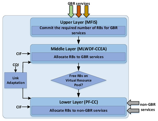
Figure 1.
The layer stack of the proposed scheme.
3.1.1. The Upper Layer of the Network Slicing Scheme
A set of GBR services per user u require resources to satisfy their constraints during the TTI. For each service, the indicator is defined, determining the estimated satisfaction grade of user u during the upcoming TTI that is the next TTI for which RBs are going to be allocated.
The value are estimated using the Mamdani Fuzzy Inference System (MFIS) system described in [27], where the and the parameters are considered as inputs expressed as Interval Valued Octagonal Fuzzy Numbers (IVOFNs) [28]. The linguistic terms and the corresponding IVOFNs used for the representation of the , the and the values are presented in Table 1. Additionally, Table 2 presents the knowledge base of the MFIS which consists of the fuzzy rules considered for the estimation of the parameter.

Table 1.
Linguistic terms and the corresponding interval-valued octagonal fuzzy numbers used for , and .
Table 2.
The Fuzzy rule (or knowledge) base.
In particular, the parameter represents the communication energy consumption. It is calculated using Equation (7) [29], where is the cell density in the area of the user and, thus, represents the number of PoAs connected to a user moving in an area with radius R. It has to be noted that in our case is assumed to be equal to 1. Additionally, is a power amplifier parameter, is the transmission power of the PoA in Watts, is the fixed power at PoA in Watts, is the local oscillator power in Watts, is the number of used antennas, is the Radio Frequency (RF) chain power [30] at the base station in Watts, is the energy per complex operation in Joules, is the available bandwidth in MHz, is the spectral efficiency of the downlink channel measured in bps/Hz, is the channel coding power measured in , is the channel decoding power measured in , and is the RF chain power at user equipment measured in Watts.
Furthermore, the parameter represents the estimated quality of the user’s service regarding the available RBs in the TTI. is calculated using Equation (8) which applies the Simple Additive Weighting (SAW) method described in [31]. In this equation, the , the , the and the parameters represent the throughput, the packet transfer delay, the jitter and the packet loss ratio parameter, respectively.
In particular, the is estimated using Equation (9), where represents the estimated throughput per RB and is the number of the RBs that are available for allocation.
Additionally, the values of the , and parameters are calculated using Equations (10)–(12), respectively. It has to be noted that, is the average packet size, is the past average packet transfer delay and is the required throughput of the service of user u. Additionally, the , , and in (8) represent the weights of the aforementioned parameters. In this work, the considered weights are calculated using the Fuzzy Analytic Network Process (FANP) method described in [27] which in this work is implemented using IVOFNs.
The minimum acceptable satisfaction grades per user and service are obtained using the and the threshold values defined in [32].
3.1.1.1. The Mamdani Satisfaction Chart
During the instantiation of the system architecture, a Mamdani satisfaction chart, which containts the values obtained for each possible and combination, is created. Specifically, each satisfaction indicator of Figure 2 is obtained using the MFIS method, considering the and the as input parameters. For simplicity purposes, both and are supposed to be normalized in order to have values within the range [0, 1], while the normalization process is described in the Section 3.1.1.2. Additionally, the , , membership functions (MF) are defined using the Equalized Universe Method (EUM) method [27], indicating the linguistic terms and the corresponding IVOFNs for the fuzzy representation of the , and factor, respectively. Thus, for each crisp value, two membership degrees are determined in the corresponding MF, one for the upper octagon and one for the lower octagon. Table 1 represents the linguistic terms and the corresponding IVOFNs of , and membership functions, which are equally distributed inside the domain [] = [0, 1], as described in [27]. Furthermore, Table 2 presents the considered fuzzy rule base which is used from the MFIS for producing the satisfaction chart.
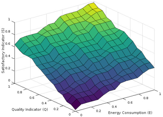
Figure 2.
The S values range as obtained using the Mamdani Fuzzy Inference System.
Indicatively, when the and values are too low, the produced value is too low as well. On the contrary, when the and values are close to 1, the produced value is also high, indicating that the user is fully satisfied. Furthermore, when only one of the or the values is close to 0, the user satisfaction is in low levels.
3.1.1.2. Performing Lookup at the Satisfaction Indicators Chart and Normalization of the Input Values
At this point it has to be noted that since the user’s satisfaction is obtained at the Fog by performing a lookup at the satisfaction indicators chart, the overhead introduced is minimal. Additionally, the method does not impose any significant overhead at the user equipment due to monitoring of the and parameters. In addition, for performing the aforementioned lookup at the chart, the values of both the and the parameters are normalized in order to be within the range [0, 1]. The normalization of the values is performed using Equations (13) and (14) for the and parameters, respectively. In these formulas, the and the parameters represent the maximum values that have been observed for the E and the Q parameters from the instantiation of the system and up to the current time point, while at the same time and .
3.1.2. The Middle Layer of the Network Slicing Scheme
In each TTI, the middle layer uses an improved version of the MLWDF-CC scheduler [23], called MLWDF with Energy Awareness (MLWDF-EA), to allocate to each GBR service the number of RBs estimated from the upper level. This scheduler extends the MLWDF-CC metric to take into consideration the estimated energy consumption of each RB. Specifically, for each ith GBR flow requiring RBs, the MLWDF-EA metric of the kth RB is estimated by Equation (15). The RB that maximizes the estimated value of the MLWDF-EA metric is allocated to the ith flow. It has to be noted that the value is determined by Equation (2). Additionally, the factor is normalized in order to obtain values inside the range (0,1]. As follows, the use of the cross carrier QoS aware MLWDF-EA scheduler realizes improved resource distribution among the GBR services. Cross carrier scheduling is deemed necessary since both the LRBs available in each PoA and the SRBs available in the Virtual Resource Pool can belong to different carriers.
3.1.3. The Lower Layer of the Network Slicing Scheme
The third layer allocates available RBs that exist to the Virtual Resource Pool to best effort flows using Equation (16) of the PF-CC [33,34] algorithm, where represents the available throughput for the ith flow in the kth RB of the t TTI and denotes the past average throughput.
3.2. The Proposed Network Architecture
The network architecture (Figure 3) includes K Points of Access (PoAs) that provide network access to the vehicular users. Each PoA () has a set of Resource Blocks (RBs), a Local Monitoring Module (LMM) and a Local Allocation Module (LAM). A variable indicates the remaining RBs of the kth PoA during the Transmission Time Interval (TTI). Additionally, the RBs of the PoA are organized into two subsets, which are called Local RBs (LRBs) and Shared RBs (SRBs).
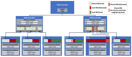
Figure 3.
The proposed Network Slicing architecture.
A set of SDN controllers manipulate the PoAs. In particular, each SDN controller maintains a Virtual Resource Pool where the SRBs of its underlying PoAs are stored. Additionally, each SDN controller includes its Allocation Module (AM). Furthermore, a centralized SDN controller with a MANO entity orchestrates the entire network slicing procedure maintaining the necessary frequency reuse factor. Specifically, during the instantiation of the system, each PoA communicates with the MANO entity to identify which subset of its RBs can be considered as SRB in order to be stored to the corresponding Virtual Resource Pool. Thus, the channel interference that can occur from the assignment of the SRBs with similar frequencies to neighbouring PoAs is minimized.
Based on the layered design of the proposed scheme the allocation of RBs to user services is as follows. Initially the LMM module of each PoA implements the Upper layer of the scheme to monitor the satisfaction grade of each user service. If the estimated is higher than the predefined threshold value, the service requirements can be satisfied from the remaining RBs that exist in the current . Thus the LAM module of the PoA implements the Middle and the Lower layers of the slicing scheme to allocate LRBs of the to both GBR and non-GBR services for the next TTI. The remaining RBs are sent back to the Virtual Resource Pool which is maintained from the corresponding SDN controller. However, if the estimated satisfaction grade is lower than the predefined threshold value, the service requirements cannot be satisfied from the . Thus, the AM of the SDN controller implements the Middle and the Lower layers of the scheme to allocate extra RBs from the Virtual Resource Pool to the user services. Regarding the Virtual Resource Pool the algorithm prefers to allocate RBs with similar sub frequencies for each user to minimize the number of antennas required for each vehicle, which is a factor that affects the energy consumption of the system.
4. Simulation Setup
In our experiments, the 5G Vehicular Cloud Computing topology presented in Figure 4 was considered. A mobility trace indicating the map of the city of Kastoria along with road traffic data was created using the Open Street Map (OSM) software [35]. Then, the mobility trace was used as input in the Simulator of Urban Mobility (SUMO) simulator [36] allowing the production of a realistic mobility pattern for the simulated vehicles including 52,843 vehicles in total, moving inside Kastoria city in a 24 h period. The average arrival rate of vehicles was equal to 0.611608796 vehicles per second, while their average departure rate was equal to 0.61025463 vehicles per second. The network topology was built upon the map, using the Network Simulator 3 (NS3) [37]. It included a Fog infrastructure, as well as a Cloud infrastructure.
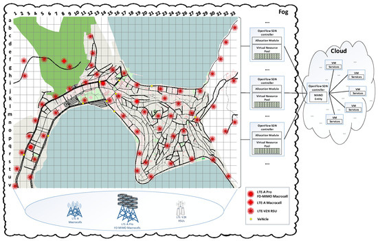
Figure 4.
The simulated topology.
The Fog infrastructure consisted of 2 LTE-A Pro FD-MIMO Macrocell evolved-NodeBs (eNBs) with 64-element antennas each, two LTE-A Macrocell eNBs with four-element antennas each and 60 LTE-V2X RSUs with four-element antennas each. The macrocells of the access networks were located on the map, according to the Hellenic Telecommunications and Post Commission (EETT) [38] data, while the LTE-V2X RSUs were added in order for the Ultra Dense Network (UDN) architecture to be further enhanced. Additionally, the Fog infrastructure included a set of OpenFlow SDN controllers. Each controller manipulated a subset of the aforementioned access networks. The functionality of each controller was extended by including a Virtual Resource Pool, a Monitoring Module (MM) and an Allocation Module (AM). The positions, the spectrum and the related SDN controller for each cell are presented in Table A1 and Table A2 (Appendix A), for the LTE Macroecell eNBs and the LTE-V2X RSUs, respectively.
The Cloud infrastructure included a set of Virtual Machines (VMs) providing services such as Conversational Voice (CVo), Conversational Video (CVi), Autonomous Navigation (ANav), Route Guidance (RG), Buffered Streaming (BS) and Web Browsing (WB). Table 3 presents the 5QI value assigned to each service, along with the corresponding constrains of each 5QI as they are defined in the 5G-PPP specifications for 5G communications [32]. Each vehicle received one flow for each service and requires RBs in each TTI to satisfy its constraints. Furthermore, an OpenFlow SDN controller provided centralized control of the entire system, while its functionality was extended with a MANO entity that orchestrated the entire functionality of the system. Table 4 presents the simulation parameters.
Table 3.
The 5QI value and the corresponding constraints for each service.
Table 4.
The simulation parameters.
During the network slicing process, the user satisfaction is obtained by a lookup to the MFIS Satisfaction Chart, using the estimated and values. It should be noted that the services’ weights used for the estimation are calculated using the FANP method [27]. The criteria used include throughput, delay, jitter and packet loss. Indicativelly, Table 5 presents the FANP pairwise comparison matrix for the ANav service, while the estimated weights for each service are depicted in Figure 5.
Table 5.
The pairwise comparison matrices for the ANav service.
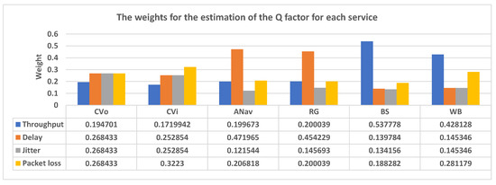
Figure 5.
The FANP weights used for the estimation of .
5. Experimental Results and Discussion
The proposed scheme is compared with the URLLC-AVN scheme described in [25], considering parameters such as the packet transfer delay, the jitter, the throughput and the packet loss ratio. In particular, Table 6 presents the average evaluation results achieved from each scheme during the 24-h simulation, indicating that the proposed scheme achieves improved system performance in all cases. Furthermore, Figure 6 presents the average packet transfer delay achieved from each scheme for every moment during the 24-h simulation. As can be observed both schemes satisfied the delay constraint defined from the 5G-PPP specifications for each service. However, the proposed scheme achieved lower delay values in all cases. Indicatively, for the CVo service slice, the packet transfer delays observed in the case of the proposed scheme were approximately 20 ms lower than the ones observed in the case of the URLLC-AVN scheme. Furthermore, in Figure 7 and Figure 8 the two schemes are compared considering the jitter and the throughput factors, respectively. Similar to the packet transfer delay results, the proposed scheme achieved better results ensuring higher service quality in all cases. In particular, the proposed scheme attained up to 10 ms lower jitter and up to 50 kbps higher throughput in some cases. Similarly, in Figure 9 the two schemes are compared considering the Packet Loss Ratio (PLR) factor, which is a very critical parameter for the considered services. As it is observed, the proposed scheme satisfied the PLR constraint for the entire services, for every moment of the simulation, while at the same time the URLLC-AVN scheme did not satisfy this constraint in any case. Thus, in cases where the URLLC-AVN scheme was used, critical information may have been lost leading to undesirable situations in some cases (e.g., road accident in case of ANav services).
Table 6.
The average evaluation results achieved from each scheme during the 24-h simulation.
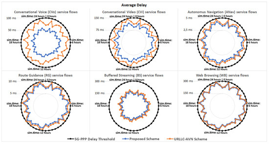
Figure 6.
The average delay observed for each service type.
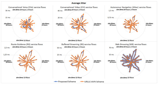
Figure 7.
The average jitter observed for each service type.
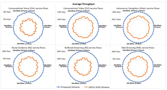
Figure 8.
The average throughput observed for each service type.
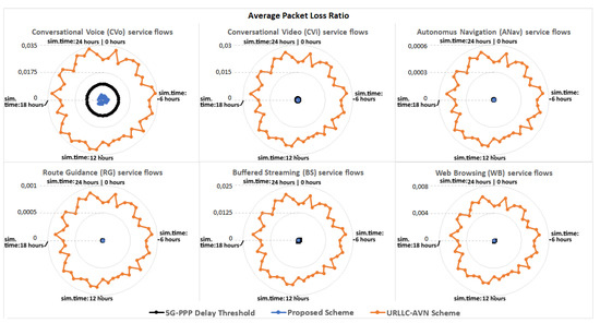
Figure 9.
The average Packet Loss Ratio observed for each service type.
Both schemes were capable of using shared communication resources to satisfy the requirements of user services. As a result, in most cases plenty of SRBs were available for allocation from each corresponding Virtual Resource Pool. Figure 10 presents the average saturation level observed in each Virtual Resource Pool during the simulation. In particular, the saturation levels in the Virtual Resource Pools maintained in SDN Controller 1 and SDN Controller 2 were low, since both controllers manipulated LTE-A Pro FD-MIMO Macrocells with plenty of resources, along with the other cells. Additionally, the rest Virtual Resource Pools obtained approximately from 45% and up to 65% average saturation. It has to be noted that in all cases the proposed scheme resulted in slightly higher saturation of communication resources in each Virtual Resource Pool, since it committed additional resources considering more parameters in comparison with the ones considered from the URLLC-AVN, including the throughput, the delay, the jitter and the packet loss ratio. On the contrary, the URLLC-AVN scheme committed additional resources considering only the delay factor. Thus, the URLLC-AVN scheme stopped the commitment of additional resources when the delay factor was satisfied. However, the satisfaction of the packet transfer delay did not impose the satisfaction of the additional parameters considered in the proposed scheme. As a result, the proposed scheme enhanced the resource allocation in all cases. Finally, both schemes were compared considering the total energy consumption observed for each scheme during the 24 h simulation. Specifically, Figure 11 shows that the proposed scheme achieved up to 100 Joules lower energy consumption during the simulation. This energy reduction can be explained since the proposed scheme took into consideration the energy consumption factor to perform the resource allocation.
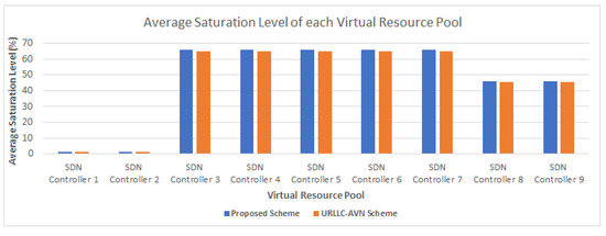
Figure 10.
The average resource saturation level observed in each Virtual Resource Pool.
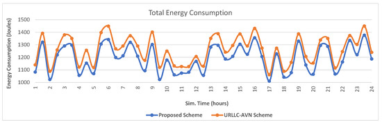
Figure 11.
The total energy consumption observed for each scheme.
6. Conclusions
In this paper a network slicing scheme for 5G-VCC systems is described. The proposed scheme improves the performance of modern vehicular services. Specifically, the QoS that each user perceives for his services as well as the energy consumption that each access network causes to user equipment are considered. Subsequently, the satisfaction grade of the user services is estimated by taking into consideration both the QoS and the energy consumption factors. If the estimated satisfaction grade is lower than a predefined threshold, additional RBs from the neighbouring PoAs are committed in order for the available resources to be increased. The orchestration of the entire procedure is performed by a MANO entity which is implemented by a centralized SDN controller. Performance evaluation showed that the proposed scheme outperforms existing solutions in terms of packet transfer delay, jitter, throughput and packet loss ratio. Future work includes the deployment of Unmanned Aerial Vehicles (UAVs) to operate as aerial relays to offload part of the RSUs tasks. Additionally, in order to further improve the proposed network slicing architecture, the design recommendations and specifications of the upcoming Sixth Generation (6G) wireless networks as well as their novel services will be studied.
Author Contributions
Conceptualization, E.S., A.M., D.J.V. and E.T.M.; investigation, E.S. and A.M.; supervision, A.M. and D.D.V.; visualization, E.S.; writing—original draft, E.S.; writing—review and editing, E.S., A.M., D.J.V., E.T.M., N.I.M. and D.D.V. All authors have read and agreed to the published version of the manuscript.
Funding
This research was partially funded by the University of Western Macedonia Research Committee.
Data Availability Statement
Simulation data can be provided after contacting the corresponding author.
Acknowledgments
This work is partly supported by the University of Western Macedonia Research Committee.
Conflicts of Interest
The authors declare no conflict of interest.
Appendix A. The Positions and the Frequencies of the Available Networks
Table A1.
The positions and the frequencies of the available LTE-A Pro FD-MIMO Macrocells.
Table A1.
The positions and the frequencies of the available LTE-A Pro FD-MIMO Macrocells.
| Network (Position) | Geographic Coordinates (Latitude, Longitude) | Number of Antennas | SDN Controller |
|---|---|---|---|
| LTE-A Pro FD-MIMO Macrocell 1 (i14) | 37.987778, 23.731667 | 64 | SDN 1 |
| LTE-A Pro FD-MIMO Macrocell 2 (q3) | 37.986389, 23.721111 | 64 | SDN 2 |
| Spectrum in MHz for each Antenna | |||
| Antenna Identifier | Downlink & Uplink Spectrum in MHz (LTE Band) | ||
| 1 | 462.5–467.5 & 452.5–457.5 (31) | ||
| 2 | 734–739 & 704–709 (17) | ||
| 3 | 739–744 & 709–714 (17) | ||
| 4 | 758–763 & 714–719 (28) | ||
| 5 | 763–768 & 719–724 (28) | ||
| 6 | 768–773 & 724–729 (28) | ||
| 7 | 773–778 & 729–734 (28) | ||
| 8 | 860–865 & 815–820 (18) | ||
| 9 | 865–870 & 820–825 (18) | ||
| 10 | 870–875 & 825–830 (18) | ||
| 11 | 875–880 & 830–835 (19) | ||
| 12 | 880–885 & 835–840 (19) | ||
| 13 | 885–890 & 840–845 (19) | ||
| 14 | 925–930 & 890–895 (8) | ||
| 15 | 930–935 & 895–900 (8) | ||
| 16 | 935–940 & 900–905 (8) | ||
| 17 | 940–945 & 905–910 (8) | ||
| 18 | 945–950 & 910–915 (8) | ||
| 19 | 1475.9–1480.9 & 1427.9–1432.9 (11) | ||
| 20 | 1480.9–1485.9 & 1432.9–1437.9 (11) | ||
| 21 | 1485.9–1490.9 & 1437.9–1442.9 (11) | ||
| 22 | 1490.9–1495.9 & 1442.9–1447.9 (11) | ||
| 23 | 1495.9–1500.9 & 1447.9–1452.9 (11) | ||
| 24 | 1525–1530 & 1625.5–1630.5 (24) | ||
| 25 | 1530–1535 & 1630.5–1635.5 (24) | ||
| 26 | 1535–1540 & 1635.5–1640.5 (24) | ||
| 27 | 1540–1545 & 1640.5–1645.5 (24) | ||
| 28 | 1545–1550 & 1645.5–1650.5 (24) | ||
| 29 | 1550–1555 & 1650.5–1655.5 (24) | ||
| 30 | 1805–1810 & 1710–1715 (3) | ||
| 31 | 1810–1815 & 1715–1720 (3) | ||
| 32 | 1815–1820 & 1720–1725 (3) | ||
| 33 | 1820–1825 & 1725–1730 (3) | ||
| 34 | 1825–1830 & 1730–1735 (3) | ||
| 35 | 1830–1835 & 1735–1740 (3) | ||
| 36 | 1835–1840 & 1740–1745 (3) | ||
| 37 | 1840–1845 & 1745–1750 (3) | ||
| 38 | 1845–1850 & 1750–1755 (3) | ||
| 39 | 1850–1855 & 1755–1760 (3) | ||
| 40 | 1855–1860 & 1760–1765 (3) | ||
| 41 | 1860–1865 & 1765–1770 (3) | ||
| 42 | 1865–1870 & 1770–1775 (3) | ||
| 43 | 1870–1875 & 1775–1780 (3) | ||
| 44 | 1875–1880 & 1780–1785 (3) | ||
| 45 | 1930–1935 & 1880–1885 (2) | ||
| 46 | 1935–1940 & 1885–1890 (2) | ||
| 47 | 1940–1945 & 1890–1895 (2) | ||
| 48 | 1945–1950 & 1895–1900 (2) | ||
| 49 | 1950–1955 & 1900–1905 (2) | ||
| 50 | 1955–1960 & 1905–1910 (2) | ||
| 51 | 2600–2605 & 1910–1915 (15) | ||
| 52 | 2605–2610 & 1915–1920 (15) | ||
| 53 | 2110–2115 & 1960–1965 (1) | ||
| 54 | 2115–2120 & 1965–1970 (1) | ||
| 55 | 2120–2125 & 1970–1975 (1) | ||
| 56 | 2125–2130 & 1975–1980 (1) | ||
| 57 | 2180–2185 & 2000–2005 (23) | ||
| 58 | 2185–2190 & 2005–2010 (23) | ||
| 59 | 2190–2195 & 2010–2015 (23) | ||
| 60 | 2195–2200 & 2015–2020 (23) | ||
| 61 | 2595–2600 & 2020–2025 (16) | ||
| 62 | 2350–2355 & 2305–2310 (30) | ||
| 63 | 2355–2360 & 2310–2315 (30) | ||
| 64 | 2620–2625 & 2500–2505 (7) | ||
Table A2.
The positions and the frequencies of the available LTE–A Macrocells and LTE V2X RSUs.
Table A2.
The positions and the frequencies of the available LTE–A Macrocells and LTE V2X RSUs.
| Network (Position) | Geographic Coordinates (Latitude, Longitude) | Downlink Spectrum in MHz: Antenna 1, Antenna 2, Antenna 3, Antenna 4 (LTE Band) | Uplink Spectrum in MHz: Antenna 1, Antenna 2, Antenna 3, Antenna 4 (LTE Band) | SDN Controller |
|---|---|---|---|---|
| LTE Macro 1 (f8) | 40.524167, 21.258056 | 2625–2630, 2630–2635, 2635–2640, 2640–2645 (7) | 2505–2510, 2510–2515, 2515–2520, 2520–2525 (7) | SDN 8 |
| LTE Macro 2 (k19) | 40.524167, 21.270556 | 2645–2650, 2650–2655, 2655–2660, 2660–2665 (7) | 2525–2530, 2530–2535, 2535–2540, 2520–2545 (7) | SDN 9 |
| LTE–V2X 1 (b33) | 40.527296, 21.277442 | 3510–3512.5, 3512.5–3515, 3515–3517.5, 3517.5–3520 (22) | 3410–3412.5, 3412.5–3415, 3415–3417.5, 3417.5–3420 (22) | SDN 1 |
| LTE–V2X 2 (c12) | 40.526583, 21.260826 | 3550–3552.5, 3552.5–3555, 3555–3557.5, 3557.5–3560 (22) | 3450–3452.5, 3452.5–3455, 3455–3457.5, 3457.5–3460 (22) | SDN 1 |
| LTE–V2X 3 (d32) | 40.526032, 21.276358 | 3520–3522.5, 3522.5–3525, 3525–3527.5, 3527.5–3530 (22) | 3420–3422.5, 3422.5–3425, 3425–3427.5, 3427.5–3430 (22) | SDN 2 |
| LTE–V2X 4 (e12) | 40.524819, 21.261104 | 3590–3592.5, 3592.5–3595, 3595–3597.5, 3597.5–3600 (22) | 3490–3492.5, 3492.5–3495, 3495–3497.5, 3497.5–3500 (22) | SDN 1 |
| LTE–V2X 5 (f2) | 40.523786, 21.253099 | 3520–3522.5, 3522.5–3525, 3525–3527.5, 3527.5–3530 (22) | 3420–3422.5, 3422.5–3425, 3425–3427.5, 3427.5–3430 (22) | SDN 3 |
| LTE–V2X 6 (f31) | 40.524646, 21.275628 | 3550–3552.5, 3552.5–3555, 3555–3557.5, 3557.5–3560 (22) | 3450–3452.5, 3452.5–3455, 3455–3457.5, 3457.5–3460 (22) | SDN 2 |
| LTE–V2X 7 (f5) | 40.524328, 21.255603 | 3510–3512.5, 3512.5–3515, 3515–3517.5, 3517.5–3520 (22) | 3410–3412.5, 3412.5–3415, 3415–3417.5, 3417.5–3420 (22) | SDN 2 |
| LTE–V2X 8 (g12) | 40.523696, 21.260837 | 3540–3542.5, 3542.5–3545, 3545–3547.5, 3547.5–3550 (22) | 3440–3442.5, 3442.5–3445, 3445–3447.5, 3447.5–3450 (22) | SDN 2 |
| LTE–V2X 9 (g15) | 40.523305, 21.263379 | 3550–3552.5, 3552.5–3555, 3555–3557.5, 3557.5–3560 (22) | 3450–3452.5, 3452.5–3455, 3455–3457.5, 3457.5–3460 (22) | SDN 3 |
| LTE–V2X 10 (g9) | 40.523692, 21.258844 | 3570–3572.5, 3572.5–3575, 3575–3577.5, 3577.5–3580 (22) | 3470–3472.5, 3472.5–3475, 3475–3477.5, 3477.5–3480 (22) | SDN 1 |
| LTE–V2X 11 (h13) | 40.522762, 21.261590 | 3530–3532.5, 3532.5–3535, 3535–3537.5, 3537.5–3540 (22) | 3430–3432.5, 3432.5–3435, 3435–3437.5, 3437.5–3440 (22) | SDN 1 |
| LTE–V2X 12 (h17) | 40.522889, 21.264763 | 3510–3512.5, 3512.5–3515, 3515–3517.5, 3517.5–3520 (22) | 3410–3412.5, 3412.5–3415, 3415–3417.5, 3417.5–3420 (22) | SDN 3 |
| LTE–V2X 13 (h2) | 40.522746, 21.252932 | 3530–3532.5, 3532.5–3535, 3535–3537.5, 3537.5–3540 (22) | 3430–3432.5, 3432.5–3435, 3435–3437.5, 3437.5–3440 (22) | SDN 3 |
| LTE–V2X 14 (h30) | 40.523113, 21.274598 | 3540–3542.5, 3542.5–3545, 3545–3547.5, 3547.5–3550 (22) | 3440–3442.5, 3442.5–3445, 3445–3447.5, 3447.5–3450 (22) | SDN 3 |
| LTE–V2X 15 (i11) | 40.522163, 21.260125 | 3560–3562.5, 3562.5–3565, 3565–3567.5, 3567.5–3570 (22) | 3460–3462.5, 3462.5–3465, 3465–3467.5, 3467.5–3470 (22) | SDN 4 |
| LTE–V2X 16 (i19) | 40.522016, 21.266329 | 3520–3522.5, 3522.5–3525, 3525–3527.5, 3527.5–3530 (22) | 3420–3422.5, 3422.5–3425, 3425–3427.5, 3427.5–3430 (22) | SDN 4 |
| LTE–V2X 17 (i33) | 40.522453, 21.277232 | 3510–3512.5, 3512.5–3515, 3515–3517.5, 3517.5–3520 (22) | 3410–3412.5, 3412.5–3415, 3415–3417.5, 3417.5–3420 (22) | SDN 4 |
| LTE–V2X 18 (j22) | 40.521787, 21.268839 | 3550–3552.5, 3552.5–3555, 3555–3557.5, 3557.5–3560 (22) | 3450–3452.5, 3452.5–3455, 3455–3457.5, 3457.5–3460 (22) | SDN 4 |
| LTE–V2X 19 (j25) | 40.521608, 21.271178 | 3530–3532.5, 3532.5–3535, 3535–3537.5, 3537.5–3540 (22) | 3430–3432.5, 3432.5–3435, 3435–3437.5, 3437.5–3440 (22) | SDN 4 |
| LTE–V2X 20 (j28) | 40.521594, 21.273391 | 3560–3562.5, 3562.5–3565, 3565–3567.5, 3567.5–3570 (22) | 3460–3462.5, 3462.5–3465, 3465–3467.5, 3467.5–3470 (22) | SDN 5 |
| LTE–V2X 21 (j9) | 40.521637, 21.258371 | 3550–3552.5, 3552.5–3555, 3555–3557.5, 3557.5–3560 (22) | 3450–3452.5, 3452.5–3455, 3455–3457.5, 3457.5–3460 (22) | SDN 5 |
| LTE–V2X 22 (k11) | 40.520579, 21.260202 | 3590–3592.5, 3592.5–3595, 3595–3597.5, 3597.5–3600 (22) | 3490–3492.5, 3492.5–3495, 3495–3497.5, 3497.5–3500 (22) | SDN 2 |
| LTE–V2X 23 (k15) | 40.520582, 21.262836 | 3570–3572.5, 3572.5–3575, 3575–3577.5, 3577.5–3580 (22) | 3470–3472.5, 3472.5–3475, 3475–3477.5, 3477.5–3480 (22) | SDN 2 |
| LTE–V2X 24 (k16) | 40.520959, 21.264330 | 3580–3582.5, 3582.5–3585, 3585–3587.5, 3587.5–3590 (22) | 3480–3482.5, 3482.5–3485, 3485–3487.5, 3487.5–3490 (22) | SDN 1 |
| LTE–V2X 25 (k23) | 40.520580, 21.269367 | 3590–3592.5, 3592.5–3595, 3595–3597.5, 3597.5–3600 (22) | 3490–3492.5, 3492.5–3495, 3495–3497.5, 3497.5–3500 (22) | SDN 3 |
| LTE–V2X 26 (k7) | 40.520940, 21.256585 | 3540–3542.5, 3542.5–3545, 3545–3547.5, 3547.5–3550 (22) | 3440–3442.5, 3442.5–3445, 3445–3447.5, 3447.5–3450 (22) | SDN 4 |
| LTE–V2X 27 (l25) | 40.520507, 21.270952 | 3510–3512.5, 3512.5–3515, 3515–3517.5, 3517.5–3520 (22) | 3410–3412.5, 3412.5–3415, 3415–3417.5, 3417.5–3420 (22) | SDN 5 |
| LTE–V2X 28 (l30) | 40.520212, 21.274900 | 3570–3572.5, 3572.5–3575, 3575–3577.5, 3577.5–3580 (22) | 3470–3472.5, 3472.5–3475, 3475–3477.5, 3477.5–3480 (22) | SDN 3 |
| LTE–V2X 29 (l5) | 40.520316, 21.255158 | 3510–3512.5, 3512.5–3515, 3515–3517.5, 3517.5–3520 (22) | 3410–3412.5, 3412.5–3415, 3415–3417.5, 3417.5–3420 (22) | SDN 6 |
| LTE–V2X 30 (m17) | 40.519163, 21.264467 | 3520–3522.5, 3522.5–3525, 3525–3527.5, 3527.5–3530 (22) | 3420–3422.5, 3422.5–3425, 3425–3427.5, 3427.5–3430 (22) | SDN 5 |
| LTE–V2X 31 (m20) | 40.519652, 21.267214 | 3540–3542.5, 3542.5–3545, 3545–3547.5, 3547.5–3550 (22) | 3440–3442.5, 3442.5–3445, 3445–3447.5, 3447.5–3450 (22) | SDN 5 |
| LTE–V2X 32 (m22) | 40.519205, 21.268504 | 3560–3562.5, 3562.5–3565, 3565–3567.5, 3567.5–3570 (22) | 3460–3462.5, 3462.5–3465, 3465–3467.5, 3467.5–3470 (22) | SDN 6 |
| LTE–V2X 33 (m24) | 40.519181, 21.270182 | 3520–3522.5, 3522.5–3525, 3525–3527.5, 3527.5–3530 (22) | 3420–3422.5, 3422.5–3425, 3425–3427.5, 3427.5–3430 (22) | SDN 6 |
| LTE–V2X 34 (m27) | 40.519431, 21.272556 | 3590–3592.5 3592.5–3595, 3595–3597.5, 3597.5–3600 (22) | 3490–3492.5, 3492.5–3495, 3495–3497.5, 3497.5–3500 (22) | SDN 4 |
| LTE–V2X 35 (m7) | 40.519535, 21.256973 | 3520–3522.5, 3522.5–3525, 3525–3527.5, 3527.5–3530 (22) | 3420–3422.5, 3422.5–3425, 3425–3427.5, 3427.5–3430 (22) | SDN 7 |
| LTE–V2X 36 (n28) | 40.518833, 21.273332 | 3540–3542.5, 3542.5–3545, 3545–3547.5, 3547.5–3550 (22) | 3440–3442.5, 3442.5–3445, 3445–3447.5, 3447.5–3450 (22) | SDN 6 |
| LTE–V2X 37 (n33) | 40.518765, 21.277286 | 3580–3582.5, 3582.5–3585, 3585–3587.5, 3587.5–3590 (22) | 3480–3482.5, 3482.5–3485, 3485–3487.5, 3487.5–3490 (22) | SDN 2 |
| LTE–V2X 38 (n4) | 40.518893, 21.254445 | 3580–3582.5, 3582.5–3585, 3585–3587.5, 3587.5–3590 (22) | 3480–3482.5, 3482.5–3485, 3485–3487.5, 3487.5–3490 (22) | SDN 8 |
| LTE–V2X 39 (o19) | 40.517749, 21.266052 | 3590–3592.5, 3592.5–3595, 3595–3597.5, 3597.5–3600 (22) | 3490–3492.5, 3492.5–3495, 3495–3497.5, 3497.5–3500 (22) | SDN 5 |
| LTE–V2X 40 (o22) | 40.517920 21.268739 | 3530–3532.5, 3532.5–3535, 3535–3537.5, 3537.5–3540 (22) | 3430–3432.5, 3432.5–3435, 3435–3437.5, 3437.5–3440 (22) | SDN 5 |
| LTE–V2X 41 (o26) | 40.517917, 21.271664 | 3550–3552.5, 3552.5–3555, 3555–3557.5, 3557.5–3560 (22) | 3450–3452.5, 3452.5–3455, 3455–3457.5, 3457.5–3460 (22) | SDN 6 |
| LTE–V2X 42 (o32) | 40.517755, 21.276493 | 3530–3532.5, 3532.5–3535, 3535–3537.5, 3537.5–3540 (22) | 3430–3432.5, 3432.5–3435, 3435–3437.5, 3437.5–3440 (22) | SDN 6 |
| LTE–V2X 43 (p24) | 40.517455, 21.270338 | 3570–3572.5, 3572.5–3575, 3575–3577.5, 3577.5–3580 (22) | 3470–3472.5, 3472.5–3475, 3475–3477.5, 3477.5–3480 (22) | SDN 6 |
| LTE–V2X 44 (p3) | 40.517490, 21.253748 | 3560–3562.5, 3562.5–3565, 3565–3567.5, 3567.5–3570 (22) | 3460–3462.5, 3462.5–3465, 3465–3467.5, 3467.5–3470 (22) | SDN 7 |
| LTE–V2X 45 (p30) | 40.517055, 21.274813 | 3560–3562.5, 3562.5–3565, 3565–3567.5, 3567.5–3570 (22) | 3460–3462.5, 3462.5–3465, 3465–3467.5, 3467.5–3470 (22) | SDN 8 |
| LTE–V2X 46 (p5) | 40.517527, 21.255565 | 3570–3572.5, 3572.5–3575, 3575–3577.5, 3577.5–3580 (22) | 3470–3472.5, 3472.5–3475, 3475–3477.5, 3477.5–3480 (22) | SDN 7 |
| LTE–V2X 47 (q23) | 40.516694, 21.269523 | 3510–3512.5, 3512.5–3515, 3515–3517.5, 3517.5–3520 (22) | 3410–3412.5, 3412.5–3415, 3415–3417.5, 3417.5–3420 (22) | SDN 7 |
| LTE–V2X 48 (r19) | 40.515949, 21.266270 | 3570–3572.5, 3572.5–3575, 3575–3577.5, 3577.5–3580 (22) | 3470–3472.5, 3472.5–3475, 3475–3477.5, 3477.5–3480 (22) | SDN 8 |
| LTE–V2X 49 (r2) | 40.515521, 21.252794 | 3550–3552.5, 3552.5–3555, 3555–3557.5, 3557.5–3560 (22) | 3450–3452.5, 3452.5–3455, 3455–3457.5, 3457.5–3460 (22) | SDN 7 |
| LTE–V2X 50 (s20) | 40.515218, 21.267110 | 3520–3522.5, 3522.5–3525, 3525–3527.5, 3527.5–3530 (22) | 3420–3422.5, 3422.5–3425, 3425–3427.5, 3427.5–3430 (22) | SDN 8 |
| LTE–V2X 51 (s24) | 40.515186, 21.270210 | 3580–3582.5, 3582.5–3585, 3585–3587.5, 3587.5–3590 (22) | 3480–3482.5, 3482.5–3485, 3485–3487.5, 3487.5–3490 (22) | SDN 9 |
| LTE–V2X 52 (s27) | 40.515476, 21.272431 | 3570–3572.5, 3572.5–3575, 3575–3577.5, 3577.5–3580 (22) | 3470–3472.5, 3472.5–3475, 3475–3477.5, 3477.5–3480 (22) | SDN 9 |
| LTE–V2X 53 (s30) | 40.515406, 21.274918 | 3540–3542.5, 3542.5–3545, 3545–3547.5, 3547.5–3550 (22) | 3440–3442.5, 3442.5–3445, 3445–3447.5, 3447.5–3450 (22) | SDN 7 |
| LTE–V2X 54 (s4) | 40.515366, 21.254417 | 3540–3542.5, 3542.5–3545, 3545–3547.5, 3547.5–3550 (22) | 3440–3442.5, 3442.5–3445, 3445–3447.5, 3447.5–3450 (22) | SDN 8 |
| LTE–V2X 55 (t1) | 40.514812, 21.252504 | 3530–3532.5, 3532.5–3535, 3535–3537.5, 3537.5–3540 (22) | 3430–3432.5, 3432.5–3435, 3435–3437.5, 3437.5–3440 (22) | SDN 7 |
| LTE–V2X 56 (t19) | 40.514485, 21.266007 | 3540–3542.5, 3542.5–3545, 3545–3547.5, 3547.5–3550 (22) | 3440–3442.5, 3442.5–3445, 3445–3447.5, 3447.5–3450 (22) | SDN 9 |
| LTE–V2X 57 (u21) | 40.513975, 21.267817 | 3560–3562.5, 3562.5–3565, 3565–3567.5, 3567.5–3570 (22) | 3460–3462.5, 3462.5–3465, 3465–3467.5, 3467.5–3470 (22) | SDN 9 |
| LTE–V2X 58 (u3) | 40.514014, 21.253712 | 3520–3522.5, 3522.5–3525, 3525–3527.5, 3527.5–3530 (22) | 3420–3422.5, 3422.5–3425, 3425–3427.5, 3427.5–3430 (22) | SDN 9 |
| LTE–V2X 59 (u32) | 40.513154, 21.277329 | 3510–3512.5, 3512.5–3515, 3515–3517.5, 3517.5–3520 (22) | 3410–3412.5, 3412.5–3415, 3415–3417.5, 3417.5–3420 (22) | SDN 8 |
| LTE–V2X 60 (v1) | 40.512886, 21.252198 | 3510–3512.5, 3512.5–3515, 3515–3517.5, 3517.5–3520 (22) | 3410–3412.5, 3412.5–3415, 3415–3417.5, 3417.5–3420 (22) | SDN 9 |
References
- Kazemifard, N.; Shah-Mansouri, V. Minimum delay function placement and resource allocation for Open RAN (O-RAN) 5G networks. Comput. Netw. 2021, 188, 107809. [Google Scholar] [CrossRef]
- Salhab, N.; Langar, R.; Rahim, R. 5G network slices resource orchestration using Machine Learning techniques. Comput. Netw. 2021, 188, 107829. [Google Scholar] [CrossRef]
- TR 21.915 (V15.0.0): Digital Cellular Telecommunications System (Phase 2+) (GSM); Universal Mobile Telecommunications System (UMTS); LTE; 5G; (Rel.15); Technical Specifications; 3GPP: Sophia Antipolis, France, 2019; Volume 1, pp. 1–68.
- Vaghefi, R.M.; Palat, R.C.; Marzin, G.; Basavaraju, K.; Feng, Y.; Banu, M. Achieving Phase Coherency and Gain Stability in Active Antenna Arrays for Sub-6 GHz FDD and TDD FD-MIMO: Challenges and Solutions. IEEE Access 2020, 8, 152680–152696. [Google Scholar] [CrossRef]
- Afolalu, O.; Ventura, N. Carrier aggregation-enabled non-orthogonal multiple access approach towards enhanced network performance in 5G Ultra-Dense Networks. Int. J. Commun. Syst. 2021, 34, e4701. [Google Scholar] [CrossRef]
- Neto, E.P.; Silva, F.S.D.; Schneider, L.M.; Neto, A.V.; Immich, R. Seamless MANO of multi-vendor SDN controllers across federated multi-domains. Comput. Netw. 2021, 186, 107752. [Google Scholar] [CrossRef]
- Navarro-Ortiz, J.; Romero-Diaz, P.; Sendra, S.; Ameigeiras, P.; Ramos-Munoz, J.J.; Lopez-Soler, J.M. A survey on 5G usage scenarios and traffic models. IEEE Commun. Surv. Tutor. 2020, 22, 905–929. [Google Scholar] [CrossRef]
- Arteaga, C.H.T.; Ordoñez, A.; Rendon, O.M.C. Scalability and Performance Analysis in 5G Core Network Slicing. IEEE Access 2020, 8, 142086–142100. [Google Scholar] [CrossRef]
- Marinova, S.; Lin, T.; Bannazadeh, H.; Leon-Garcia, A. End-to-end network slicing for future wireless in multi-region cloud platforms. Comput. Netw. 2020, 177, 107298. [Google Scholar] [CrossRef]
- Foukas, X.; Patounas, G.; Elmokashfi, A.; Marina, M.K. Network slicing in 5G: Survey and challenges. IEEE Commun. Mag. 2017, 55, 94–100. [Google Scholar] [CrossRef]
- Joung, J. Random space–time line code with proportional fairness scheduling. IEEE Access 2020, 8, 35253–35262. [Google Scholar] [CrossRef]
- Liu, S.; Wang, Z.; Hu, J.; Wei, G. Protocol-based extended Kalman filtering with quantization effects: The Round-Robin case. Int. J. Robust Nonlinear Control 2020, 30, 7927–7946. [Google Scholar] [CrossRef]
- Marwat, S.N.K.; Shuaib, M.; Ahmed, S.; Hafeez, A.; Tufail, M. Medium Access-Based Scheduling Scheme for Cyber Physical Systems in 5G Networks. Electronics 2020, 9, 639. [Google Scholar] [CrossRef]
- Karimi, A.; Pedersen, K.I.; Mahmood, N.H.; Pocovi, G.; Mogensen, P. Efficient low complexity packet scheduling algorithm for mixed URLLC and eMBB traffic in 5G. In Proceedings of the 2019 IEEE 89th Vehicular Technology Conference (VTC2019-Spring), Kuala Lumpur, Malaysia, 28 April–1 May 2019; pp. 1–6. [Google Scholar]
- Nojima, D.; Katsumata, Y.; Shimojo, T.; Morihiro, Y.; Asai, T.; Yamada, A.; Iwashina, S. Resource isolation in RAN part while utilizing ordinary scheduling algorithm for network slicing. In Proceedings of the 2018 IEEE 87th Vehicular Technology Conference (VTC Spring), Porto, Portugal, 3–6 June 2018; pp. 1–5. [Google Scholar]
- Bektas, C.; Bocker, S.; Kurtz, F.; Wietfeld, C. Reliable Software-Defined RAN Network Slicing for Mission-Critical 5G Communication Networks. In Proceedings of the 2019 IEEE Globecom Workshops (GC Wkshps), Waikoloa, HI, USA, 9–13 December 2019; pp. 1–6. [Google Scholar]
- Chayon, H.R.; Dimyati, K.; Ramiah, H.; Reza, A.W. An improved radio resource management with carrier aggregation in LTE advanced. Appl. Sci. 2017, 7, 394. [Google Scholar] [CrossRef]
- Chayon, H.R.; Dimyati, K.; Ramiah, H. An efficient packet scheduling algorithm to improve the performance of cell-edge user in lte network. In Proceedings of the 2017 IEEE 13th Malaysia International Conference on Communications (MICC), Johor Bahru, Malaysia, 28–30 November 2017; pp. 130–135. [Google Scholar]
- Schmidt, R.; Chang, C.Y.; Nikaein, N. Slice scheduling with QoS-guarantee towards 5G. In Proceedings of the 2019 IEEE Global Communications Conference (GLOBECOM), Waikoloa, HI, USA, 9–13 December 2019; pp. 1–7. [Google Scholar]
- Piro, G.; Grieco, L.A.; Boggia, G.; Fortuna, R.; Camarda, P. Two-level downlink scheduling for real-time multimedia services in LTE networks. IEEE Trans. Multimed. 2011, 13, 1052–1065. [Google Scholar] [CrossRef]
- Ouaissa, M.; Rhattoy, A.; Lahmer, M. Comparative performance study of QoS downlink scheduling algorithms in LTE system for M2M communications. In International Conference Europe Middle East & North Africa Information Systems and Technologies to Support Learning; Springer: Cham, Switzerland, 2018; pp. 216–224. [Google Scholar]
- Skondras, E.; Michalas, A.; Sgora, A.; Vergados, D.D. A downlink scheduler supporting real time services in LTE cellular networks. In Proceedings of the 2015 6th International Conference on Information, Intelligence, Systems and Applications (IISA), Corfu, Greece, 6–8 July 2015; pp. 1–6. [Google Scholar]
- Skondras, E.; Michalas, A.; Sgora, A.; Vergados, D.D. QoS-aware scheduling in LTE-A networks with SDN control. In Proceedings of the 2016 7th International Conference on Information, Intelligence, Systems & Applications (IISA), Chalkidiki, Greece, 13–15 July 2016; pp. 1–6. [Google Scholar]
- Shakir, S.S.H.; Rajesh, A. Performance analysis of two level calendar disc scheduling in LTE advanced system with carrier aggregation. Wirel. Pers. Commun. 2017, 95, 2855–2871. [Google Scholar] [CrossRef]
- Ge, X. Ultra-reliable low-latency communications in autonomous vehicular networks. IEEE Trans. Veh. Technol. 2019, 68, 5005–5016. [Google Scholar] [CrossRef]
- Ahmadi, M.H.E.; Royaee, S.J.; Tayyebi, S.; Boozarjomehry, R.B. A new insight into implementing Mamdani fuzzy inference system for dynamic process modeling: Application on flash separator fuzzy dynamic modeling. Eng. Appl. Artif. Intell. 2020, 90, 103485. [Google Scholar] [CrossRef]
- Skondras, E.; Michalas, A.; Vergados, D.D. Mobility management on 5g vehicular cloud computing systems. Veh. Commun. 2019, 16, 15–44. [Google Scholar] [CrossRef]
- D Dinagar, S.; Rameshan, N. Solving Critical Path in Project Scheduling by using TOPSIS Ranking of Generalized Interval Valued Octagonal Fuzzy Numbers. J. Phys. Sci. 2019, 24, 53–61. [Google Scholar]
- Mukherjee, S.; Lee, J. Edge computing-enabled cell-free massive MIMO systems. IEEE Trans. Wirel. Commun. 2020, 19, 2884–2899. [Google Scholar] [CrossRef]
- Guruprasad, R.; Son, K.; Dey, S. Power-efficient base station operation through user QoS-aware adaptive RF chain switching technique. In Proceedings of the 2015 IEEE International Conference on Communications (ICC), London, UK, 8–12 June 2015; pp. 244–250. [Google Scholar]
- Proag, V. Multi Objective Evaluation Criteria for Infrastructure. In Infrastructure Planning and Management: An Integrated Approach; Springer: Berlin/Heidelberg, Germany, 2021; pp. 411–440. [Google Scholar]
- View on 5G Architecture; Version 3; 5G PPP Architecture Working Group: Heidelberg, Germany, 2019; Volume 1, pp. 1–166.
- Mohammed Abdul Jawad, M. Al-Shibly, M.H.H.; Islam, M.R. Radio resource scheduling in LTE-Advanced system with Carrier Aggregation. ARPN J. Eng. Appl. Sci. 2015, 10, 17281–17285. [Google Scholar]
- Oh, S.; Na, J.; Kwon, D. Performance Analysis of Cross Component Carrier Scheduling in LTE Small Cell Access Point System. In Proceedings of the Second International Conference on Electrical, Electronics, Computer Engineering and their Applications (EECEA2015), Manila, Philippines, 28 January 2015; p. 146. [Google Scholar]
- Open Street Map (OSM). Available online: https://www.openstreetmap.org (accessed on 15 April 2021).
- Behrisch, M.; Bieker, L.; Erdmann, J.; Krajzewicz, D. SUMO–simulation of urban mobility: An overview. In Proceedings of the SIMUL 2011, the Third International Conference on Advances in System Simulation, ThinkMind, Barcelona, Spain, 23–29 October 2011. [Google Scholar]
- Network Simulator 3 (NS3). Available online: https://www.nsnam.org/ (accessed on 15 April 2021).
- Hellenic Telecommunications and Post Commission (EETT). 2021. Available online: http://keraies.eett.gr/ (accessed on 15 April 2021).
- NS3 OnOffApplication Class Reference. 2021. Available online: https://www.nsnam.org/doxygen/classns3_1_1_on_off_application.html (accessed on 15 April 2021).
- Skype Requirements for Video Calling. 2021. Available online: https://support.skype.com/en/faq/fa1417/how-much-bandwidth-does-skype-need (accessed on 15 April 2021).
- NS3 UdpTraceClient Class Reference. 2021. Available online: https://www.nsnam.org/doxygen/structns3_1_1_udp_trace_client.html (accessed on 15 April 2021).
- 3GPP HTTP Applications, NS3. 2021. Available online: https://www.nsnam.org/docs/models/html/applications.html (accessed on 15 April 2021).
Publisher’s Note: MDPI stays neutral with regard to jurisdictional claims in published maps and institutional affiliations. |
© 2021 by the authors. Licensee MDPI, Basel, Switzerland. This article is an open access article distributed under the terms and conditions of the Creative Commons Attribution (CC BY) license (https://creativecommons.org/licenses/by/4.0/).