
A Deep Learning-Based Classification Scheme for False Data Injection Attack Detection in Power System


Abstract
1. Introduction
- The standard DBN is improved to deal with the continuous real-time series data of the power system flexibly and extract the time correlation.
- A CDBN-based FDIA detection scheme is proposed to evaluate the reliability of the measurement and ensure the safe and stable operation of the power grid.
- By simulating different attack scenarios, the performance of the proposed scheme is evaluated from multiple aspects to ensure its feasibility and effectiveness.
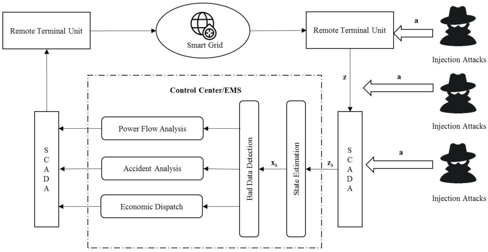
2. System Model
2.1. State Estimation in Power Systems
2.2. Conventional Bad Data Detection
3. False Data Injection Attack
- Least-effort attack [19]: k = 1, adversaries manipulate the minimum number of measurements to launch the FDIA;
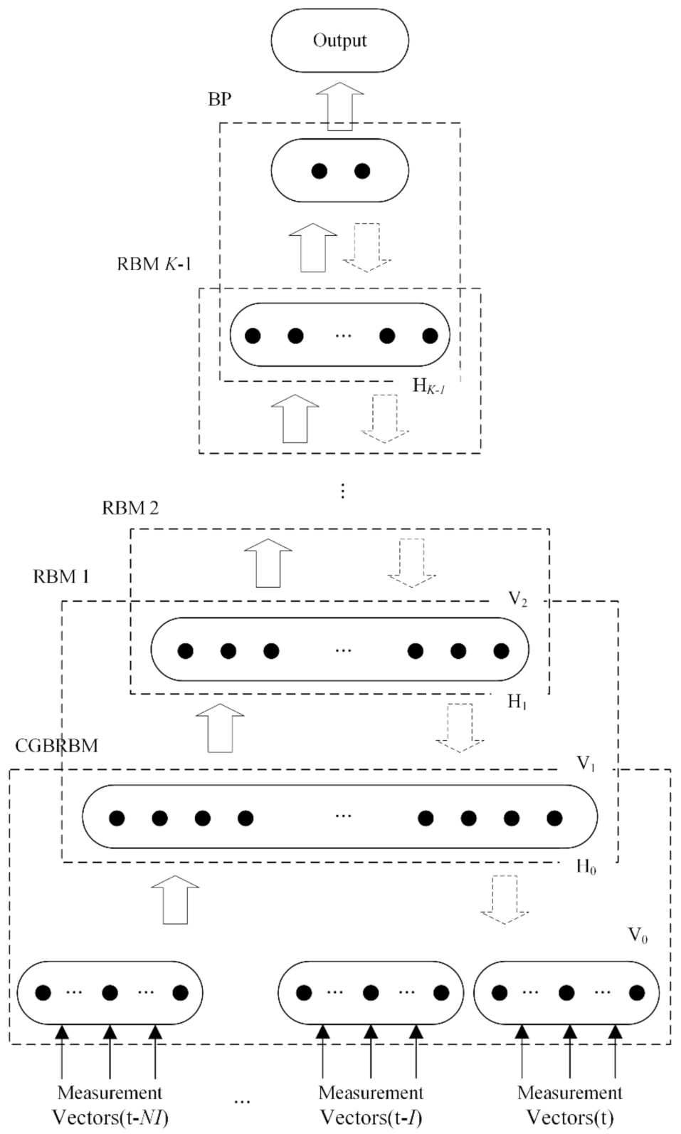
4. Deep Learning-Based Identification Scheme
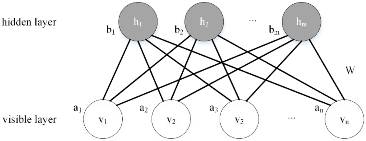
4.1. Conventional RBM
4.2. Conditional Gaussian-Bernoulli RBM
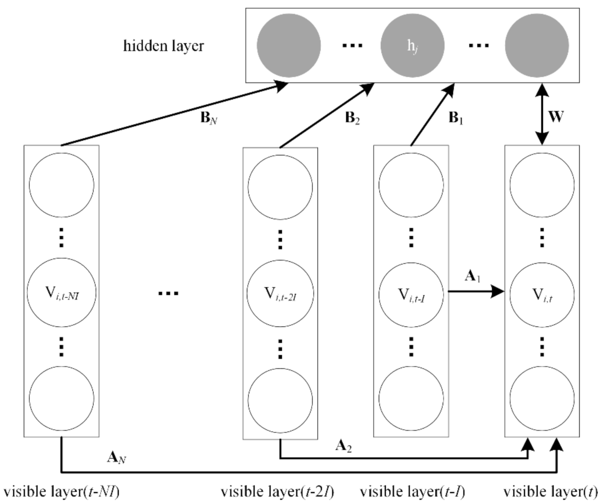
4.3. CDBN
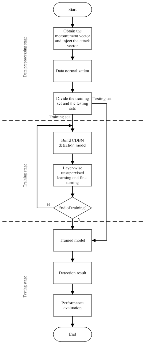
5. Simulation
5.1. Experimental Results
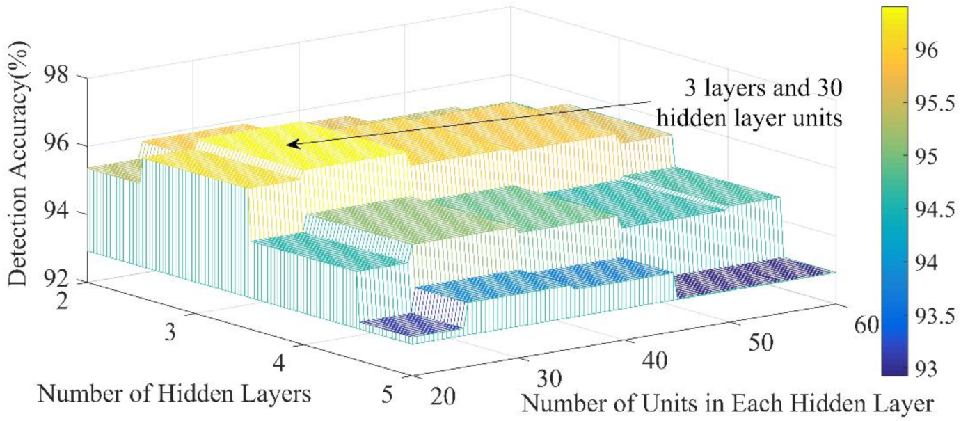
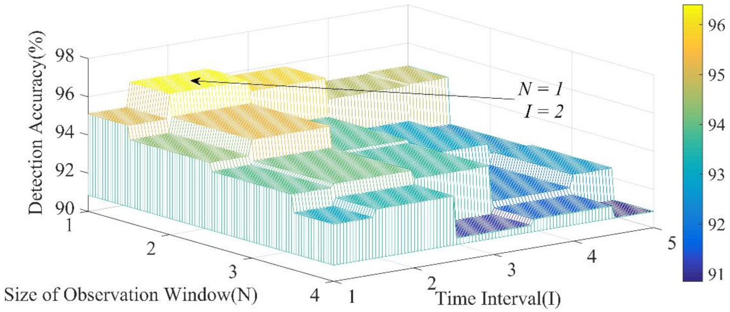
5.1.1. Structural Design
- I.
- Effect of the height and width of the CDBN
- II.
- Effect of the Observation Window Structure
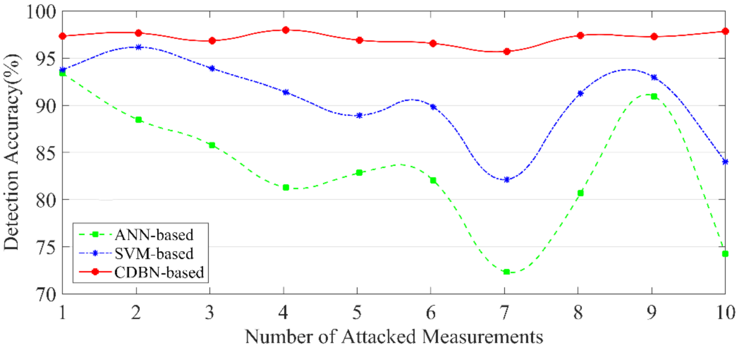
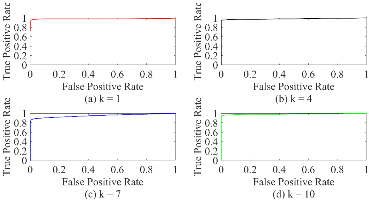
5.1.2. Multi-Scenario Validation
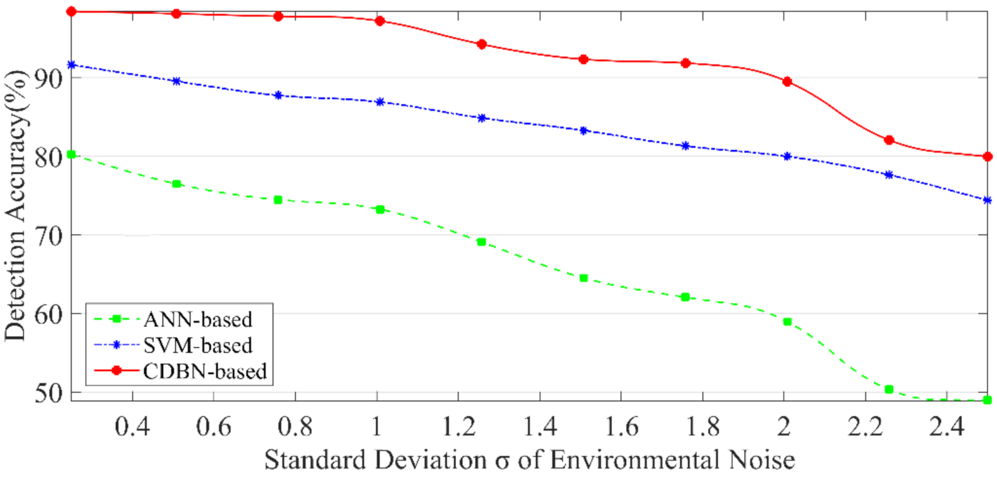
5.1.3. Robustness Validation
5.2. Analysis of Results
- The choice of the parameters
- The presence of environmental noise
- Insufficient data
6. Conclusions
Author Contributions
Funding
Data Availability Statement
Acknowledgments
Conflicts of Interest
Nomenclature
| ANN | Artificial neural network |
| AUC | Area under curve |
| BDD | Bad data detection |
| CDBN | Conditional deep belief network |
| CGBRBM | Conditional Gaussian-Bernoulli RBM |
| CD | Contrast divergence |
| DOID | Distributed observable island detection |
| DTAD | Distributed time approaching detection |
| DBN | Deep belief network |
| FDIA | False data injection attack |
| RBM | Restricted boltzmann machine |
| ROC | Receiver operating characteristics |
| SVM | Support vector machine |
| SCADA | Supervisory control and data acquisition system |
| Attack vector | |
| , | Standard biases |
| Dynamic biases from the past to the visible bias vector | |
| Weight matrices of the kth previous visible vector to the current visible unit | |
| Elements of | |
| Weight matrices of the kth previous visible vector to the current hidden unit | |
| Elements of | |
| Dynamic biases from the past to the hidden bias vector | |
| Arbitrary vector added to the state variable | |
| Measurement error vector | |
| Jacobian matrix | |
| H | Number of elements in each layer of CDBN |
| State of hidden unit j | |
| h(∙) | Nonlinear relationship between the measurement z and the state x |
| I | Time interval between two adjacent time steps |
| k | Number of attacked measurements |
| Predicted value | |
| Actual value | |
| N | Size of the observation window at the previous time |
| Gaussian with mean µ and variance σ2 | |
| n, m | Numbers of visible and hidden units |
| ith activation probability of the (k − 1)th hidden layer | |
| jth activation probability of the kth hidden layer | |
| Activation probability of the output layer | |
| State of visible unit i | |
| ith real-valued visible element at time step t | |
| Weight between unit i and unit j | |
| jhth element of the (k + 1)th layer weight matrix | |
| State vector | |
| Compromised state vector | |
| Compromised vector of all measurements | |
| Vector of all measurements | |
| Threshold of BDD system | |
| Learning rate | |
| Expectations calculated from the data | |
| Expectations calculated from the model distributions | |
| Standard deviation of the ith visible element |
References
- Fang, X.; Misra, S.; Xue, G.; Yang, D. Smart grid—The new and improved power grid: A survey. IEEE Commun. Surv. Tutor. 2012, 14, 944–980. [Google Scholar] [CrossRef]
- Deng, R.; Yang, Z.; Chow, M.-Y.; Chen, J. A survey on demand response in smart grids: Mathematical models and approaches. IEEE Trans. Ind. Inform. 2015, 11, 570–582. [Google Scholar] [CrossRef]
- Wu, F.F. Power system state estimation: A survey. Int. J. Electr. Power Energy Syst. 1990, 12, 80–87. [Google Scholar] [CrossRef]
- Monticelli, A. Electric power system state estimation. Proc. IEEE 2000, 88, 262–282. [Google Scholar] [CrossRef]
- Abur, A.; Exposito, A.G. Power System State Estimation-Theory and Implementation; Marcel Dekker Inc.: New York, NY, USA, 2004. [Google Scholar]
- Mylonas, E.; Tzanis, N.; Birbas, M.; Birbas, A. An Automatic Design Framework for Real-Time Power System Simulators Supporting Smart Grid Applications. Electronics 2020, 9, 299. [Google Scholar] [CrossRef]
- Deng, R.; Yang, Z.; Chen, J.; Asr, N.R.; Chow, M.-Y. Residential Energy Consumption Scheduling: A Coupled-Constraint Game Approach. IEEE Trans. Smart Grid 2014, 5, 1340–1350. [Google Scholar] [CrossRef]
- Zhao, C.; He, J.; Cheng, P.; Chen, J. Consensus-Based Energy Management in Smart Grid With Transmission Losses and Directed Communication. IEEE Trans. Smart Grid 2017, 8, 2049–2061. [Google Scholar] [CrossRef]
- Wadhawan, Y.; Almajali, A.; Neuman, C. A Comprehensive Analysis of Smart Grid Systems against Cyber-Physical Attacks. Electronics 2018, 7, 249. [Google Scholar] [CrossRef]
- Sorebo, G.N.; Echols, M.C. Smart Grid Security: An End-to-End View of Security in the New Electrical Grid; CRC Press: Boca Raton, FL, USA, 2016; Volume 7. [Google Scholar]
- Wood, A.J.; Wollenberg, B.F.; Sheblé, G.B. Power Generation, Operation, and Control, 3rd ed.; John Wiley & Sons: Hoboken, NJ, USA, 2013; Volume 7. [Google Scholar]
- Sridhar, S.; Hahn, A.; Govindarasu, M. Cyber–Physical System Security for the Electric Power Grid. Proc. IEEE 2012, 100, 210–224. [Google Scholar] [CrossRef]
- Teixeira, A.; Amin, S.; Sandberg, H.; Johansson, K.H.; Sastry, S.S. Cyber security analysis of state estimators in electric power systems. In Proceedings of the 49th IEEE Conference on Decision and Control (CDC), Atlanta, GA, USA, 15–17 December 2010; pp. 5991–5998. [Google Scholar]
- Soe, Y.N.; Feng, Y.; Santosa, P.I.; Hartanto, R.; Sakurai, K. Towards a Lightweight Detection System for Cyber Attacks in the IoT Environment Using Corresponding Features. Electronics 2020, 9, 144. [Google Scholar] [CrossRef]
- Chen, W.; Ding, D.; Dong, H.; Wei, G. Distributed Resilient Filtering for Power Systems Subject to Denial-of-Service Attacks. IEEE Trans. Syst. Man Cybern. Syst. 2019, 49, 1688–1697. [Google Scholar] [CrossRef]
- Hosseinzadeh, M.; Sinopoli, B.; Garone, E. Feasibility and Detection of Replay Attack in Networked Constrained Cyber-Physical Systems. In Proceedings of the 2019 57th Annual Allerton Conference on Communication, Control, and Computing (Allerton), Monticello, IL, USA, 24–27 September 2019; pp. 712–717. [Google Scholar]
- Bobba, R.B.; Rogers, K.M.; Wang, Q.; Khurana, H.; Nahrstedt, K.; Overbye, T.J. Detecting false data injection attacks on dc state estimation. In Proceedings of the Preprints of the First Workshop on Secure Control Systems, Stockholm, Sweden, 12 April 2010. [Google Scholar]
- Pasqualetti, F.; Dörfler, F.; Bullo, F. Attack Detection and Identification in Cyber-Physical Systems. IEEE Trans. Autom. Control. 2013, 58, 2715–2729. [Google Scholar] [CrossRef]
- Yang, Q.; Yang, J.; Yu, W.; An, D.; Zhang, N.; Zhao, W. On False Data-Injection Attacks against Power System State Estimation: Modeling and Countermeasures. IEEE Trans. Parallel Distrib. Syst. 2014, 25, 717–729. [Google Scholar] [CrossRef]
- Liu, L.; Esmalifalak, M.; Ding, Q.; Emesih, V.A.; Han, Z. Detecting False Data Injection Attacks on Power Grid by Sparse Optimization. IEEE Trans. Smart Grid 2014, 5, 612–621. [Google Scholar] [CrossRef]
- Liu, Y.; Yan, L.; Ren, J.-W.; Su, D. Research on Efficient Detection Methods for False Data Injection in Smart Grid. In Proceedings of the 2014 International Conference on Wireless Communication and Sensor Network, Wuhan, China, 13–14 December 2014; pp. 188–192. [Google Scholar]
- Hu, Z.; Wang, Y.; Tian, X.; Yang, X.; Meng, D.; Fan, R. False data injection attacks identification for smart grids. In Proceedings of the 2015 Third International Conference on Technological Advances in Electrical, Electronics and Computer Engineering (TAEECE), Beirut, Lebanon, 29 April–1 May 2015; pp. 139–143. [Google Scholar]
- Esmalifalak, M.; Liu, L.; Nguyen, N.; Zheng, R.; Han, Z. Detecting Stealthy False Data Injection Using Machine Learning in Smart Grid. IEEE Syst. J. 2017, 11, 1644–1652. [Google Scholar] [CrossRef]
- Mohammadpourfard, M.; Sami, A.; Seifi, A.R. A statistical unsupervised method against false data injection attacks: A visualization-based approach. Expert Syst. Appl. 2017, 84, 242–261. [Google Scholar] [CrossRef]
- Tabakhpour, A.; Abdelaziz, M.M.A. Neural Network Model for False Data Detection in Power System State Estimation. In Proceedings of the 2019 IEEE Canadian Conference of Electrical and Computer Engineering (CCECE), Edmonton, AB, Canada, 5–8 May 2019; pp. 1–5. [Google Scholar]
- Liagkou, V.; Kavvadas, V.; Chronopoulos, S.K.; Tafiadis, D.; Christofilakis, V.; Peppas, K.P. Attack Detection for Healthcare Monitoring Systems Using Mechanical Learning in Virtual Private Networks over Optical Transport Layer Architecture. Computation 2019, 7, 24. [Google Scholar] [CrossRef]
- Yu, J.J.Q.; Hou, Y.; Li, V.O.K. Online False Data Injection Attack Detection With Wavelet Transform and Deep Neural Networks. IEEE Trans. Ind. Informatics 2018, 14, 3271–3280. [Google Scholar] [CrossRef]
- Hinton, G.E.; Osindero, S.; Teh, Y.-W. A Fast Learning Algorithm for Deep Belief Nets. Neural Comput. 2006, 18, 1527–1554. [Google Scholar] [CrossRef] [PubMed]
- Kaabi, R.; Bouchouicha, M.; Mouelhi, A.; Sayadi, M.; Moreau, E. An Efficient Smoke Detection Algorithm Based on Deep Belief Network Classifier Using Energy and Intensity Features. Electronics 2020, 9, 1390. [Google Scholar] [CrossRef]
- Fischer, A.; Igel, C. An introduction to restricted Boltzmann machines. In Proceedings of the Iberoamerican Congress on Pattern Recognition, Buenos Aires, Argentina, 3–6 September 2012; pp. 14–36. [Google Scholar]
- Bengio, Y.; Lamblin, P.; Popovici, D.; Larochelle, H. Greedy layer-wise training of deep networks. In Proceedings of the Advances in neural information processing systems, Vancouver, BC, Canada, 3–6 December 2007; pp. 153–160. [Google Scholar]
- Aldwairi, T.; Perera, D.; Novotny, M.A. Measuring the Impact of Accurate Feature Selection on the Performance of RBM in Comparison to State of the Art Machine Learning Algorithms. Electronics 2020, 9, 1167. [Google Scholar] [CrossRef]
- Lee, H.; Grosse, R.; Ranganath, R.; Ng, A.Y. Unsupervised learning of hierarchical representations with convolutional deep belief networks. Commun. ACM 2011, 54, 95–103. [Google Scholar] [CrossRef]
- Siddiqui, S.; Nesbitt, R.; Shakir, M.Z.; Khan, A.A.; Khan, A.A.; Khan, K.K.; Ramzan, N. Artificial Neural Network (ANN) Enabled Internet of Things (IoT) Architecture for Music Therapy. Electronics 2020, 9, 2019. [Google Scholar] [CrossRef]
- Chaeikar, S.S.; Manaf, A.A.; Alarood, A.A.; Zamani, M. PFW: Polygonal Fuzzy Weighted—An SVM Kernel for the Classification of Overlapping Data Groups. Electronics 2020, 9, 615. [Google Scholar] [CrossRef]
- Chen, X.-W.; Lin, X. Big Data Deep Learning: Challenges and Perspectives. IEEE Access 2014, 2, 514–525. [Google Scholar] [CrossRef]
- Taylor, G.W.; Hinton, G.E.; Roweis, S.T. Modeling human motion using binary latent variables. In Proceedings of the Advances in neural information processing systems, Vancouver, BC, Canada, 3–6 December 2007; pp. 1345–1352. [Google Scholar]
- Wan, R.; Mei, S.; Wang, J.; Liu, M.; Yang, F. Multivariate Temporal Convolutional Network: A Deep Neural Networks Approach for Multivariate Time Series Forecasting. Electronics 2019, 8, 876. [Google Scholar] [CrossRef]
- Wei, J.; Mendis, G.J. A deep learning-based cyber-physical strategy to mitigate false data injection attack in smart grids. In Proceedings of the 2016 Joint Workshop on Cyber-Physical Security and Resilience in Smart Grids (CPSR-SG), Vienna, Austria, 12 April 2016; pp. 1–6. [Google Scholar]
- Liu, Y.; Ning, P.; Reiter, M.K. False data injection attacks against state estimation in electric power grids. ACM Trans. Inf. Syst. Secur. 2011, 14, 1–33. [Google Scholar] [CrossRef]
- Hinton, G.E. Training Products of Experts by Minimizing Contrastive Divergence. Neural Comput. 2002, 14, 1771–1800. [Google Scholar] [CrossRef]
- Rumelhart, D.E.; Hinton, G.E.; Williams, R.J. Learning representations by back-propagating errors. Nature 1986, 323, 533–536. [Google Scholar] [CrossRef]
- Gönen, M. Single continuous predictor. In Analyzing Receiver Operating Characteristic Curves with SAS; SAS Publishing: Cary, NC, USA, 2007; Volume 3, pp. 15–36. [Google Scholar]
- Ke, J.; Liu, X. Empirical Analysis of Optimal Hidden Neurons in Neural Network Modeling for Stock Prediction. In Proceedings of the 2008 IEEE Pacific-Asia Workshop on Computational Intelligence and Industrial Application, Wuhan, China, 19–20 December 2008; Volume 2, pp. 828–832. [Google Scholar]
- Deypir, M.; Sadreddini, M.H.; Hashemi, S. Towards a variable size sliding window model for frequent itemset mining over data streams. Comput. Ind. Eng. 2012, 63, 161–172. [Google Scholar] [CrossRef]


Publisher’s Note: MDPI stays neutral with regard to jurisdictional claims in published maps and institutional affiliations. |
© 2021 by the authors. Licensee MDPI, Basel, Switzerland. This article is an open access article distributed under the terms and conditions of the Creative Commons Attribution (CC BY) license (https://creativecommons.org/licenses/by/4.0/).
Share and Cite
Ding, Y.; Ma, K.; Pu, T.; Wang, X.; Li, R.; Zhang, D. A Deep Learning-Based Classification Scheme for False Data Injection Attack Detection in Power System. Electronics 2021, 10, 1459. https://doi.org/10.3390/electronics10121459
Ding Y, Ma K, Pu T, Wang X, Li R, Zhang D. A Deep Learning-Based Classification Scheme for False Data Injection Attack Detection in Power System. Electronics. 2021; 10(12):1459. https://doi.org/10.3390/electronics10121459
Chicago/Turabian StyleDing, Yucheng, Kang Ma, Tianjiao Pu, Xinying Wang, Ran Li, and Dongxia Zhang. 2021. "A Deep Learning-Based Classification Scheme for False Data Injection Attack Detection in Power System" Electronics 10, no. 12: 1459. https://doi.org/10.3390/electronics10121459
APA StyleDing, Y., Ma, K., Pu, T., Wang, X., Li, R., & Zhang, D. (2021). A Deep Learning-Based Classification Scheme for False Data Injection Attack Detection in Power System. Electronics, 10(12), 1459. https://doi.org/10.3390/electronics10121459