Article

Spatial Mapping of Distributed Sensors Biomimicking the Human Vision System

Department of Mechanical Engineering, Clemson University, Clemson, SC 29634, USA
*
Author to whom correspondence should be addressed.
Electronics 2021, 10(12), 1443; https://doi.org/10.3390/electronics10121443
Submission received: 10 May 2021 / Revised: 13 June 2021 / Accepted: 14 June 2021 / Published: 16 June 2021
(This article belongs to the Special Issue IoT Sensor Network Application)

Abstract

:
Machine vision has been thoroughly studied in the past, but research thus far has lacked an engineering perspective on human vision. This paper addresses the observed and hypothetical neural behavior of the brain in relation to the visual system. In a human vision system, visual data are collected by photoreceptors in the eye, and these data are then transmitted to the rear of the brain for processing. There are millions of retinal photoreceptors of various types, and their signals must be unscrambled by the brain after they are carried through the optic nerves. This work is a forward step toward explaining how the photoreceptor locations and proximities are resolved by the brain. It is illustrated here that unlike in digital image sensors, there is no one-to-one sensor-to-processor identifier in the human vision system. Instead, the brain must go through an iterative learning process to identify the spatial locations of the photosensors in the retina. This involves a process called synaptic pruning, which can be simulated by a memristor-like component in a learning circuit model. The simulations and proposed mathematical models in this study provide a technique that can be extrapolated to create spatial distributions of networked sensors without a central observer or location knowledge base. Through the mapping technique, the retinal space with known configuration generates signals as scrambled data-feed to the logical space in the brain. This scrambled response is then reverse-engineered to map the logical space’s connectivity with the retinal space locations.

1. Introduction

The human eye is a complex device possessing unique capabilities that we have not yet been able to fully replicate in machines and computer systems. This paper analyzes the neural mapping of photoreceptors (rod and cone cells) from the retina to the brain. When light (photons) hits the photoreceptors, it is converted to electrical signals that are transmitted to the brain’s visual cortex via the optic nerve, along which the electrical signals become spatially scattered; as a result, the nerve ends (photoreceptor and neuron) may not initially at birth be associated with the same neighbors as they would when the vision system matures [1]. The brain must orient these batches of signals to reconstruct the image captured in the retina, a process which is theorized here to be achieved through statistical regression of the scrambled signals’ photoreceptor locations. In this research, we develop a mathematical formulation that arguably simulates how our brain trains itself to locate the photoreceptors and construct an image; the goal is for this spatial mapping simulation to eventually be extrapolated to machine vision applications. The techniques developed may be used for applications such as mapping distributed sensors in smart cities or in situations where multiple sensors are placed randomly without the ability to gather information on their locations by conventional means. For example, imaging sensors may be randomly dropped in hostile zones (e.g., forest fires or flooded regions) and then aligned with their locations based on the movement of the stars, sound, prominent landmarks, or sun with respect to other sensors.
Interestingly, in 1982, Churchland [2] argued that the human visual system was less complicated than it appeared. Churchland’s work was deemed foundational, yet even in the 40 years following, we have not been able to solve the mystery of vision completely. It was speculated that since the biological visual system is made up of neurons, which are not intelligent, it should be relatively straightforward to untangle visual processes. However, upon further exploration, several authors (as listed later) found that there were layers of signal passing and processing that rendered the brain’s visual processes beyond a depth that they were able to fathom. Churchland asserted the plasticity of the brain and hoped to eventually find “real” and “active” intelligence in the visual system.
A schematic of the visual neural circuits is depicted in Figure 1 (adapted from [3]). The rod and cone cells (photoreceptors), which line the back of the retina, convert light into electrical signals. These signals become scattered as they travel along the optic nerves, and the left and right fields of vision become crossed in the optic chiasm, before the signals finally reach the visual cortex (located in the back of the brain) to be processed.
Lin and Tsai [4] explained how the optic nerve functions as a cable bundling the many nerve fibers that connect and transmit visual information from the eye to the brain. Retinal ganglion cell (RGC) axons constitute the optic nerve. Humans have about 125 million combined rod and cone photoreceptor cells. The optic nerve transmits visual signals to the lateral geniculate nucleus (LGN), followed by the visual cortex, which converts the electrical impulses into the images that we see and perceive. Lin and Tsai also observed that the optic nerve is an important living model for studying the central nervous system and its regeneration. The signal capture from the optic nerve helps us find root causes for neuronal degenerative diseases, such as Alzheimer’s disease and Huntington disease. More information on visual neurons is given as this study progresses.
It is hypothesized that at birth, the retinal cells (collectively termed the “retinal space” in the following discussions) do not have established connections with their corresponding neural cells in the visual cortex (the “logical space”) [1]. Among published literature on vision analysis [5,6,7,8], no prior work has addressed the connectivity calculations for the retinal photoreceptors to the brain’s processing unit. To make sense of the photoreceptors’ neural signals and reconstruct an image, the brain must train itself over time by spatially mapping its connections with individual photoreceptors. In attempting to mathematically model and simulate this training, our research considers simpler monovision and does not address the split of right and left vision.
The retinal distribution of photoreceptors is relatively complex. As depicted in Figure 2 (adapted from [9]), the retina contains a network of rod and cone cells, bipolar cells, and ganglion cells, several of which are cross connected. For simplicity in this research, it was assumed that one cone cell sends a unique signal to one neuron each time it is activated. The light-activated data then travel through the ganglion cells and backward to the optic nerves. The reason for this arrangement is not completely understood; it makes more sense to have the neural circuits on the back of the retina, but instead, the nerve cells are located upstream of the path of light as illustrated by Figure 2. In this work, for simplicity in analysis, it was assumed that no light sensing signal was generated through neural interference in the ganglion cell networks.

2. Previous Work

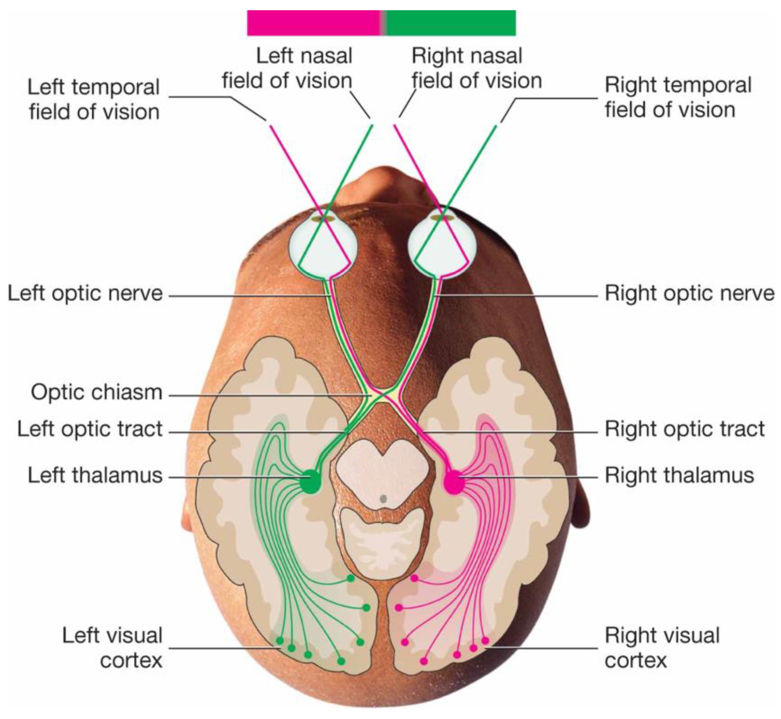
2.1. Evolution and Functionality of the Visual System

Erclik et al. [10] discussed eye evolution with the neuron as a unit of homology. There exist unusual neural cell-type homologies (genetic similarities) between Drosophila visual systems and vertebrate neural systems. These similarities were used to develop models that characterize the evolution of visual systems. In the first model, the neurons of the higher vertebrate retina have common-origin based similarities with the rhabdomeric cell types found in insects and the ciliary cell types found in lower vertebrates. It was suggested that the complex vertebrate retina has evolved from the merging of two evolutionary branches. The second model, as discussed by Erclik et al., is based on the genes involved in photoreceptor-target neuron development, and the model postulated that common ancestors of vertebrates and flies possessed good vision systems.
Human vision is a biologically intricate process involving several mechanisms that are still not understood by researchers. Kolb et al. [11,12] described the basics of the human vision system in two articles that serve as useful introductory reading on the topic. They described how several millions of photoreceptors are packed together in a tightly knit network in the retina. This complex neural network is contained within a half-millimeter-thick film of tissue at the back surface of the eye. The authors illustrated the retina as a three-layered cake with one layer of neurons and two filling layers of synapses. It is accepted that there are two basic kinds of photoreceptors, namely rods and cones. The cones are further subdivided based on light wavelength into two types, long- and short-wavelength sensitive cells, which are observed in most mammals. There is a third wavelength-sensitive cone in primates; it is similar to the long-wavelength cone type but slightly more sensitive in the green wavelength. This three-color detection range is observed in humans and other primates and is known as trichromacy or tri-variant color vision. Many other species, such as reptiles, birds, and fish, have one or two more types of color sensitive cones [13,14]. To reduce complexity, this research excluded images with color distributions, addressing images with black and white contrasts only.
Rossi and Roorda [15] established a relationship between the cone spacing and visual resolution in the human fovea. It was shown that at the foveal center, image resolution is limited by cone spacing, but outside the foveal center, visual resolution is better correlated with the density of midget retinal ganglion cells. In further exploration of the limitations of human vision, Hall et al. [16] studied human visual perception of camouflaged objects under various conditions. They studied three stages of predation—detection, identification, and capture. Contrary to previous assumptions, they observed that the motion of a camouflaged object did not always break its camouflage; especially when the object was surrounded by similar objects (such as animals in a herd) or similar moving distractors, the camouflage was still effective.
Randel et al. [17] studied the interactions of photoreceptors and motor neurons in annelid Platynereis larva’s four-eyed visual system through observation of visual phototaxis (bodily motion in response to light stimuli). They argued that image-forming camera-like eyes may have evolved via several intermediate stages, beginning with light- and dark-field detection. The collected data suggested that during photoreceptor development, connections to the neural cells (primary interneurons, which connect the photoreceptors to the motor neurons) become stronger. Unused interneurons were gradually eliminated.

2.2. Visual Learning, Movement, and Memory

There is strong evidence, as proposed here, to suggest that image and eye movement play key roles in visual learning, which involves the strengthening of the brain’s neural connections to the retinal photoreceptors. Marr and Poggio [18] developed a computational theory of human stereo vision. They followed similar logic to ours, visualizing beams emanating from each eye and detecting the right intersection. Images were analyzed through channels of various coarseness resolutions, and the corresponding channels from the two eyes were matched through disparity values on the order of the channels’ resolutions. According to them, the memory roughly preserves disparity-based depth information either during the scanning of a scene with differential eye movements or during the movement of the objects of interest. Similarly, Armson et al. [19] observed that eye movements promote the retrieval of spatiotemporal detail memories. Eye movement helps to recapitulate the temporal order of previously viewed space-based visual content.
Ryan et al. [20] noted that visual exploration served to build and recollect memories. More details from the past were retrieved when similar scenarios were shown or visited. Reciprocally, past memory increased the efficacy of the current visual exploration. They described neurodegeneration detection with eye-movement-based analysis. They observed that vision processing is linked to memory, and perception of an image can be used to recall past events from memory.
Montgomery and Young [1] observed that unlike hearing, which matures in a month after birth, the vision system develops more slowly over 6 to 8 months, at which point the baby sees the surroundings nearly as well as an adult. While newborns’ eyes are physically capable of seeing normally at birth, their brains are not ready to process the sudden massive influx of visual information, so images stay fuzzy for several months. Our paper illustrates this development with mathematical procedures. As the brain develops, so does the ability to see clearly, providing the tools the baby needs to comprehend and navigate its surroundings. Sakai [21] explained this phenomenon through a process called synaptic pruning, which shapes visual processing with improved neural wiring. It was observed that at birth, an infant has more neurons than an adult. Over the course of development, the neural circuits that are most used are strengthened and maintained, while the less used connections become weakened and fade. Our work focuses on this connection building process between the retinal space and the logical space in the brain and explores the possibility of extending that knowledge to distributed sensor technology.
Neural circuits adapt to various contexts throughout the visual training process. NIH [22] observed that most neuroscientists previously thought humans were born with a fixed number of neurons that remained constant throughout life. Scientists believed that adding any new neurons would disrupt the flow of information in the neural circuit and could disable the brain’s network system. However, more recent research indicates that children continuously produce new neurons to help build new pathways called neural circuits. Earlier in 1962, scientist Joseph Altman, as noted by the referenced NIH publication, supported this new theory of new connectivity as evidenced by neurogenesis (the birth of neurons) in the hippocampus of the adult rat brain, which modified the neural structure based on training and expertise. It was later reported that newborn neural connections migrated from their birthplace in the hippocampus to other parts of the brain. In 1979, research findings by another scientist, Michael Kaplan (as reported by the NIH publication), supported Altman’s findings in the rat brain; these discoveries in the human adult brain were surprising to several researchers, who did not think neurogenesis was possible for humans. In another example, scientists tried to understand how birds learn to sing and suggested that new neural circuits were formed in the brains of adult birds [23]. In a series of experiments, Fernando Nottebohm and his research team [24], as reported by NIH, showed that the forebrains of male canaries dramatically increased the numbers of neurons during the mating season (in which the birds invented new songs to impress female birds). These studies indicate that neural connections are not fixed, but rather adapt in response to various stimuli and activities.
In further support of the findings by NIH that the human brain is not a static device, Michelon [25] discussed the notion of plasticity, i.e., the brain’s capacity to change with learning. It is a widespread myth that neural connections in the brain become increasingly rigid with age; however, current progress in brain imaging indicates that the brain continually changes through learning. These learning-based changes happen mostly at the interneuron connections. New neural connections are formed, and the internal structures of the existing synapses change continuously. Furthermore, expertise in a field can make a specific part of the brain grow. For instance, London taxi drivers are found to have a larger hippocampus than London bus drivers; this is because the hippocampus is responsible for handling complex spatial information. This skill is used more often by taxi drivers, who have no fixed path and must adapt to traffic, congestion, smaller streets, different destinations, and the varying needs of their passengers, than by bus drivers, who repetitively follow a limited set of fixed routes [26].
Polat et al. [27] discussed training the brain to improve the aging eye (Presbyopia). They developed a vision training method that was found to improve contrast detection thresholds at all three spatial frequencies, indicating that the aging brain retains enough plasticity to overcome biological deterioration. However, an improved detection of grey levels through training was difficult to achieve. Still, this work was the first to show that vision improvements through training were attributable not to the optical performance of the eye but to the increased efficiency of neural processing. They found that the visual system can improve its perception of blurred images using applied cognition.

2.3. Optical Illusion and Visual Learning

Optical illusions provide a means to uniquely characterize human vision, and they further attest to the importance of neural processing above optical performance in visual perception. Thibos [28] modeled human image processing comprising two concatenated filters, the first being optical and the second being neural. Evidence of aliasing (signal frequency distortion) in human vision was discussed and illustrated through a simulation of an aliased neural image in the peripheral visual field. Optical illusion does not happen in digital image processing; therefore, it can be argued that the analysis of these illusions may provide guidance toward understanding intelligent image processing and perception.
In support of the previous discussions regarding the link between perception and memory, Rizzi and Bonanomi [29] observed that the human visual system does not register objective reality; instead, it modifies the appearance of a scene by adjusting to its content using visual memory. For this reason, optical illusions may provide important insight into the less understood inner mechanisms of the human visual system. Heller et al. [30] observed that optical illusion is not truly optical but instead is related to perception and analysis. Despite its name, the same illusion was observed between sighted and visionless participants in their study. They compared the Müller-Lyer illusions with sighted and congenitally blind people and found not only that blind testers experienced a similar illusion when they processed the images using touch, but also that the touch-based illusion could be stronger than the visual illusion on the same graphical layouts.
Williams and Yampolskiy [31] created a dataset of images that play tricks on visual perception, including causing misjudgment on color, size, alignment, and movement. Robinson et al. [32] explained brightness illusions with spatial filtering and local response normalization, illustrating that the intensity illusions could be captured by mathematical models. Filtering and changes in intensity scales were used to simulate the observed intensity mismatches, but no biological response was discussed to justify the illusions. Other animals can also experience optical illusions, and not all animals experience the same optical illusion from the same image; for example, Watanabe et al. [33] observed that pigeons’ perception of the Zollner illusion is reversed from that of humans. The reason for this discrepancy, it was argued, was that human perception has both assimilation and contrast effects, whereas pigeons’ perception only has assimilation effects.
Coren and Girgus [34] tested relative efficiency on the parametric variation of the Müller-Lyer and Ebbinghaus figures. They concluded that the methods of average error, reproduction, and graded series techniques were better than the rating scale and magnitude estimation techniques. Franz [35] worked on the neuropsychological measure of perception and found that the same neuronal signals were responsible for common illusions, size estimation, and grasping. The causes for optical illusions are still not fully understood, but it is known that they are not truly “optical” as the name indicates; rather, they are related to the perception and processing of images in the brain. Given that illusions are one of the major discrepancies remaining between human and machine vision, a better understanding of the mechanisms behind illusions may provide new insight that could aid in the replication of human visual learning and the associated development of security and intelligence-based technologies.

2.4. Modeling and Analysis of the Human Vision System

Discussion of the physics of visual perception by Campbell and Marr [36] identified that any temporal or spatial stimulus could be characterized by its Fourier transform. The visual system was analyzed using band-pass filters on waveforms. It was found that the contrast threshold (minimum contrast required for the human eye to differentiate lines) was different for a sinusoidal grating compared to a square wave grating or a point source (like a star in the moonless sky). For similar frequencies, the differently shaped waveforms had different contrast thresholds. It was thus presumed that vision had frequency tuned channels, and this work provided band-pass characteristics of these channels.
McIlhagga and Mullen [37] used classification images to illustrate chromatic edge detectors in human vision. Chromatic (color-based) edge detectors appeared larger than the luminance (light-based) edge detectors, resulting in a lower spatial resolution in chromatic vision. Moreover, chromatic edges were sensitive to change in color (such as red vs. green or blue vs. yellow) than to the color itself.
Marr and Hildreth [38] developed a theory on edge detection as part of the artificial intelligence laboratory at MIT. Their theory was based on two parts—intensity differences within the same object and intensity changes due to surface discontinuities between different objects. They observed that an edge has a partly visual and partly physical meaning. Georgeson [39] argued that computational edge detection models can be broadly classified into either circular spatial filters or orientation selective filters. The oriented filters are not orientation detectors but rather are located spatial features.

2.5. Machine Learning
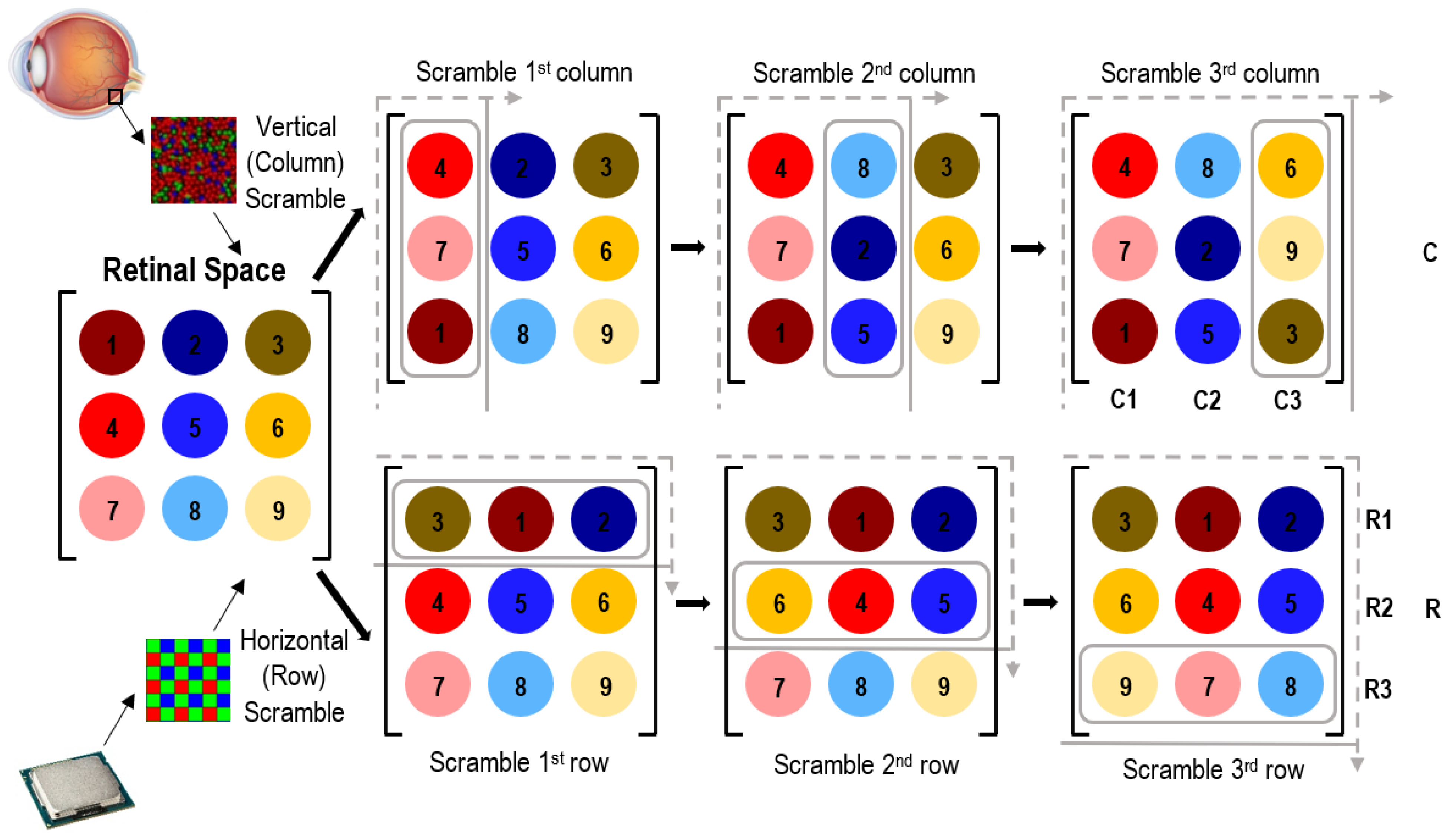
Object recognition is a major component of machine vision, and it requires machine learning methods; these methods may be improved using insight into the differences between human and machine visual learning. To characterize one of these differences, Garcia-Garibay and de Lafuente [40] analyzed the Müller-Lyre illusion through an artificial neural network. They argued that comparing line lengths in illusions is not as straightforward as it seems because visual systems process complete visual objects rather than local information. Our work is a step forward toward an intelligent visual system, and we hope to expand in the world of perception in the future. Krizhevsky [41] trained a large deep-convolutional neural network to classify 1.2 million images with an excellent error rate of 37.5%. Image analysis is highly complex, and the chosen technique included 60 million parameters and 650,000 neurons with five convolutional layers. Biological image processing and classification techniques are somewhat different from these digital techniques; our work explores the beginning of image reconstruction process, and hopefully this can be extended to image classifications later.
Zeman et al. [42] discussed the disparity between perception and objective reality. They implemented a technique called HMAX architecture, which uses an artificial network to perform linear classification of optical illusion defined in Müller-Lyre categories. Watanabe et al. [43] developed deep neural networks that were used to predict operational algorithms of the brain, including illusory rotational motion. They argued that in using sensory illusions as indicators of human perception, deep neural networks are expected to contribute significantly to the development of brain research.
Lades et al. [44] proposed a dynamic link architecture for object recognition. This link architecture, an extension of the classical artificial neural networks, used connection parameters between two neurons and provided a synaptic weight for signal transmission. This architecture is a self-organizing network with a positive feedback loop.
Talbi et al. [45] proposed a genetic quantum algorithm to perform an image registration for a vision system. The proposed system catalogued images coming from different sensors. Forcen et al. [46] illustrated spatial pooling as an important step in computer vision systems. This process combines neighboring descriptors to obtain a descriptor for a given region. Their technique used local image features for scene detection. In 1981, Grimson [47] presented a computational theory of visual surface interpolation, an impressive feat considering the lack of tools available at the time compared to what exists today. The work attempted to computationally interpolate complete surfaces from a discrete set of points; this was achieved through the calculation of variations associated with problems of minimum energy. Minimum energy could be the driving force for evolution-based biological systems, but available information is not yet sufficient for this determination. A year earlier, in 1980, Grimson [48] published ideas on implementing human stereo vision in a computer framework. The first step of the stereo vision implementation was fixing the two-eye position with two zero-crossing descriptions. We did not extend our work to stereo imaging, but the discussion is provided as a guidance for future extension of our work.
Bergstra et al. [49] proposed a hyperparameter optimization algorithm to improve on face matching verification, face identification, and object recognition. These image processing capabilities seem to be difficult to achieve in digitized images, but our brain performs them effortlessly and with low power consumption; our work is a step toward understanding how this processing is carried out in the brain. Tsuda and Ratsch [50] developed a linear program based technique for image reconstruction. Their technique was used for de-noising the image for further processing and was based on existing statistical approaches. They concluded that the power of convex optimization was not fully utilized in image processing and that there is room for advancement. Bhusnurmath [51] studied convex optimization techniques to minimize energy in computer vision. This work effectively parallelized the linear program code on CPU and GPU with giga flops capabilities. This was complex and innovative work, but the human eye can achieve the same outcome without significant power and most likely with a different technique. Our work is a step forward in the direction of understanding the biological mechanisms behind human visual perception and how they may be used in the advancement of technological applications. Clearly, there is much progress to be made in understanding the biological mechanisms behind human visual perception; hopefully, this work can help to replicate these intelligent visual processes so that they can be used for the advancement of technological applications, such as spatially calibrating randomly placed sensors.

3. Methodology

The objective of this work is to reverse-engineer the connection between the brain’s processing unit (the “logical space”) and the photoreceptors in the eye (the “retinal space”). It is assumed that there is one-to-one connectivity between the locations; this may be a valid assumption for the fovea centralis [15]. For simplicity, optical receptors are placed in a uniformly spaced XY grid, and it is assumed that the edges in training images are aligned with either the x- or y-axis. Inclined edges and nonuniform sensor distribution may provide a more realistic representation of the true retinal configuration, but additional research is required to incorporate these complex effects.
Figure 3 highlights the basic difference between a digital camera and a human eye. The digital camera’s photosensor is manufactured with painstaking perfection to produce repeatable results. Each pixel is the same, and its exact location is in-built and identical from one sensor to the next, resulting in identical “perceived” images between different sensors. The software driving the image processing does not need to calibrate the pixel locations. Conversely, the human eye is different from one individual to another. The rods and cones are packed differently, and as a result they may produce different perceptions of the same visual stimulus, as depicted in Figure 3a. Thus, the brain must calibrate its neural connections with these unnumbered, haphazardly distributed photoreceptors in order to achieve accurate image perception. Interestingly, previous research did not question or test the accuracy of the perceived image layout (line configuration, relative positioning, shape and size) but only that of the hue and color consistency. We addressed the nonuniform distribution of photoreceptors and possibly how the brain reverse-engineers their locations. This knowledge may aid in the development of intelligent imaging technologies such as the spatial mapping of distributed sensors in smart cities and in hostile zones. The global GPS system may not be the optimal method for mapping large numbers of sensors, and in hostile zones it may not be desired to disclose GPS positions, in case the sensors are compromised.
This work documents the progress made in the simulation of retinal spatial mapping, which may be useful in further optimizing imaging technologies. It does not follow the conventional research paper format of analysis, model development, and results. Instead, we developed a hypothesis based on biological observations and adopted it to develop techniques and models that may be useful for engineering applications. Each section within the results and discussion illustrates a different concept and helps establish the technique needed to resolve the spatial mapping of sensors.
In this work, a memristor factor (MF) is used as a damper for the strengths of the connections in the neural circuit. The strength of a neural connection is iteratively updated as New Neural Connection Strength = (1 + MF × Previous Neural Connection Strength). This technique simulates the synaptic neural pruning that has been observed in biological research. The results indicate that a static image is not enough to map the retinal to logical connections. To build proper neural connections, it is shown that information from dynamic images is required.
The methodology presented here can be divided into two broad components, i.e., finding the neural connections and finding the neural node neighbors.

3.1. Finding the Neural Connections

Unlike in a digital camera, a retinal photoreceptor (the equivalent of a pixel in a camera sensor) is not initially calibrated in its spatial location. After an image is captured in the retina, the optical data are transported to the back of the brain for further processing. For vision to work properly, the brain’s visual neurons must be mapped to their corresponding retinal photoreceptors; the first two sections of the results discuss the neural training through which this connectivity is established. There are millions of photoreceptors in the retina. To simplify, let us assume a 2 × 2 matrix, i.e., [(R1,R2);(R3,R4)] on the retinal surface with four photoreceptors R1 to R4. These photoreceptors are connected to brain locations [(B1,B2);(B3,B4)]. These spaces are biologically connected to one another, but they do not provide information about the connections between individual cells (e.g., whether R1 is connected to B1 is not known to B1). They also do not provide information about the relative positions of R1, R2, R3, etc. In the first part of the research, the connectivity between R1 and B1, R2 and B2, and so on, are established using dynamic image features.
Let us say there is an edge in the image that excites R1 and R2. Due to a hardwired neural connection, both B1 and B2 will receive the excitation signals. Unless it is a point image, the brain cannot connect B1 to R1. This gets more complex when millions of sensors are working at the same time and when images are complex as well. The technique is explained for more complex environment in the results with numeric diagrams.

3.2. Finding the Neural Node Neighbors

After pairing the retinal locations with logical locations in the brain, neighborhood information is needed to process the image information. For example, to detect a line, the spatial sequence of photoreceptors is needed. A perturbation technique is developed here that uses image samples and trains the brain to identify the neighbors of photoreceptors. If we consider neighbors in x- and y-directions, R1 has R2 and R3 as neighbors, which can be detected by sampling images and moving them in x- and y-directions. For example, let us say there is point feature and only R1 is activated. In the next perturbation, the feature is moved by one unit in the x-direction. After that x-direction move, R2 becomes activated. From this exercise, the brain could decide that R2 is the right neighbor of R1. However, the training mechanism is more complex than that because there are millions of photoreceptors and thousands of features. The problem of neighbor detection is solved by statistical methods and a memristor factor. If the perturbation is continued, the number of times R2 is detected as the right neighbor of R1 is high; this is how the training technique is implemented.
A schematic of the perturbation technique is illustrated in Figure 4. Solid green locations are where the features are present in the image to activate the photosensors. The image is then perturbed in +1 position in the x-direction as shown. From this, the brain obtains the information that the dotted line locations are the right neighbors of the feature containing photoreceptors. However, it cannot determine who is the neighbor of whom just from one exercise like this. To determine the neighbors, the process is repeated with different images, that is, the solid green locations are varied but with the same density for the simulations. The number of images used is identified as iterations in this work. In this illustration, 25% (i.e., 4 out of 16 locations) of the domain allotted for initial features are populated and is controlled by a rounding adder (RA) in the computation. For the given configuration, RA is equal to 0.25.
The perturbation is continued in all four directions, namely +x, −x, +y, and −y. For illustrative purposes, the perturbation is taken as one unit with each iteration here; it is expected that this work will be expanded by others to include random perturbations and nonorthogonal movement, which are beyond the scope of this work at the time.

4. Results and Discussion

4.1. Failure of Spatial Reconstruction with Static Images

The objective of this section is to logically simulate the spatial mapping of photoreceptors in the brain. The sensor (photoreceptor) locations in the retina are designated in the retinal space matrix, as depicted in Figure 5. The task is to reconstruct this retinal spatial distribution in the brain’s neural network, which is referenced as the logical space. In a digital camera, the pixels are numbered in the chip, and so the software does not require this spatial calibration. Contrarily, in the biological vision system, the retinal space is not structured, and the logical space of the brain is not systematically numbered. It is hypothesized that the brain identifies common features such as an edge or colored area and then trains itself to reconstruct the tentative locations of the retinal space for image perception. We suppose that 9 sensors are laid out in a 3 × 3 matrix in the retina as depicted in the retinal space in Figure 5. Next, we assume horizontal and vertical edges are detected by the retina. We then suppose a vertical line of light activates the first column, which contains sensors 1, 4, and 7. The brain becomes aware that sensors 1, 4, and 7 are activated, but it will not know their correct order. The brain needs to determine this order to reconstruct the image. Here, we let the signals be arbitrarily scrambled into the order 4, 7, 1, which are activated in the presence of that edge. Similarly, the next two columns are activated by other edges and are scrambled as 8, 2, 5 and 6, 9, 3. In Python, this data structure is called a set; compared to an array, a corresponding set contains the same numbers, but unlike the array, it does not record any particular order for the numbers. In applying the same process along the horizontal direction, the horizontal edges will create scrambled rows [(3,1,2); (6,4,5); (9,7,8)], as illustrated in Figure 5.
Let us suppose that the static image information provided the brain the information that (8,2,5) are in the same column, and (3,1,2) are in the same row. Now, if we match this row and column at their shared point (2) and continue similarly adding on more rows and columns as illustrated in Figure 6 until the matrix is fully populated, the resulting reconstructed space satisfies the row and column sets (i.e., each row and column contains valid neighboring cells), but the whole set does not match the retinal space distribution (i.e., the cells are not in the correct order). This illustration demonstrates that the spatial mapping of sensors to the logical space using static images is not dependable; it may result in solutions that match the row and column sets but not the full matrix configuration.

4.2. Spatial Reconstruction with Moving Dynamic Images

Since the retinal space cannot be reliably reconstructed using static images alone, a hypothesis with moving edges is illustrated next. Figure 7 demonstrates the dynamic edge concept, in which moving images are used for spatial mapping of the retinal cells to their correct corresponding neural brain cells. If we take into consideration how the eye can detect eye movement direction and can correlate the expected corresponding image movement, then it can rearrange the scrambled columns by detecting which sensor is to the left and which is to the right. A similar method is performed in the orthogonal direction to order the rows from top to bottom. The middle matrix in Figure 7 depicts the alignment of the scrambled matrix after the vertical edge scan; the vertical line movement would identify that sensor 8 comes after 7, and 9 comes after 8, thus putting the columns in order. However, the vertical line cannot resolve the rows; a horizontal line (moving vertically) achieves this by identifying that sensor 4 comes after 1, and 7 comes after 4. When combined, these two processes perfectly reconstruct the retinal space. Thus, together, the vertical and horizontal scans of light stimuli can correctly reconstruct the retinal space in the logical brain space. This could not be achieved with static images, which leads to the conclusion that a moving reference is essential for the brain to place the retinal locations correctly in its logical space.

4.3. Intercept Method for Sensor ID Location

In the previous sections, it was demonstrated that a static image cannot help with identifying the sensor at a specific location; for proper sensor location identification, image or eye motion is required. The scanning of an image or view is now applied on a larger set of sensors. Figure 8 depicts the retinal space, in which each photosensor is marked with a unique color as an identifier. A horizontal scan of vertical edge lines creates scrambled datasets as shown at the top of Figure 8. The bag represents the “scrambling” of a row or column to obtain an unordered set of numbers; the rows and columns indicated by the bag contain all of their correct (same as retinal space) respective sensors, but they contain no information about the sequence or location of the sensors within the row/column. The vertical scan of horizontal edges is depicted in the lower portion of Figure 8. To better understand these scans, we can imagine a situation where the eye sees an edge, such as a corner or wall-ceiling intersection. With eye motion, that line is moved across the retinal space, allowing the brain to logically reconstruct the image as it enters the eye (before becoming scrambled along the neural pathways to the brain); this is the process by which these datasets are created. This may not truly be how the brain processes images, but it is a possible logical method that can be used for locating sensors in an array. The biological visual learning process is described in the next section.
If the scrambling process with this larger dataset seems confusing, it may help to revisit Figure 5, Figure 6 and Figure 7 with smaller datasets, as smaller datasets are easier to grasp and visualize.
Figure 9 depicts the reconstruction of the scrambled datasets. The reconstruction is simple in mathematical terms and can be used on orthogonally scanned datasets. The intercept of the vertical scrambled line and horizontal scrambled line gives the sensor ID at the intercept location. The sensor ID at a given location is (vertical scan dataset) ∩ (horizontal scan dataset). However, this mathematical operation does not occur in biological learning. Rather, the brain’s visual mapping process is better understood as a statistical sampling and an enabling of neural connections, as is described in the next section. Note that the set intersection technique depicted in Figure 9 is useful for laying out and locating large arrays of sensors without knowing where they were placed. The sensor locations can be detected logically through their collective response to visual input as is illustrated with retinal and logical nodes.

4.4. Statistical Learning by the Brain Based on Photosensor Response

Unlike what is described previously, the brain’s learning does not involve set theory and manipulation of number collections. Here, an attempt is made to simulate how the brain might untangle visual information and determine the spatial locations of the retinal photoreceptors. To understand that mechanism, a perturbation method is used as described in Section 3. The human eye is not rigid, and the image captured is constantly moving. For simplicity, it is assumed that an image on the retina is sequentially perturbed by one unit in the ±x direction and one unit in the ±y direction. As illustrated in Section 3, if light is shining on the (i,j) receptor, then due to perturbation (i − 1,j), (i + 1,j), (i,j − 1), and (i,j + 1) are also stimulated. This is a simplistic assumption but a step toward understanding the learning and adaptation that happen in the early stages of brain development. The problem is that when sensor (i,j) is stimulated, many other sensors in the retina are stimulated as well. To capture this effect in simulation, a random number of sensors are stimulated in the retinal space at a time, and that random set is repeated several times. For mathematical expression, these repeats are referred to as iterations. Each iteration uses a new image map on the retinal space. The number of sensors activated is controlled by a rounding adder (RA) in the Python code; RA = 0 in the model signifies that no sensors in the retinal space are receiving light, and RA = 1 means all sensors in the retinal space are excited.
It was proven by experiments that the biological brain is not a static neural structure; rather, it continuously evolves and makes new connections through a phenomenon known as brain plasticity [25]. Initially, all neurons of an infant’s brain are connected to each other, but over time, the most frequently connections strengthen and become established as viable connections, while the unused ones perish. This process of selective development in the brain’s neural circuits is called synaptic pruning [21]. A numerical model is developed here to study the process of synaptic pruning. The effect is similar to that of a memristor, as proposed by Chua [58]. A memristor is a theoretical circuit element that has a “memory” and this element allows it to adjust its resistance depending on its usage in the electrical circuit. There are existing studies on this component in the context of electrical circuits [59,60], but our work may be the first to apply the memristor analogy to synaptic pruning. The observed medical records, as cited previously, indicate that neural resistance decreases with usage, similar to a memristor circuit element.
As discussed in Section 3, a memristor factor (MF) was implemented as a dynamic factor for establishing strengths of neural connections. The strength of a connection between two nodes is iteratively updated as New Neural Connection Strength = (1 + MF × Previous Neural Connection Strength). There are no experimental data to validate the exact value of the MF, but as illustrated by the following figures, the numerical simulations indicate that the MF plays an important role in identifying viable connections in synaptic pruning. The MF used here indicates the residual effect of the previous usage added to the current neural connectivity.
Figure 10 illustrates the need for a memristor effect as used in synaptic pruning. The greater the column height, the more probable it is that the cell location represented by the column is a neighbor of sensor (4,4). The simulations are for 1000 iterations, meaning 1000 different images with perturbations are used. The image density is high (RA = 0.9). The memristor factor is applied in Figure 10b, in which it can be observed that the neighbors of the sensor located at (4,4) are more clearly identified. With memristor, the distant nodes’ connectivity strengths correctly drop to near zero. The neighbors are (3,4), (5,4), (4,5), and (4,3), and they all have high relative connectivity strength. Without the MF, as shown in Figure 10a, there is significant noise in the connectivity map.
Figure 11 depicts the infant stage training outcome of the simulated brain. Iterations represent the sample size (number) of images used for training. It was observed that with increased statistical sampling represented as iterations, the identities of a sensor’s neighbors become more distinguished. Like before, the presented results are for sensor (4,4). With increased training, the neighbors are more clearly identified. Neighbor information is needed for edge detection, for perception, and for visual grasping of the environment. An iteration count of 1000 means 1000 images were used for training; results show that neighbors of location (4,4) become more prominent with 5000 iterations. This simulation demonstrates that complex mathematical operations such as set intersection can be achieved through statistical sampling and memristor-like adjustments that model biological synaptic pruning. It is understood that the analyses performed here used simplified movements and sensor arrangements. Hopefully, others can see the opportunity to expand on this work and bring in the concept of perception that is missing in classical digital image processing.

5. Conclusions

In this study, we built a procedure for simulating visual spatial mapping with a hypothetical array of distributed sensors. The optical circuit of human vision was selected due the availability of relevant medical research and the recent development of intelligence-based theories. The objective of the research was to simulate the mapping of retinal photoreceptors to their associated brain cells, which enables perception and image processing. It was argued that the neural connection from one cone cell to its associated brain cell is not established at birth. The brain and eye work together along with the movement of the eye and head to learn the spatial distribution of the retinal photoreceptor cells. We found that static images are not suitable for training the brain to recognize visual sensor locations; rather, image movement or perturbation is required to decipher the relative locations of the photoreceptors. To simulate this phenomenon, we conducted a mathematical analysis using a number set-theory based intersection of two orthogonal image scans. Lastly, we demonstrated how set intersection is implemented by the brain through statistical sampling. We observed that a memristor, which is a special type of electrical component, may be analogous to the mechanisms involved in synaptic pruning. Synaptic pruning eliminates unused neural connections and strengthens the most frequently used connections. The proposed model effectively captures the neighbor detection of the retinal photosensors by the brain with repeated training on the images by perturbation.

Author Contributions

Conceptualization, S.D.; methodology, S.D.; validation, S.D. and M.W.; formal analysis, S.D. and M.W.; writing—original draft preparation, S.D.; writing—review and editing, M.W.; visualization, M.W.; supervision, S.D. All authors have read and agreed to the published version of the manuscript.

Funding

This research received no external funding.

Data Availability Statement

Data is contained within the article.

Conflicts of Interest

The authors declare no conflict of interest.

References

  1. Montgomery, N.; Young, P. Baby Sensory Development: Sight. 2019. Available online: https://www.babycenter.com/baby/baby-development/baby-sensory-development-sight_6508#:~:text=world%20around%20her.-,When%20it%20develops,as%20well%20as%20you%20do (accessed on 3 June 2021).
  2. Churchland, P.S. Is the Visual System as Smart as It Looks? Proceedings of the Biennial Meeting of the Philosophy of Science Association 1982, 2, 541–552. Available online: http://www.jstor.com/stable/192442 (accessed on 3 June 2021).
  3. Biology Forums Gallery Optic Nerve, Optic Chiasm, Thalamus, and Visual Cortex. Biology Forums. Available online: https://biology-forums.com/index.php?action=gallery;sa=view;id=13954 (accessed on 3 June 2021).
  4. Lin, J.; Tsai, J. The Optic Nerve and Its Visual Link to the Brain. Discovery Eye Foundation. 2015. Available online: https://discoveryeye.org/optic-nerve-visual-link-brain/#:~:text=In%20the%20brain%2C%20the%20optic,into%20objects%20that%20we%20see (accessed on 3 June 2021).
  5. Varadarajan, S.G.; Huberman, A.D. Assembly and Repair of Eye-to-Brain Connections. Curr. Opin. Neurobiol. 2018, 53, 198–209. [Google Scholar] [CrossRef]
  6. Goldman, B. Long-Distance Eye-Brain Connections, Partial Vision Restored for First Time Ever in a Mammal 2016. Stanford Medicine. Available online: https://scopeblog.stanford.edu/2016/07/11/long-distance-eye-brain-connections-partial-vision-restored-for-first-time-ever-in-a-mammal/ (accessed on 11 June 2021).
  7. Fritzsch, B.; Elliott, K.L.; Pavlinkova, G. Primary Sensory Map Formations Reflect Unique Needs and Molecular Cues Specific to Each Sensory System. F1000 Res. 2019, 8. [Google Scholar] [CrossRef] [PubMed]
  8. Morgan, J.L.; Berger, D.R.; Wetzel, A.W.; Lichtman, J.W. The Fuzzy Logic of Network Connectivity in Mouse Visual Thalamas. Cell 2016, 165, 192–206. [Google Scholar] [CrossRef] [Green Version]
  9. Walinga, J. Chapter 5.2 Seeing. In Introduction to Psychology; BC Campus: Vancouver, BC, Canada, 2014; ISBN 978-1-77420-005-6. Available online: https://opentextbc.ca/introductiontopsychology/ (accessed on 3 June 2021).
  10. Erclik, T.; Hartenstein, V.; McInnes, R.R.; Lipshitz, H.D. Eye Evolution at High Resolution: The Neuron as a Unit of Homology. Dev. Biol. 2009, 332, 70–79. [Google Scholar] [CrossRef] [Green Version]
  11. Kolb, H.; Fernandez, E.; Nelson, R. Webvision: The Organization of the Retina and Visual System. 2020. Available online: https://webvision.med.utah.edu/ (accessed on 3 June 2021).
  12. Kolb, H. Cone Pathways through the Retina. 2011. Available online: https://webvision.med.utah.edu/book/part-iii-retinal-circuits/cone-pathways-through-the-retina/#:~:text=Cone%20photoreceptors%20are%20the%20sensors,of%20light%20in%20the%20retina.&text=The%20circuitry%20whereby%20cone%20signals,at%20the%20outer%20plexiform%20layer (accessed on 3 June 2021).
  13. Emmerton, J.; Delius, J.D. Wavelength Discrimination in the “Visible” and Ultraviolet Spectrum by Pigeons. J. Comp. Physiol. A 1980, 141, 47–52. [Google Scholar] [CrossRef] [Green Version]
  14. Davies, W.L.; Cowing, J.A.; Carvalho, L.S.; Potter, I.C.; Trezise, A.E.O.; Hunt, D.M.; Collin, S.P. Functional Characterization, Tuning, and Regulation of Visual Pigment Gene Expression in an Anadromous Lamprey. FASEB J. 2007, 21, 2713–2724. [Google Scholar] [CrossRef] [Green Version]
  15. Rossi, E.A.; Roorda, A. The Relationship between Visual Resolution and Cone Spacing in the Human Fovea. Nat. Neurosci. 2010, 13, 156–157. [Google Scholar] [CrossRef] [Green Version]
  16. Hall, J.R.; Cuthill, I.C.; Baddeley, R.; Shohet, A.J.; Scott-Samuel, N.E. Camouflage, Detection and Identification of Moving Targets. Proc. Biol. Sci. 2013, 280, 1–7. [Google Scholar] [CrossRef] [Green Version]
  17. Randel, N.; Asadulina, A.; Bezares-Calderon, L.A.; Veraszto, C.; Williams, E.A.; Conzelmann, M.; Shahidi, R.; Jekely, G. Neuronal Connectome of a Sensory-Motor Circuit for Visual Navigation. eLife 2014, 3. [Google Scholar] [CrossRef]
  18. Marr, D.; Poggio, T. A Computational Theory of Human Stereo Vision. Proc. R. Soc. Lond. B. 1979, 204, 301–328. [Google Scholar] [CrossRef]
  19. Armson, M.J.; Diamond, N.B.; Levesque, L.; Ryan, J.D. Vividness of Recollection Is Supported by Eye Movements in Individuals with High, but Not Low Trait Autobiographical Memory. Cognition 2021, 206. [Google Scholar] [CrossRef]
  20. Ryan, J.D.; Shen, K.; Liu, Z.-X. The Intersection between the Oculomotor and Hippocampal Memory Systems: Empirical Developments and Clinical Implications. Ann. N. Y. Acad. Sci. 2020, 1464, 115–141. [Google Scholar] [CrossRef] [PubMed] [Green Version]
  21. Sakai, J. How Synaptic Pruning Shapes Neural Wiring During Development and, Possibly, in Disease. Proc. Nat. Acad. Sci. USA 2020, 117. [Google Scholar] [CrossRef] [PubMed]
  22. Office of Communications and Public Liaison Brain Basics: The Life and Death of a Neuron. 2019. Available online: https://www.ninds.nih.gov/Disorders/Patient-Caregiver-Education/life-and-death-neuron (accessed on 3 June 2021).
  23. Barnea, A.; Pravosudov, V. Birds as a Model to Study Adult Neurogenesis: Bridging Evolutionary, Comparative and Neuroethological Approches. Eur. J. Neurosci. 2011, 34, 884–907. [Google Scholar] [CrossRef]
  24. Nottebohm, F. Why Are Some Neurons Replaced in Adult Brain? J. Neurosci. 2002, 22, 624–628. [Google Scholar] [CrossRef] [PubMed]
  25. Michelon, P. Brain Plasticity: How Learning Changes Your Brain. Sharp Brains. 2008. Available online: https://sharpbrains.com/blog/2008/02/26/brain-plasticity-how-learning-changes-your-brain/ (accessed on 3 June 2021).
  26. Maguire, E.A.; Woollett, K.; Spiers, H.J. London Taxi Drivers and Bus Drivers: A Structural MRI and Neuropsy-chological Analysis. Hippocampus 2006, 16, 1091–1101. [Google Scholar] [CrossRef]
  27. Polat, U.; Schor, C.; Tong, J.-L.; Zomet, A.; Lev, M.; Yehezkel, O.; Sterkin, A.; Levi, D.M. Training the Brain to Overcome the Effect of Aging on the Human Eye. Sci. Rep. 2012, 278. [Google Scholar] [CrossRef] [PubMed] [Green Version]
  28. Thibos, L.N. Image Processing by the Human Eye. In Proceedings of the SPIE 1989 Symposium on Visual Communications, Image Processing, and Intelligent Robotics Systems, Philadelphia, PA, USA, 1 November 1989. [Google Scholar] [CrossRef]
  29. Rizzi, A.; Bonanomi, C. The Human Visual System Described through Visual Illusions. In Colour Design; Woodhead Publishing: Sawston, UK, 2017; pp. 23–41. [Google Scholar] [CrossRef]
  30. Heller, M.A.; Brackett, D.D.; Wilson, K.; Yoneyama, K.; Boyer, A.; Steffen, H. The Haptic Muller-Lyer Illusion in Sighted and Blind People. Perception 2002, 31, 1263–1274. [Google Scholar] [CrossRef] [PubMed]
  31. Williams, R.M.; Yampolskiy, R.V. Optical Illusions Images Dataset. 2018. Available online: https://arxiv.org/abs/1810.00415 (accessed on 3 June 2021).
  32. Robinson, A.E.; Hammon, P.S.; de Sa, V.R. Explaining Brightness Illusions Using Spatial Filtering and Local Response Normalization. Vis. Res. 2007, 47, 1631–1644. [Google Scholar] [CrossRef] [PubMed] [Green Version]
  33. Watanabe, S.; Nakamura, N.; Fujita, K. Pigeons Perceive a Reversed Zollner Illusion. Cognition 2011, 119, 137–141. [Google Scholar] [CrossRef]
  34. Coren, S.; Girgus, J.S. A Comparison of Five Methods of Illusion Measurement. Behav. Res. Methods Instrum. 1972, 4, 240–244. [Google Scholar] [CrossRef] [Green Version]
  35. Franz, V.H. Manual Size Estimation: A Neuropsychological Measure of Perception? Exp. Brain Res. 2003, 151, 471–477. [Google Scholar] [CrossRef] [PubMed]
  36. Campbell, F.W.; Marr, D. The Physics of Visual Perception and Discussion. Philos. Trans. R. Soc. Lond. Ser. B Biol. Sci. 1980, 290, 5–9. Available online: www.jstor.org/stable/2395412 (accessed on 3 June 2021).
  37. McIlhagga, W.; Mullen, K.T. Evidence for Chromatic Edge Detectors in Human Vision Using Classification Images. J. Vis. 2018, 18, 1–17. [Google Scholar] [CrossRef] [PubMed] [Green Version]
  38. Marr, D.; Hildreth, E. Theory of Edge Detection. Proc. R. Soc. Lond. B. Biol. Sci. 1980, 207, 187–217. [Google Scholar] [CrossRef] [PubMed]
  39. Georgeson, M.A. Human Vision Combines Oriented Filters to Compute Edges. Proc. Biol. Sci. 1992, 249, 235–245. [Google Scholar] [CrossRef]
  40. Garcia-Garibay, O.B.; de Lafuente, V. The Muller-Lyer Illusion as Seen by an Artificial Neural Network. Front. Comput. Neurosci. 2015. [Google Scholar] [CrossRef] [Green Version]
  41. Krizhevsky, A.; Sutskever, I.; Hinton, G.E. ImageNet Classification with Deep Convolutional Neural Networks; University of Toronto: Toronto, ON, Canada, 2012; Available online: https://www.cs.toronto.edu/~kriz/imagenet_classification_with_deep_convolutional.pdf (accessed on 3 June 2021).
  42. Zeman, A.; Obst, O.; Brooks, K.R. Complex Cells Decrease Errors for the Muller-Lyer Illusion in a Model of the Visual Ventral Stream. Front. Comput. Neurosci. 2014. [Google Scholar] [CrossRef] [PubMed] [Green Version]
  43. Watanabe, E.; Kitaoka, A.; Sakamoto, K.; Yasugi, M.; Tanaka, K. Illusory Motion Reproduced by Deep Neural Networks Trained for Prediction. Front. Psychol. 2018. [Google Scholar] [CrossRef] [Green Version]
  44. Lades, M.; Vorbruggen, J.C.; Buhmann, J.; Lange, J.; Malsburg, C.; Wurtz, R.P.; Konen, W. Distortion Invariant Object Recognition in the Dynamic Link Architecture. IEEE Trans. Comput. 1993, 42. [Google Scholar] [CrossRef] [Green Version]
  45. Talbi., H.; Draa, A.; Batouche, M.C. A Genetic Quantum Algorithm for Image Registration. In Proceedings of the 2004 International Conference on Information and Communication Technologies, Damascus, Syria, 23 April 2004. [Google Scholar] [CrossRef] [Green Version]
  46. Forcen, J.I.; Pagola, M.; Barrenechea, E.; Bustince, H. Learning Ordered Pooling Weights in Image Classification. Neorocomputing 2020, 411, 45–53. [Google Scholar] [CrossRef]
  47. Grimson, W.E.L. A Computational Theory of Visual Surface Interpolation. Philos. Trans. R. Soc. Lond. Ser. B Biol. Sci. 1982, 298, 395–427. [Google Scholar] [CrossRef]
  48. Grimson, W.E.L. A Computer Implementation of a Theory of Human Stereo Vision. Philos. Trans. R. Soc. Lond. Ser. B Biol. Sci. 1981, 292, 217–253. [Google Scholar] [CrossRef]
  49. Bergstra, J.; Yamins, D.; Cox, D.D. Making a Science of Model Search: Hyperparameter Optimization in Hundreds of Dimensions for Vision Architectures. In Proceedings of the 30th International Conference on Machine Learning, Atlanta, GA, USA, 16–21 June 2013; Available online: http://proceedings.mlr.press/v28/bergstra13.pdf (accessed on 3 June 2021).
  50. Tsuda, K.; Ratsch, G. Image Reconstruction by Linear Programming. IEEE Trans. Image Process. 2005, 14, 737–744. [Google Scholar] [CrossRef]
  51. Bhusnurmath, A. Applying Convex Optimization Techniques to Energy Minimization Problems in Computer Vision. Ph.D. Thesis, University of Pennsylvania, Philadelphia, PA, USA, 2008. Available online: https://www.cis.upenn.edu/~cjtaylor/PUBLICATIONS/pdfs/BhusnurmathPHD08.pdf (accessed on 3 June 2021).
  52. Tefi Shutter Stock Human Eye Diagram. Available online: https://www.shutterstock.com/image-illustration/human-eye-anatomy-detailed-illustration-isolated-174265226 (accessed on 3 June 2021).
  53. Vaiciulaityte, G. You’ll Be Amazed How People with Color Blindness See the World. Bored Panda. Available online: https://www.boredpanda.com/different-types-color-blindness-photos/?utm_source=google&utm_medium=organic&utm_campaign=organic (accessed on 3 June 2021).
  54. Kwan, C.; Chou, B. Further Improvement of Debayering Perfromance of RGBW Color Filter Arrays Using Deep Learning and Pansharpening Techniques. J. Imaging 2019, 5, 68. [Google Scholar] [CrossRef] [Green Version]
  55. Zhang, F.; Kurokawa, K.; Lassoued, A.; Crowell, J.A.; Miller, D.T. Cone Photoreceptor Classification in the Living Human Eye from Photostimulation-Induced Phase Dynamics. Proc. Natl. Acad. Sci. USA 2019, 116, 7951–7956. [Google Scholar] [CrossRef] [Green Version]
  56. Chulovskyi, Y. Shutterstock Wonderful Autumn Landscape. Available online: https://www.shutterstock.com/image-photo/wonderful-autumn-landscape-beautiful-romantic-alley-1911646903 (accessed on 3 June 2021).
  57. 7th Son Studio Shutterstock Close up CPU Upside Isolated on White. Available online: https://www.shutterstock.com/image-photo/close-cpu-upside-isolated-on-white-121109950 (accessed on 3 June 2021).
  58. Chua, L.O. Memristor- The Missing Circuit Element. IEEE Trans. Circuit Theory 1971, 18, 507–519. [Google Scholar] [CrossRef]
  59. Abraham, I. The Case for Rejecting the Memristor as a Fundamental Circuit Element. Nat. Sci. Rep. 2018. [Google Scholar] [CrossRef] [PubMed]
  60. Strukov, D.B.; Snider, G.S.; Stewart, D.R.; Williams, R.S. The Missing Memristor Found. Nature 2008, 453. [Google Scholar] [CrossRef] [PubMed]
Figure 1. Schematic of the human vision system (image courtesy of Biology Forums Gallery. Adapted from ref. [3]).
Electronics 10 01443 g001
Figure 2. Retinal cell network (image courtesy of open access. Adapted from ref. [9]).
Electronics 10 01443 g002
Figure 3. Human vs. machine visual perception (information and image courtesy of open access. Adapted from refs. [52,53,54,55,56,57]).
Electronics 10 01443 g003
Figure 4. Schematic of the perturbation technique.
Electronics 10 01443 g004
Figure 5. Image reconstruction from retinal space to brain’s logical space (processor and eye image courtesy of open access [52,54,55,57]).
Electronics 10 01443 g005
Figure 6. Inaccurate reconstruction of photoreceptor locations using static images.
Electronics 10 01443 g006
Figure 7. Orthogonal image scans to identify correct spatial orientation of photoreceptors.
Electronics 10 01443 g007
Figure 8. A large retinal space packaged in different sets based on vertical and horizontal edges.
Electronics 10 01443 g008
Figure 9. Reconstruction of the retinal space on logical space by intersection of number sets.
Electronics 10 01443 g009
Figure 10. Effect of memristor factor on neighbor identification for sensor at (4,4).
Electronics 10 01443 g010
Figure 11. Effect of iteration count on neighbor identification for sensor (4,4).
Electronics 10 01443 g011
Publisher’s Note: MDPI stays neutral with regard to jurisdictional claims in published maps and institutional affiliations.

