A Novel Bottom-Up/Top-Down Hybrid Strategy-Based Fast Sequential Fault Diagnosis Method

Abstract

Sequential fault diagnosis is a kind of important fault diagnosis method for large scale complex systems, and generating an excellent fault diagnosis strategy is critical to ensuring the performance of sequential diagnosis. However, with the system complexity increasing, the complexity of fault diagnosis tree increases sharply, which makes it extremely difficult to generate an optimal diagnosis strategy. Especially, because the existing methods need massive redundancy iteration and repeated calculation for the state parameters of nodes, the resulting diagnosis strategy is often inefficient. To address this issue, a novel fast sequential fault diagnosis method is proposed. In this method, we present a new bottom-up search idea based on Karnaugh map, SVM and simulated annealing algorithm. It combines failure sources to generate states and a Karnaugh map is used to judge the logic of every state. Eigenvalues of SVM are obtained quickly through the simulated annealing algorithm, then SVM is used to eliminate the less useful state. At the same time, the bottom-up method and cost heuristic algorithms are combined to generate the optimal decision tree. The experiments show that the calculation time of the method is shorter than the time of previous algorithms, and a smaller test cost can be obtained when the number of samples is sufficient.

1. Introduction

Fault diagnosis is a crucial activity for systems with high safety and mission criticality requirements [1], such as spacecraft [2], military helicopters [3], and aircraft satellites [4]. With the system structure becomes more and more complex [5], how to quickly and low-costly isolate faults [6] becomes a difficult problem. To solve it, Somnath Deb and K.R. Pattipati proposed the multi-signal flow graph model based on AND/OR graph in [7], which make test sequence optimization problem convert to the analysis and processing problem of D-matrix. Because the model is close to the actual physical system [8], and the integration and verification of the model is relatively simple [9], researchers have done a lot on this [10].

Currently, there are mainly two methods of sequential fault diagnosis algorithms based on multi-signal flow graph. One is the top-bottom search strategy, that is, the decision tree is constructed from top to bottom. The initial object is all faults, and test points are selected for fault isolation. There are four kinds of algorithms: (1) Greedy algorithm, whose time complexity is very low, but it is easy to fall into the local optimal solution because it does not consider the whole decision tree. (2) Heuristic search algorithm, which is also known as the AO* algorithm [11]. The heuristic search algorithm based on information theory was applied to generate the sub-tree to handle the imperfect tests existed extensively in the realistic systems [12]. To carry out iterative updating and construct the near-optimal diagnosis strategy, [13] proposed combining a rollout algorithm with information gain heuristic algorithms and [14] makes improvement in different search widths and depths. Several heuristic algorithms were proposed to find good strategies for large problem instances in [15]. The result of the algorithms is the global optimal solution, but when the heuristic value of each test point is close, it needs to traverse all cases, which takes a lot of time. In addition, with the increase of the number of faults, the time complexity increases exponentially and large storage is required. (3) Intelligent algorithm. In [16], the test sequencing problem was converted to search the minimal complete test sequencing based on the ant algorithm. Based on cuckoo search, [17] proposed an algorithm to generate optimized test sequences, which obtains 100% software coverage. These methods avoid the tedious logic design and seek rules from a large number of permutation and combination data. When the number of faults is large, it needs a lot of iterations and time is uncertain. (4) Hybrid algorithm, the combination of the Algorithms 1, 2 and 3 or the combination of these with other algorithms. Reference [18] proposed a new testing sequence optimization method based on AO* and dynamic programming to improve the efficiency of generating solutions. Reference [19] combined the greedy method with discrete binary particle swarm optimization (DPSO) to construct a test sequential tree. Reference [20] developed iterative algorithm called GLP(tau)S that uses genetic algorithms, LP tau low-discrepancy sequences of points and heuristic rules to find regions of attraction when searching a global minimum of an objective function. Another kind of method is bottom-up search strategy, that is, the fault tree is constructed from bottom to top [21]. The initial state is a single fault, continuous permutation and combination is carried until it is combined into a complete set of faults [22]. This avoids the repeated calculation of the same state, and has advantages in small-scale fault diagnosis. However, in large-scale fault diagnosis, the efficiency of the algorithm is low due to the generation of too many useless states.

To sum up, the main problem is that when the number of faults and test points is large, the time complexity of various algorithms is high [23] and the formation of decision tree is slow [21], that is NP hard problem [24]. Based on the above literature research, this paper proposes a new bottom-up/top-down hybrid strategy-based fast sequential fault diagnosis method. Firstly, a new bottom-up algorithm is established, which uses Karnaugh map, SVM [25] and simulated annealing algorithm [26] to decline the generation of useless state. It is suitable for the situation that the number of test points is more than the number of faults. Then the algorithm is combined with the cost heuristic search algorithm, which is suitable for the situation that the number of test points is less than the number of faults. This method makes the decision tree switch the algorithm according to the situation of nodes in the generation process, so as to improve the computational efficiency. Experimental results show that, compared with heuristic search algorithm and intelligent algorithm, the decision tree of this strategy has shorter generation time and guaranteed accuracy when dealing with large-scale fault dependency matrix.

The remainder of this paper is organized as follows. Section 2 describes the problem, Section 3 introduces the new proposed approach, Section 4 shows the comparative experiment with other algorithms, and Section 5 provides a summary.

2. Description of the Multi-Signal Flow Graph Combination Problem

In general, the testing sequencing problem is based on the information of failures, including five components:

• $S=\left\{S_1 ,S_2,\dots ,S_m\right\}$ is a set of statically independent failure associated with system, where $S_i$ means the ith fault state and m is the number of failure states;
• $P=\left\{P_1,P_2,\dots ,P_m\right\}$ is denoted as the priori probability vector according to the failure set $S$;
• $T=\left\{T_1,T_2,\dots ,T_n\right\}$ represents a finite set of n reliable binary outcome tests, where $T_j$ checks a subset of $S$;
• $C=\left\{C_1,C_2,\dots ,C_n\right\}$ is a set of tests cost based on time, manpower requirements or other economic factors;
• $D=\left[d_{ij}\right]$represents a binary matrix with $m\times n$, dimension to depict the relationship between the failure set and the test set, where $d_{ij}=1$ means the test $T_j$ is able to monitor failure state $S_i$ otherwise, $d_{ij}=0$.

The purpose of the sequential fault algorithm is to generate the optimal binary tree that can incur the least cost of fault separation.

As shown in

Table 1. Fault-test dependency matrix D1.

	${\mathit{T}}_1$	${\mathit{T}}_2$	${\mathit{T}}_3$
$S_1$	0	1	0
$S_2$	1	1	0
$S_3$	0	0	1
$S_4$	1	0	0

, the scale of D1 is $m\times n$, and the matrix is transformed into D2, D2 includes all binary digit combinations. It is shown in

Table 2. Fault-test dependency matrix D2.

	${\mathit{T}}_1$	${\mathit{T}}_2$	${\mathit{T}}_3$
$S_0^{*}$	0	0	0
$S_1^{*}=S_3$	0	0	1
$S_2^{*}=S_1$	0	1	0
$S_3^{*}$	0	1	1
$S_4^{*}=S_4$	1	0	0
$S_5^{*}$	1	0	1
$S_6^{*}=S_2$	1	1	0
$S_7^{*}$	1	1	1

.

Among them, S₀*, S₃*, S₅*, and S₇* are fictitious fault modules; if D2 is analyzed, the combination number of test sequence trees is calculated as shown in Equation (1).

$$Num={(n)}^{2^0}\ast {(n-1)}^{2^1}\ast \cdots \ast {(n-\left(n-1\right))}^{2^{m-1}}={\displaystyle \prod }_{i=0}^{n-1}{(n-i)}^{2^i}$$

(1)

The condition in which the fault in D1 can be completely isolated is shown in Equation (2).

$$m\le 2^n$$

(2)

As shown in Figure 1 and Figure 2, any test sequence tree of D1 is a subset of a test sequence tree of D2.

Different D-matrices of the same scale will generate optimal decision trees with different levels. In the meanwhile, its number of layers will not be larger than$n+1$. For the convenience of description and calculation, Figure 1 is changed to Figure 3, and the format of Figure 3 is a standard tree with $n+1$ layers, which is the same to Figure 2.

As shown in Figure 3, for any node at level K of the binary tree:

$$\begin{gathered} L_k={\sum }_{i=1}^{M_k}L{(M_i)}_{k\_left}\ast L{(M_i)}_{k\_right}\hspace{0.17em}\hspace{0.17em}\hspace{0.17em}\hspace{0.17em}\hspace{0.17em}\hspace{0.17em}\hspace{0.17em}\hspace{0.17em}\hspace{0.17em}\hspace{0.17em}\hspace{0.17em}\hspace{0.17em}\hspace{0.17em}\hspace{0.17em}\hspace{0.17em}\hspace{0.17em}\hspace{0.17em}\hspace{0.17em}\hspace{0.17em}\hspace{0.17em}(\mathrm{node} \mathrm{size} > 1) \\ {L}_k=1\hspace{0.17em}\hspace{0.17em}\hspace{0.17em}\hspace{0.17em}\hspace{0.17em}\hspace{0.17em}\hspace{0.17em}\hspace{0.17em}\hspace{0.17em}\hspace{0.17em}\hspace{0.17em}\hspace{0.17em}\hspace{0.17em}\hspace{0.17em}\hspace{0.17em}\hspace{0.17em}\hspace{0.17em}\hspace{0.17em}\hspace{0.17em}\hspace{0.17em}\hspace{0.17em}\hspace{0.17em}\hspace{0.17em}\hspace{0.17em}\hspace{0.17em}\hspace{0.17em}\hspace{0.17em}\hspace{0.17em}\hspace{0.17em}\hspace{0.17em}\hspace{0.17em}\hspace{0.17em}\hspace{0.17em}\hspace{0.17em}\hspace{0.17em}\hspace{0.17em}\hspace{0.17em}\hspace{0.17em}\hspace{0.17em}\hspace{0.17em}\hspace{0.17em}\hspace{0.17em}\hspace{0.17em}\hspace{0.17em}\hspace{0.17em}\hspace{0.17em}\hspace{0.17em}\hspace{0.17em}\hspace{0.17em}\hspace{0.17em}\hspace{0.17em}\hspace{0.17em}\hspace{0.17em}\hspace{0.17em}\hspace{0.17em}\hspace{0.17em}\hspace{0.17em}\hspace{0.17em}\hspace{0.17em}\hspace{0.17em}\hspace{0.17em}\hspace{0.17em}\hspace{0.17em}\hspace{0.17em}\hspace{0.17em}\hspace{0.17em}\hspace{0.17em}\hspace{0.17em}\hspace{0.17em}\hspace{0.17em}\hspace{0.17em}\hspace{0.17em}\hspace{0.17em}\hspace{0.17em}\hspace{0.17em}\hspace{0.17em}\hspace{0.17em}\hspace{0.17em}\hspace{0.17em}\hspace{0.17em}\hspace{0.17em}\hspace{0.17em}\hspace{0.17em}\hspace{0.17em}\hspace{0.17em}\hspace{0.17em}\hspace{0.17em}\hspace{0.17em}\hspace{0.17em}(\mathrm{node} \mathrm{size}=1) \end{gathered}$$

(3)

$$M_k={\displaystyle \sum }_{j=1}^n{A}_j$$

(4)

Node size refers to the number of $S$ contained in the node. If $A_j=0$, the node can be expanded by test point $T_j$, and if $A_j=1$, the node cannot be expanded by the test point $T_j$; $L_k$ is the number of combinations that the node can expand, and $M_k$ denotes the number of test points that can be used; $L{(M_i)}_{k\_left}$ and $L{(M_i)}_{k\_right}$ indicate the number of combinations that can be expanded by the two subnodes of the node under condition $M_i$, and the subnodes are located in the $k+1$ layer. To calculate the number of combinations of one node in k layer, we should obtain the number of combinations of the subnodes in $k+1$ layer firstly. Then, we should multiply the combination number of left and right subnodes based on the expansion of different test points. The whole calculation process is from bottom to top.

The combination number of test sequence trees generated by an $n\times m$ D matrix is $L_1$ ($L_1<Num$), and the initial value condition is $L_{n+1}=1$. $L_1$ is generated by iterative calculation of the formula in the standard tree according to Equations (3) and (4). Additionally, the expected cost J can be calculated as

$$J=P^{T}BC={\displaystyle \sum }_{i=1}^m{\displaystyle \sum }_{j=1}^n{b}_{ij}{p}_i{c}_j$$

(5)

where $B=\left[b_{ij}\right]$ is a binary matrix with dimensions of $m\times n$; $b_{ij}=1$ means that test $T_j$ is selected for the identification of fault state $S_j$ and otherwise, $b_{ij}=0$.

In summary, the problem of test sequence diagnosis based on a multi-signal flow graph aims to select the test sequence tree with the smallest J among$L_1$ types of test sequence trees. As m and n increase, the number of combinations $L_1$ greatly increases, which takes a long time to compare the cost of each tree and select the lowest, that is an NP-hard problem.

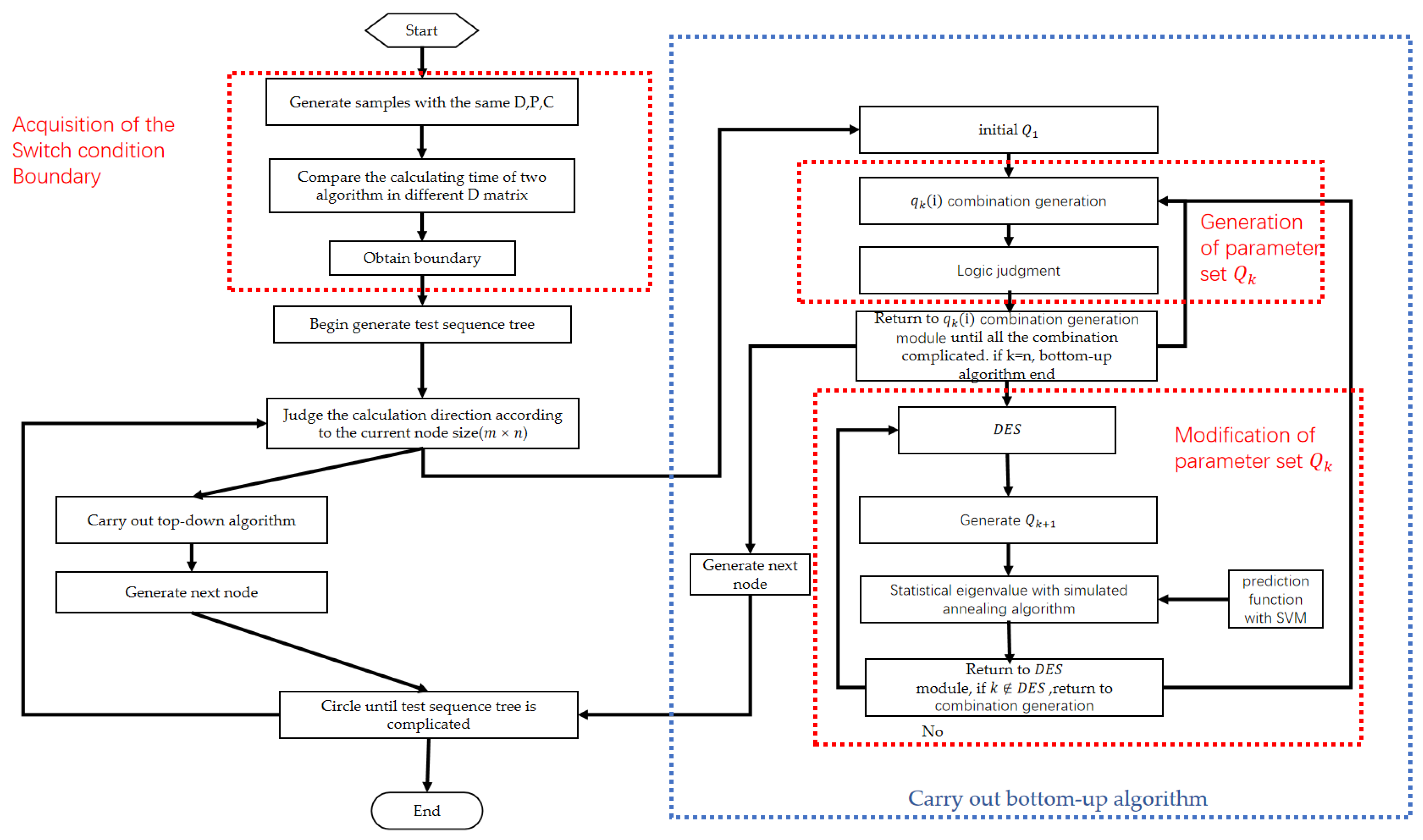
3. Proposed Sequential Fault Diagnosis Approach

The flow chart of the hybrid strategy is shown in Figure 4 and has three main parts: generation of parameter set, modification of parameter set and acquisition of switch condition boundary. The first two parts are novel bottom-up algorithms, which represent a great improvement compared with traditional bottom-up algorithms. Part three is used to define the switching conditions of the two algorithms, according to the size of the current node switch using two algorithms.

Firstly, a large number of samples are generated in accordance with the parameters of the test object. Both top-down and bottom-up algorithms are used to generate the optimal decision tree with these samples. Then, the time of the two algorithms is compared to obtain the switching condition. The next follows processing the test object. The size of the initial node is $m\times n$. The algorithm is selected according to the switching condition. After the algorithm is executed, the successor node is generated, and the algorithm is selected according to the situation of the successor node. It is then iterated until no successor nodes are generated. In addition, this flow chart is applicable to any top-down algorithms.

3.1. Generation of Parameter Set $Q_k$

The following definitions are applied:

• $q_k$: Any fault subset with size k of the fault complete set $S$, it contains three parts, k faults, k₁ and k₂ storage location information, and a series of Karnaugh map logic values, the length of which is n;
• $Q_k$: The set of all $q_k$. $q_k\left(\mathrm{i}\right)$ is used to denote the ith element in $Q_k$;
• $C_{q_k}$: If there are only k failures that belong to $q_k$ in the system, the minimum cost of testing is required;
• $P_{q_k}$: The sum of the failure rate of k failures in $q_k$.

$$P_{q_k}={\sum }_{i=1}^k{P}_i , \mathrm{where} S_i\in q_k$$

(6)

The optimal test sequence tree is a full binary tree, and thus any $q_k\left(k\ge 2\right)$ can be composed of $q_{k1}$ and $q_{k2}$, where $k_1+k_2=k\left(k_1\ge 1, k_2\ge 1\right)$. The calculation formula of $q_k$ is shown in Equation (7).

$$C_{q_k}=\frac{P_{q_{k1}}{C}_{q_{k1}}+P_{q_{k2}}{C}_{q_{k2}}}{P_{q_{k1}}+P_{q_{k2}}}+min\left\{C_{T_j}\right\}$$

(7)

where $T_{\begin{array}{c}j\\ \end{array}}$ refers to a test point that can separate $q_{k1}$ and $q_{k2}$ and should satisfy the conditions $\forall S_{i1}\in q_{k1},\forall S_{i2}\in q_{k2}, \exists d_{s_{i1}{T}_j}\ne d_{s_{i2}{T}_j}$; if $T_{\begin{array}{c}j\\ \end{array}}$ does not exist, $C_{q_k}=\infty$.

The flow chart of the bottom-up algorithm is shown in Figure 4. There are two main parts: one is the production of $Q_k$, and the other is the modification of $Q_k$.

By combining all the elements of $Q_{k1}$ and $Q_{k2}$ $(k_1+k_2=k$) in turn, this part calculates and generates $q_k$, judges the logic of $q_k$, compares various combinations that can generate $q_k$, and retains the combination with the least test cost until all combinations are generated, with $Q_k$ calculations completed. When $k=m$, the algorithm is end and decision tree can be obtained from $Q_m$.

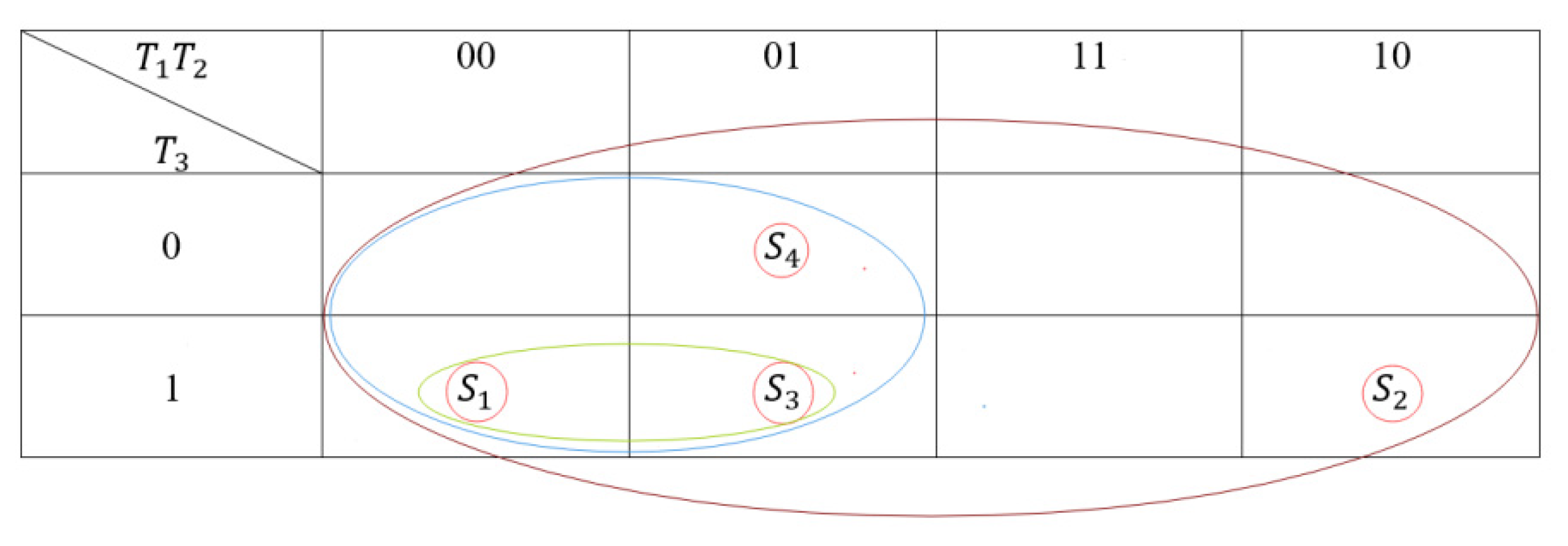
3.1.1. $q_k\left(\mathrm{i}\right)$ Combination Generation Module

Taking the fault-test dependency matrix in

Table 3. Fault-test dependency matrix.

	${\mathit{T}}_1$	${\mathit{T}}_2$	${\mathit{T}}_3$	P
$S_1$	0	0	1	0.1
$S_2$	1	0	1	0.2
$S_3$	0	1	1	0.3
$S_4$	0	1	0	0.4
C	1	1.5	2	-

as an example, the initial state $Q_1=\left\{S_1,S_2,S_3,S_4\right\}$. Any pairwise combination obtains $Q_2=\left\{S_1{S}_2,S_1{S}_3,S_1{S}_4,S_2{S}_3,S_2{S}_4,S_3{S}_4\right\}$. According to Formula (7), $C_{q_2}$ is $\left\{1, 1.5, 1.5, 1, 1, 2\right\}$. Next, we calculate $Q_3=\left\{S_1{S}_2{S}_3,S_1{S}_2{S}_4,S_1{S}_3{S}_4,S_2{S}_3{S}_4\right\}$; for example, $S_1{S}_2{S}_3$ is constructed in three ways: $S_1{S}_2+S_3,S_1{S}_3+S_2,S_2{S}_3+S_1$. According to Formula (7), the calculation cost is $\left\{2,2,\infty \right\}$, and the minimum value is 2. Similar to the above calculation, $C_{q_3}=\left\{2, 1.93, 2.75, 2.56\right\}$, $Q_4=\left\{S_1{S}_2{S}_3{S}_4\right\}$ is constructed in ten ways and compared with each other, and the minimization is $C_{q_4}=\left\{3.2\right\}$.

If all faults in the fault complete set s can be completely isolated, any subset of the fault complete set $q_k$ can also be completely isolated. According to permutation and combination

$$\left|Q_k\right|=C_m^k$$

(8)

$\left|Q_k\right|$ refers to number of $q_k$. The computing times of $q_k$ is shown in Equation (9).

$$Times=C_k^1+C_k^2+\cdots +C_k^{\left[k/2\right]}$$

(9)

where $\left[k/2\right]$ is the largest integer not exceeding $k/2$.

3.1.2. Logic Judgement Module

The output of the previous module calculates the state of redundancy, which should be deleted. For example, the state $S_2{S}_3{S}_4$ of $Q_3$; actually, regardless of the type of test sequence, the fault set S is not be separated into fault subset $S_2{S}_3{S}_4$. States such as this are non-logical items, and by eliminating the non-logical items to decrease|$Q_k$|, the combination number and calculation time can be greatly reduced. To judge the logic, a Karnaugh map is introduced. Taking the data in Table 3 as an example, the Karnaugh map is constructed with the test points as variables and the faults as logical values in Figure 5.

A complete segmentation method of the Karnaugh map is defined:

• Each circle conforms to the Karnaugh map circle rule, and its size is $2^y\left(0 \le \mathrm{y} \le \mathrm{n}\right)$;
• A large circle containing two smaller circles is treated as one circle;
• $S_i\left(1\le \mathrm{i}\le \mathrm{m}\right)$ each have a circle of size one;
• There are only two disjoint circles in a large circle;
• The maximum circle size is $2^n$, and it must exist.

Figure 5 presents the complete segmentation method of the Karnaugh map. According to the rule of Huffman code [27], a complete segmentation method of Karnaugh maps uniquely is consistent with a decision binary tree. Figure 6 corresponds to the decision tree of Figure 5.

In the Karnaugh map, a circle uniquely corresponds to a series of logical sequences composed of 0, 1 and d (d denotes “don’t care term”), and 0 and 1 denote the judgement results of the corresponding test points. where $q_k$ is composed of $q_{k1}$ and $q_{k2}$, and $q_k$ is a nonlogical item. The necessary and sufficient condition is described as follows:

• The circles of the Karnaugh map corresponding to $q_{k1}$ and $q_{k2}$ have no overlap;
• The circle of the Karnaugh map corresponding to $q_k$ does not contain $S_i$, $S_i\notin q_{k1}$ and $S_i\notin q_{k2}$.

As shown in Figure 5, $S_1$ corresponds to the logical value of 001, $S_4$ corresponds to the logical value of 010 according to the minimum item combination principle [28], and $S_1{S}_4$ corresponds to the logical value of 0dd. However, because $S_3$ is included in 0dd, $q_2=\left\{S_1{S}_4\right\}$ does not exist. According to the above theory, judging the logic of $q_k$ after it is generated and deleting nonlogic $q_k$ can reduce $\left|Q_k\right|$.

3.1.3. Entire Process of Generation of the Parameter Set

In summary, the entire process of generation of the parameter set $Q_k$ is shown in Algorithm 1.

Algorithm 1$Q_k$ production

1: $Q_k=Ø,k_1=1, i=1$; 2: $k_2=k-k_1$, take out one element in $Q_{k_1}$ and combine it with one element in $Q_{k_2}$ in turn; 3: Judge the logic of the combination result. If $q_k\left(\mathrm{i}\right)$ is a non-logic item, return to step 2. Otherwise, go to step 4; 4: Judge whether there is the same $q_k\left(\mathrm{i}\right)$ in $Q_k$. If not, it will be included, and $i=i+1$. Otherwise, compare the $C_{q_k}$ of the two and retain the smaller one;

5: Return to step 2, if all elements in step 2 have been combined, then $k_1=k_1+1, \mathrm{and}$ if $k_1>\left[k/2\right]$, the calculation is completed; otherwise return to step 2.

Furthermore, $\left|Q_k\right|$ can be estimated by Equations (10)–(12). $D_{xi}$ is defined as the ith column of the D-matrix with the size of $1\times m$. The self-generated number $SN$ is the number of $q_k$ that generated directly by $D$. $D_{xi}$ is equivalent to two fault subsets $q_{i_1}$ and $q_{i_2}(q_{i_1}+q_{i_2}=m)$. If $d_{ij}=0$, $S_i\in q_{i_1}$; otherwise, $S_i\in q_{i_2}$. For example, $D_{x1}$ is equivalent to one $q_1$ and one $q_3$shown in Table 3. Similarly, $D$ presented in Table 3 totally generates two $q_1$, two $q_2$ and two $q_3$. In addition, the combination number is defined as the number generated by the combination. The combination of $q_{k_3}$ and $q_{k_4}$ can also produce $q_k$ under the following conditions: if $S_i\in q_{k_3}$ and $S_i\in q_{k_4}$, then $S_i\in q_k (k<k_3, k<k_4)$. For example, the combination of $q_3=\{S_1{S}_3{S}_4$} in $D_{1i}$ and $q_3=\left\{S_1{S}_2{S}_3\right\}$ in $D_{3i}$ can produce $q_2=\left\{S_1{S}_3\right\}$.

$$CN={\displaystyle \sum }_{k_3=k+1}^m{\displaystyle \sum }_{k_4=k+1}^m\frac{C_{k_3}^k{C}_{m-k_3}^{k_4-k}\left|Q_{k_3}\right|\left|Q_{k_4}\right|}{C_m^k}$$

(10)

$CN$ refers to combination number. $Q_{k_3}$ and $Q_{k_4}$ have $\left|Q_{k_3}\right|\left|Q_{k_4}\right|$ kinds of combination and only $\frac{C_{k_3}^k{C}_{m-k_3}^{k_4-k}}{C_m^k}$ is the logical item. Considering that the sum of different $k_3$ and $k_4$ can be $k$, double summation is done. The combination process may produce repeated $q_k$ ($SN$ and $CN$ both produce it). The repetition rate$RR$ of $q_k$ is

$$RR=\frac{1}{C_m^k}$$

(11)

$$\left|Q_k\right|=\left(SN+CN\right)\left(1-RR\right)$$

(12)

3.2. Modification of Parameter Set $Q_k$

Although the last part can eliminate all nonlogic items and reduce $\left|Q_k\right|$, $\left|Q_k\right|$ is still extremely large and will generate a lot of combination, which takes a long time. Actually, only a few $q_k$ in $Q_k$ eventually become part of the optimal test sequence binary tree, and the elimination of other $q_k$ does not influence the optimal decision tree. Three points can be used to make the elimination. Firstly, one $q_k$ includes a series of logical number and k faults. The features of $q_k$ is an array but not a number, so each $q_k$ should be analyzed independently. Secondly, the number of eigenvalues of $q_k$ is limited. There is no need to perform principal component analysis to lower the eigenvalues number. Thirdly, the judgement function is generated before the actual test and the sample is sufficient. Therefore, the longer the training time, the better. SVM (support vector machine) is used to distinguish which $q_k$ should be retained and which $q_k$ should be eliminated. The definitions are presented as follows:

• If $q_{k1}$ and $q_{k2}$ can be combined into $q_k$, then $q_{k1}$ and $q_{k2}$ are a pair of couples in $Q_k(k>k_1, k>k_2)$;
• If $q_k$ can be composed of many pairs of couples, then the least cost pair of couples is called a pair of spouses.

Taking the matrix of Table 3 as an example, $S_1{S}_3{S}_4$ can be composed of $S_1{S}_3$ and $S_4$, or $S_3{S}_4$ and $S_1$. Therefore, $S_1{S}_3$ and $S_4, S_3{S}_4$ and $S_1$ are two couples in $Q_3$. According to Formula (7), the test costs of the two combinations are 2.75 and 3.25, respectively, and $S_1{S}_3$ and $S_4$ are a pair of spouses in $Q_3$. Four parameters are given as follows:

• $C{number}_f$: the number of couples $q_k$ generates in $Q_{k+1},Q_{k+2},\cdots ,Q_f(f>k)$;
• $S{number}_f$: the number of spouses $q_k$ generates in $Q_{k+1},Q_{k+2},\cdots ,Q_f(f>k)$;
• ${ratio}_f: {ratio}_f=S{number}_f/C{number}_f. {ratio}_f\le 1$;
• $Xnumber$: The number of d (irrelevant items) in the logic values of the Karnaugh map corresponding to $q_k$.

The size of $C{number}_f$ depends on the logic of $q_k$, i.e., the distribution of 0 and 1 in the D matrix. The larger $C{number}_f$, the stronger ability of $q_k$ to combine other fault subsets. On the premise that $q_k$ has been combined with another fault subset to form a pair of couples, if the cost according to Formula (7) is lower than that of other couples, it becomes a pair of spouses. The larger the ${ratio}_f$, the greater the advantage represented by the cost. According to the analysis in the previous section, the smaller the $Xnumber$ of $q_k$, the smaller the circle of the Karnaugh map, and the higher the probability of combination with other fault subsets.

If $q_k$ is a part of the optimal test sequence binary tree, then it has the advantage of more times or cost of combining with other fault subsets. Besides, the proportion of “couple” to “spouse” is higher. As a result, $C{number}_m$ or ${ratio}_m$ is higher. However, $C{number}_m$ and ${ratio}_m$ are unavailable until $Q_m$ is generated. This method aims to predict $C{number}_m$, ${ratio}_m$ through $C{number}_{k+1}\cdots C{number}_f,{ ratio}_{k+1}\cdots {ratio}_f, Xnumber$ and other parameters, that is, the predication of $C{number}_m$ and ${ratio}_m$ through $Q_{k+1}\dots Q_f(f>k)$. If the prediction result are low, then $q_k$ is eliminated to decrease $\left|Q_k\right|,f=k+\Delta ;k, \Delta k$ is a predetermined value. In the current experiment, $f=k+1$. Each $Q_b(k<b<f+1)$ can generate a set of eigenvalues to classify $q_k$. To make the classification more accurate,$q_k$ will be eliminated, if all the classification values according to $\Delta k$ sets of eigenvalues are 0. The prediction function is obtained by the statistics of sample performance.

3.2.1. Condition Judgement Module $DES$

Not every $\left|Q_k\right|$ needs to be reduced by SVM, and $Q_k$ is worth modifying if the time used to statistics $q_k$ eigenvalues and determine the category $\le$ the time taken of $q_k$ participating in the generation of $Q_{k+1},Q_{k+2},\cdots ,Q_m$. The $Q_k$ that needs to be modified is denoted as $DES$, and the algorithm enters the modification module only when $k\in DES$; otherwise, $k=k+1$. Suppose that 0 and 1 in D obey a uniform distribution, and the number of d in the logic sequence of $q_2$ obeys the normal distribution with $n/2$ as the mean. Similarly, $q_k$ obeys the normal distribution with $n-\frac{n}{2^{k-1}}$ as the mean value. From the analysis of the last section, if the number of d of a $q_k$ is n, when $k \ne m$, the corresponding circle of a Karnaugh graph is the whole Karnaugh graph, and thus this $q_k$ must be a nonlogic item. Therefore, the number of d of logically valid $q_k$ is at least $n-1$. Therefore, when $\left|Q_k\right|$ satisfies $k-1>lo{g}_2^n$, it wasteful to modify. The largest element in $DES<lo{g}_2^n+1$. The smaller the value of $k$, the more benefit after $Q_k$ modification because it will participate in a large number of combinations. For example, in the D matrix of $30\times 30$, the values of $\left|Q_2\right|$,$\left|Q_3\right|$,$\left|Q_4\right|$,$\left|Q_5\right|$, and $\left|Q_6\right|$ are much larger than other $\left|Q\right|$. Consider choosing the smaller k as much as possible, that is, $DES=\left\{2,3,4\right\}$.

3.2.2. Prediction Function

The definitions are given as follows:

• $r_i$: The proportion of 0 and 1 of D array, $r_i=\max \left\{the number of 0 in D_{xi},the number of 1 in D_{xi}\right\}/min\left\{the number of 0 in D_{xi},the number of 1 in D_{xi}\right\}$
• $D\_ratio$: the average of $r_i$.$D_{ratio}=\frac{1}{n}{\sum }_{i=1}^n{r}_i$

Samples and test objects should have the same $D\_ratio$, P matrix approximation and C matrix approximation. In the case of no prior probability distribution, $D\_ratio$ is 0.5, $P_i$ obeys the normal distribution with the mean value of $1/\mathrm{m}$, and $C_i$ obeys the uniform distribution within a certain range. The prediction function is shown in Algorithm 2. $k\notin DES$.

Algorithm 2 Prediction function

1: According to the test objects D, P and C, generate several similar samples; 2: Take a sample, and calculate $Q_1,Q_2,\cdots ,Q_f$ in turn; 3: Take an element k in the $DES$. Statistics $C{number}_{k+1}\cdots C{number}_f,{ ratio}_{k+1}\cdots {ratio}_f, Xnumber$. Take $C{number}_{k+1},{ ratio}_{k+1}, Xnumber,k+1,m,n$ as the first set of eigenvalues. Take $C{number}_{k+2},{ ratio}_{k+2}, Xnumber,k+2,m,n$ as the second set of eigenvalues$\cdots$ Take $C{number}_{k+\Delta k},{ ratio}_{k+\Delta k}, Xnumber,k+\Delta k,m,n$ as the $\Delta k$th set of eigenvalues. Statistics each $q_k$ $C{number}_m$ and ${ratio}_m$, and calculate the average value: $average 1$, $average 2$; 4: If $C{number}_m$ and ${ratio}_m$ are lower than $mod1·average 1$ and $mod2·average 2$, the $q_k$ is marked as 0; otherwise, it is marked as 1 ($mod1$ and $mod2$ are coefficient parameters, which are taken as 1 in this experiment); 5: Delete this element k in $DES$, and return to step 3 until $DES=\varnothing$; 6: The eigenvalues obtained in step 2 and the tag values obtained in step 4 are used as the training matrix. Return to step 2 until all samples are calculated, and use all of the training matrix to train the prediction function.

3.2.3. Statistical Eigenvalue Module

Each $q_k$ has j groups of eigenvalues. Only if all the classification value calculated by the j groups of eigenvalues is 0, $q_k$ will be deleted. However, after calculating $Q_{k+1}$, some $q_k$ satisfies the first set of classification values of 1, which can no longer attract the attention. The next focus is those $q_k$ with a classification value of 0. If we continue to calculate $Q_{k+2}$ directly, $q_k$, which has been determined to be 1, will participate, causing useless calculation. Therefore, the simulated annealing algorithm is used to obtain all the eigenvalue without calculating complete $Q_{k+\Delta k}$. The statistical eigenvalue module is displayed in Algorithm 3.

Algorithm 3 Statistical eigenvalue

1: Through $Q_{k+1}$, the eigenvalues $C{number}_{k+1},{ ratio}_{k+1}, Xnumber,k+1,m,n$ are obtained, and the $q_k\left(\mathrm{i}\right)$ with classification value 0 is included in the set $E, j=1$; 2: If $j=\Delta k$, then go to step 5. Create an array: $EIGEN$ to record the eigenvalues. Randomly take the subsets of $Q_1,Q_2,\cdots ,Q_{k-1},E,Q_{k+1},\cdots ,Q_{k+j}$ as $Q_1^{*},Q_1^{*},\cdots ,Q_{k-1}^{*},E^{*},Q_{k+1}^{*},\cdots Q_{k+j}^{*}$ (The size of the subset is $1/mod\_stay$ of the total set; in this paper, $mod\_stay$ is 10), use $Q_1^{*},Q_1^{*},\cdots ,Q_{k-1}^{*},E^{*},Q_{k+1}^{*},\cdots Q_{k+j}^{*}$ to calculate $Q_{k+j+1}^{\prime }$; 3: Record all the couples and spouses in each $E$, and add the couples and spouses not included in the $EIGEN$ into it; 4: Return to step 2; if the eigenvalue is not updated in multiple circles, it shows that the statistics of couples and spouses are completed, the eigenvalues $C{number}_{k+1+j}$ and ${ ratio}_{k+1+j}$ are obtained, and the elements in $E$ take $C{number}_{k+1+j},{ ratio}_{k+1+j}, Xnumber,k+1+j,m,n$ as the eigenvalue to obtain the classification values. Delete the element in$E$ with classification value of 1, $j=j+1$, empty the$EIGEN$, and return to step 2; 5: Finally, the remaining elements in $E$ are the elements to be eliminated.

3.2.4. Entire Process of Modification of the Parameter Set

In summary, the entire process of parameter set modification is shown in Algorithm 4.

Algorithm 4 $Q_k$ Modification

1: Judge whether $k\in DES$; if yes, go to step 2, and otherwise, go to step 4; 2: Calculate $Q_{k+1}$ in the same way as the $Q_k$ production part; 3: Enter the statistical eigenvalue module, use the prediction function to obtain the classification value of $Q_k$, and eliminate the $q_k$ with the classification value of 0; 4: $k=k+1,i=1.$

The size of the modified $\left|Q_k\right|$ depends on four parameters: $mod1$, $mod2$, $\Delta k$ and the number of samples. The larger $mod1$ and $mod2$, the smaller $\left|Q_k\right|$ will be. However, the accuracy of the results will be reduced because the components of the optimal test sequence tree may be removed. The larger the value of $\Delta k$, the more $q_k$ is retained, and the larger the value of $\left|Q_k\right|$, the higher the accuracy will be, but with a longer calculation. When the number of samples is sufficiently large, even if $mod1$ and $mod2$ are large and $\Delta k$ is small, the accuracy of the results is guaranteed. The prediction function is calculated in advance and is not included in the test time.

3.3. Acquisition of the Switch Condition Boundary

Top-down and bottom-up algorithms have their own advantages. They have the following characteristics:

• In the top-down algorithm. $\left|Q_1\right| ,\left|Q_2\right|,\cdots ,\left|Q_{\mathrm{m}}\right|$ is not affected by P and C when $\left|DES\right|=0$; i.e., the calculation time is unchanged. After adding the prediction function, $\left|Q_1\right| ,\left|Q_2\right|,\cdots ,\left|Q_{\mathrm{m}}\right|$ is less affected by P and C, and the calculation time is stable. When the cost of each test point and the probability of each fault are similar, the time of top-down search is short. When the cost of each test point and the probability of each fault are much different, the time of top-down search is long;
• The bottom-up algorithm has an advantage when the number of test points $\left|T\right|$ is much larger than the number of faults $\left|S\right|$ because the bottom-up algorithm takes fault s as the core and calculates the combination of its subsets. The upper limit of calculation times is

  $$\left|Q_1\right|+\left|Q_2\right|+\cdots +\left|Q_{\mathrm{m}}\right|\le 2^m-1$$

  (13)
• The core of bottom-up algorithm is comparing the characteristic of each test point. When the number of test points $\left|T\right|$ is large, the calculation time is long. In contrast, when the number of test points $\left|T\right|$ is much less than the number of faults $\left|S\right|$, top-down search has more advantages.

In large-scale tests such as $m=n=100$, the top-down search method is adopted. For the third level of the test sequence binary tree, as shown in Figure 7, the fault matrix problem of $100\times 100$ is transformed into solving four $25\times 98$. The top-down algorithm has more advantages for the transformation and the bottom-up algorithm has more advantages for the $25\times 98$ problem. The boundary is that the computation time of the bottom-up algorithm is the same as that of bottom-up algorithm. This boundary is obtained by sample simulation. Under the conditions of the same D, P, and C, we compare the computational efficiency of the two algorithms with different scales.

4. Experiment

The experiment is divided into two parts. One part compares the efficiency of the hybrid algorithm (the combination of bottom up and cost heuristic algorithm in this paper) and the algorithm [14] in dealing with a large-scale fault-test dependency matrix with simulation data. The other part compares the time spent and expected cost of the hybrid algorithm and algorithm [14,29] in dealing with the superheterodyne receiver example [30].

4.1. Large-Scale Fault-Test Dependency Matrix

The experimental data are based on different scales of the D matrix, the $D\_ratio$ and the distribution of $C_j$. According to the parameter settings, 8 groups of samples were randomly generated, and the average value was calculated. This experiment runs on MATLAB 2018b on a 3.60 GHz, 16.0 GB RAM desktop.

D-matrix scale change: $D\_ratio=1$, $C_j$ obeys the uniform distribution of (1,2), and $P_i^{*}$ obeys the uniform distribution of (0,1), $P_i$=$\raisebox{1ex}{$P_i^{*}$}\!\left/ \!\raisebox{-1ex}{${\sum }_{k=1}^m{P}_i^{*}$}\right.$, the size of D-matrix changes from 60 × 60 to 80 × 80, and the interval is 5. The result is shown in Figure 8.

$D\_ratio$ change: The size of D-matrix is 60 × 60, $C_j$ obeys the uniform distribution of (1,2), $P_i^{*}$ obeys the uniform distribution of (0,1), and $P_i=\raisebox{1ex}{$P_i^{*}$}\!\left/ \!\raisebox{-1ex}{${\sum }_{k=1}^m{P}_i^{*}$}\right.$, $D\_ratio$ = 1,21/19,22/18,23/17,24/16,12/8. The result is shown in Figure 9.

Distribution of $C_j$ change: The size of the D-matrix is 60 × 60, $D\_ratio=1, P_i^{*}$ obeys the uniform distribution of (0,1), and $P_i=\raisebox{1ex}{$P_i^{*}$}\!\left/ \!\raisebox{-1ex}{${{\displaystyle \sum }}_{k=1}^m{P}_i^{*}$}\right., \mathrm{and} C_j$ obeys the uniform distribution of (1,2), (1,10), (1,20), (1,50) and (1,100). The result is shown in Figure 10.

The boundary is determined by comparing the time of two algorithms under different settings. For example, in the D-matrix scale change experiment, the scale of $80\times 80$ is taken as an example. The experiment is shown in

Table 4. Boundary of 80 × 80 D.

	|T|	$65$	$66$	$67$	$68$	$69$	$70$	$71$	$72$	$73$	$74$	$75$	$76$	$77$	$78$	79	80
|S|
$1$		1	1	1	1	1	1	1	1	1	1	1	1	1	1	1	1
$2$		1	1	1	1	1	1	1	1	1	1	1	1	1	1	1	1
$3$		1	1	1	1	1	1	1	1	1	1	1	1	1	1	1	1
$4$		1	1	1	1	1	1	1	1	1	1	1	1	1	1	1	1
5		1	1	1	1	1	1	1	1	1	1	1	1	1	1	1	1
6		1	1	1	1	1	1	1	1	1	1	1	1	1	1	1	1
7		1	1	1	1	1	1	1	1	1	1	1	1	1	1	1	1
8		1	1	1	1	1	1	1	1	1	1	1	1	1	0	1	1
9		1	1	1	1	1	1	1	1	1	1	0	1	0	1	0	0
10		1	1	1	1	1	1	0	1	0	1	1	1	0	0	1	1
11		0	1	0	0	1	1	0	0	0	0	0	0	0	0	0	0
12		0	0	1	0	0	0	0	0	0	0	0	0	0	0	0	0
13		0	0	0	0	0	0	0	0	0	0	0	0	0	0	0	0
14		0	0	0	0	0	0	0	0	0	0	0	0	0	0	0	0

. The rows represent the number of failures $\left|S\right|$, and the columns represent the number of test points $\left|T\right|$, where 1 means that the efficiency of the bottom-up algorithm is higher, and 0 means that it is lower. It can be observed from the figure that when $65<\left|T\right|<80$, $\left|S\right|<10$, the bottom-up algorithm has more advantages—i.e., when the heuristic search node size is less than 10—the bottom-up algorithm is used.

The experimental results show that when the C gap is smaller, the $D\_ratio$ is smaller, the calculation time is longer, and the combination algorithm is better than the rollout and information heuristic algorithm because the heuristic values of each measurement point are similar, which all need to be expanded. The more times the extended nodes switch to the bottom-up algorithm, the higher the efficiency.

4.2. Superheterodyne Receiver Example

In this experiment, the example is the five-tube superheterodyne receiver originally designed for the U.S. Navy [30,31], the system consists of 36 different tests and 22 failure states, and all the test costs are 1, as shown in

Table 5. Test matrix and fault probabilities for the superheterodyne receiver example.

	T	1	2	3	4	5	6	7	8	9	10	11	12	13	14	15	16	17	18	19	20	21	22	23	24	25	26	27	28	29	30	31	32	33	34	35	36	p
S
$1$		0	0	0	0	0	0	1	0	1	1	1	0	1	0	0	0	0	0	0	1	0	1	1	1	1	0	0	0	0	0	0	0	0	0	0	1	0.00185
$2$		1	1	1	1	1	1	1	1	1	1	1	1	1	1	1	0	1	1	1	1	1	1	1	1	1	0	1	1	1	1	1	1	1	1	1	1	0.00923
$3$		0	0	0	0	0	0	0	0	0	1	1	0	1	0	0	0	0	0	0	1	0	1	1	1	1	1	0	0	0	0	0	0	0	0	0	1	0.185
$4$		0	0	0	0	0	0	0	0	0	0	0	0	0	0	0	0	0	0	0	1	0	1	0	0	0	0	0	0	0	0	0	0	0	0	0	1	0.00185
5		0	0	0	1	0	0	1	0	1	1	1	0	1	1	1	0	0	0	0	1	0	1	1	1	1	0	0	0	0	0	0	0	1	0	1	1	0.00185
6		1	1	1	1	1	1	1	1	1	1	1	1	1	1	1	0	1	1	0	1	1	1	1	1	1	0	1	1	1	1	1	1	1	1	1	1	0.00923
7		1	0	0	1	0	0	1	0	0	1	0	0	0	0	0	0	0	0	0	1	0	0	1	0	0	0	1	0	0	1	0	0	1	0	0	1	0.00185
8		1	0	1	1	0	1	1	0	1	1	1	0	1	0	0	0	0	0	0	1	0	1	1	1	1	0	1	0	1	1	0	1	0	0	1	1	0.00923
9		1	0	1	1	0	1	1	0	1	1	1	0	1	0	0	0	0	0	0	1	0	1	1	1	1	0	0	1	0	1	0	1	0	0	1	1	0.185
10		0	0	0	1	0	1	1	0	1	1	1	0	1	0	0	0	0	0	0	1	0	1	1	1	1	0	0	0	0	0	1	0	0	0	1	1	0.185
11		0	0	0	0	0	0	1	0	1	1	1	0	1	0	0	0	0	0	0	1	0	1	1	1	1	0	0	0	0	0	0	0	0	1	0	1	0.185
12		0	0	0	0	0	0	0	0	0	0	0	0	0	0	0	0	0	0	0	0	0	0	0	0	0	0	0	0	0	0	0	0	0	0	0	1	0.00185
13		0	0	0	1	1	1	1	0	1	1	1	0	1	0	0	0	0	0	0	1	0	1	1	1	1	0	0	0	0	0	0	0	0	0	1	1	0.00923
14		1	0	1	1	0	1	1	0	1	1	1	1	1	1	1	1	0	0	0	1	0	1	1	1	1	0	0	1	0	1	1	1	1	1	1	1	0.185
15		0	0	0	0	0	0	0	0	0	0	0	0	0	0	0	0	0	0	0	1	1	1	0	0	0	0	0	0	0	0	0	0	0	0	0	1	0.00923
16		0	0	0	0	0	0	0	0	0	1	1	1	1	0	0	0	0	0	0	1	0	1	0	0	0	0	0	0	0	0	0	0	0	0	0	1	0.00185
17		0	0	0	0	0	0	1	1	1	1	1	0	1	0	0	0	0	0	0	1	0	1	1	1	1	0	0	0	0	0	0	0	0	1	0	1	0.00923
18		1	1	1	1	0	1	1	0	1	1	1	0	1	0	0	0	0	0	0	1	0	1	1	1	1	0	0	0	0	1	0	1	0	0	1	1	0.00185
19		1	1	1	1	1	1	1	1	1	1	1	1	1	1	1	1	1	1	1	1	1	1	1	1	1	1	1	1	1	1	1	1	1	1	1	1	0.00185
20		0	0	0	1	0	1	1	0	1	1	1	0	1	0	0	0	0	0	0	1	0	1	1	1	1	0	0	0	0	1	1	1	0	0	1	1	0.00185
21		1	0	0	1	0	0	1	0	0	1	1	0	0	1	0	0	1	0	0	1	0	0	1	0	1	0	0	0	0	1	0	0	1	0	0	1	0.00185
22		1	1	1	1	1	1	1	1	1	1	1	1	1	1	1	0	1	1	1	1	0	1	1	1	1	1	1	1	1	1	1	1	1	1	1	1	0.00185

. This experiment runs on MATLAB 2018b on a 3.60 GHz, 16.0 GB RAM desktop.

Calculation time: This information is shown in

Table 6. Comparison of calculation time.

Algorithm	Rollout and Information Heuristic Algorithm	$\mathbf{Hybrid} \mathbf{Algorithm} (\mathit{D}\mathit{E}\mathit{S}=\varnothing )$	$\mathbf{Hybrid} \mathbf{Algorithm} (\mathit{D}\mathit{E}\mathit{S}=\left\{2,3,4\right\})$
Time	More than 15 min	88.45 s	60.97 s

The search time of rollout and information heuristic algorithm [14] is more than 15 min. Because the test cost is 1 and the failure probability is similar, the heuristic function value of each test point is similar, the number of test points is greater and the number of failures is less, which leads to the long operation time for the heuristic search in this type of problem. The algorithm runs from bottom to top with $DES=\varnothing$, takes 88.45 s, and the optimal test cost is 3.3473. The test sequence is shown in

Table 7. Test sequence.

	Sequence	$1$	2	3	4	5	6	7	8
S
$1$		$T_{34}$	$T_{30}$	$T_{26}$	$T_{31}$	$T_{25}$	$T_{12}$	$T_{35}$	-
$2$		$T_{34}$	$T_8$	$T_{19}$	$T_{26}$	-	-	-	-
$3$		$T_{34}$	$T_{30}$	$T_{26}$	-	-	-	-	-
$4$		$T_{34}$	$T_{30}$	$T_{26}$	$T_{31}$	$T_{25}$	$T_{21}$	$T_{22}$	$T_{13}$
5		$T_{34}$	$T_{30}$	$T_{26}$	$T_{31}$	$T_{25}$	$T_{12}$	$T_{35}$	-
6		$T_{34}$	$T_8$	$T_{19}$	$T_{35}$	-	-	-	-
7		$T_{34}$	$T_{30}$	$T_{28}$	$T_{29}$	$T_{35}$	$T_{25}$	-	-
8		$T_{34}$	$T_{30}$	$T_{28}$	$T_{29}$	-	-	-	-
9		$T_{34}$	$T_{30}$	$T_{28}$	-	-	-	-	-
10		$T_{34}$	$T_{30}$	$T_{26}$	$T_{31}$	-	-	-	-
11		$T_{34}$	$T_8$	$T_{35}$	-	-	-	-	-
12		$T_{34}$	$T_{30}$	$T_{26}$	$T_{31}$	$T_{25}$	$T_{21}$	$T_{22}$	-
13		$T_{34}$	$T_{30}$	$T_{26}$	$T_{31}$	$T_{25}$	$T_{12}$	-	-
14		$T_{34}$	$T_8$	$T_{35}$	-	-	-	-	-
15		$T_{34}$	$T_{30}$	$T_{26}$	$T_{31}$	$T_{25}$	$T_{21}$	-	-
16		$T_{34}$	$T_{30}$	$T_{26}$	$T_{31}$	$T_{25}$	$T_{21}$	$T_{22}$	$T_{13}$
17		$T_{34}$	$T_8$	$T_{19}$	$T_{35}$	-	-	-	-
18		$T_{34}$	$T_{30}$	$T_{28}$	$T_{29}$	$T_{35}$	$T_{31}$	-	-
19		$T_{34}$	$T_8$	$T_{19}$	$T_{26}$	$T_{21}$	-	-	-
20		$T_{34}$	$T_{30}$	$T_{28}$	$T_{29}$	$T_{35}$	$T_{31}$	-	-
21		$T_{34}$	$T_{30}$	$T_{28}$	$T_{29}$	$T_{35}$	$T_{25}$	-	-
22		$T_{34}$	$T_8$	$T_{19}$	$T_{26}$	$T_{21}$	-	-	-

. For example, $S_1$, and after 7 test points, $T_{34},T_{30},T_{26},T_{31},T_{25},T_{12},T_{35}$ are finally isolated. In combination with SVM, $DES=\left\{2,3,4\right\}$ takes 60.97 s, but the computational cost depends on the number of samples generated. When the number of samples exceeds 30, it is easy to obtain the minimum value.

Test cost: This information is shown in

Table 8. Comparison of cost.

Algorithm	Genetic Algorithm	Information Gain Algorithm	Rollout and Information Heuristic Algorithm	Hybrid Algorithm
Cost	3.9526	6.9124	3.3473	3.3473

. According to reference [29], the optimal cost of the genetic algorithm is 3.9526 and that of the information gain algorithm is 6.9124. The cost of the hybrid algorithm is 3.3473, which is minimal.

Because of the uncertainty of the algorithms, the worst case time complexity is compared. In the worst case, only one fault can be isolated for each test, so the decision tree has $m$ layer and $m-1$ test points. Each test point has $n,n-1,\dots ,n-m+2$ choices respectively. $n^{m-1}$ times calculation is required and the worst case time complexity of Information gain algorithm and rollout and information heuristic algorithm is $O\left(n^{m-1}\right)$. The worst complexity of genetic algorithm is $O\left(Max\_gen·\mu \right)$,$Max\_gen$ refers to the maximum number of iterations and $\mu$ refers to the population size. For the bottom-up algorithm, according to the analysis in Section 3.3, the calculation time is $2^m-1$ and each time has n loops. Therefore, the worst-case time complexity is $O\left(n·2^m\right)$. The worst-case time complexity of the hybrid algorithm is $O\left(n^{m-k}+n·2^k\right)$, k refers to the number of fault sources of the boundary.

The above experiments show that the bottom-up algorithm has advantages in cost and computing time when dealing with this type of problem.

5. Conclusions

In this paper, the problem of the test sequencing for large-scale systems is considered. A novel bottom-up algorithm based on the Karnaugh map, SVM, and the simulated annealing algorithm is proposed. When the heuristic values of each test point are similar or the number of faults is far less than the number of test points, this algorithm is suitable. Furthermore, decision tree processing strategy for large-scale D-matrix is proposed, which can combine the advantages of bottom-up and top-down algorithms. It can switch the algorithm based on the relationship between the number of test points and the number of faults of the node. Moreover, the strategy can be applied to sequential fault diagnosis of large complex equipment, and can be used in testability optimization of equipment. Experiments under different parameter settings are carried and demonstrate that this method has a short operation time and high efficiency when dealing with a large-scale D matrix. More research should be carried out to determine prior knowledge of C, P, and $D\_ratio$, which can significantly affect the efficiency.

References

- Yang, G.; Zhong, Y.; Yang, L.; Du, R. Fault Detection of Harmonic Drive Using Multiscale Convolutional Neural Network. IEEE Trans. Instrum. Meas. 2020, 70, 1–11. [Google Scholar] [CrossRef]
- Gao, S.; Zhang, W.; He, X.; Zou, Y.; Li, W. Spacecraft Fault Diagnosis Based on Improved A* Algorithm. In Proceedings of the 39th Chinese Control Conference (CCC), Shenyang, China, 27–29 July 2020; pp. 4097–4100. [Google Scholar] [CrossRef]
- Raghavan, V.; Shakeri, M.; Pattipati, K. Optimal and near-optimal test sequencing algorithms with realistic test models. IEEE Trans. Syst. Man Cybern. Part A Syst. Hum. 1999, 29, 11–26. [Google Scholar] [CrossRef]
- Yang, L.; Yu, P.; Tang, H. Real-Time Failure Diagnosis Technology for Satellites Based on Multi-signal Model. In Proceedings of the 2014 Seventh International Symposium on Computational Intelligence and Design, Hangzhou, China, 13–14 December 2014; pp. 360–364. [Google Scholar] [CrossRef]
- Wen, L.; Li, X.; Gao, L.; Zhang, Y. A new convolutional neural network-based data-driven fault diagnosis method. IEEE Trans. Ind. Electron. 2017, 65, 5990–5998. [Google Scholar] [CrossRef]
- Liu, R.; Yang, B.; Zio, E.; Chen, X. Artificial intelligence for fault diagnosis of rotating machinery: A review. Mech. Syst. Signal Process. 2018, 108, 33–47. [Google Scholar] [CrossRef]
- Deb, S.; Pattipati, K.R.; Raghavan, V.; Shakeri, M.; Shrestha, R. Multi-signal flow graphs: A novel approach for system testability analysis and fault diagnosis. In Proceedings of the AUTOTESTCON’94, Anaheim, CA, USA, 20–22 September 1994; pp. 361–373. [Google Scholar]
- Wang, G.; Zhang, H. A Software Based on Multi-Signal Flow Graph Model for PHM-Oriented Design for Testability. In Proceedings of the 2018 IEEE 9th International Conference on Software Engineering and Service Science (ICSESS), Beijing, China, 23–25 November 2018; pp. 370–373. [Google Scholar]
- Yan, P.; Chen, F.; Sun, S.; Li, X. Testability Modeling of Guided Projectile Based on Multi-Signal Flow Graphs. In Proceedings of the 2018 IEEE 4th Information Technology and Mechatronics Engineering Conference (ITOEC), Chongqing, China, 14–16 December 2018; pp. 1219–1225. [Google Scholar]
- Tian, H.; Duan, F.; Fan, L.; Sang, Y. Novel solution for sequential fault diagnosis based on a growing algorithm. Reliab. Eng. Syst. Saf. 2019, 192, 106174. [Google Scholar] [CrossRef]
- Marteli, A.; Montanari, U. Optimizing decision trees through heuristically guided search. Commum. ACM 1978, 21, 1025–1039. [Google Scholar] [CrossRef]
- Wang, G.; Li, Q. Research on Test Point Allocation Method Based on Multi-signal Flow Graph Using Genetic Algorithm. In Proceedings of the 2013 Third International Conference on Instrumentation, Measurement, Computer, Communication and Control, Shenyang, China, 21–23 September 2013; pp. 1418–1422. [Google Scholar]
- Tu, F.; Pattipati, K.R. Rollout strategies for sequential fault diagnosis. IEEE Trans. Syst. Man Cybern. Part A Syst. Hum. 2003, 33, 86–99. [Google Scholar]
- Zhang, L. Research on fault diagnosis test sequence algorithm based on multi-signal flow graph model. In Proceedings of the 2017 Second International Conference on Reliability Systems Engineering (ICRSE), Beijing, China, 10–12 July 2017; pp. 1–7. [Google Scholar] [CrossRef]
- Shahmoradi, Z.; Ünlüyurt, T. Failure detection for series systems when tests are unreliable. Comput. Indust. Eng. 2018, 118, 309–318. [Google Scholar] [CrossRef]
- Pan, J.; Ye, X.; Xue, Q. A New Method for Sequential Fault Diagnosis Based on Ant Algorithm. In Proceedings of the 2009 Second International Symposium on Computational Intelligence and Design, Changsha, China, 12–14 December 2009; pp. 44–48. [Google Scholar] [CrossRef]
- Srivastava, P.R.; Sravya, C.; Ashima; Kamisetti, S.; Lakshmi, M. Test sequence optimisation: An intelligent approach via cuckoo search. Int. J. Bio-Inspired Comput. 2012, 4, 139–148. [Google Scholar] [CrossRef]
- Lu, B.; Mei, W.; Zhou, J.; Zhou, H.; Du, L.; Liu, Z. An Novel Testing Sequence Optimization Method under Dynamic Environments. In Proceedings of the 2018 10th International Conference on Communications, Circuits and Systems (ICCCAS), Chengdu, China, 22–24 December 2018; pp. 479–483. [Google Scholar] [CrossRef]
- Zhang, Y.S.; Qiao, Z.T.; Jing, J.H. Diagnostic Strategy Optimization Based on Particle Swarm Algorithm. Appl. Mech. Mater. 2012, 215–216, 555–560. [Google Scholar] [CrossRef]
- Georgieva, A.; Jordanov, I. Global optimization based on novel heuristics, low-discrepancy sequences and genetic algorithms. Eur. J. Oper. Res. 2009, 196, 413–422. [Google Scholar] [CrossRef]
- Kundakcioglu, O.E.; Unluyurt, T. Bottom-up construction of minimum-cost and/or trees for sequential fault diagnosis. IEEE Trans. Syst. Man Cybern. Part A Syst. Hum. 2007, 37, 621–629. [Google Scholar] [CrossRef]
- Baoran, A.; Huai, W.; Yahui, S. Fault Diagnosis and Fault-Tolerant Control for Large-Scale Safety-Critical Facilities. In Proceedings of the 2018 37th Chinese Control Conference (CCC), Wuhan, China, 25–27 July 2018; pp. 6371–6375. [Google Scholar] [CrossRef]
- Wei, H.; Yueke, W.; Kefei, X.; Zelong, Z. Modeling of SEE soft error propagation based on multi-signal flow graph. In Proceedings of the 2016 IEEE International Conference on Mechatronics and Automation, Harbin, China, 7–10 August 2016; pp. 1916–1920. [Google Scholar] [CrossRef]
- Sun, Y.; Li, Z.; Zhang, Z. Open-Circuit Fault Diagnosis and Fault-Tolerant Control with Sequential Indirect Model Predictive Control for Modular Multilevel Converters. In Proceedings of the 2019 4th IEEE Workshop on the Electronic Grid (eGRID), Xiamen, China, 11–14 November 2019; pp. 1–6. [Google Scholar] [CrossRef]
- Kato, Y.; Saito, H.; Ejima, T. An application of SVM: Alphanumeric character recognition. In Proceedings of the International 1989 Joint Conference on Neural Networks, Washington, DC, USA, 18–22 June 1989; p. 576. [Google Scholar] [CrossRef]
- Yu, L.; Lu, L. Research on test data generation based on Modified Genetic and Simulated Annealing Algorithm. In Proceedings of the 2010 8th International Conference on Supply Chain Management and Information, Hong Kong, China, 6–9 October 2010; pp. 1–3. [Google Scholar]
- Huffman, D.A. A Method for the Construction of Minimum-Redundancy Codes. Proc. IRE 1952, 40, 1098–1101. [Google Scholar] [CrossRef]
- Karnaugh, M. The map method for synthesis of combinational logic circuits. Trans. Am. Inst. Electr. Eng. Part I Commun. Electron. 1953, 72, 593–599. [Google Scholar] [CrossRef]
- Yu, J.; Xu, B.; Li, X. Generation of test strategy for sequential fault diagnosis based on genetic algorithms. Acta Simulata Syst. Sin. 2004, 16, 833–836. [Google Scholar]
- Pattipati, K.R.; Alexandridis, M.G. Application of heuristic search and information theory to sequential fault diagnosis. IEEE Trans. Syst. Man Cybern. 1990, 20, 872–887. [Google Scholar] [CrossRef]
- Furth, E.; Grant, G.; Smithline, H. Data Conditioning Display for Apolo Prelaunch Checkout: Test Matrix Technique; Dunlap Associates, Inc.: Darien, CT, USA, 1967. [Google Scholar]