Intelligent Measurement of Morphological Characteristics of Fish Using Improved U-Net

Abstract

In the smart mariculture, batch testing of breeding traits is a key issue in the breeding of improved fish varieties. The body length (BL), body width (BW) and body area (BA) features of fish are important indicators. They are of great significance in breeding, feeding and classification. To accurately and intelligently obtain the morphological characteristic sizes of fish in actual scenes, data augmentation is first used to greatly expand the published fish dataset, thereby ensuring the robustness of the training model. Then, an improved U-net segmentation and measurement algorithm is proposed, which uses a dilated convolution with a dilation rate 2 and a convolution to partially replace the convolution in the original U-net. This operation can enlarge the partial convolution receptive field and achieve more accurate segmentation for large targets in the scene. Finally, a line fitting method based on the least squares method is proposed, which is combined with the body shape features of fish and can accurately measure the BL and BW of inclined fish. Experimental results show that the Mean Intersection over Union (mIoU) is 97.6% and the average relative error of the area is 0.69%. Compared with the unimproved U-net, the average relative error of the area is reduced to about half. Moreover, with the improved U-net and the line fitting method, the average relative error of BL and the average relative error of BW of inclined fish decrease to 0.37% and 0.61%, respectively.

1. Introduction

Nowadays, artificial intelligence technology is widely used in traditional agricultural production [1,2]. In recent years, precision aquaculture based on artificial intelligence and image processing technology has developed rapidly [3,4]. The production mode of aquaculture has been transformed from an extensive model to an ecological, precise and intensive model. Accurate, automatic and intelligent aquaculture can greatly improve fishery productivity, resource utilization, and is conducive to the protection of the aquaculture ecological environment. Therefore, it is of great significance to accelerate the digitalization, precision and intelligence of fishery [5,6].

In precision aquaculture, deep learning methods have been widely used. Wageeh, Y. et al. used image enhancement technology and the YOLO model to extract the number and behavior trajectories of fish through underwater cameras [7]. Hu, J. et al. used YOLO-v3-Lite network with a novel backbone structure to recognize fish behavior [8]. Wu, H. et al. constructed a deep network with YOLO architecture to detect the bounding boxes of fishes and extract the edges of fishes from the bounding boxes. Then, the authors used the SGBM method to estimate the length and width of the fishes [9]. Liu, S. et al. realized online underwater fish detection and tracking by using YOLO-v3 detection algorithm and parallel correlation filter [10]. These methods used the schemes based on YOLO model to detect fish body and track fish behavior. However, YOLO is not an instance segmentation model. Therefore, these methods can only roughly estimate the BL and BW.

Particularly, in China’s Hainan Province, mariculture production activities play an important role in the national economy. In the smart mariculture, fish size information is an important parameter. The measurement of size information mainly includes the measurement of BL, BW and the measurement of the area (the weight of the fish can be estimated from the area) [11]. Collecting the size information of fish features is of great significance for fish breeders to make management decisions. The breeders can not only judge the growth status of fish according to the feature information, but also use it as an important reference for genetic breeding, feeding, catching and classification [12].

At present, some achievements have been made in the field of fish feature segmentation and measurement. Yu et al. [13] calculated the BL and BW of fish by using traditional machine vision methods, and the average relative error of measurement was only 0.28%. Hu et al. [14,15] realized the intelligent measurement of fisheyes and pupils by using weight constraint AdaBoost and improved Hough circle transformation. In addition, the team also achieved accurate measurement of caudal peduncle length through corner detection and least square line fitting. Yao et al. [16] proposed an improved k-means clustering algorithm for fish segmentation, which has a higher accuracy when compared with traditional segmentation algorithms such as Otsu. The above research efforts on fish features are mainly based on the traditional machine learning methods. Although some algorithms can achieve a high accuracy, these methods require the selection of appropriate parameters for each fish image. When the individual images have great differences, parameters need to be adjusted manually multiple times, which is a great waste of manpower and material resources. Moreover, the subjective factors may play an important role in the adjustment operation. Cook et al. [17] used sonar imaging technology to measure the BL of fish under high turbidity and low light conditions. This method has a large error since the relative error was between 0.3% and 9.6%. Yu et al. [18] segmented and measured the fish features using Mask RCNN. Under a pure background, the average relative errors of fish BL and BW are is 0.6% and 0.8%, respectively. However, the samples in the experiment are in a nearly horizontal state, and the length and width of the object were measured indirectly by the pixel values of the length and width of the detection box. When the object is in an inclined state, a large calculation error will occur. Tseng et al. [19] developed a CNN classifier to detect the fish head and tail fork area. Then, the snout and fork points were obtained through image processing. Finally, the distance between the two points is calculated to detect the BL of the inclined fish. However, the average relative error of this scheme is as high as 4.26%.

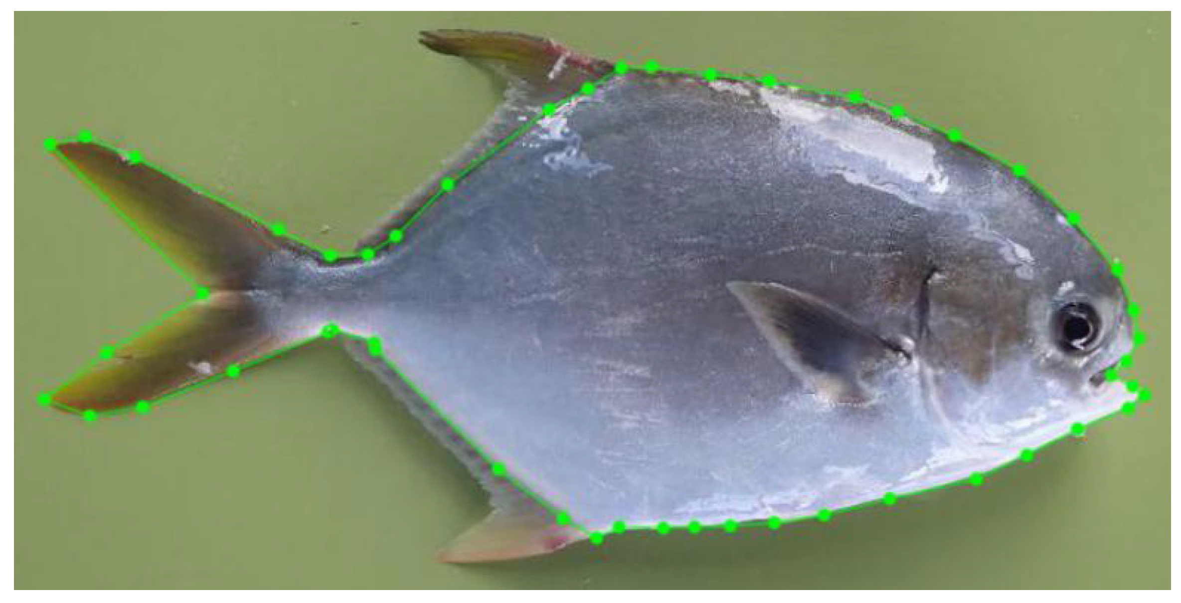
To address the above challenges, we propose a scheme of segmenting and measuring the features of inclined fish using a U-net with increased receptive field in the actual shooting environment. This scheme can realize automatic, batch and high precision segmentation of horizontal and inclined fish, and accurately obtain their BL, BW and area, as shown in Figure 1, In order to better display the experimental results, the detected area is cropped and some obvious segmentation differences are presented with blue frames. The contributions of this paper are as follows.

• The operation of contrast transformation and rotation are used to simulate the actual shooting environment, and a large number of training samples are generated for training by appropriate translation and scaling transformations;
• According to the characteristics of the experimental dataset, the U-net network structure is improved by using a 3 × 3 dilated convolution with a dilation rate 2 and a 1 × 1 convolution to partially replace the 3 × 3 convolution in the original network, the partial convolution receptive field can be expanded to achieve a more accurate segmentation effect;
• Combined with the characteristics of fish body shape, the least squares line fitting method is adopted. The solution realizes accurate measurement of the BL and BW of the inclined fish.

The remainder of this paper is organized as follows: Section 2 briefly introduces the data acquisition and the scheme proposed in this article. Section 3 gives a detailed introduction to the process of data augmentation, improvement of U-net network structure, and least squares line fitting to obtain BL and width. Section 4 describes the process of the experiment in detail and analyzes the results of the experiment. Section 5 summarizes this paper and discusses future directions. The main abbreviations and symbols used are listed in

Table 1. Abbreviations and symbols.

Abbreviations and Symbols	Initial Explanation
mIoU	Mean Intersection over Union
IoU	Intersection over Union
BL	Body Length
BW	Body Width
BA	Body Area
YOLO	You Only Look Once
F	Receptive field
$Ou{t}_{feature}$	Output feature size
$I{n}_{feature}$	Input feature size

.

2. Materials and Brief Description of Proposed Method

2.1. Data Acquisition

Currently, there are few publicly available large-scale fish image datasets. The samples of oval squid (Latin name: Trachinotus ovatus) used in the experiment were collected from the carp farm in Hainan Lingshui Autonomous County, China (Hainan University Marine College Aquaculture Professional Production and Research Base). There are 350 original experimental images, of which 300 are used as the training set and 50 are used as the test set. The fish are placed close to the level to take pictures. The resolution of the collected images is 4608 × 3456. Considering that the excessive resolution leads to a sharp increase in the hardware configuration required for network training. In the experiment, the length and width are reduced by 4 times to 1152 × 684.

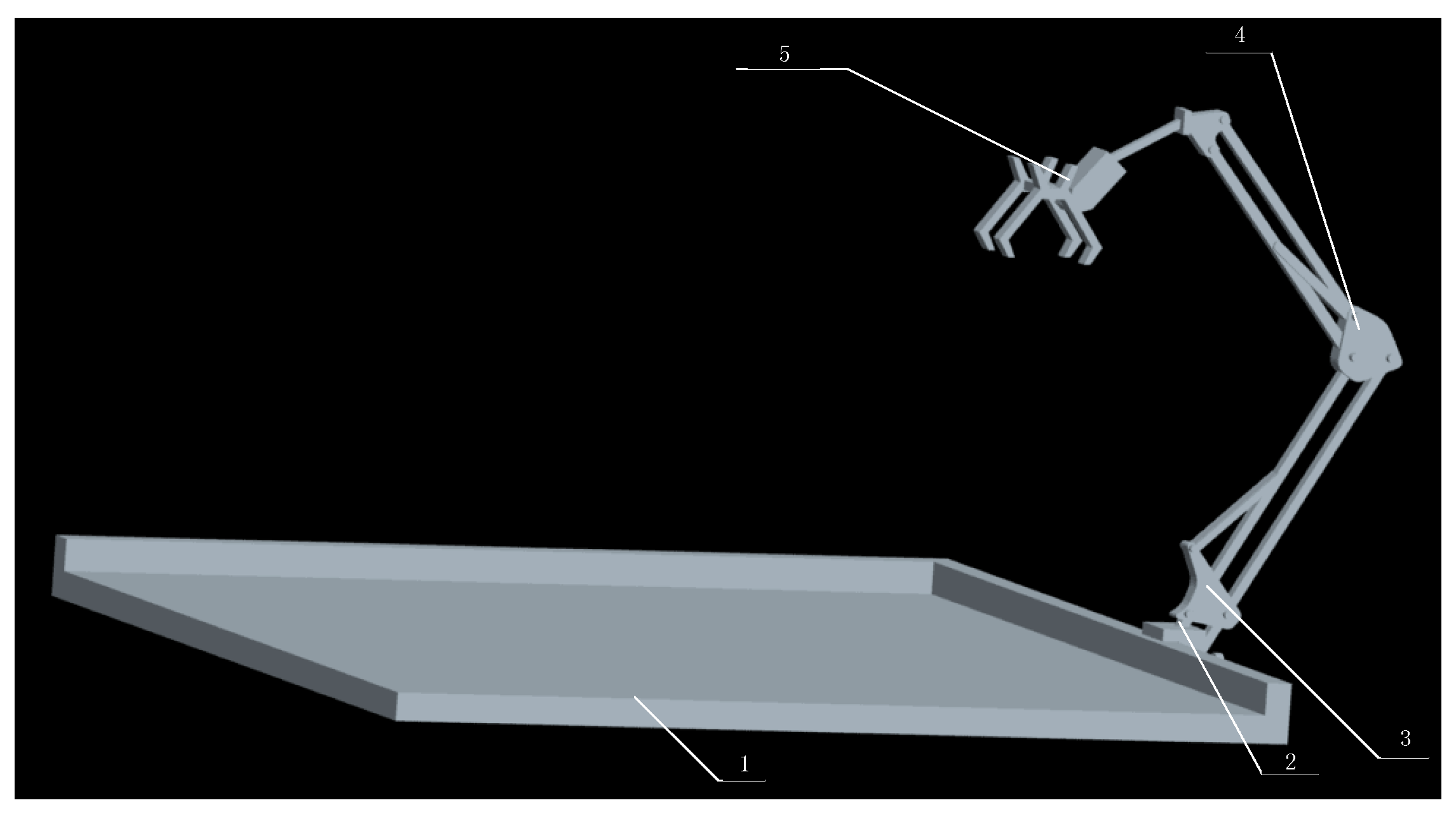
In order to achieve fast, accurate and stable acquisition of fish images, this paper uses a home-made image acquisition device [20]. As shown in Figure 2, the device consists of a standard measuring plate (bottom length 560 mm, width 400 mm) and a mechanical arm. The process of collecting the fish body image is as follows. First, the acquisition camera (OLYMPUS TG-4, f/2.0, focal length: 4 mm, self-contained lens distortion correction) is installed at the end of the execution of the mechanical arm, and then connects it to the computer via a data cable. Next, the position of the camera is set by adjusting the robot arm so that the photographing screen can cover the bottom length of the platform, and the camera lens is parallel to the platform. Finally, we place the fish on the measuring plate and keep the camera directly over the fish body, quickly capture the image, collect the image data of the fish body, and then transmit it to the computer through the data cable.

2.2. Proposed Scheme

The gray-filled modules in Figure 3 are the main work of this paper. From Figure 3, the flow chart is proposed for the segmentation and measurement of inclined fish features by U-net with increased receptive field. First, the original image is acquired through the image acquisition device. Due to the ideal environment when the image is collected, the contrast of the image does not change significantly and the fish body is placed nearly horizontally. In order to better simulate the actual environment, contrast transformation, rotation transformation, translation transformation and scaling transformation are performed on the training set, and contrast transformation and rotation transformation are performed on the test set. The main purpose of the translation and scaling transformations on the training set is to generate more training samples. Second, the expanded training set is input to the improved U-net network for training, and a trained model is obtained. Then, the test samples after image processing are input into the trained model to obtain the accurately segmented binary images [21]. Next, the outer contour acquisition and linear fitting operation based on the least square are performed to obtain the set of contour points of the fish and the fitted line [22,23,24]. Subsequently, the values of BL and BW are obtained by mathematical derivation. Finally, comparing the obtained data with the actual morphological data and the binary image labeled on the test set, we can obtain various indicators for evaluating the performance of the scheme.

3. Detailed Description of Proposed Measurement Method

3.1. Data Augmentation

In order to better simulate the actual processing environment and generate more images for deep learning network learning, data augmentation [25,26,27] is adopted to address the issue of small dataset. The contrast transformation [28] and the rotation transformation are used to simulate the change of light and the incomplete horizontal phenomenon of fish in actual processing, respectively. In the meantime, the translation transformation and the scaling transformation are used to simulate positional differences in the image where the fish is located and individual differences in the fish, respectively.

3.1.1. Contrast Transformation

Contrast transformation is an image processing method that changes the contrast of image pixels by changing the brightness value of image pixels, thereby improving the image quality. In the experiment, the contrast transformation is used to simulate the light transformation in the actual environment. Figure 4 shows the effect of contrast transformation. The value of the contrast transformation used in the experiment is set randomly in the interval of [0.5, 1.5].

3.1.2. Rotation Transformation

Rotation transformation is a transformation that rotates the image and fills the vacant part after rotation with adjacent values. The rotation transformation of the fish is used to simulate the phenomenon that the fish is not level in the actual processing environment. Figure 5 shows the effect of rotation transformation. The value of the rotation transformation used in this experiment is set randomly in the interval of [−45°, 45°].

3.1.3. Translation Transformation

Translation transformation is to translate the image horizontally and vertically, but the resolution of the image is unchanged. For the vacant part after translation, adjacent values will be used for padding. The translation transformation can be used to solve the differences in the position of the fish in the image and to produce a large number of training images. In order to better display the translation effect, a slightly larger translation ratio column is selected for presentation, and the transformation effect is shown in Figure 6. In the experiment, the ratio of horizontal or vertical translation length to picture length is within [0, 0.02].

3.1.4. Scaling Transformation

Scaling transformation randomly scales the length and width of the image, but the resolution of the image does not change. The enlarged image is intercepted and the reduced image is filled with neighboring values. The scaling transformation can be used to generate a large number of samples of different fish sizes for the network to learn from. In order to better display the scaling effect, a slightly larger scaling ratio is used for presentation. Figure 7 shows the effect of scaling transformation. In the experiment, the ratio of scaling transformation to the image is within [0, 0.01].

3.2. Improved U-Net Network Structure

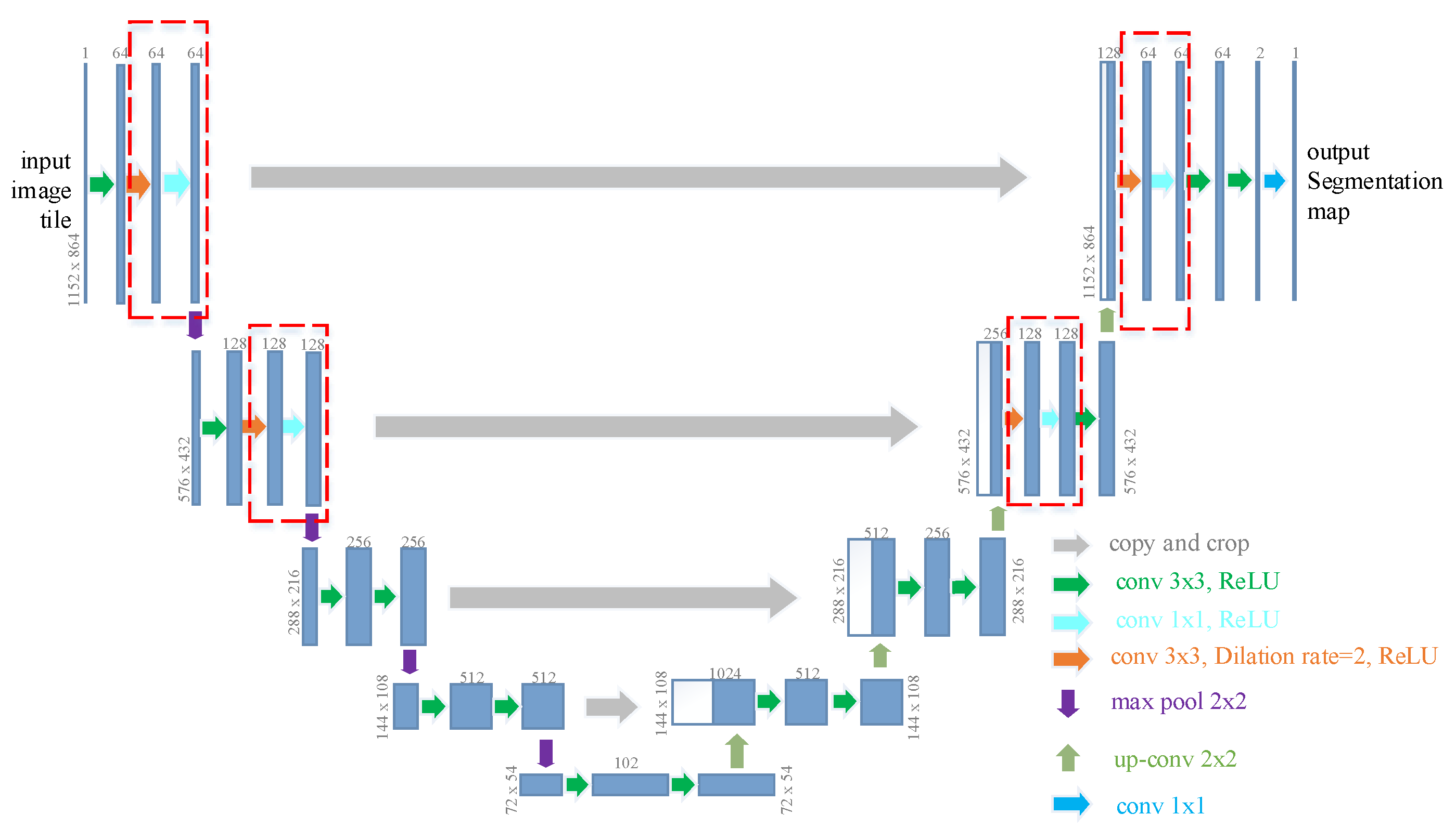
U-net [29] is a classic network for segmentation tasks [30], which adopts the encoder-decoder structure and channel dimension splicing to integrate the multi-scale features [31]. The network is widely used due to its advantage, supporting a small amount of data to train the model, simple structure, high segmentation accuracy and fast segmentation speed. According to the characteristics of the experimental data set as well as the large proportion of fish in the image, the U-net network structure is improved to provide a larger receptive field for the partial convolution. The improved U-net uses a 3 × 3 dilated convolution [32,33,34] with a dilation rate of 2 and one 1 × 1 convolution to partially replace the 3 × 3 convolution in the original network. The partial replacement is to avoid too many dilated convolution leading to gridding effect [35].

The improved U-net network is shown in Figure 8, in which the red virtual box is the main part of the improvement.

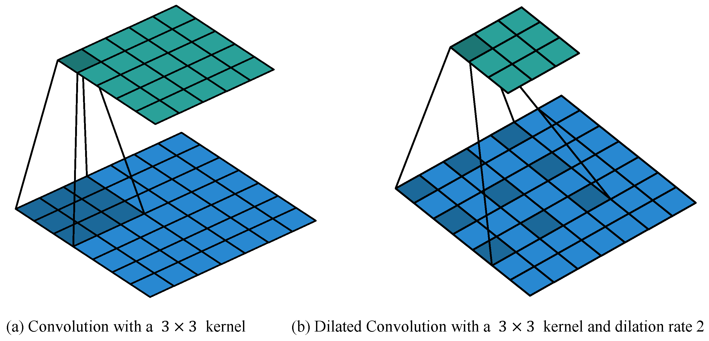
The role of dilated convolution in the improved U-net structure is to expand the receptive field [36]. The schematic diagram of its work is shown in Figure 9b. In Figure 9, the stride of convolution is 1 and no padding operation is performed. It can be seen from Figure 9 that by using dilated convolution with a 3 × 3 kernel and a dilation rate of 2, the receptive field of each convolution is amplified from 3 × 3 to 5 × 5. In this way, each convolution output contains a large range of information of the original feature map, and appropriately compensates for some feature loss caused by the pooling operation in the U-net network [37].

For the dilated convolution, calculation formula of receptive field is:

$$F=(2\times dilation-1)\times (kernel-1)+kernel;$$

(1)

and the calculation formula of output feature size is:

$$ou{t}_{feature}=\frac{i{n}_{feature}-F+2\times padding}{stride}+1.$$

(2)

Figure 10a shows the working diagram of a 1 × 1 convolution when both input and output channels are 1, where the value in the filter is the weight value to be learned. Figure 10b shows the working diagram for input channels with N and output channel as 1. Therefore, 1 × 1 convolution in the improved U-net network is equivalent to adding an auto-learnable coefficient on the basis of each dilated convolution, and then combining multi-dimensional information [38]. This operation has the effect of enhancing cross-group information exchange and non-linearity, thereby achieving a certain degree of adaptive optimization and adjustment effect on the features collected after expanding the receptive field [39,40].

3.3. Line Fitting Scheme

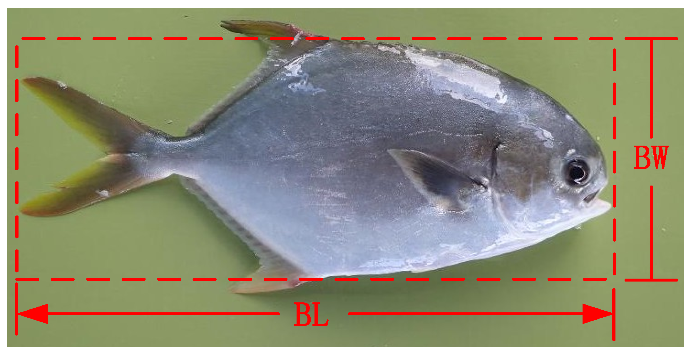
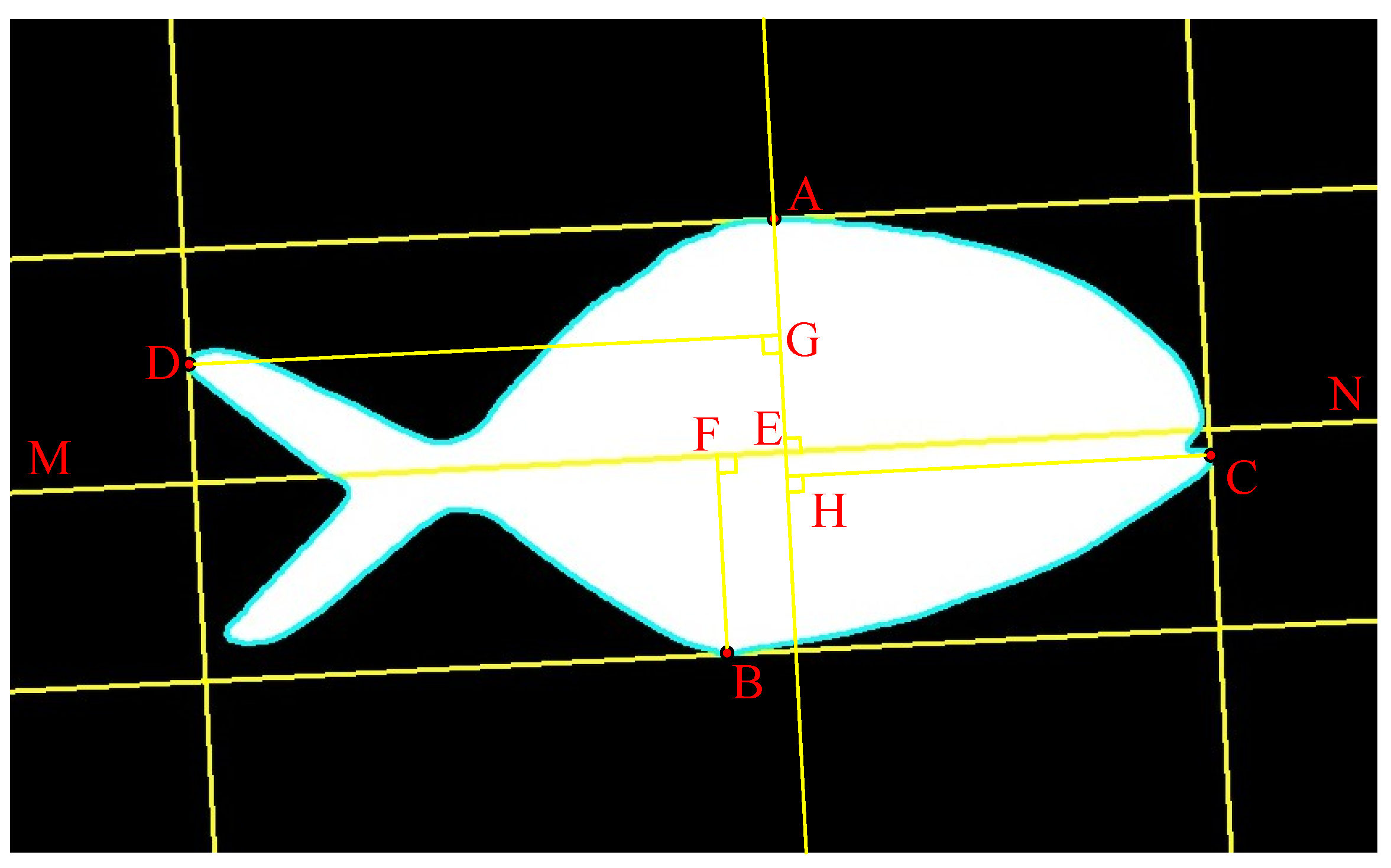
Figure 11 and Figure 12 show the measurement range standards for the corresponding characteristics after the actual requirements are known [41]. In Figure 11, BL and BW represent the BL and the BW of the fish, respectively. In Figure 12, the area surrounded by green dots and lines is the required fish area.

In Figure 11 and Figure 12, the fish bodies are all in a horizontal state. When the fish bodies are no longer close to the horizontal state, an accurately judge the angle of the fish inclination becomes a challenge. By combining the characteristics of the fish body shape and the improved U-net to obtain a precise binary segmentation image, the idea of microscopicizing the fish body into multiple pixels is proposed. The least squares method [42,43] is used to fit the point set in a straight line, and the angle of the straight line can be regarded as the angle of the fish. At the same time, the method also conforms to the judgment logic of human judging the tilt direction of fish.

Figure 13 shows a working diagram of the body length and width of the inclined fish calculated by combining the outer contour detection of fish and line fitting. All the intersecting lines in Figure 13 are vertical. First, the contour point set of the segmented binary image is obtained by using outer contour detection, and the linear equation of MN (y = kx + b) was obtained by using the line fitting. Second, the contour point set

$$Q=\left[\left(x_1,y_1\right),\left(x_2,y_2\right),\left(x_3,y_3\right),\cdots ,\left(x_n,y_n\right)\right]$$

(3)

is divided into two parts by the straight line of MN. For each point set, the shortest distance d from each point to line MN was calculated [44],

$$d=\frac{\left|{kx}_i=y_i+b\right|}{\sqrt{k^2+1}}$$

(4)

and the longest distance of all distances (AE, BF) and the point that reached the longest distance (point A, point B) were selected. The length of the line segments AE($l_1$) and BF($l_2$) is the BW of the fish.

$$\mathrm{BW}=l_1\pm l_2.$$

(5)

Then, since the line AE is perpendicular to MN, the slope of the line AE ($k_1$ = $-\frac{1}{k}$) is obtained according to the slope of the line MN. Based on the known coordinates of point A, the equation of the straight line AE (y = $k_1$x + $b_1$) can be obtained. Next, taking the same operation as above, the straight line AE divides the contour point set into two parts. The coordinates of the points C and D and the lengths of the line segments CH ($l_3$) and DG ($l_4$) are obtained, respectively. The sum of the lengths of the line segments CH and DG is the BL of the fish.

$$\mathrm{BL}=l_3\pm l_4.$$

(6)

Finally, four straight lines are drawn according to the known points A, B, C, D and the corresponding slope of the tangent line for a more intuitive display. The pseudo code description of the line fitting scheme is shown in Algorithm 1.

Algorithm 1 Pseudo code description of the line fitting scheme.

Input:$ContourpointsetisQ=\left[\left(x_1,y_1\right),\left(x_2,y_2\right),\cdots ,\left(x_i,y_i\right),\cdots ,\left(x_n,y_n\right)\right];$   Fitting Linear MN Equation by Least Square Method is $y=kx+b$. Output:$body\_width,body\_length,\alpha$.   $Algorithmflow$:    Step 1: Obtain the body_width. 1: forI in Q do 2:     if $\left(I\right[1]>kl[0]+b)$ then 3:         $\mathrm{dis}=\frac{\left|\mathrm{kl}\right[0]+b-I[1\left]\right|}{\sqrt{k^2+1}};$ #Shortest distance from point to straight line 4:          5:         if $\mathbf{then} \left(l_1<=\mathrm{dis}\right);$ 6:              $l_1=\mathrm{dis};$ 7:              $A=\left(I\right[0],I[1\left]\right)$; 8:         else 9:              $\mathrm{continue};$ 10:         end if 11:     else 12:         $\mathrm{Follow}\mathrm{the}\mathrm{steps}\mathrm{above}\mathrm{to}\mathrm{find}\mathrm{the}\mathrm{length}\mathrm{of}{l}_2\mathrm{and}\mathrm{the}\mathrm{coordinates}\mathrm{of}\mathrm{point}\mathrm{B};$ 13:     end if 14: end for $BW=l_1+l_2$. Step 2: Obtain the body_length. Pass point A to make AE perpendicular to MN, and drop foot   to point E; $Let{k}_1=-\frac{1}{k},b_1=\frac{I\left[1\right]+I\left[0\right]}{k};theequationofthestraightlineAE:y=k_{1}x+b_1$ 15: forJ in Q do 16:     if $(J\left[0\right]>\frac{J\left[1\right]-b_1}{k_1})$ then 17:         $\mathrm{dis}=\frac{\mid kJ\left[0\right]+b_1-J1]\mid }{\sqrt{k_1^2+1}};$ 18:          19:         if $\mathbf{then} \left(l_3<=\mathrm{dis}\right);$ 20:              $l_3=\mathrm{dis};$ 21:              $C=\left(J\right[0],J[1\left]\right)$; 22:         else 23:              $\mathrm{continue};$ 24:         end if 25:     else 26:         $\mathrm{Follow}\mathrm{the}\mathrm{steps}\mathrm{above}\mathrm{to}\mathrm{find}\mathrm{the}\mathrm{length}\mathrm{of}{l}_4\mathrm{and}\mathrm{the}\mathrm{coordinates}\mathrm{of}\mathrm{point}\mathrm{D};$ 27:     end if 28: end for $BL=l_3+l_4$. Step 3: Obtain the tile angle. According to point A, pint B, point C, point D and related slopes, the four tangent lines corresponding to the inclined fish can be obtained. Fish tilt angle is   $\alpha =arctank$.

4. Experimental Results and Analysis

4.1. Experimental Environment and Parameter Settings

The experimental environment is the ubuntu18.04.1 operating system, Tesla v100 GPU, keras platform and python3. To ensure the reliability of the experiment and the adequacy of the network training, we set the batch size to 2, the learning rate to 5 × 10${}^{-6}$, the epoch to 50, and the number of iterations per round to 600. For the label of the data set, labelme software [45] is used to obtain the mask image in the experiment. Then the mask image is converted into a binary image in uint8 format to be trained as a labeled image. For the data set and code used in the experiment, please see the link in Supplementary Materials.

4.2. Evaluation Indicators

In the experiment, to evaluate the effect of network segmentation, a better analysis of the network performance and the needs of actual production are considered. mIoU [46], average accuracy rate, average recall rate [47], and average area relative error are used as evaluation indicators. To evaluate the measurement of BL and BW of fish, the average relative error is used as the evaluation indicator.

4.3. Improved U-Net Performance Verification

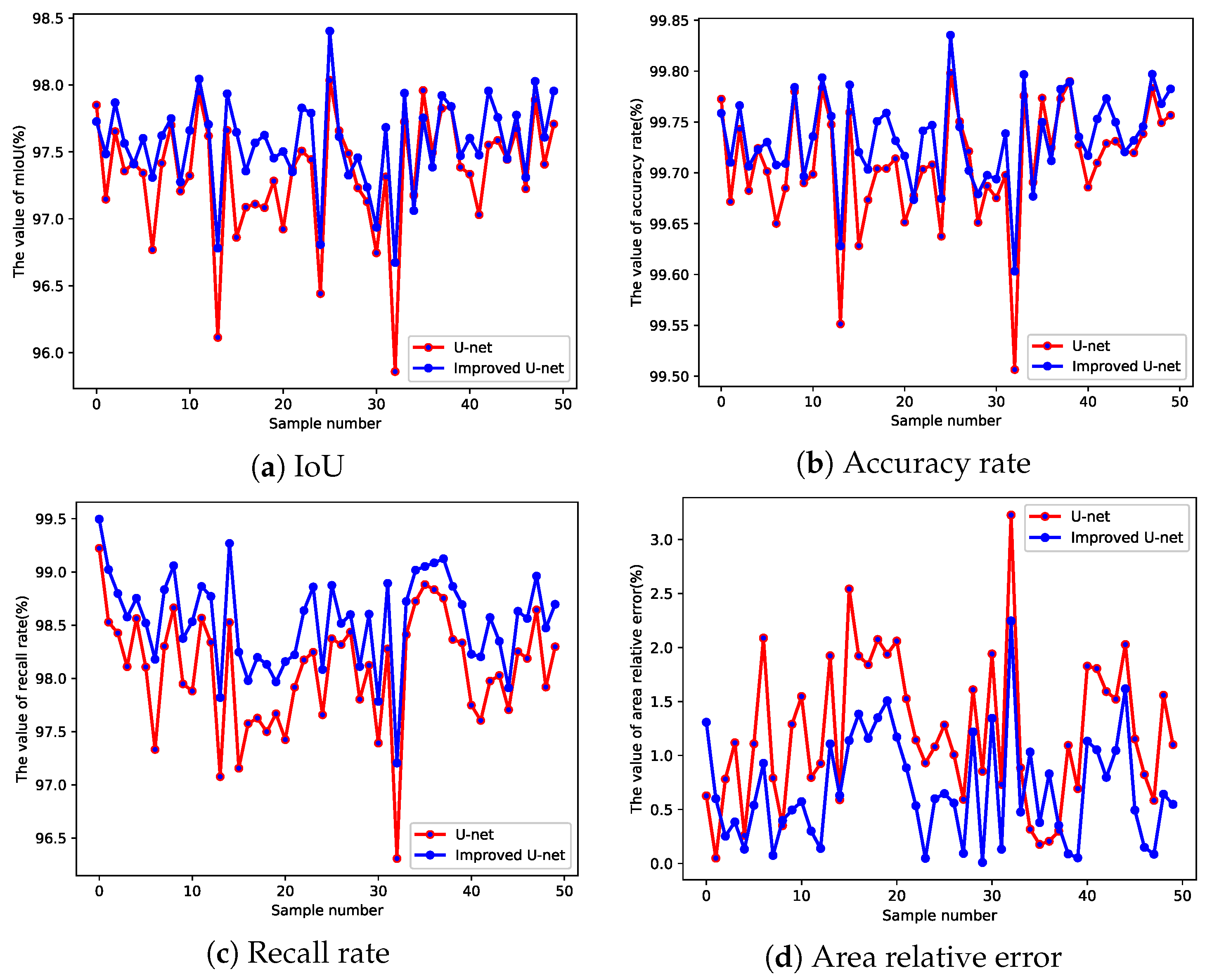
In order to initially verify the performance of the improved U-net network structure, no rotation transformation is performed on the original data set. The line chart of IoU, accuracy rate, recall rate and area relative error of 50 test images by two networks is shown in Figure 14.

From

Table 2. Numerical comparison of two networks on four metrics when the fish are placed horizontally.

Indicators	mIoU (%)	Average Accuracy Rate (%)	Average Recall Rate (%)	Average Area Relative Error (%)
U-net	97.56	99.73	98.14	1.29
Improved U-net	97.66	99.74	98.55	0.72

, the results of mIoU, average accuracy rate, average recall rate and average area relative error are calculated. It can be seen from the data that the improved network is better than that of U-net in terms of performance, and the average relative error is reduced to about a half.

4.4. Feature Measurement for Tilted Fish

To simulate the actual production environment, the fish may be tilted when placed on a conveyor belt or on a fish measuring plate. The environment is simulated by randomly rotating the training and test sets within an angle of [−45°, 45°]. To further verify the applicability of the improved U-net network, two models are generated using original and improved network training, and 50 test images are tested. The experimental results of segmentation by using U-net and improved U-net are shown in Figure 15, where the detected area is cropped and some obvious segmentation differences are represented by blue frames for better display.

From Figure 15, the improved U-net has a better segmentation effect on the edge of the fish, and the improved U-net can accurately segment the requested inclined fish BA. The line chart of IoU, accuracy rate, recall rate and area relative error of 50 test images by two networks is shown in Figure 16.

As shown in

Table 3. Numerical comparison of two networks on four metrics when the fish are tilted.

Indicators	mIoU (%)	Average Accuracy Rate (%)	Average Recall Rate (%)	Average Area Relative Error (%)
U-net	97.35	99.71	98.08	1.20
Improved U-net	97.57	99.73	98.54	0.69

, the results of mIoU, average accuracy rate, average recall rate and average area relative error are calculated. According to the data in Table 3, the improved U-net is still better than U-net with mIoU as high as 97.6%. Compared with U-net, the average relative error of the area is still reduced to about a half.

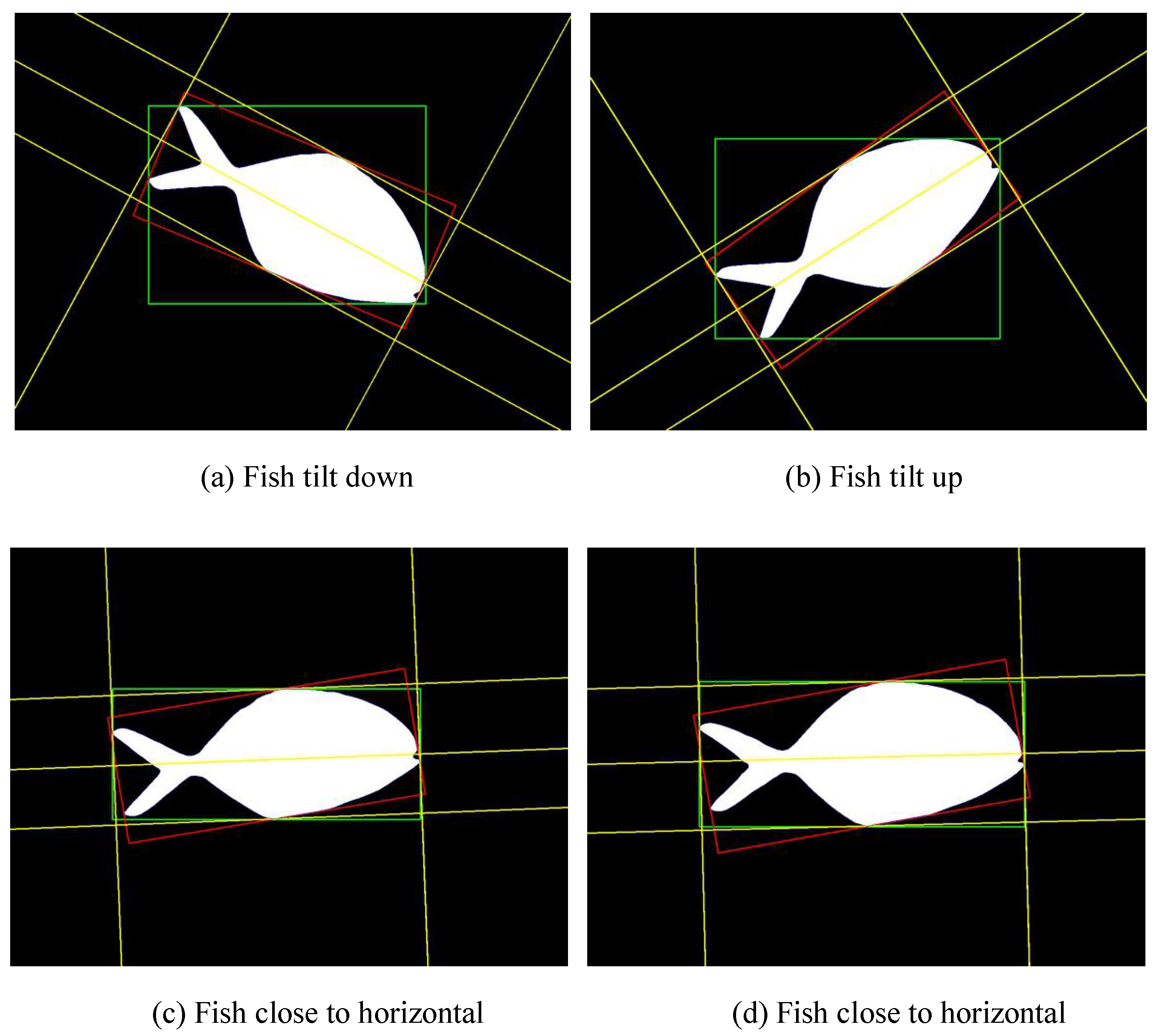
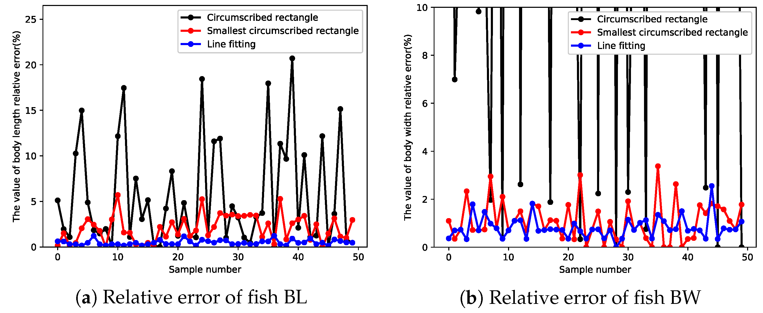
To measure fish BL and BW, the line fitting scheme in this paper is also compared with the commonly used circumscribed rectangle [48] and the smallest circumscribed rectangle [49] method in the experiment. In order to ensure the accuracy of the experiment, the true length and width of the test fish are expressed by the number of pixels in the picture occupied by the BL and BW. The average value of three manual measurements is used as the standard value. The test result images are shown in Figure 17.

As shown in Figure 17, the yellow line represents the result of the line fitting scheme, the red box represents the result of the smallest circumscribed rectangle scheme, and the green box represents the result of using the circumscribed rectangle scheme. From Figure 17c,d, when the fish is close to horizontal, the smallest circumscribed rectangle is still inclined at a certain angle. This will lead to a large error.

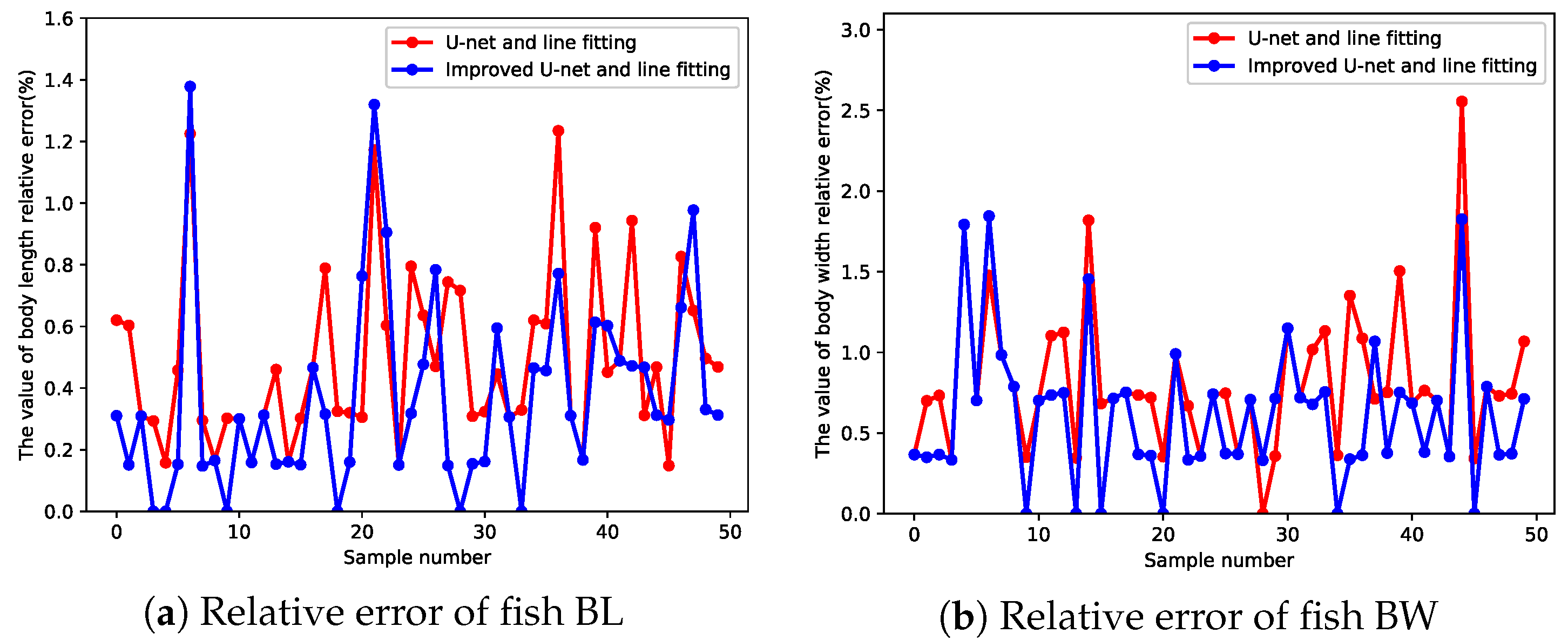
To observe the performance differences in measurement by using different measurement schemes more intuitively, line charts are drawn with the relative error as the indicator. From Figure 18, Figure 19 and Figure 20, the line fitting scheme proposed in this paper is superior to the circumscribed rectangle and the smallest circumscribed rectangle. The improved U-net network is better than the previous network.

It can be seen from

Table 4. Average relative errors of various schemes.

Schemes	U-net		Improved U-net
	Average Relative Error of BL (%)	Average Relative Error of BW (%)	Average Relative Error of BL (%)	Average Relative Error of BW (%)
Circumscribed rectangle	5.56	39.91	5.56	40.08
Smallest circumscribed rectangle	2.07	1.09	1.99	1.07
Line fitting	0.49	0.81	0.37	0.61

that the comprehensive scheme of improved U-net and line fitting can accurately measure the BL and BW of inclined fish. At this time, the relative errors of BL and BW are 0.37% and 0.61%, respectively. Because the line fitting method is used, the specific tilt angle of the fish body can be obtained from the slope of the fitted straight line. The angle parameter is also of great significance for object grabbing [50].

5. Conclusions and Future Work

Obviously, the accurately measured morphological characteristic data can be used as an important reference for feeding, fishing, classification and genetic breeding in aquaculture research. This paper proposes an accurate method for measuring the actual size for the length, width and area of the fish body. This method is especially effective for measuring the characteristics of the fish body in a tilted state. The proposed method mainly includes a data set expansion module, a segmentation module using improved U-net model, and the least square linear fitting module, which can achieve the segmentation of a tilted fish body in the images and accurate measurement of various characteristics. The experimental comparison results of various metrics show that the performance of the measurement system is indeed improved. Specifically, the mIoU of the improved U-net model can reach 97.6%. The average relative error of the fish BA can be reduced to 0.69%. The average relative error of the BL and width can be reduced to 0.37% and 0.61%, respectively. In conclusion, the proposed method can achieve the purpose of accurate measurement of fish body morphological characteristics in practical applications. In addition, the inclination angle of the fish body obtained in the calculation process can also be used as a useful parameter for realizing the automatic capture of the fish.

The research of this paper divides the fish body segmentation, the pixel size calculation, and the conversion from pixel size to actual size into three different steps. In our future research, we will consider combining segmentation, pixel size prediction and actual size conversion into one network model in one step. This can greatly improve the efficiency of the measurement process.

References

1. Antonio, S.; Rodolfo, P.; del Giudice, A.; Francesco, L.; Paolo, M.; Enrico, S.; Alberto, A. Semi-Automatic Guidance vs. Manual Guidance in Agriculture: A Comparison of Work Performance in Wheat Sowing. Electronics 2021, 10, 825. [Google Scholar]
2. Ania, C.; Samuel, S. Use and Adaptations of Machine Learning in Big Data—Applications in Real Cases in Agriculture. Electronics 2021, 10, 552. [Google Scholar]
3. Hu, Z.H.; Zhang, Y.R.; Zhao, Y.C.; Xie, M.S.; Zhong, J.Z.; Tu, Z.G.; Liu, J.T. A Water Quality Prediction Method Based on the Deep LSTM Network Considering Correlation in Smart Mariculture. Sensors 2019, 19, 1420. [Google Scholar] [CrossRef] [PubMed] [Green Version]
4. Liu, J.T.; Yu, C.; Hu, Z.H.; Zhao, Y.C.; Bai, Y.; Xie, M.S.; Luo, J. Accurate Prediction Scheme of Water Quality in Smart Mariculture With Deep Bi-S-SRU Learning Network. IEEE Access 2020, 8, 24784–24798. [Google Scholar] [CrossRef]
5. Li, D.L.; Liu, C. Recent advances and future outlook for artificial intelligence in aquaculture. Smart Agric. 2020, 2, 1–20. [Google Scholar]
6. Hu, Z.H.; Li, R.Q.; Xia, X.; Yu, C.; Fan, X.; Zhao, Y.C. A method overview in smart aquaculture. Environ. Monit. Assess. 2020, 192, 1–25. [Google Scholar] [CrossRef]
7. Wageeh, Y.; Mohamed, H.E.D.; Fadl, A.; Anas1, O.; ElMasry, N.; Nabil, A.; Atia, A. YOLO fish detection with Euclidean tracking in fish farms. J. Ambient. Intell. Humaniz. Comput. 2021, 12, 5–12. [Google Scholar] [CrossRef]
8. Hu, J.; Zhao, D.; Zhang, Y.; Zhou, C.; Chen, W. Real-time nondestructive fish behavior detecting in mixed polyculture system using deep-learning and low-cost devices. Expert Syst. Appl. 2021, 178, 115051. [Google Scholar] [CrossRef]
9. Wu, H.; He, S.; Deng, Z.; Kou, L.; Huang, K.; Suo, F.; Cao, Z. Fishery monitoring system with AUV based on YOLO and SGBM. In Proceedings of the 2019 Chinese Control Conference (CCC), Guangzhou, China, 27–30 July 2019; pp. 4726–4731. [Google Scholar]
10. Liu, S.; Li, X.; Gao, M.; Cai, Y.; Rui, N.; Li, P.; Yan, T.; Lendasse, A. Embedded online fish detection and tracking system via YOLOv3 and parallel correlation filter. In Proceedings of the OCEANS 2018 MTS/IEEE Charleston, Charleston, SC, USA, 22–25 October 2018; pp. 1–6. [Google Scholar]
11. Hao, M.M.; Yu, H.L.; Li, D.L. The measurement of fish size by machine vision—A review. IFIP Adv. Inf. Commun. Technol. 2016, 479, 15–32. [Google Scholar]
12. An, A.Q.; Yu, Z.T.; Wang, H.Q.; Nie, Y.F. Application of machine vision technology in agricultural machinery. J. Anhui Agric. Sci. 2007, 12, 3748–3749. [Google Scholar]
13. Yu, X.J.; Wu, X.F.; Wang, J.P.; Chen, L.; Wang, L. Rapid Detecting Method for Pseudosciaena Crocea Morphological Parameters Based on the Machine Vision. J. Integr. Technol. 2014, 3, 45–51. [Google Scholar]
14. Hu, Z.H.; Zhang, Y.R.; Zhao, Y.C.; Cao, L.; Bai, Y.; Huang, M.X. Fish eye recognition based on weighted constraint AdaBoost and pupil diameter automatic measurement with improved Hough circle transform. Trans. Chin. Soc. Agric. Eng. 2017, 33, 226–232. [Google Scholar]
15. Hu, Z.H.; Cao, L.; Zhang, Y.R.; Zhao, Y.C. Study on fish caudal peduncle measuring method based on image processing and linear fitting. Fish. Mod. 2017, 44, 43–49. [Google Scholar]
16. Yao, H.; Duan, Q.L.; Li, D.L.; Wang, J.P. An improved K-means clustering algorithm for fish image segmentation. Math. Comput. Model. 2013, 58, 790–798. [Google Scholar] [CrossRef]
17. Cook, D.; Middlemiss, K.; Jaksons, P.; Davison, W.; Jerrett, A. Validation of fish length estimations from a high frequency multi-beam sonar (ARIS) and its utilisation as a field-based measurement technique. Fish. Res. 2019, 218, 59–68. [Google Scholar] [CrossRef]
18. Yu, C.; Fan, X.; Hu, Z.H.; Xia, X.; Zhao, Y.C.; Li, R.Q.; Bai, Y. Segmentation and measurement scheme for fish morphological features based on Mask R-CNN. Inf. Process. Agric. 2020, 7, 523–534. [Google Scholar] [CrossRef]
19. Tseng, C.H.; Hsieh, C.L.; Kuo, Y.F. Automatic measurement of the body length of harvested fish using convolutional neural networks. Biosyst. Eng. Inf. Process. Agric. 2020, 189, 36–47. [Google Scholar] [CrossRef]
20. Hu, Z.H.; Cao, L.; Zhang, Y.R.; Zhao, Y.C.; Huang, M.X.; Xie, M.S. Study on eye feature detection method of Trachinotus ovatus based on computer vision. Fish. Mod. 2017, 44, 15–23. [Google Scholar]
21. He, L.F.; Ren, X.W.; Zhao, X.; Yao, B.; Kasuya, H.; Chao, Y.Y. An efficient two-scan algorithm for computing basic shape features of objects in a binary image. J. Real Time Image Process. 2019, 16, 1277–1287. [Google Scholar] [CrossRef]
22. Xu, S.Y.; Peng, C.L.; Chen, K.; Wang, L.Q.; Ren, X.F.; Duan, H.B. Measurement Method of Wheat Stalks Cross Section Parameters Based on Sector Ring Region Image Segmentation. Nongye Jixie Xuebao/Trans. Chin. Soc. Agric. Mach. 2018, 49, 53–59. [Google Scholar]
23. Arbeláez, P.; Maire, M.; Fowlkes, C.; Malik, J. Contour Detection and Hierarchical Image Segmentation. IEEE Trans. Pattern Anal. Mach. Intell. 2011, 33, 898–916. [Google Scholar] [CrossRef] [Green Version]
24. Petkovic, T.; Lonc aric, S. Using Gradient Orientation to Improve Least Squares Line Fitting. In Proceedings of the 2014 Canadian Conference on Computer and Robot Vision, Montreal, QC, Canada, 6–9 May 2014; pp. 226–231. [Google Scholar]
25. Fu, Y.; Li, X.T.; Ye, Y.M. A multi-task learning model with adversarial data augmentation for classification of fine-grained images. Neurocomputing 2020, 377, 122–129. [Google Scholar] [CrossRef]
26. Pandey, P.; Dewangan, K.K.; Dewangan, D.K. Enhancing the quality of satellite images by preprocessing and contrast enhancement. In Proceedings of the 2017 International Conference on Communication and Signal Processing (ICCSP), Melmaruvathur, India, 6–8 April 2017; pp. 56–60. [Google Scholar]
27. Zhu, Q.Y.; Li, T.T. Semi-supervised learning method based on predefined evenly-distributed class centroids. Appl. Intell. 2020. [Google Scholar] [CrossRef] [Green Version]
28. Matsumoto, M. Cognition-based contrast adjustment using neural network based face recognition system. In Proceedings of the 2010 IEEE International Symposium on Industrial Electronics, Bari, Italy, 4–7 July 2010; pp. 3590–3594. [Google Scholar]
29. Ronneberger, O.; Fischer, P.; Brox, T. U-Net: Convolutional networks for biomedical image segmentation. In Proceedings of the Medical Image Computing and Computer-Assisted Intervention—MICCAI, Munich, Germany, 5–9 October 2015; pp. 234–241. [Google Scholar]
30. Shelhamer, E.; Long, J.; Darrell, T. Fully Convolutional Networks for Semantic Segmentation. IEEE Trans. Pattern Anal. Mach. Intell. 2017, 39, 640–651. [Google Scholar] [CrossRef]
31. Wu, Y.P.; Jin, W.D.; Ren, J.X.; Sun, Z. A multi-perspective architecture for high-speed train fault diagnosis based on variational mode decomposition and enhanced?multi-scale structure. Appl. Intell. 2019, 49, 3923–3937. [Google Scholar] [CrossRef]
32. Yu, F.; Koltun, V. Multi-scale context aggregation by dilated convolutions. arXiv 2015, arXiv:1511.07122. [Google Scholar]
33. Chen, L.C.; Zhu, Y.K.; Papandreou, G.; Schroff, F.; Adam, H. Encoder-Decoder with Atrous Separable Convolution for Semantic Image Segmentation. In Proceedings of the Computer Vision—ECCV 2018, Munich, Germany, 8–14 September 2018; pp. 833–851. [Google Scholar]
34. Lin, G.M.; Wu, Q.W.; Qiu, L.D.; Huang, X.X. Image super-resolution using a dilated convolutional neural network. Neurocomputing 2018, 275, 1219–1230. [Google Scholar] [CrossRef]
35. Yu, F.; Koltun, V. Funkhouser T. Dilated residual network. arXiv 2017, arXiv:1705.09914. [Google Scholar]
36. Ma, J.J.; Dai, Y.P.; Tan, Y.P. Atrous convolutions spatial pyramid network for crowd counting and density estimation. Neurocomputing 2019, 350, 91–101. [Google Scholar] [CrossRef]
37. He, K.M.; Gkioxari, G.; Dollár, P.; Girshick, R. Mask R-CNN. arXiv 2018, arXiv:1703.06870. [Google Scholar]
38. Lin, M.; Chen, Q.; Yan, S.C. Network In Network. arXiv 2014, arXiv:1312.4400. [Google Scholar]
39. Szegedy, C.; Liu, W.; Jia, Y.Q.; Sermanet, P.; Reed, S.; Anguelov, D.; Erhan, D.; Vanhoucke, V.; Rabinovich, A. Going Deeper with Convolutions. arXiv 2014, arXiv:1409.4842. [Google Scholar]
40. He, K.M.; Zhang, X.Y.; Ren, S.Q.; Sun, J. Deep residual learning for image recognition. In Proceedings of the the IEEE Computer Society Conference on Computer Vision and Pattern Recognition, Las Vegas, NV, USA, 26–30 June 2016; pp. 770–778. [Google Scholar]
41. Hu, X.L.; Chen, Q.Y.; Shen, J. Study on Morphological characteristics and correlation analysis of trachurus japonicus from southern east china sea. Acta Zootaxonomica Sin. 2013, 38, 407–412. [Google Scholar]
42. Song, S.M.; Wang, M.; Hu, X.W. Data reconstruction for nanosensor by using moving least square method. Process. Autom. Instrum. 2010, 31, 16–18. [Google Scholar]
43. Mir, A.; Nasiri, J.A. KNN-based least squares twin support vector machine for pattern classification. Appl. Intell. 2018, 48, 4551–4564. [Google Scholar] [CrossRef]
44. Hsu, T.S.; Wang, T.C. An improvement stereo vision images processing for object distance measurement. Int. J. Autom. Smart Technol. 2015, 5, 85–90. [Google Scholar]
45. Torralba, A.; Russell, B.C.; Yuen, J. LabelMe: Online Image Annotation and Applications. Proc. IEEE 2010, 98, 1467–1484. [Google Scholar] [CrossRef]
46. Zhuang, H.; Zhuang, H.; Wang, C.; Xie, J. Co-Occurrent Features in Semantic Segmentation. In Proceedings of the 2019 IEEE/CVF Conference on Computer Vision and Pattern Recognition (CVPR), Long Beach, CA, USA, 15–20 June; pp. 548–557.
47. Ma, F. Research on Image Annotation Based on Regional Segmentation; National University of Defense Technology: Changsha, China, 2017. [Google Scholar]
48. Wang, L.Q.; Li, S.P.; Lv, Z.J. Study of tool wear extent monitoring based on contour extraction. Manuf. Technol. Mach. Tool 2019, 11, 94–98. [Google Scholar]
49. Qin, Y.; Na, Q.C.; Liu, F.; Wu, H.B.; Sun, K. Strain gauges position based on machine vision positioning. Integr. Ferroelectr. 2019, 200, 191–198. [Google Scholar] [CrossRef]
50. Xiao, S.G. Position and Attitude Determination Based on Deep Learning for Object Grasping; Harbin Engineering University: Harbin, China, 2019. [Google Scholar]
Figure 1. Comparison of segmentation results using U-net and improved U-net, respectively. (a) Original image; (b) The segmentation effect on the edge of the fish using U-net; (c) The segmentation effect using the improved U-net. Obviously, the latter has a better effect.
Electronics 10 01426 g001
Figure 2. Image acquisition device. “1” is the standard measuring plate, “2” is the fixing clamp, “3” is the knob, “4” is the mechanical arm, and “5” is the end-effector.
Electronics 10 01426 g002
Figure 3. The system flow chart of the proposed measurement method.
Electronics 10 01426 g003
Figure 4. Data augmentation by contrast transformation.
Electronics 10 01426 g004
Figure 5. Data augmentation by rotation transformation.
Electronics 10 01426 g005
Figure 6. Data augmentation by translation transformation.
Electronics 10 01426 g006
Figure 7. Data augmentation by scaling transformation.
Electronics 10 01426 g007
Figure 8. Structure of improved U-net model.
Electronics 10 01426 g008
Figure 9. Working diagram of ordinary convolution and dilated convolution.
Electronics 10 01426 g009
Figure 10. Working diagram of 1 × 1 convolution operation.
Electronics 10 01426 g010
Figure 11. Measurement standards of fish BL and BW.
Electronics 10 01426 g011
Figure 12. Measurement standard of fish BA.
Electronics 10 01426 g012
Figure 13. Working diagram of contour detection and line fitting.
Electronics 10 01426 g013
Figure 14. Comparison of performance on four metrics when the fish body is not tilted.
Electronics 10 01426 g014
Figure 15. Comparison of segmentation effects of two algorithms when the fish body is tilted.
Electronics 10 01426 g015
Figure 16. Comparison of performance on four metrics when the fish body is tilted.
Electronics 10 01426 g016
Figure 17. Comparison of the effects of three measurement methods. Circumscribed rectangle is marked with a green line; Smallest circumscribed rectangle is marked with a red line; Line fitting rectangle is marked with a yellow line.
Electronics 10 01426 g017
Figure 18. Comparison of relative measurement errors using U-net combined with three measurement methods.
Electronics 10 01426 g018
Figure 19. Comparison of relative measurement errors using improved U-net combined with three measurement methods.
Electronics 10 01426 g019
Figure 20. Comparison of relative measurement errors using two networks combined with line fitting.
Electronics 10 01426 g020