Article

Multiple Instance Learning with Differential Evolutionary Pooling

1
Department of Applied Science & Engineering, Indian Institute of Technology Roorkee, Roorkee 247667, India
2
AI Graduate School, Gwangju Institute of Science & Technology, Gwangju 61005, Korea
3
Department of Computer Science, Korea National Open University, Seoul 03087, Korea
*
Author to whom correspondence should be addressed.
Electronics 2021, 10(12), 1403; https://doi.org/10.3390/electronics10121403
Submission received: 31 March 2021 / Revised: 3 June 2021 / Accepted: 9 June 2021 / Published: 10 June 2021

Abstract

:
While implementing Multiple Instance Learning (MIL) through Deep Neural Networks, the most important task is to design the bag-level pooling function that defines the instance-to-bag relationship and eventually determines the class label of a bag. In this article, Differential Evolutionary (DE) pooling—an MIL pooling function based on Differential Evolution (DE) and a bio-inspired metaheuristic—is proposed for the optimization of the instance weights in parallel with training the Deep Neural Network. This article also presents the effects of different parameter adaptation techniques with different variants of DE on MIL.

1. Introduction

The medical domain is evolving with the usage of huge amounts of data, including text or images, videos for personal sensing, computer-aided diagnosis, and treatments of severe diseases. Since these contents are generated from real scenarios, they are loosely controlled, and it is difficult to label them manually. Thus, Multiple Instance Learning (MIL) is employed to overcome this barrier of dealing with the inconsistent, incomplete, and weakly annotated nature of real-world medical data [1,2]. MIL is a form of weakly supervised learning that was initially proposed by Dietterich et al. [3]. MIL can be used in contexts in which training samples are ambiguous; i.e., where various instances corresponding to the same class label have different numbers of attributes or features. In MIL training, samples are formulated as a bag associated with a class label that contains a set of multiple instances. The objective of MIL is to train the classifier so that it can predict the class of unseen bags (bag-level classification).
To label a bag, the learning model will go through every instance of the corresponding bag and determine the impact of the instances on the bag labeling; i.e., which instances actively participate in bag labeling. This process will identify the instance-to-bag relationship. The use of Deep Neural Networks for MIL is relatively a new paradigm in machine learning, where the instance-to-bag relationship is established through pooling functions. Throughout the literature, various pooling functions are used. These pooling functions can be non-trainable or trainable. Sum pooling, mean pooling, max pooling, and log-sum-exp pooling [4] are non-trainable pooling techniques, while attention-based pooling, gated attention-based pooling [5], dynamic pooling [6], adaptive pooling [7], and genetic pooling [8] are trainable pooling techniques. In various works, different pooling techniques are also used in conjunction [9,10,11]. K. Bhattacharjee et al. [8] used a bio-inspired metaheuristic—the Genetic Algorithm (GA)—to design an MIL pooling function. In [12], K. Bhattacharjee et al. used another metaheuristic technique—Differential Evolution (DE) [13]. As future works building on that in [12], different DE variants can be explored to design the MIL pooling function better. This paper can be considered an extension to [12], where the most popular DE variants are applied to generate MIL pooling functions. The variants explored in this paper are SaDE [14], jDE [15], JADE [16], and SHADE [17].
The rest of the paper is divided into five sections. Section 2 gives an overview of Multiple Instance Learning (MIL). Section 3 briefly discusses the basic Differential Evolution (DE) and its variants used in this paper. Section 4 defines the proposed methodology, and in Section 5, results are analyzed. Finally, the concluding remarks are given in Section 6.

2. Multiple Instance Learning

In classical supervised learning, each input vector—i.e., feature vector X —has a corresponding output label— Y . In case of MIL, the output label   Y is mapped to a set of instances; i.e., bag X = x 1 , x 2 , , x i instead of a single instance. The cardinalities of the bags are independent of each other; i.e., i could vary from bag to bag, and the bag instances are permutation-invariant. It is assumed that each instance of the bag   x 1 , x 2 , , x i is associated with an output label y 1 , y 2 , , y i Y . The prediction of the classifier is based on a prior assumption that a bag will be labeled positive if it contains at least a single positive instance, while labeling will be negative if all instances in the bag are negative.
Y = 0 , i f f   i y i = 0 1 , o t h e r w i s e
Benefitting from fast and accurate learning from examples, deep learning with MIL was initially proposed by J. Ramon and L. De Raedt [4]. The authors extended the classical neural network to MIL using simple backpropagation. For a deeper understanding of MIL, interested readers may refer to [18,19].
MIL with deep learning has been applied for the training and prediction of imbalanced and incomplete real-world medical imaging data [1,5,8,10,11,20,21,22,23,24]. In [20], S.Want et al. designed a recalibrated multi-instance deep learning to classify gastric cancer. M. Yousefi et al. [21] integrated MIL with the randomized tree to classify digital breast tomosynthesis images. To diagnose diabetic retinopathy, P. Cao et al. [22] used multi-class MIL. Landmark-based deep MILwas proposed by M. Liu et al. [23] for brain disease diagnosis. J. Yao et al. [24] usedattention-based pooling for whole slide image feature learning. A trainable pooling using the genetic algorithm was designed in [8] for bag-level labelling. Z. Wang et al. [11] proposed AMI-Net+, an improvised AMI-Net neural network using multi-head attention and gated attention-based pooling. In [5], an MIL permutation-invariant bag score function is generated using the attention-based operator and fully parameterized by the neural network.

3. Differential Evolution

Differential Evolution (DE) is a population-based metaheuristic technique that is used to solve complex structured optimization problems in many application areas. DE was initially proposed by Storn and Price [13] in 1996. For a more profound understanding of this topic, readers can refer to [25]. In general, DE formulation is divided into two phases: initialization and evolution. The initialization phase comprises random population generation, and the evolution phase consists of mutation, crossover, and selection for generating the new population for the next generation. In view of its “one-to-one- spawning” selection mechanism, it resembles Swarm Intelligence methods such as PSO, but at the same time, it is similar to Evolutionary Algorithms such as the GA, as it requires a “mutation” operator, followed by a “crossover” strategy to produce a new solution. A general flowchart of the operations of DE is presented in Figure 1.

3.1. Operations in Differential Evolution

3.1.1. Initialization

In this step, a set of uniformly distributed random population is generated. These represent the initial solution points in the search space.
X G = X 1 , X 2 , , X N P
X i = x 1 , i , x 2 , i , , x D , i
x j , i = l o w e r + r a n d j , i u p p e r l o w e r
where G is generation, NP is the number of individuals in the population, D is the dimension of an individual, lower is the lower bound, upper is the upper bound, r a n d 0 ,   1 is a random number, i 1 , , N P , and j 1 , , D .

3.1.2. Mutation

After population generation, mutation is performed to expand the search space. In the mutation strategy, for each target vector, a corresponding mutant vector is generated. DE has various mutation strategies. In this paper, the “DE/rand/1” strategy is used to generate mutant vector V i = v 1 , i , v 2 , i , ,   v D , i :
V i = X r 1 + F X r 2 X r 3
where V i is the mutant vector, F 0 , 1.2 is the scaling factor, X are individuals in the population, and r 1 , r 2 , r 3 1 , , N P , where r 1 r 2 r 3 i . After mutation, each attribute of the mutant vector is checked for infeasibility. If found infeasible (out of bounds), saturation correction is applied [26]; i.e., it is saturated with the nearest bound—if it is less than the lower bound, it is saturated with the lower bound, and if it is greater than upper bound, it is saturated with the upper bound.

3.1.3. Crossover

Crossover is performed between the target vector and mutant vector to increase the diversity of the population and to assimilate the best individual. After the crossover, trial vectors are generated. For a trial vector U i = u 1 , i , u 2 , i , ,   u D , i ,
u j , i = v j , i , i f   r a n d j , i C R   j = j r x j , i , o t h e r w i s e
where C R 0 ,   1 is the crossover probability, r a n d 0 ,   1 is a random number, and j r 1 , , D . The crossover probability (CR) is the DE parameter that controls the crossover between target vector and mutant vector; i.e., for a dimension, if r a n d   C R   o r   j = j r , the value for that dimension is copied from the mutant vector to trial vector, while the value for that dimension is otherwise copied from the target vector to trial vector. Thus, the greater the value of CR, the more the trial vector will resemble the mutant vector; the smaller the value of CR, the more the trial vector will resemble the target vector.

3.1.4. Selection

Tournament selection is performed between the trial and the target vector, and the vector with a better fitness value moves on to the next generation.
X i , G + 1 = U i , G , i f   f U i , G f X i , G X i , G , o t h e r w i s e
where f ( · ) is the objective function.
DE is one of the most popular and heavily applied metaheurstics. DE variants are regular top-ranking algorithms in the IEEE Congress on Evolutionary Computation (CEC), one of the largest and most important conferences in the field of evolutionary computation. In recent times, LSHADE-RSP [27], LSHADE-cnEpSin [28], and LSHADE-EpSin [29] gained third, second, and first ranks in CEC 2018, CEC 2017, and CEC 2016 respectively [25]. A modified L-SHADE (mL-SHADE) [30] for single objective real-parameter optimization was introduced in CEC 2019 by Yeh et al. A new adaptive variant Explicit Adaptive Differential Evolution (EaDE) [31] was proposed by Zhang et al. this year, which explicitly controls the exploitation and exploration strategies of DE. A new selection operation for DE [32] was proposed this year by Zeng et al. In CEC 2019, a new, improved SALSHADE-cnEpSin algorithm with adaptive parameters [33], a Bi-Level Differential Evolutionary Algorithm (BLDE) for Constrained Optimization [34], NSADE [35], and Differential Evolutionary Multi-Task Optimization (DEMTO) [36] were published. In CEC 2020, a Novel Center-Based Differential Evolution Algorithm [37], Clustering-Based Adaptive Differential Evolution for Numerical Optimization (FCADE) [38], a Differential Evolution Algorithm with Q-Learning (DE-QL) for Solving Engineering Design Problems [39], Multi-Population Modified L-SHADE for Single Objective Bound Constrained optimization [40], and an extension of mL-SHADE were proposed. TheCEC and GECCO conferences and Applied Soft Computing, Soft Computing, Swarm and Evolutionary Computation, and Evolutionary Computation journals are the top-ranking conferences and journals in which most of the important research regarding DE is published. A thorough discussion of the recent advances in DE is not within the scope of this paper. Thus, the proceedings of the aforementioned conferences and journals should be explored for a better understanding of the recent advances in DE. Over time, many variants of DE have been proposed by many researchers. Among those, the four most popular DE variants in recent times have been chosen to study their effects on MIL. The parameter adaptation techniques of these four variants are discussed in the following subsections.

3.2. SaDE

In SaDE [14], F i   takes different random values in the range (0,2], with a normal distribution having a mean of 0.5 and standard deviation of 0.3 for different individuals in each generation. F is related to the convergence speed and has more flexibility compared to CR. A normally distributed F can maintain both a local (with small F values) and global (with large F values) search ability to generate potential good mutant vectors throughout the evolution process. CR is much more sensitive to the property and complexity of a problem than F. In SaDE, previous learning experience within a certain generation interval is accumulated to dynamically adapt the value of C R i to a suitable range. C R i is initialized for each individual in a population through a normal distribution in the range (0,1] with an initial mean of 0.5 and standard deviation of 0.1. C R i values for all individuals remain the same for several generations (five in the experiments performed here), and then a new set of C R i values is generated under the same normal distribution. During every generation, the C R i values associated with trial vectors that successfully enter the next generation are recorded. After a specified number of generations (10 in the experiments performed here), the mean of normal distribution of C R i is recalculated according to all the recorded C R i values corresponding to successful trial vectors during this period. With this new normal distribution’s mean and a standard deviation of 0.1, the aforementioned procedure is repeated. As a result, the proper CR value range for the current problem can be learned to suit the particular problem. The record of the successful C R i values is emptied once the normal distribution mean is recalculated to avoid possible inappropriate long-term accumulation effects.

3.3. jDE

In jDE [15], F i and C R i are initialized for each individual X i in the population (the initial F i and C R i are 0.5 and 0.9 for all individuals in the experiments performedhere). F i and C R i are updated in each generation in the following manner:
F i , G + 1 = F l + r a n d 1 F u       i f   r a n d 2 < t 1 F i , G                                             o t h e r w i s e  
C R i , G + 1 = r a n d 3                         i f   r a n d 4 < t 2 C R i , G                                             o t h e r w i s e  
where r a n d 1 , r a n d 2 , r a n d 3 ,   and   r a n d 4 are uniform random values in the interval [0, 1]. t 1 , t 2 , F l ,   and   F u are constants with values of 0.1, 0.1, 0.1, and 0.9, respectively.

3.4. JADE

In JADE [16], for each individual X i in a population, F i and C R i are generated in the interval [0, 1] with thefollowing equations:
F i = r a n d c i μ F , 0.3
C R i = r a n d n i μ C R , 0.3
where r a n d c i μ , σ and r a n d n i μ , σ are Cauchy and normal distributions, respectively, with their mean µ and standard deviation σ. μ F is the mean of the Cauchy distribution used to generate F i while μ C R is the mean of the normal distribution used to generate C R i . Both μ F and μ C R are initialized to 0.5. The F and CR values associated with trial vectors successfully entering the next generation are recorded in S F and S C R . In each generation, μ F and μ C R are updated as follows:
μ F = 1 c μ F + c m e a n L S F
μ C R = 1 c μ C R + c m e a n A S C R
where c is the learning rate, which is taken to be 0.1, m e a n L is the Lehmer mean, and m e a n A is the arithmetic mean.

3.5. SHADE

SHADE [17] performs parameter adaptation depending on the success history. It maintains a historical memory with H entries (in the experiments performed here, H is taken to be equal to the population size NP) for both F and CR M F and M C R , respectively. All elements of M F and M C R are initialized to 0.5. In each generation, the F i and C R i used by each individual X i are generated as follows:
F i = r a n d c i M F , r , 0.3
C R i = r a n d n i M C R , r , 0.3
where r is a random index in the interval [1, H]. The F and CR values associated with trial vectors successfully entering the next generation are recorded in S F and S C R , respectively. In each generation, M F and M C R are updated as follows:
M F , i , G + 1 = m e a n L S F i f   S F M F , i , G o t h e r w i s e
M C R , i , G + 1 = m e a n A S C R i f   S C R M C R , i , G o t h e r w i s e

4. Proposed Method

Ilse et al. [5] proposed an attention-based pooling technique where the weighted average of instances is calculated to determine the bag labels. Weights are generated through a deep neural network. The problem can be formulated as follows.
For bag H = h 1 , h 2 , , h k with K instances, the bag label is computed through MIL pooling as below:
z = s i g m o i d 1 K k = 1 K a k h k
where a k is the weight corresponding to the h k instance in the bag. This can be treated as an optimization model where the objective is to determine the best combination of weights so that the value of z is minimized. In this paper, DE is used as an optimizer to minimize the value of z.
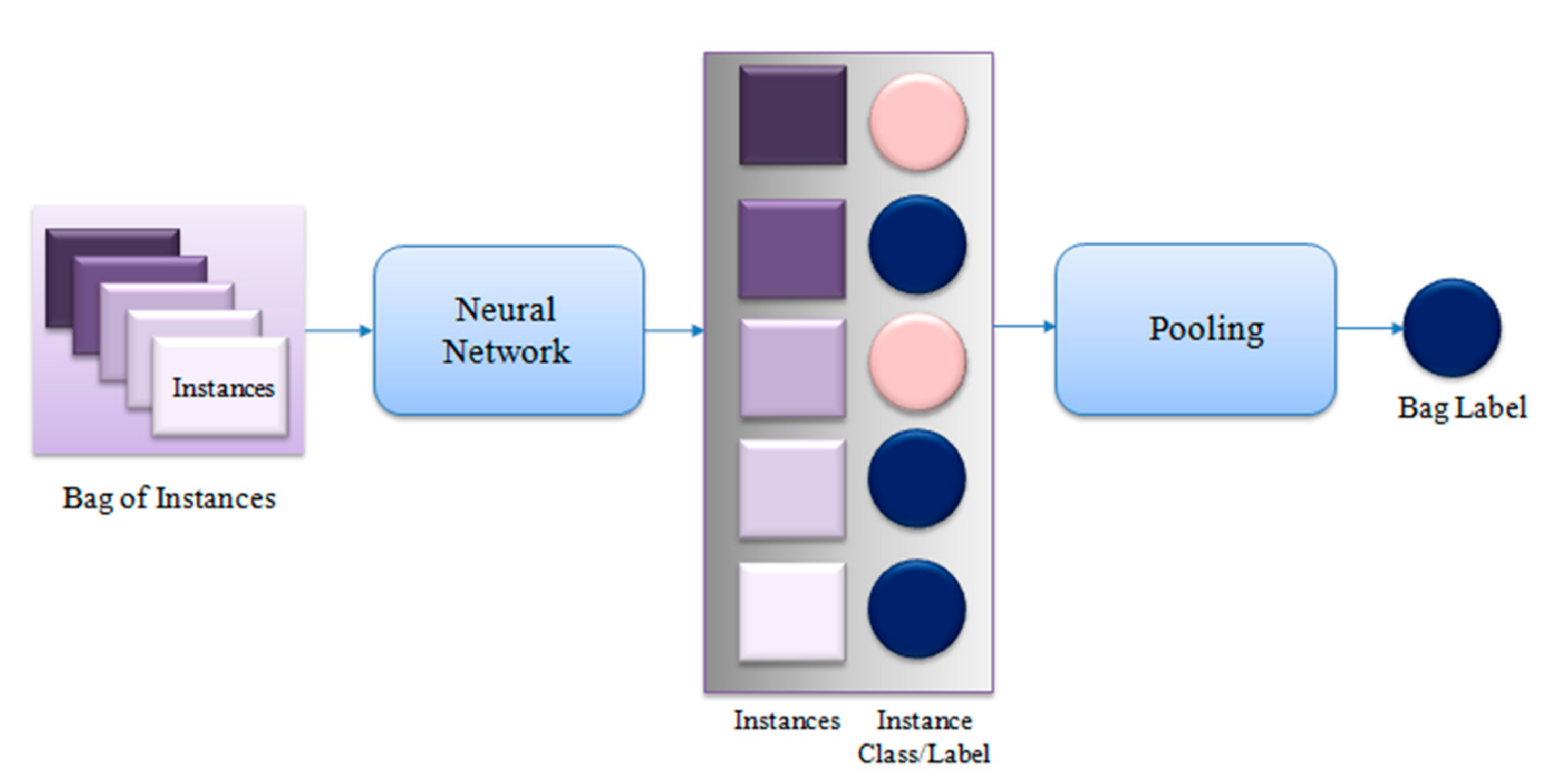
In case of general pooling methods—i.e., sum pooling, mean pooling, max pooling, or log-sum-exp pooling—a bag of instances is fed to the neural network, which generates the instance labels, and the pooling function extracts the bag label from these instance labels. This process is presented in Figure 2.
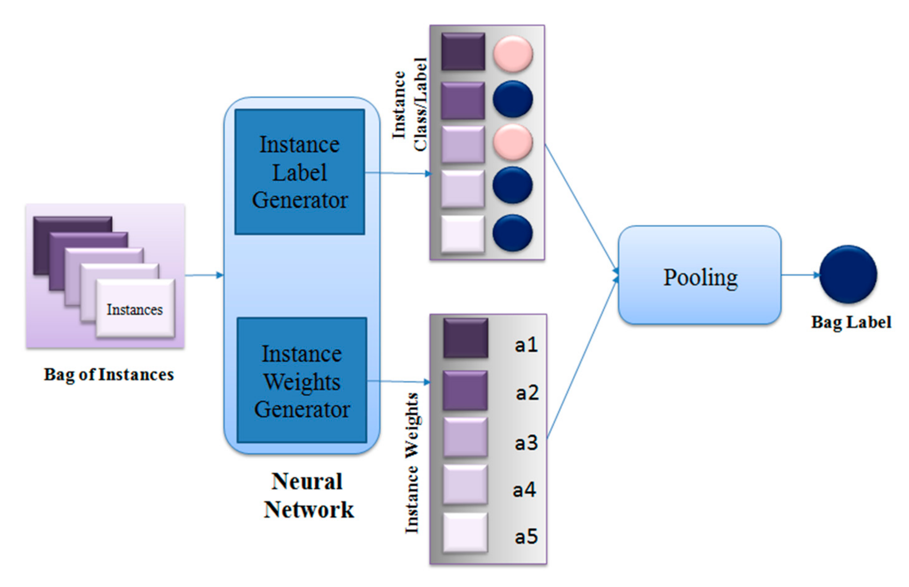
In attention-based and gated attention-based pooling, extra dense layers are used for generating instance weights; i.e., along with instance label generation, the neural network also generates instance weights. This instance weight generator is a fully connected layer that has three layers. Then, these instance labels and instance weights are used by attention-based and gated attention-based pooling functions to generate the bag labels. This process is presented in Figure 3.
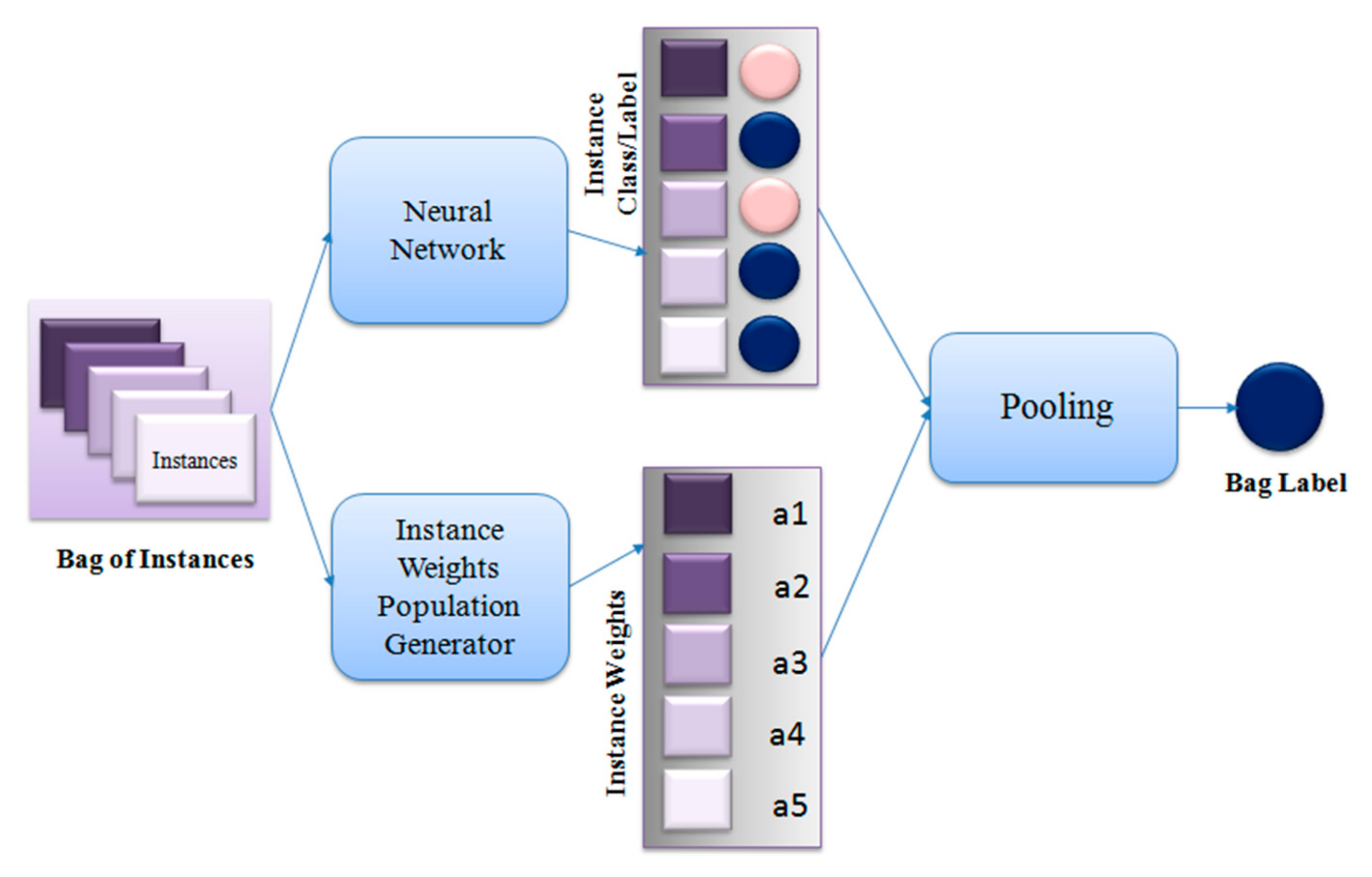
The evolutionary pooling function removes these extra layers for instance weight generation, as it randomly initializes a population of attention weights between [0, 1], and as the neural network trains, these weights are optimized simultaneously through DE or GA. For each set of weights representing the individuals of the population, the model is trained, and through a number of generations or passes, optimum values of the weights are obtained, thereby minimizing the loss. This process is presented in Figure 4.
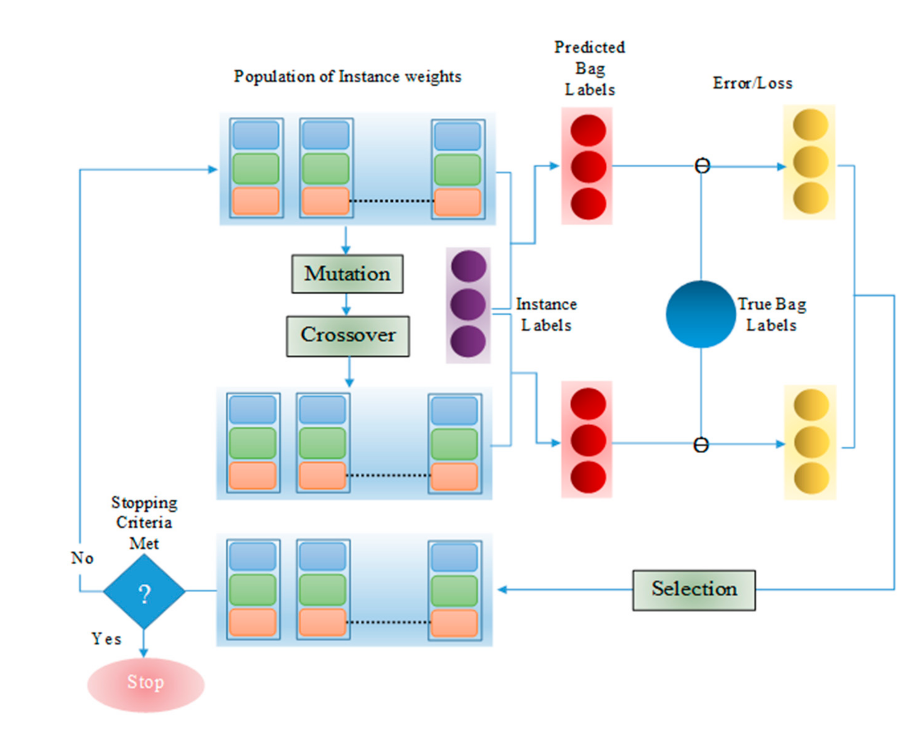
The instance weight optimization process through DE is presented in Figure 5. First, a population of instance weights is initialized with NP individuals. On the other hand, the neural network generates the instance labels. Now, using these instance labels and the population of instance weights, NP bag labels are predicted by the model (target bag labels). Then, through mutation and crossover operations, a trial population of instance weights is generated. Again, using instance labels and the trial population of instance weights, NP bag labels are predicted by the model (trial bag label). We already know the true bag labels, and thus the error in prediction or classification loss is calculated for both target bags as well as trial bags. Then, a tournament selection is performed for each individual for the target vector and trial vector. The vector with a smaller error is forwarded to the next generation. This process is repeated until the stopping criteria are met. An algorithm/pseudo-code for the MIL pooling function using DE is presented in Algorithm 1.
Algorithm 1. MIL Pooling Function using DE
● Set scaling factor F, crossover probability CR, Number of individuals in a population NP
● Set individual index, i = 1
● Set maximum iteration number max_iter
● Set iteration number, iter = 1
● Set number of bags P according to dataset
● Set bag number, p = 1
● Initialize population of instance weights a k for each bag with NP individuals
● While iter<= max_iter
   ○ While p <= P
      ■ While i<= NP
         ● Run feed-forward pass on neural network to generate instance labels
         ● Calculate bag label, z p s i g m o i d 1 K k = 1 K a k p h k p
         ● Calculate loss l z p for z p
         ● Generate 3 random numbers in [0,NP] – j1, j2, j3 where j1 ≠ j2 ≠ j3 ≠i
         ● Calculate mutant v p i = a p j 1 + F a p j 2 a p j 3
         ● dim = dimension of a p
         ● for d = 1:dim
            ○ Generate random number r in [0, 1] and random number d r a n d in [1,dim]
            ○ if r <= CR or d r a n d = d
               ■  u p i d =   v p i d
            ○ else
               ■  u p i d =   a p i d
         ● Calculate bag label for u k p , y p s i g m o i d 1 K k = 1 K u k p h k p
         ● Calculate loss l y p for y p
         ● If l y p < l z p
            ○  a p i =   u p i
The pooling function is independent of the neural network architecture. In this paper, the AMI-Net [10] is used. The architecture and experimental setup are the same as used in [8] to allow a comparison of the results with other pooling functions. The AMI-Net is described pictorially in Figure 6. First, through the embedding layer, each instance of the input (bag of instances) is mapped to a dense vector. Then, in the multi-head attention [41] layer, the intra-relationship of instances in different embedding subspaces is captured, where the subspaces represent the organs or body parts affected by a particular disease. These symptoms are often related to each other and are formulated mathematically by the multi-head attention layer. Then, to mine the instance correlations, layer normalization [42] and residual connection are used. In the next step, a set of fully-connected layers is employed to obtain the instance representations. These instance labels are obtained through instance-level pooling and act as the bag representations in bag-level pooling, where bag labels are obtained to classify the bags.
The DE parameters used include a scaling factor F of 0.5 and crossover probability CR of 0.8. Binary cross-entropy is used as the objective function to compute the loss between calculated and desired bag labels. Binary cross-entropy is used here as the dataset has two classes: schizophrenia relapse and non-relapse. The maximum number of iterations or epochs is set at 100. Experiments are done on five iterations of the dataset for fair comparison. To optimize the network, an Adam optimizer is used with a learning rate of0.00001, β1 = 0.9, β2 = 0.98, and ε = e−8.

5. Results and Discussion

5.1. Experimental Setup

The dataset used in [8,10,11] is used in this study; it is known as The Western Medicine (WM) dataset, which is a schizophrenia dataset of 3927 patients with 88 medical features. For a particular patient, there can be a maximum of 21 features and a minimum of 5 features. This dataset is quite imbalanced, with a positive rate of only 0.057. The objective of this work is to predict the possibility of relapse of a schizophrenic patient within a duration of three months.
The evaluation metrics used in this paper are the area under the curve (AUC), average precision (AP), accuracy, balanced accuracy, negative predictive value (NPV), specificity or true negative rate (TNR), Zero One loss, and Hamming loss.
Experiments were conducted with aSpyder 4.1.4 Integrated Development Environment (IDE) with Python 3.7.7 through an Anaconda distribution on an Intel Xeon Gold 6240 2.6 GHz dual processor system with 192 GB RAM, an Nvidia Quadro RTX 8000 GPU, and a 64-bit Windows 10 Education Operating System.

5.2. Results Analysis

Six bag-level pooling functions—max pooling, mean pooling, sum pooling, log-sum-exp pooling, gated attention-based pooling, and genetic pooling—were used to compare the proposed pooling function numerically as well as graphically. The pooling function designed through the basic DE variant was compared with other methods first to check whether it performed better than those methods. The numerical results obtained for different performance metrics are presented in Table 1. Highlighted values represent the best results obtained for each metric. The results in the table clearly indicate the robust performance of the proposed method, as it outperformed or performed on par with almost all the other methods used in this study. From a classification perspective, AUC is the most important evaluation metric for determining any classification model’s performance. In [8], it was shown that genetic pooling outperformed the other pooling functions in terms of AUC. Here, the DE pooling showed a significant increase in AUC (around 12% more than genetic pooling). DE considers real numbers, while for GA, it is necessary to work with a chromosomal representation of variables. Thus, in case of numerical optimization, DE tends to be more effective than GA. The strength of the Differential Evolution approach is that it often displays better results than a genetic algorithm and other evolutionary algorithms and can be easily applied to a wide variety of real valued problems despite noisy, multi-modal, and multi-dimensional spaces, which usually make the optimization of problems very difficult [43]. This paper deals with the numerical combinatorial optimization problem. The one-to-one spawning technique of DE explores the search space better thanGA; thus, DE provides better results than GA.
There is a great increase in terms of the Average Precision score, again establishing the superiority of DE pooling. The approach also exhibits higher accuracy and lower losses. DE pooling outperforms the other methods in every aspect.
The decaying value of loss is shown through the learning curves depicted in Figure 7. Here, it can be seen that DE pooling learning curve shows the same characteristics as genetic pooling. As the number of generations increases, genetic and DE pooling methods achieved the lowest loss value. Through this experiment, it was determined that, for metaheuristic approaches, increasing epochs results in a decrease in loss—i.e., better solutions—which is not the case for other methods. Generally, deep neural network models are trained with a large number of epochs, and thus metaheuristics-based pooling techniques are suitable in this case.
The training curves for GA and DE pooling are quite similar; i.e., they converge towards the same solution. Their accuracies are also not greatly different. Statistical analysis is needed when, even after comparing the algorithms, no concrete conclusion can be reached. Non-parametric statistical models are required in the case of evolutionary algorithms [44]. Here, the Wilcoxon rank-sum test or Mann–Whitney U test was used to determine which algorithm ranked higher in terms of various performance measurement metrics. This test is an alternative to the independent samples t-test when the assumptions required by the latter are not met by the data. It is used to compare differences between two independent groups (GA and DE in this case) when the dependent variable is either ordinal or continuous but not normally distributed. For this test, both algorithms were run for five iterations and the critical performance metrics—AUC, accuracy, balanced accuracy, NPV, and Zero One loss—were recorded. The Mann–Whitney test was applied through IBM SPSS software. The statistical results are presented in Table 2 and Table 3, where N represents the number of samples. Table 2 presents the rankings, while Table 3 shows the test statistics.
From Table 2, if we follow the mean rank, then it is clear that the DE pooling outranks the GA pooling in terms of AUC, accuracy, balanced accuracy, and NPV, but falls slightly behind in the case of loss. Furthermore, in Table 3, the Exact Sig. [2 × (1-tailed Sig.)] is the same as the p-value. For AUC and balanced accuracy, p 0.05 . Thus, we can reject the null hypothesis ( H 0 ) that “there are no significant differences between AUC values and balanced accuracy values of DE pooling and GA pooling”. However, for accuracy, NPV and Zero One Loss, p 0.05 . Thus, we cannot reject the null hypothesis ( H 0 ) that “there are no significant differences between accuracy values, NPV values and loss values of DE pooling and GA pooling”. Finally, from the non-parametric Mann–Whitney U Test results, it can be concluded that DE pooling significantly improves the AUC and balanced accuracy of the MIL model.
The comparisons of the basic DE approach and the variants SaDE, jDE, JADE and SHADE are presented in Table 4. The best result for each metric is highlighted in the table.
From Table 4, it can be seen that, for most of the evaluation metrics, the variants produce a better result. Although there is no clear winner among the DE variants, it can be concluded that parameter adaptation improves the MIL DE pooling.

6. Conclusions

A trainable MIL pooling function based on Differential Evolution (DE) is proposed in this paper and implemented with AMI-Net architecture. The validation of the method is conducted on The Western Medicine (WM) dataset, and the results are compared with well-known pooling functions such as max pooling, mean pooling, sum pooling, log-sum-exp pooling, gated attention pooling, and genetic pooling. Performance metrics used for comparison are the AUC, average precision Score, accuracy, balanced accuracy, NPV, Specificity/TNR, Zero One loss, and Hamming loss. It was observed that the proposed pooling function outperformed other approaches for all the metrics. Though there was no single best variant that outperformed others in every criterion, it is evident that parameter adaptation in DE improved the result. For future work, hybrid metaheuristic techniques can be explored in this case.

Author Contributions

Conceptualization, K.B.; methodology, K.B.; resources, M.P. and C.W.A.; data curation, K.B.; writing—original draft preparation, K.B. and A.T.; writing—review and editing, K.B., A.T. and M.P.; visualization, K.B. and A.T.; supervision, S.O. and C.W.A.; funding acquisition, S.O. and C.W.A. All authors have read and agreed to the published version of the manuscript.

Funding

This research was partly supported by the Korea government (MSIT) (No. 2019-0-01842, Artificial Intelligence Graduate School Program (GIST)) and GIST Research Institute (GRI) grant funded by the GIST in 2021.

Data Availability Statement

Data available in a publicly accessible repository that does not issue DOIs. Publicly available datasets were analyzed in this study. This data can be found here: https://github.com/Zeyuan-Wang/AMI-Net/blob/master/sample_data.xlsx (accessed on 31 March 2021).

Conflicts of Interest

The authors declare no conflict of interest. The funders had no role in the design of the study; in the collection, analyses, or interpretation of data; in the writing of the manuscript, or in the decision to publish the results.

References

  1. Cheplygina, V.; de Bruijne, M.; Pluim, J.P.W. Not-so-supervised: A survey of semi-supervised, multi-instance, and transfer learning in medical image analysis. Med. Image Anal. 2019, 54, 280–296. [Google Scholar] [CrossRef] [PubMed] [Green Version]
  2. Quellec, G.; Cazuguel, G.; Cochener, B.; Lamard, M. Multiple-Instance Learning for Medical Image and Video Analysis. IEEE Rev. Biomed. Eng. 2017, 10, 213–234. [Google Scholar] [CrossRef] [PubMed]
  3. Dietterich, T.G.; Lathrop, R.H.; Lozano-Pérez, T. Solving the multiple instance problem with axis-parallel rectangles. Artif. Intell. 1997, 89, 31–71. [Google Scholar] [CrossRef] [Green Version]
  4. Ramon, J.; De Raedt, L. Multi instance neural networks. In Proceedings of the ICML-2000 Workshop on Attribute-Value and Relational Learning, Stanford, CA, USA, 2 July 2000; pp. 53–60. [Google Scholar]
  5. Ilse, M.; Tomczak, J.M.; Welling, M. Attention-Based Deep Multiple Instance Learning. In Proceedings of the 35th International Conference on Machine Learning, Proceedings of Machine Learning Research (PMLR), Stockholm, Sweden, 10–15 July 2018; pp. 2127–2136. [Google Scholar]
  6. Yan, Y.; Wang, X.; Fang, J.; Liu, W.; Huang, J.; Zhu, J.; Takeuchi, I. Deep Multi-instance Learning with Dynamic Pooling. In Proceedings of the Asian Conference on Machine Learning, Beijing, China, 14–16 November 2018; pp. 1–16. [Google Scholar]
  7. Liu, D.; Zhou, Y.; Sun, X.; Zha, Z.; Zeng, W. Adaptive Pooling in Multi-instance Learning for Web Video Annotation. In Proceedings of the 2017 IEEE International Conference on Computer Vision Workshops (ICCVW), Venice, Italy, 22–29 October 2017; pp. 318–327. [Google Scholar]
  8. Bhattacharjee, K.; Pant, M.; Zhang, Y.D.; Satapathy, S.C. Multiple Instance Learning with Genetic Pooling for medical data analysis. Pattern Recognit. Lett. 2020, 133, 247–255. [Google Scholar] [CrossRef]
  9. Wang, X.; Yan, Y.; Tang, P.; Bai, X.; Liu, W. Revisiting multiple instance neural networks. Pattern Recognit. 2018, 74, 15–24. [Google Scholar] [CrossRef] [Green Version]
  10. Wang, Z.; Poon, J.; Sun, S.; Poon, S. Attention-based Multi-instance Neural Network for Medical Diagnosis from Incomplete and Low Quality Data. In Proceedings of the International Joint Conference on Neural Networks, Budapest, Hungary, 14–19 July 2019. [Google Scholar]
  11. Wang, Z.; Poon, J.; Poon, S. AMI-Net+: A Novel Multi-Instance Neural Network for Medical Diagnosis from Incomplete and Imbalanced Data. arXiv 2019, arXiv:1907.01734. [Google Scholar]
  12. Bhattacharjee, K.; Tiwari, A.; Pant, M.; Ahn, C.W. A Pooling Function based on Differential Evolution for Multiple Instance Learning. In Proceedings of the 9th International Conference on Smart Media and Applications (SMA 2020), Jeju, Korea, 17–19 September 2020. [Google Scholar]
  13. Storn, R.; Price, K. Differential Evolution—A Simple and Efficient Heuristic for Global Optimization over Continuous Spaces. J. Glob. Optim. 1997, 11, 341–359. [Google Scholar] [CrossRef]
  14. Qin, A.K.; Suganthan, P.N. Self-adaptive differential evolution algorithm for numerical optimization. In Proceedings of the 2005 IEEE Congress on Evolutionary Computation, IEEE CEC 2005, Edinburgh, UK, 2–5 September 2005; Volume 2, pp. 1785–1791. [Google Scholar]
  15. Brest, J.; Greiner, S.; Bošković, B.; Mernik, M.; Zumer, V. Self-adapting control parameters in differential evolution: A comparative study on numerical benchmark problems. IEEE Trans. Evol. Comput. 2006, 10, 646–657. [Google Scholar] [CrossRef]
  16. Zhang, J.; Sanderson, A.C. JADE: Adaptive differential evolution with optional external archive. IEEE Trans. Evol. Comput. 2009, 13, 945–958. [Google Scholar] [CrossRef]
  17. Tanabe, R.; Fukunaga, A. Success-history based parameter adaptation for Differential Evolution. In Proceedings of the 2013 IEEE Congress on Evolutionary Computation, CEC 2013, Cancun, Mexico, 20–23 June 2013; pp. 71–78. [Google Scholar]
  18. Carbonneau, M.-A.; Cheplygina, V.; Granger, E.; Gagnon, G. Multiple instance learning: A survey of problem characteristics and applications. Pattern Recognit. 2018, 77, 329–353. [Google Scholar] [CrossRef] [Green Version]
  19. Amores, J. Multiple instance classification: Review, taxonomy and comparative study. Artif. Intell. 2013, 201, 81–105. [Google Scholar] [CrossRef]
  20. Wang, S.; Zhu, Y.; Yu, L.; Chen, H.; Lin, H.; Wan, X.; Fan, X.; Heng, P.A. RMDL: Recalibrated multi-instance deep learning for whole slide gastric image classification. Med. Image Anal. 2019, 58, 101549. [Google Scholar] [CrossRef]
  21. Yousefi, M.; Krzyżak, A.; Suen, C.Y. Mass detection in digital breast tomosynthesis data using convolutional neural networks and multiple instance learning. Comput. Biol. Med. 2018, 96, 283–293. [Google Scholar] [CrossRef]
  22. Cao, P.; Ren, F.; Wan, C.; Yang, J.; Zaiane, O. Efficient multi-kernel multi-instance learning using weakly supervised and imbalanced data for diabetic retinopathy diagnosis. Comput. Med. Imaging Graph. 2018, 69, 112–124. [Google Scholar] [CrossRef]
  23. Liu, M.; Zhang, J.; Adeli, E.; Shen, D. Landmark-based deep multi-instance learning for brain disease diagnosis. Med. Image Anal. 2018, 43, 157–168. [Google Scholar] [CrossRef]
  24. Yao, J.; Zhu, X.; Jonnagaddala, J.; Hawkins, N.; Huang, J. Whole Slide Images based Cancer Survival Prediction using Attention Guided Deep Multiple Instance Learning Networks. Med. Image Anal. 2020, 65, 101789. [Google Scholar] [CrossRef]
  25. Bilal; Pant, M.; Zaheer, H.; Garcia-Hernandez, L.; Abraham, A. Differential Evolution: A review of more than two decades of research. Eng. Appl. Artif. Intell. 2020, 90, 103479. [Google Scholar] [CrossRef]
  26. Caraffini, F.; Kononova, A.V.; Corne, D. Infeasibility and structural bias in differential evolution. Inf. Sci. 2019, 496, 161–179. [Google Scholar] [CrossRef] [Green Version]
  27. Stanovov, V.; Akhmedova, S.; Semenkin, E. LSHADE Algorithm with Rank-Based Selective Pressure Strategy for Solving CEC 2017 Benchmark Problems. In Proceedings of the 2018 IEEE Congress on Evolutionary Computation, CEC 2018, Rio de Janeiro, Brazil, 8–13 July 2018. [Google Scholar]
  28. Awad, N.H.; Ali, M.Z.; Suganthan, P.N. Ensemble sinusoidal differential covariance matrix adaptation with Euclidean neighborhood for solving CEC2017 benchmark problems. In Proceedings of the 2017 IEEE Congress on Evolutionary Computation, CEC 2017, Donostia, Spain, 5–8 June 2017; Institute of Electrical and Electronics Engineers Inc.: New York, NY, USA, 2017; pp. 372–379. [Google Scholar]
  29. Awad, N.H.; Ali, M.Z.; Suganthan, P.N.; Reynolds, R.G. An ensemble sinusoidal parameter adaptation incorporated with L-SHADE for solving CEC2014 benchmark problems. In Proceedings of the 2016 IEEE Congress on Evolutionary Computation, CEC 2016, Vancouver, BC, Canada, 24–29 July 2016; Institute of Electrical and Electronics Engineers Inc.: New York, NY, USA, 2016; pp. 2958–2965. [Google Scholar]
  30. Yeh, J.F.; Chen, T.Y.; Chiang, T.C. Modified L-SHADE for Single Objective Real-Parameter Optimization. In Proceedings of the 2019 IEEE Congress on Evolutionary Computation, CEC 2019, Wellington, New Zealand, 10–13 June 2019; Institute of Electrical and Electronics Engineers Inc.: New York, NY, USA, 2019; pp. 381–386. [Google Scholar]
  31. Zhang, S.X.; Chan, W.S.; Tang, K.S.; Zheng, S.Y. Adaptive strategy in differential evolution via explicit exploitation and exploration controls. Appl. Soft Comput. 2021, 107, 107494. [Google Scholar] [CrossRef]
  32. Zeng, Z.; Zhang, M.; Chen, T.; Hong, Z. A new selection operator for differential evolution algorithm. Knowl. Based Syst. 2021, 226, 107150. [Google Scholar] [CrossRef]
  33. Salgotra, R.; Singh, U.; Saha, S.; Nagar, A. New Improved SALSHADE-cnEpSin Algorithm with Adaptive Parameters. In Proceedings of the 2019 IEEE Congress on Evolutionary Computation, CEC 2019, Wellington, New Zealand, 10–13 June 2019; Institute of Electrical and Electronics Engineers Inc.: New York, NY, USA, 2019; pp. 3150–3156. [Google Scholar]
  34. Han, G.; Chen, X. A Bi-level Differential Evolutionary Algorithm for Constrained Optimization. In Proceedings of the 2019 IEEE Congress on Evolutionary Computation, CEC 2019, Wellington, New Zealand, 10–13 June 2019; Institute of Electrical and Electronics Engineers Inc.: New York, NY, USA, 2019; pp. 1628–1633. [Google Scholar]
  35. Yang, Z.; Qiu, H.; Gao, L.; Jiang, C.; Chen, L.; Cai, X. A Novel Surrogate-assisted Differential Evolution for Expensive Optimization Problems with both Equality and Inequality Constraints. In Proceedings of the 2019 IEEE Congress on Evolutionary Computation, CEC 2019, Wellington, New Zealand, 10–13 June 2019; Institute of Electrical and Electronics Engineers Inc.: New York, NY, USA, 2019; pp. 1688–1695. [Google Scholar]
  36. Zheng, X.; Lei, Y.; Qin, A.K.; Zhou, D.; Shi, J.; Gong, M. Differential Evolutionary Multi-task Optimization. In Proceedings of the 2019 IEEE Congress on Evolutionary Computation, CEC 2019, Wellington, New Zealand, 10–13 June 2019; Institute of Electrical and Electronics Engineers Inc.: New York, NY, USA, 2019; pp. 1914–1921. [Google Scholar]
  37. Mousavirad, S.J.; Rahnamayan, S. A Novel Center-based Differential Evolution Algorithm. In Proceedings of the 2020 IEEE Congress on Evolutionary Computation, CEC 2020, Glasgow, UK, 19–24 July 2020; Institute of Electrical and Electronics Engineers Inc.: New York, NY, USA, 2020. [Google Scholar]
  38. Pant, M.; Vig, G. Clustering based Adaptive Differential Evolution for Numerical Optimization. In Proceedings of the 2020 IEEE Congress on Evolutionary Computation, CEC 2020, Glasgow, UK, 19–24 July 2020; Institute of Electrical and Electronics Engineers Inc.: New York, NY, USA, 2020. [Google Scholar]
  39. Kizilay, D.; Tasgetiren, M.F.; Oztop, H.; Kandiller, L.; Suganthan, P.N. A Differential Evolution Algorithm with Q-Learning for Solving Engineering Design Problems. In Proceedings of the 2020 IEEE Congress on Evolutionary Computation, CEC 2020, Glasgow, UK, 19–24 July 2020; Institute of Electrical and Electronics Engineers Inc.: New York, NY, USA, 2020. [Google Scholar]
  40. Jou, Y.C.; Wang, S.Y.; Yeh, J.F.; Chiang, T.C. Multi-population Modified L-SHADE for Single Objective Bound Constrained optimization. In Proceedings of the 2020 IEEE Congress on Evolutionary Computation, CEC 2020, Glasgow, UK, 19–24 July 2020; Institute of Electrical and Electronics Engineers Inc.: New York, NY, USA, 2020. [Google Scholar]
  41. Vaswani, A.; Brain, G.; Shazeer, N.; Parmar, N.; Uszkoreit, J.; Jones, L.; Gomez, A.N.; Kaiser, Ł.; Polosukhin, I. Attention is all you need. In Proceedings of the Advances in Neural Information Processing Systems, Long Beach, CA, USA, 4–9 December 2017; pp. 5998–6008. [Google Scholar]
  42. Ba, J.L.; Kiros, J.R.; Hinton, G.E. Layer Normalization. arXiv 2016, arXiv:1607.06450. [Google Scholar]
  43. Hegerty, B.; Hung, C.-C.; Kasprak, K. A Comparative Study on Differential Evolution and Genetic Algorithms for Some Combinatorial Problems. In Proceedings of the 8th Mexican International Conference on Artificial Intelligence, Guanajuato, Mexico, 9–13November 2009. [Google Scholar]
  44. Caraffini, F.; Iacca, G. The SOS platform: Designing, tuning and statistically benchmarking optimisation algorithms. Mathematics 2020, 8, 785. [Google Scholar] [CrossRef]
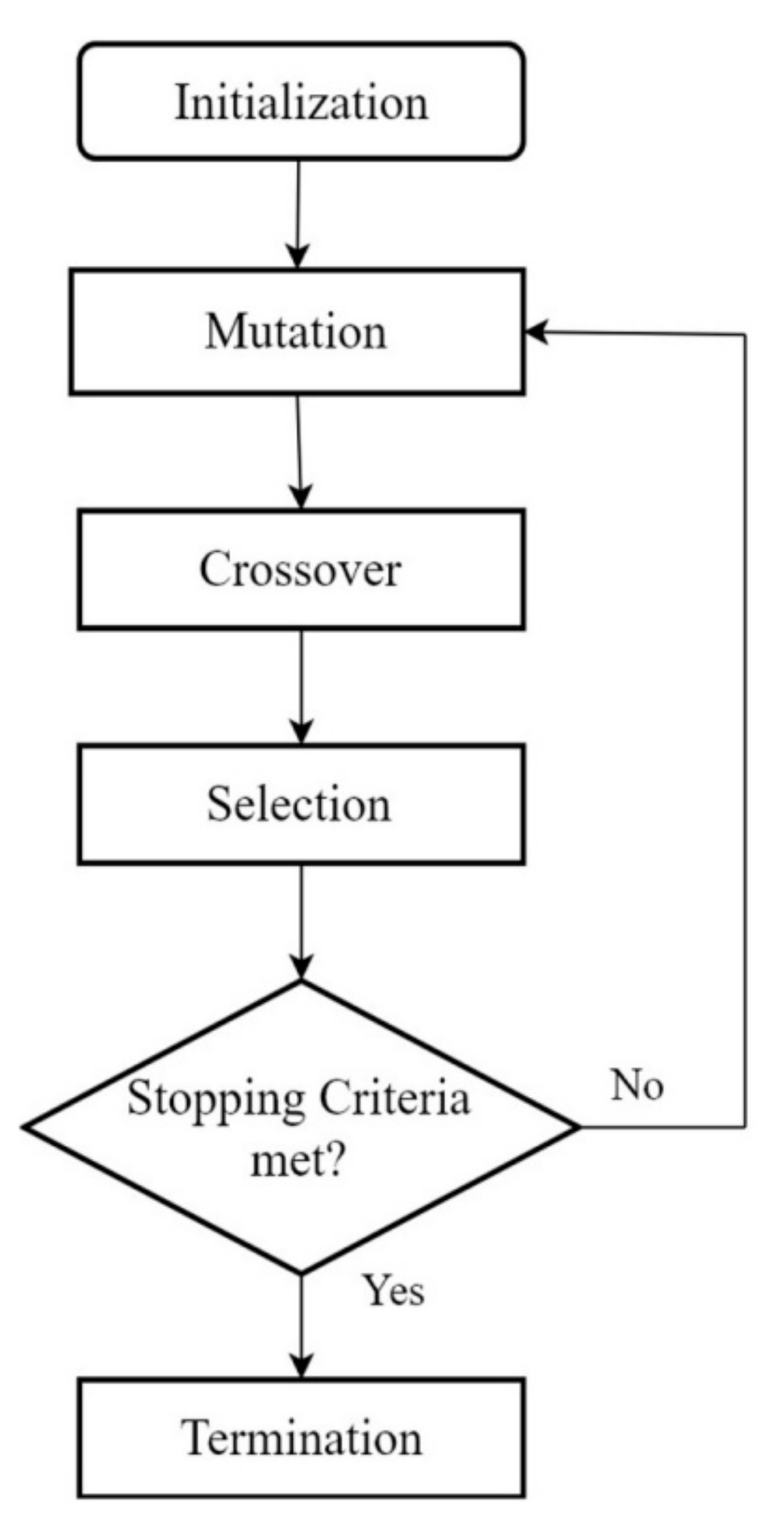
Figure 1. DE flowchart.
Electronics 10 01403 g001
Figure 2. General pooling functions.
Electronics 10 01403 g002
Figure 3. Attention-based pooling functions.
Electronics 10 01403 g003
Figure 4. Evolutionary pooling functions.
Electronics 10 01403 g004
Figure 5. Instance weight optimization through DE.
Electronics 10 01403 g005
Figure 6. AMI-Net with DE pooling.
Electronics 10 01403 g006
Figure 7. Learning curves.
Electronics 10 01403 g007
Table 1. Results (architecture = AMI-Net; dataset = WM).
MIL PoolingAUCAPAccuracyBalanced AccuracyNPVSpecificityZero One LossHamming Loss
Max pooling0.72833750.18791820.93775460.50265060.94275350.99432370.06224540.0622454
Mean pooling0.75219010.20065720.94184270.50912180.94354130.99798710.05815730.0581573
Sum pooling0.57555360.10037110.92014450.54010240.94725480.96970030.07985550.0798555
Log-sum-exp pooling0.73596050.18308310.94058480.51078790.94375240.99631930.05941520.0594152
Gated Attention pooling0.75447040.19582180.94247160.50239770.94274990.99966720.05752840.0575284
Genetic pooling0.88627810.37828980.94247160.50239770.94274990.99966720.05752840.0575284
DE pooling0.98380430.84290340.95378980.59835750.953276710.04621010.0462101
Table 2. Mann–Whitney U test rankings.
Ranks
AlgorithmNMean RankSum of Ranks
AUCGA53.0015.00
DE58.0040.00
Total10
AccuracyGA55.1025.50
DE55.9029.50
Total10
BalancedAccuracyGA53.5017.50
DE57.5037.50
Total10
NPVGA55.0025.00
DE56.0030.00
Total10
ZeroOneLossGA55.9029.50
DE55.1025.50
Total10
Table 3. Test statistics of Mann–Whitney U test.
Test Statistics a
AUCAccuracyBalancedAccuracyNPVZeroOneLoss
Mann–Whitney U0.00010.5002.50010.00010.500
Wilcoxon W15.00025.50017.50025.00025.500
Z−2.611−0.419−2.155−0.522−0.419
Asymp. Sig. (2-tailed)0.0090.6750.0310.6020.675
Exact Sig. [2x(1-tailed Sig.)]0.008 b0.690 b0.032 b0.690 b0.690 b
a Grouping variable: algorithm; b not corrected for ties.
Table 4. Comparison of DE variants.
VariantAUCAPAccuracyBalanced AccuracyNPVSpecificityZero One LossHamming Loss
DE0.68835910.12782990.94247160.50.942471610.05752840.0575284
SaDE0.67942180.14351110.94058580.50512590.94294680.99734870.05941420.0594142
jDE0.71013090.12852980.95125790.50747330.94260300.98660640.06916360.0691636
JADE0.69561480.12779940.94496860.50.942471610.05752840.0575284
SHADE0.72924170.13237760.95125790.50.942471610.05752840.0575284
Publisher’s Note: MDPI stays neutral with regard to jurisdictional claims in published maps and institutional affiliations.