
Security of Things Intrusion Detection System for Smart Healthcare

 ,
,  ,
,  and
and
Abstract
1. Introduction
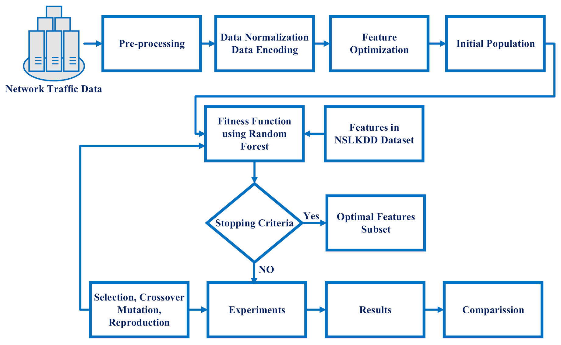
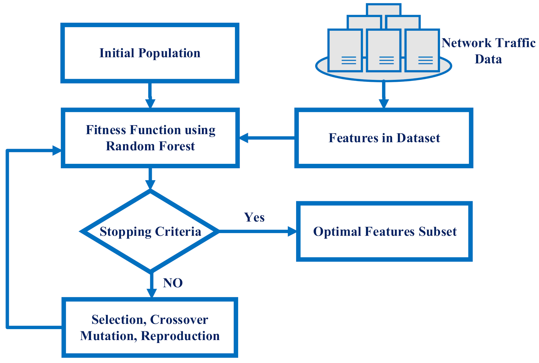
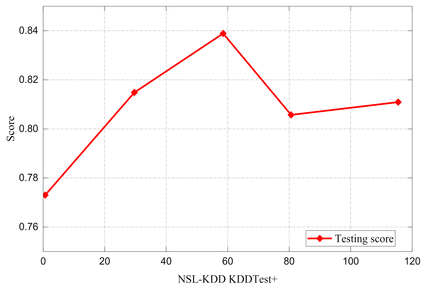
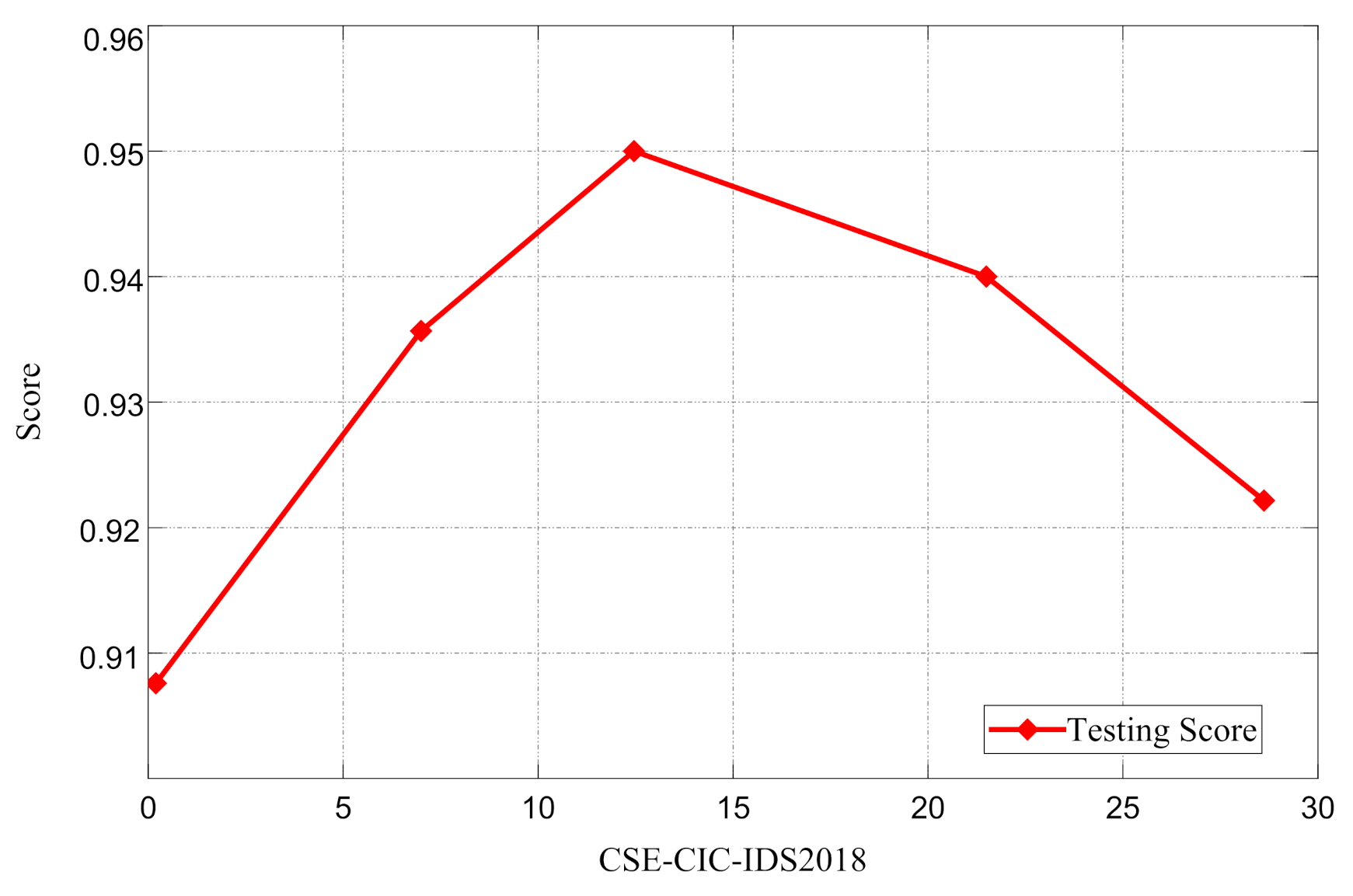
- In this research, after performing preprocessing on the NSL-KDD and CSE-CIC-IDS2018 datasets, all the features of both datasets were passed into the genetic algorithm fitness function. The Random Forest (RF) entropy function was utilized in the genetic algorithm fitness function to calculate the fitness values of the features. After the selection of optimal features, these features were again passed to an RF classifier to predict the network attacks. The newly proposed approach had the ability to use RF inside the genetic algorithm. Our main goal was to find the optimal feature subset using the genetic algorithm, and for this, we proposed a new fitness function, which was based on RF;
- This study also proposed the following weights for the genetic algorithm to obtain the optimal features from the NSL-KDD and CSE-CIC-IDS2018 datasets used in wireless communications systems. The parameters we updated were: SPX-crossover, crossover probability and random-init. These were implemented as an initialization operator for the genetic algorithm in this study. Moreover, bit-flip was employed as mutation operator with a mutation probability rate of and a population size of 200. The generational parameter was used as the replacement operator; the report frequency was set at 200; and the selection operator was the tournament selection, which was employed in this research;
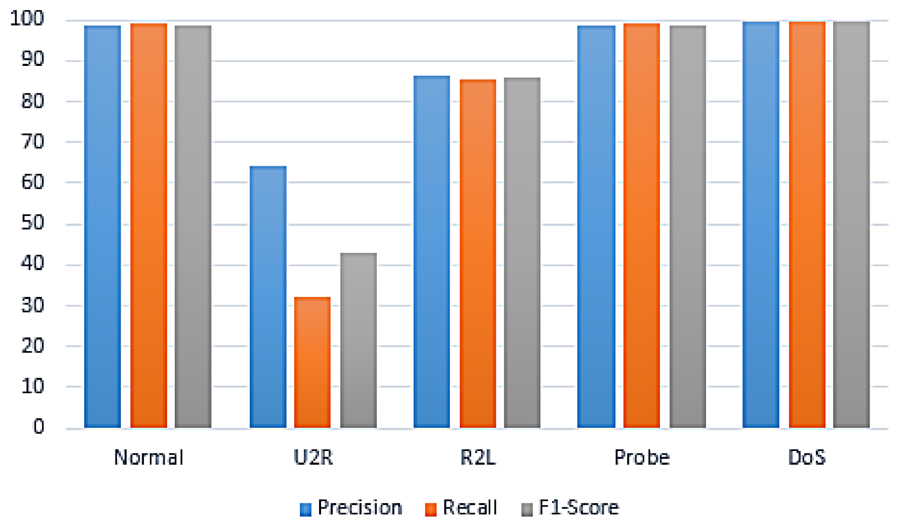
- The experimental results upheld the importance of feature optimization, which yielded better results considering the precision, recall, F1-measure, DR and FAR;
- The study of J. Ren et al achieved a 92.8% accuracy and a 33% false alarm rate with the DO-IDS method [13]. Their findings also indicated an 86.5% accuracy and a 12.4% false alarm rate using the traditional genetic algorithm and RF classifier. However, our proposed model, which was a combination of the genetic algorithm and RF (GA-RF), outperformed these results at 98.81% DR and 0.8% FAR, respectively;
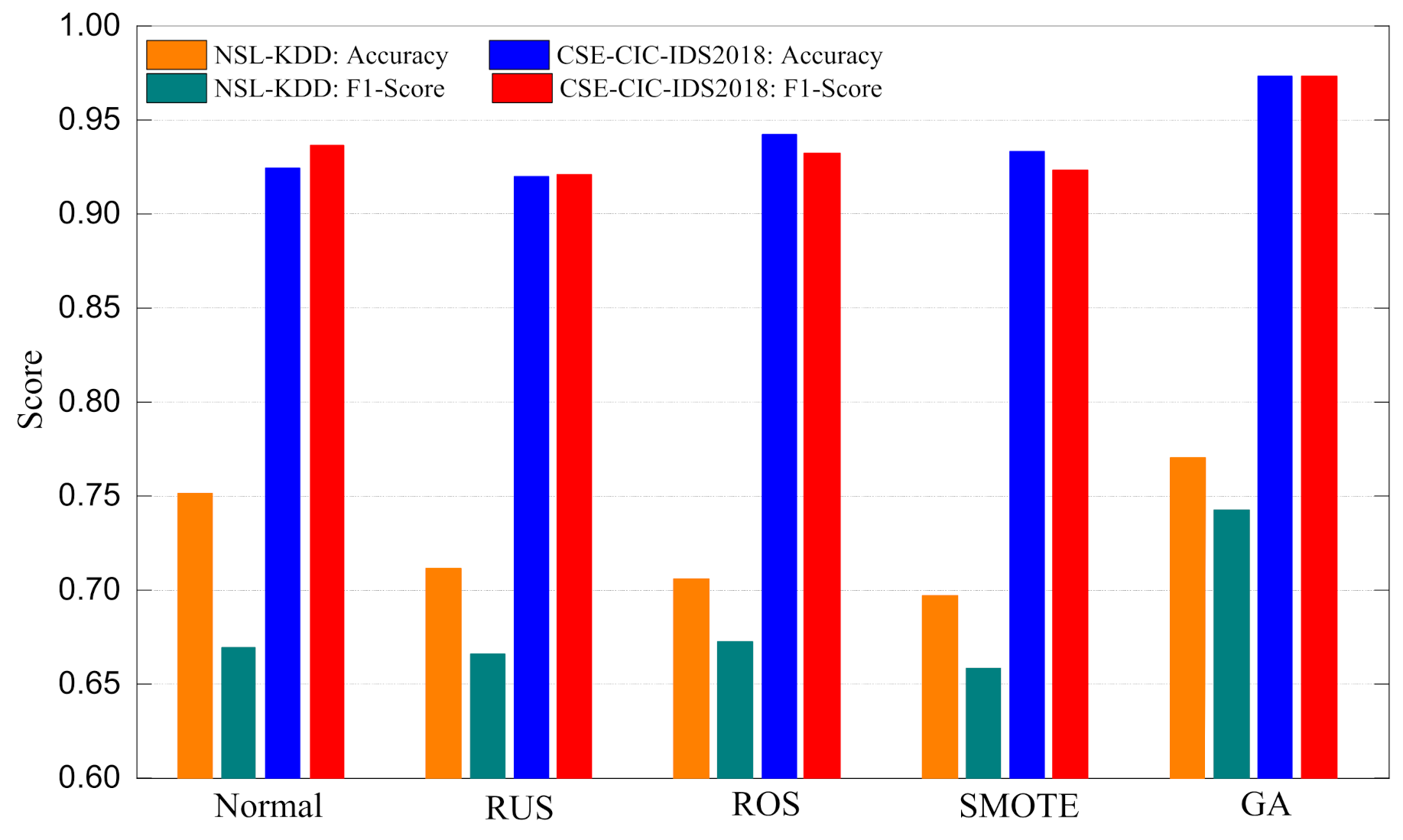
- The results showed that the proposed GA was greatly optimized, in which the average precision was optimized by 5.65%, and the average F1-score was optimized by 8.2%.
Research Organization
2. Literature Review
3. Proposed Methodology
3.1. NSL-KDD Dataset
- 10 continuous (features: 1, 5, 6, 10, 11, 13, 16, 17, 18, 19);
- 4 categorical (features: 2, 3, 4, 42);
- 23 discrete (features: 8, 9, 15, 23 to 41, 43);
- 6 binary (features: 7, 12, 14, 20, 21, 22).
3.2. Data Normalization (Min-Max Method)
3.3. Optimal Feature Selection Using Evolutionary Search
| Algorithm 1: Pseudocode of the genetic algorithm |
 |
3.4. Machine Learning Algorithms
- Random forest:Multiple decision trees are combined to build an RF classifier. The purpose of the RF classier is that it assembles numerous decision trees to give more meaningful and precise results. For regression, it calculates the mean of every decision tree and assigns the mean value to the predicted variable. For classification cases, the RF employs a majority vote approach. For example, if 3 trees predicated yes and 2 trees predicated no, then it will assign yes to the predicated variable. Entropy and information gain are used for deciding the root or parent node of the tree [41] and give the following known equations.where represents the probabilities of the class labels:
- Logistic regression:Another popular and well-known machine learning algorithm used for classification is logistic regression. Typically, logistic regression produces more dichotomous results. The working methodology of logistic regression is that it finds a correlation among final output values and also provides the characteristics. In logistic regression, the log odds function is used for prediction.
- Naive Bayes:NB is a supervised machine learning technique. NB is a probability machine learning model used for classification. In this research, we used a traditional NB classifier for the predication of various attacks.
3.5. Evaluation Metrics
4. Experiments and Results
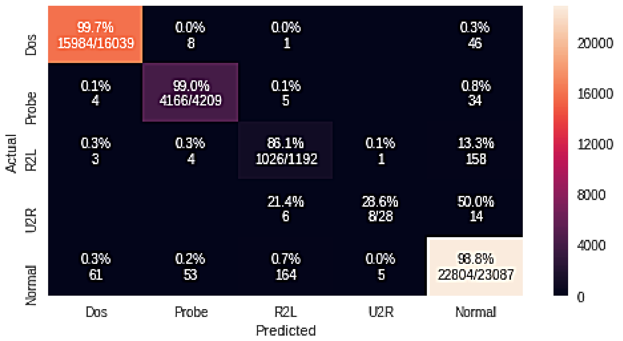
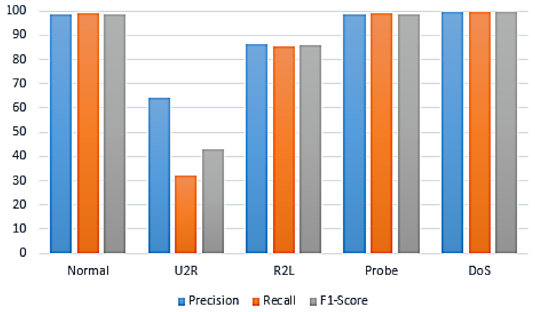
4.1. Random Forest Attack Experiment Results
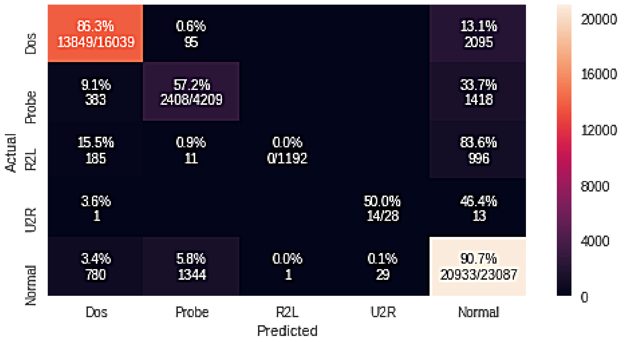
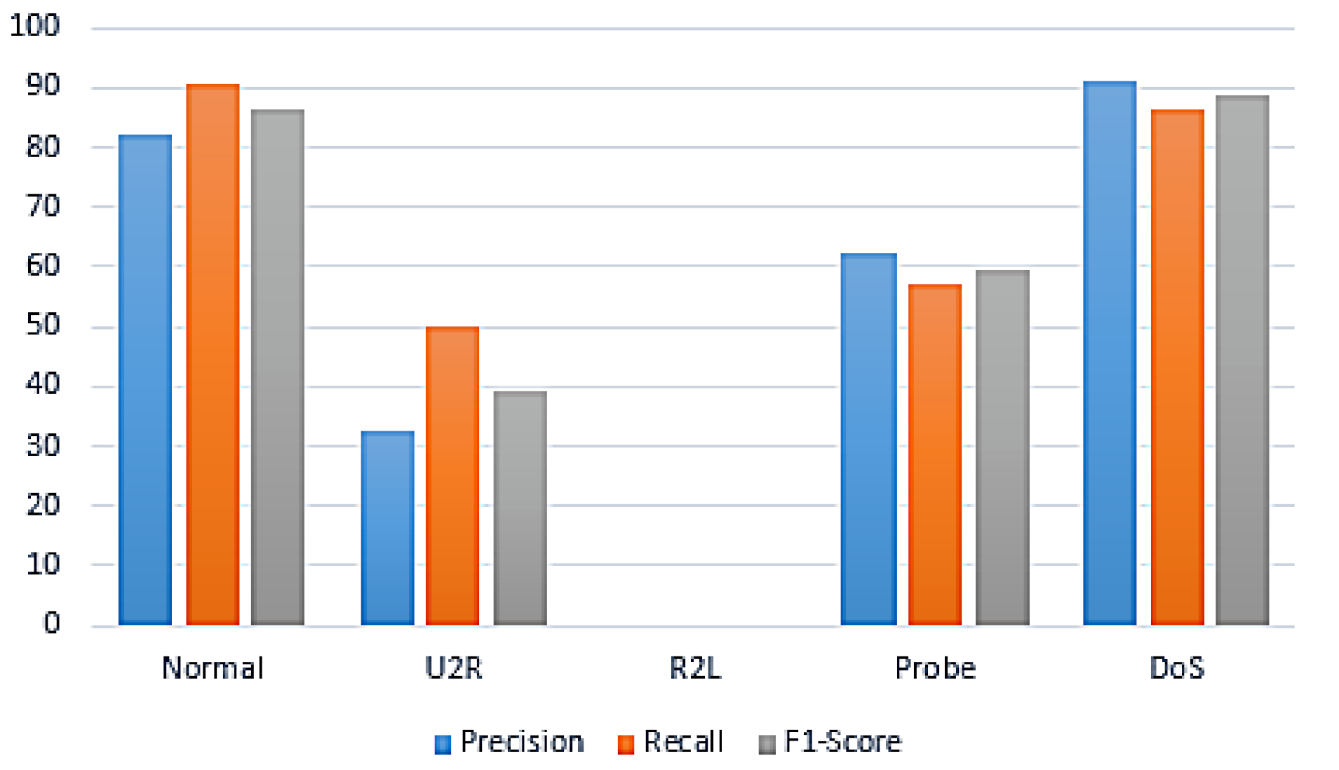
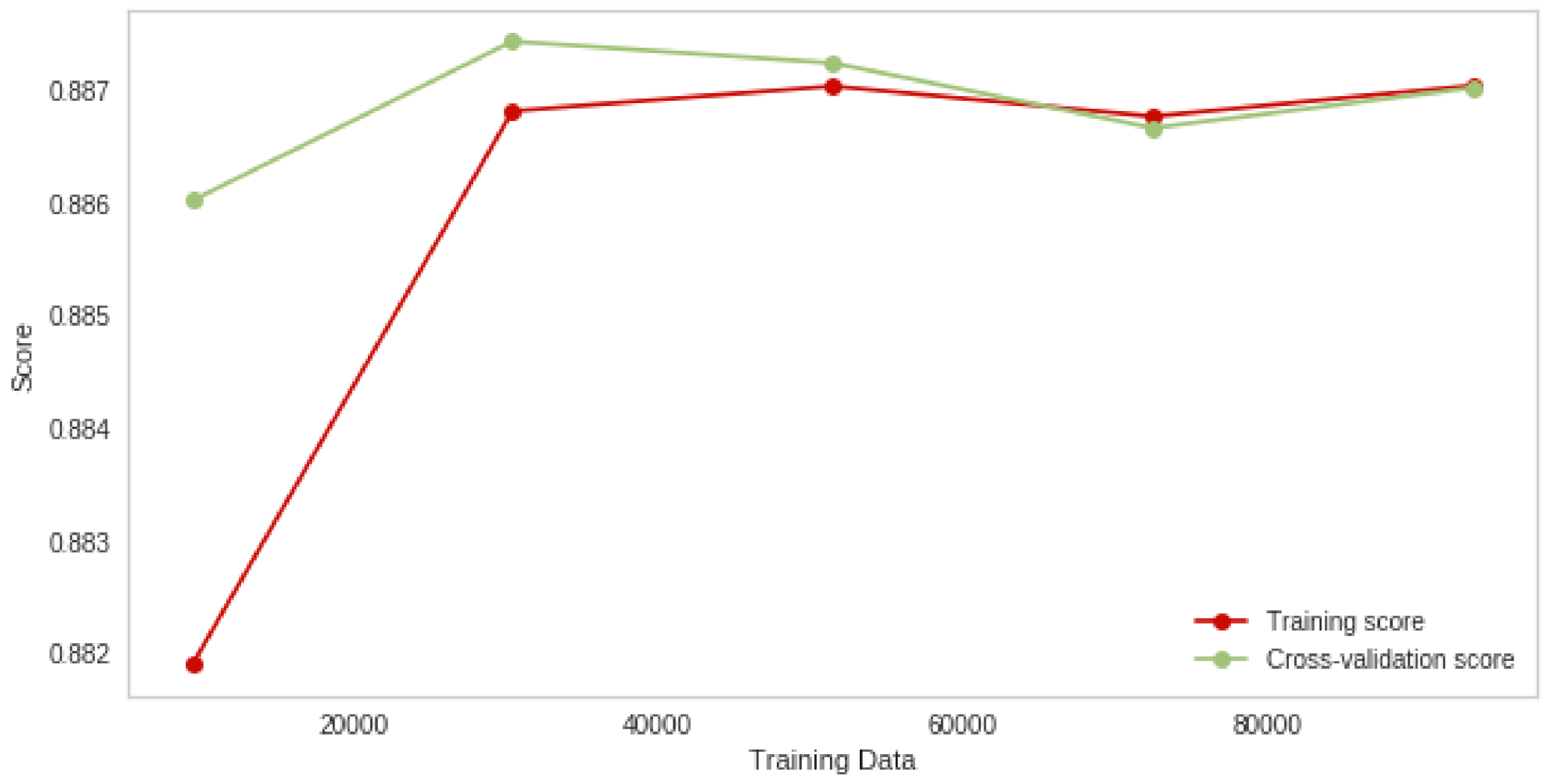
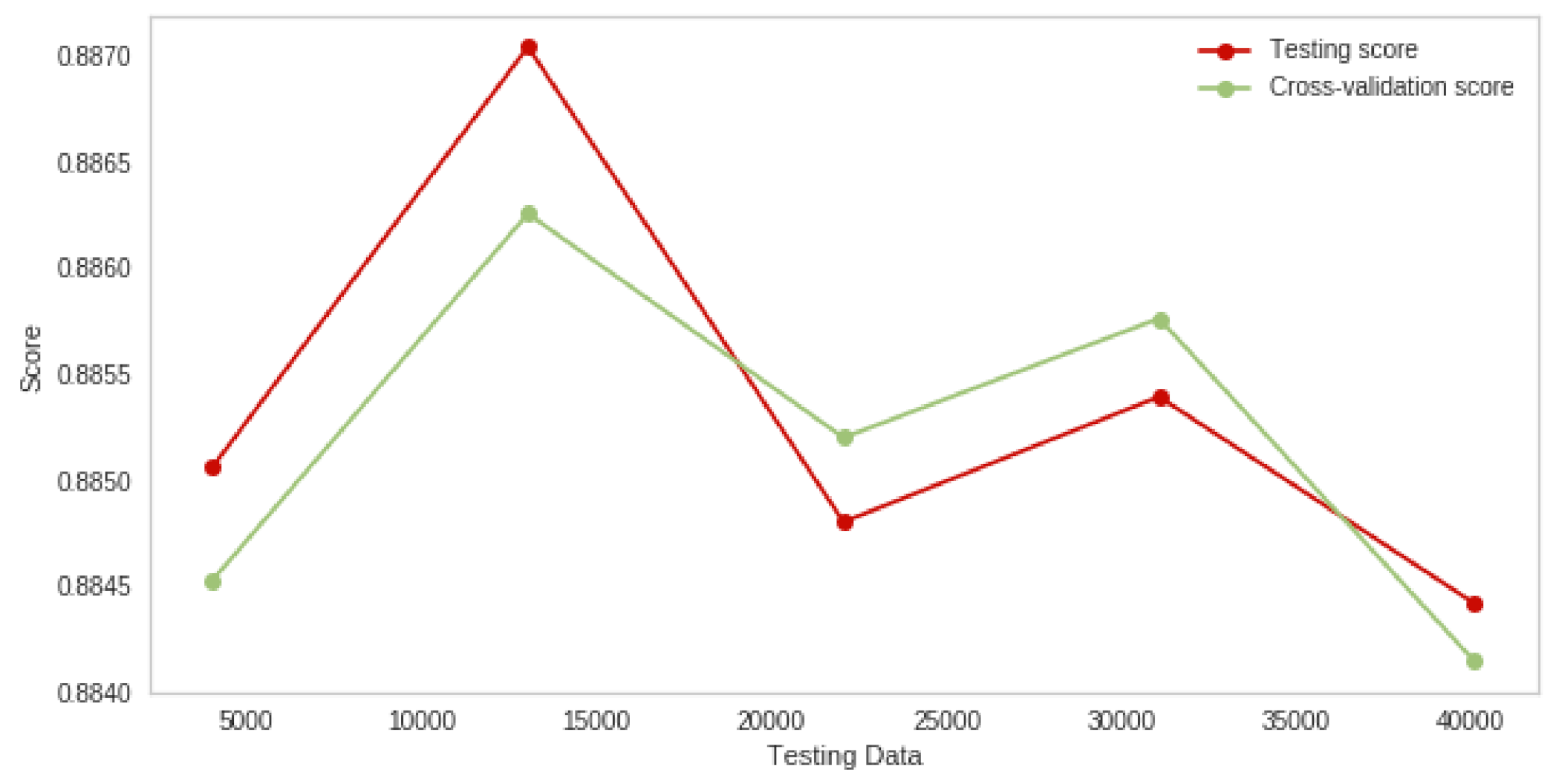
4.2. Naive Bayes Classifier Experimental Results
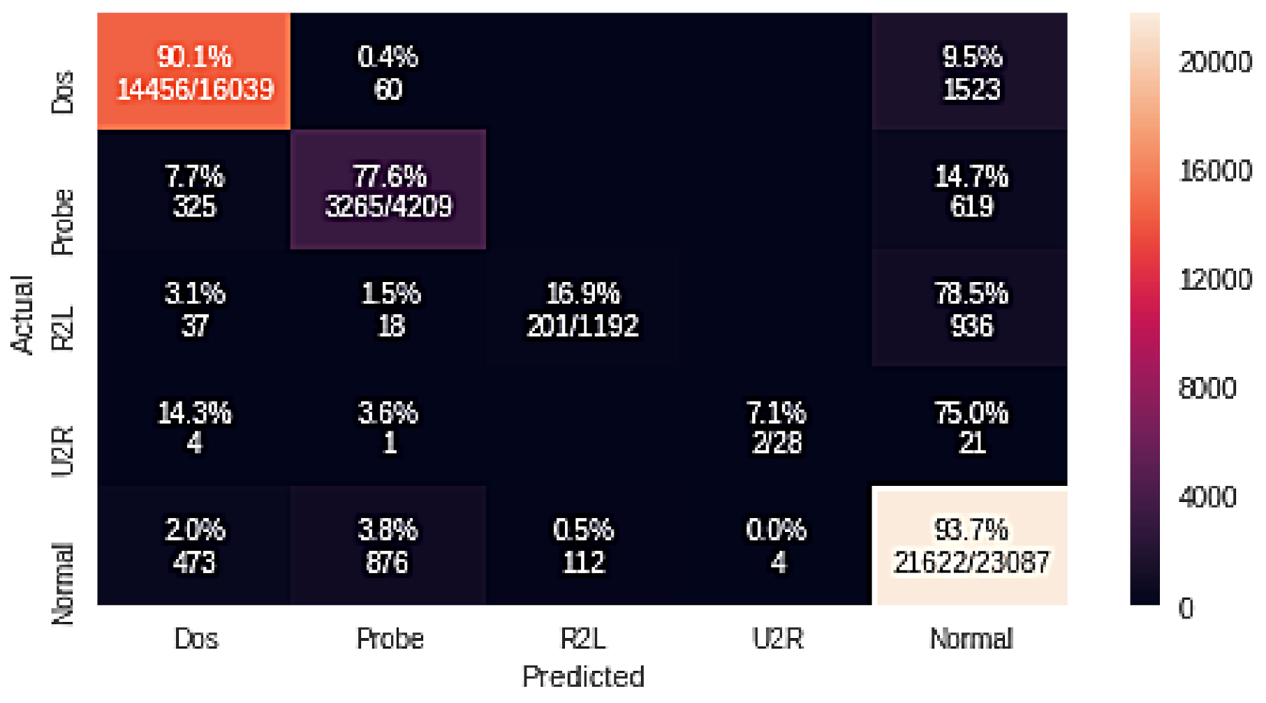
4.3. Logistic Regression Classifier Experiment Results for Multiple Attacks
4.4. Binary Class Experimental Results
4.4.1. Random Forest Classifier Experiment Results for the Binary Class
4.4.2. Naive Bayes Experiment Results for the Binary Class
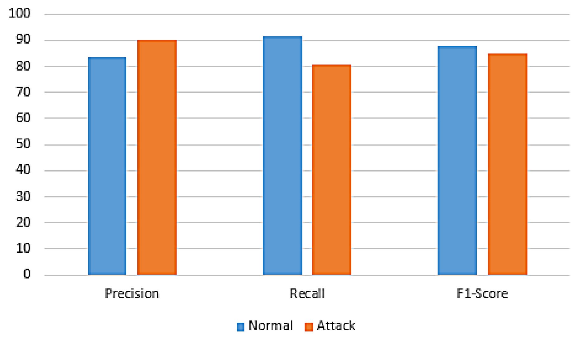
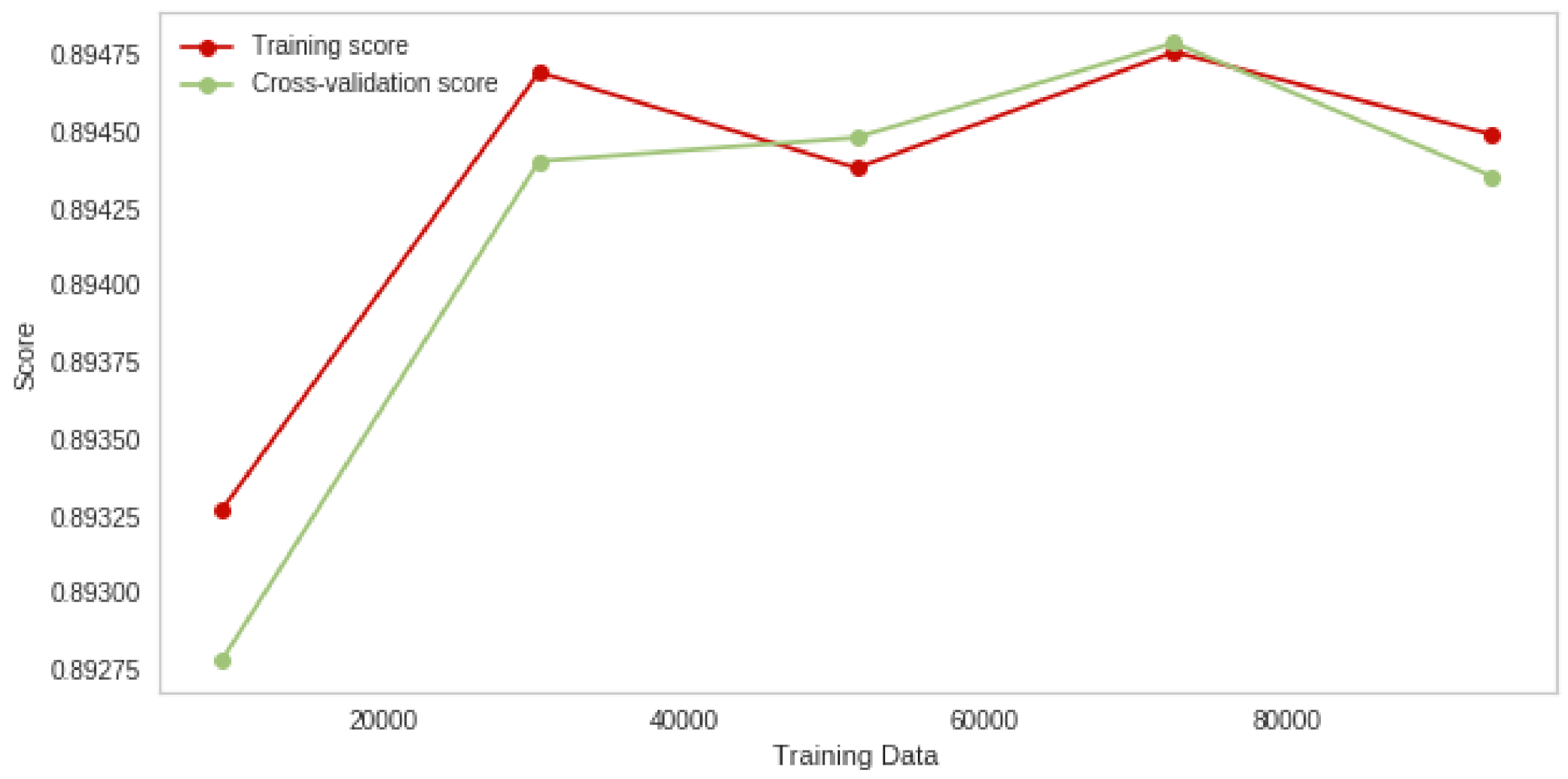
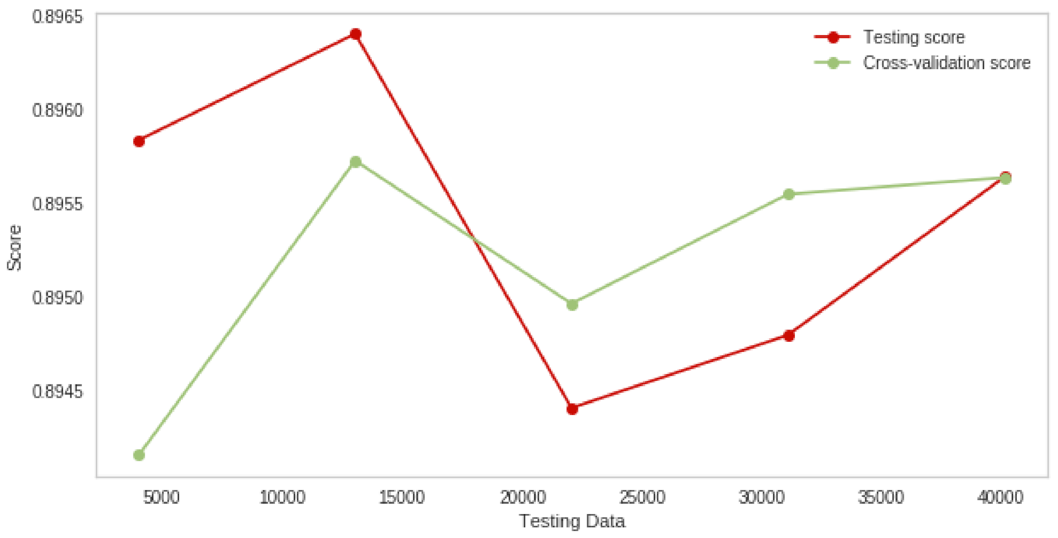
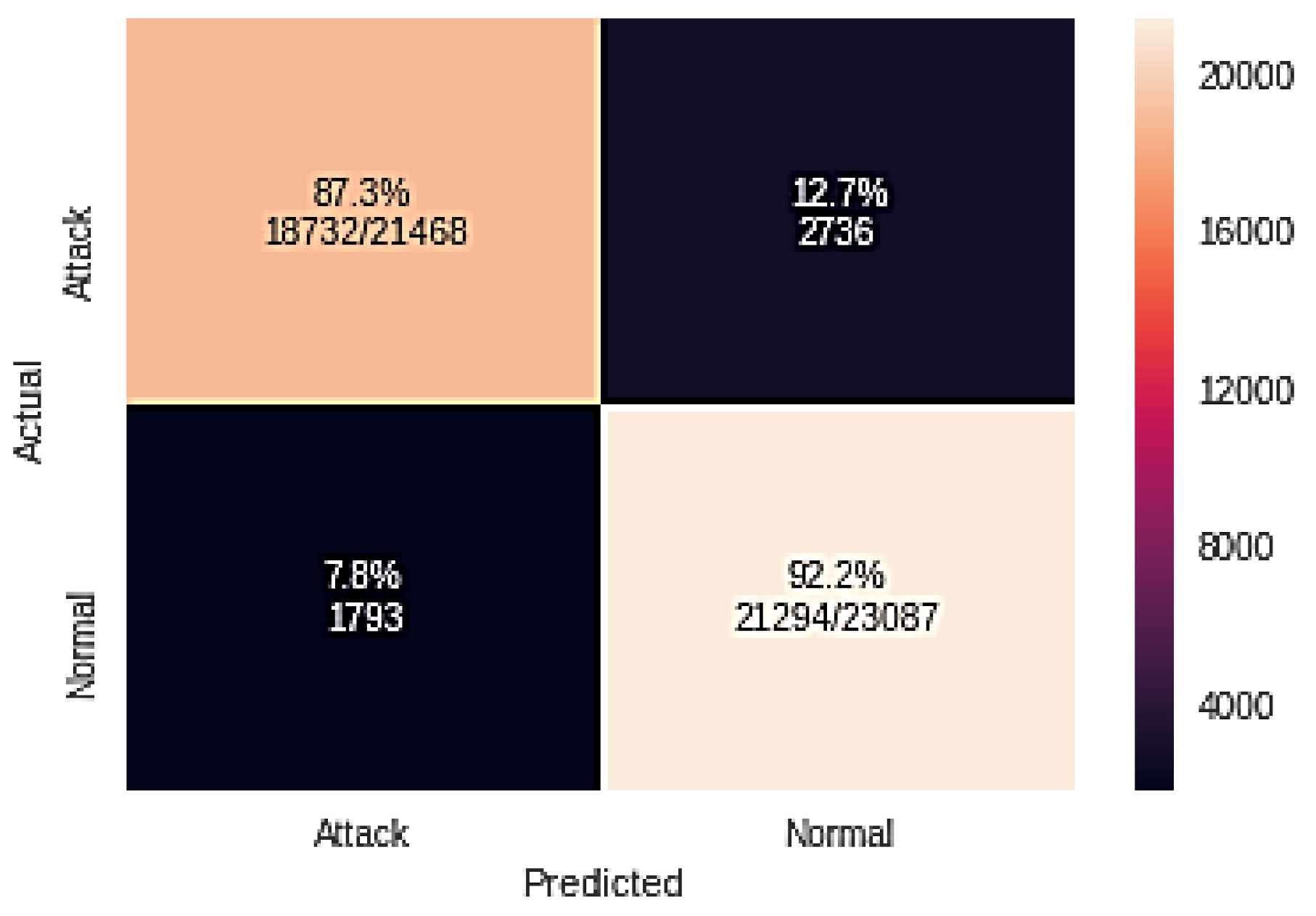
4.4.3. Logistic Regression Experiment Results for the Binary Class
4.5. Discussion
5. Conclusions
Author Contributions
Funding
Conflicts of Interest
References
- Zhang, S.; Xie, X.; Xu, Y. A Brute-Force Black-Box Method to Attack Machine Learning-Based Systems in Cybersecurity. IEEE Access 2020, 8, 128250–128263. [Google Scholar] [CrossRef]
- Hady, A.A.; Ghubaish, A.; Salman, T.; Unal, D.; Jain, R. Intrusion Detection System for Healthcare Systems Using Medical and Network Data: A Comparison Study. IEEE Access 2020, 8, 106576–106584. [Google Scholar] [CrossRef]
- Ullah, A.; Azeem, M.; Ashraf, H.; Alaboudi, A.A.; Humayun, M.; Jhanjhi, N. Secure Healthcare Data Aggregation and Transmission in IoT—A Survey. IEEE Access 2021, 9, 16849–16865. [Google Scholar] [CrossRef]
- Anajemba, J.H.; Tang, Y.; Iwendi, C.; Ohwoekevwo, A.; Srivastava, G.; Jo, O. Realizing Efficient Security and Privacy in IoT Networks. Sensors 2020, 20, 2609. [Google Scholar] [CrossRef] [PubMed]
- Anajemba, J.H.; Yue, T.; Iwendi, C.; Chatterjee, P.; Ngabo, D.; Alnumay, W.S. A Secure Multi-user Privacy Technique for Wireless IoT Networks using Stochastic Privacy Optimization. IEEE Internet Things J. 2021, 1. [Google Scholar] [CrossRef]
- Hussain, F.; Abbas, S.G.; Shah, G.A.; Pires, I.M.; Fayyaz, U.U.; Shahzad, F.; Garcia, N.M.; Zdravevski, E. A Framework for Malicious Traffic Detection in IoT Healthcare Environment. Sensors 2021, 21, 3025. [Google Scholar] [CrossRef] [PubMed]
- Elrawy, M.F.; Awad, A.I.; Hamed, H.F.A. Intrusion detection systems for IoT-based smart environments: A survey. J. Cloud Comput. 2018, 7, 21–29. [Google Scholar] [CrossRef]
- Bhattacharya, S.; Ramakrishnan, S.S.; Maddikunta, P.K.R.; Kaluri, R.; Singh, S.; Gadekallu, T.R.; Alazab, M.; Tariq, U. A Novel PCA-Firefly based XGBoost classification model for Intrusion Detection in Networks using GPU. Electronics 2020, 9, 219. [Google Scholar] [CrossRef]
- Liu, G.; Yi, Z.; Yang, S. A hierarchical intrusion detection model based on the PCA neural networks. Neurocomputing 2007, 70, 1561–1568. [Google Scholar] [CrossRef]
- Heba, F.E.; Darwish, A.; Hassanien, A.E.; Abraham, A. Principle components analysis and support vector machine based intrusion detection system. In Proceedings of the 2010 10th International Conference on Intelligent Systems Design and Applications, Cairo, Egypt, 29 November–1 December 2010; pp. 363–367. [Google Scholar]
- Chae, H.S.; Jo, B.O.; Choi, S.H.; Park, T.K. Feature selection for intrusion detection using NSL-KDD. Recent Adv. Comput. Sci. 2013, 32, 184–187. [Google Scholar]
- Sarmah, A. Intrusion Detection Systems: Definition, Need and Challenges; SANS Institute: Bethesda, MD, USA, 2001. [Google Scholar]
- Ren, J.; Guo, J.; Qian, W.; Yuan, H.; Hao, X.; Jingjing, H. Building an effective intrusion detection system by using hybrid data optimization based on machine learning algorithms. Secur. Commun. Netw. 2019, 2019. [Google Scholar] [CrossRef]
- Thamilarasu, G.; Odesile, A.; Hoang, A. An Intrusion Detection System for Internet of Medical Things. IEEE Access 2020, 8, 181560–181576. [Google Scholar] [CrossRef]
- Vaiyapuri, T.; Binbusayyis, A.; Varadarajan, V. Security, Privacy and Trust in IoMT Enabled Smart Healthcare System: A Systematic Review of Current and Future Trends. Int. J. Adv. Comput. Sci. Appl. 2021, 12. [Google Scholar] [CrossRef]
- Cook, D.J.; Duncan, G.; Sprint, G.; Fritz, R.L. Using Smart City Technology to Make Healthcare Smarter. Proc. IEEE 2018, 106, 708–722. [Google Scholar] [CrossRef]
- Belavagi, M.C.; Muniyal, B. Performance evaluation of supervised machine learning algorithms for intrusion detection. Procedia Comput. Sci. 2016, 89, 117–123. [Google Scholar] [CrossRef]
- Almseidin, M.; Alzubi, M.; Kovacs, S.; Alkasassbeh, M. Evaluation of machine learning algorithms for intrusion detection system. In Proceedings of the 2017 IEEE 15th International Symposium on Intelligent Systems and Informatics (SISY), Subotica, Serbia, 14–16 September 2017; pp. 277–282. [Google Scholar]
- Chen, L.S.; Syu, J.S. Feature extraction based approaches for improving the performance of intrusion detection systems. In Proceedings of the International MultiConference of Engineers and Computer Scientists, Hong Kong, China, 18–20 March 2015; Volume 1, pp. 18–20. [Google Scholar]
- De la Hoz, E.; De La Hoz, E.; Ortiz, A.; Ortega, J.; Prieto, B. PCA filtering and probabilistic SOM for network intrusion detection. Neurocomputing 2015, 164, 71–81. [Google Scholar] [CrossRef]
- Wagh, S.K.; Pachghare, V.K.; Kolhe, S.R. Survey on intrusion detection system using machine learning techniques. Int. J. Comput. Appl. 2013, 78, 30–37. [Google Scholar]
- Qiu, C.; Shan, J.; Shandong, B. Research on intrusion detection algorithm based on BP neural network. Int. J. Secur. Its Appl. 2015, 9, 247–258. [Google Scholar] [CrossRef]
- Taher, K.A.; Jisan, B.M.Y.; Rahman, M.M. Network intrusion detection using supervised machine learning technique with feature selection. In Proceedings of the 2019 International Conference on Robotics, Electrical and Signal Processing Techniques (ICREST), Dhaka, Bangladesh, 10–12 January 2019; pp. 643–646. [Google Scholar]
- Mukherjee, S.; Sharma, N. Intrusion detection using naive Bayes classifier with feature reduction. Procedia Technol. 2012, 4, 119–128. [Google Scholar] [CrossRef]
- Li, Y.; Xia, J.; Zhang, S.; Yan, J.; Ai, X.; Dai, K. An efficient intrusion detection system based on support vector machines and gradually feature removal method. Expert Syst. Appl. 2012, 39, 424–430. [Google Scholar] [CrossRef]
- Eesa, A.S.; Orman, Z.; Brifcani, A.M.A. A novel feature-selection approach based on the cuttlefish optimization algorithm for intrusion detection systems. Expert Syst. Appl. 2015, 42, 2670–2679. [Google Scholar] [CrossRef]
- Kumar, K.; Batth, J.S. Network intrusion detection with feature selection techniques using machine-learning algorithms. Int. J. Comput. Appl. 2016, 150, 1–13. [Google Scholar] [CrossRef]
- Syarif, A.R.; Gata, W. Intrusion detection system using hybrid binary PSO and K-nearest neighbourhood algorithm. In Proceedings of the 2017 11th International Conference on Information & Communication Technology and System (ICTS), Surabaya, Indonesia, 31 October 2017; pp. 181–186. [Google Scholar]
- Aghdam, M.H.; Kabiri, P. Feature Selection for Intrusion Detection System Using Ant Colony Optimization. IJ Netw. Secur. 2016, 18, 420–432. [Google Scholar]
- Mahmood, D.I.; Hameed, S.M. A Feature Selection Model based on Genetic Algorithm for Intrusion Detection. Iraqi J. Sci. 2016, 168–175. [Google Scholar]
- Rai, K.; Devi, M.S.; Guleria, A. Decision tree based algorithm for intrusion detection. Int. J. Adv. Netw. Appl. 2016, 7, 2828. [Google Scholar]
- Thaseen, S.; Kumar, C.A. Intrusion Detection Model using PCA and Ensemble of Classiers. Adv. Syst. Sci. Appl. 2016, 16, 15–38. [Google Scholar]
- Ambusaidi, M.A.; He, X.; Nanda, P.; Tan, Z. Building an intrusion detection system using a filter-based feature selection algorithm. IEEE Trans. Comput. 2016, 65, 2986–2998. [Google Scholar] [CrossRef]
- Bamakan, S.M.H.; Wang, H.; Yingjie, T.; Shi, Y. An effective intrusion detection framework based on MCLP/SVM optimized by time-varying chaos particle swarm optimization. Neurocomputing 2016, 199, 90–102. [Google Scholar] [CrossRef]
- Thaseen, I.S.; Kumar, C.A. Intrusion detection model using fusion of chi-square feature selection and multi class SVM. J. King Saud Univ. Comput. Inf. Sci. 2017, 29, 462–472. [Google Scholar]
- Pajouh, H.H.; Dastghaibyfard, G.; Hashemi, S. Two-tier network anomaly detection model: A machine learning approach. J. Intell. Inf. Syst. 2017, 48, 61–74. [Google Scholar] [CrossRef]
- Shone, N.; Ngoc, T.N.; Phai, V.D.; Shi, Q. A deep learning approach to network intrusion detection. IEEE Trans. Emerg. Top. Comput. Intell. 2018, 2, 41–50. [Google Scholar] [CrossRef]
- Naseer, S.; Saleem, Y.; Khalid, S.; Bashir, M.K.; Han, J.; Iqbal, M.M.; Han, K. Enhanced network anomaly detection based on deep neural networks. IEEE Access 2018, 6, 48231–48246. [Google Scholar] [CrossRef]
- Woo, J.H.; Song, J.Y.; Choi, Y.J. Performance Enhancement of Deep Neural Network Using Feature Selection and Preprocessing for Intrusion Detection. In Proceedings of the 2019 International Conference on Artificial Intelligence in Information and Communication (ICAIIC), Okinawa, Japan, 11–13 February 2019; pp. 415–417. [Google Scholar]
- Tao, P.; Sun, Z.; Sun, Z. An improved intrusion detection algorithm based on GA and SVM. IEEE Access 2018, 6, 13624–13631. [Google Scholar] [CrossRef]
- Negandhi, P.; Trivedi, Y.; Mangrulkar, R. Intrusion Detection System Using Random Forest on the NSL-KDD Dataset. In Emerging Research in Computing, Information, Communication and Applications; Springer: Berlin/Heidelberg, Germany, 2019; pp. 519–531. [Google Scholar]
- Pervez, M.S.; Farid, D.M. Feature selection and intrusion classification in NSL-KDD cup 99 dataset employing SVMs. In Proceedings of the 8th International Conference on Software, Knowledge, Information Management and Applications (SKIMA 2014), Dhaka, Bangladesh, 18–20 December 2014; pp. 1–6. [Google Scholar]
- Kanakarajan, N.K.; Muniasamy, K. Improving the accuracy of intrusion detection using GAR-Forest with feature selection. In Proceedings of the 4th International Conference on Frontiers in Intelligent Computing: Theory and Applications (FICTA), Durgapur, India, 16–18 November 2015; pp. 539–547. [Google Scholar]
- Raman, M.G.; Somu, N.; Kirthivasan, K.; Liscano, R.; Sriram, V.S. An efficient intrusion detection system based on hypergraph-Genetic algorithm for parameter optimization and feature selection in support vector machine. Knowl. Based Syst. 2017, 134, 1–12. [Google Scholar] [CrossRef]
- Kuang, F.; Xu, W.; Zhang, S. A novel hybrid KPCA and SVM with GA model for intrusion detection. Appl. Soft Comput. 2014, 18, 178–184. [Google Scholar] [CrossRef]
- Singh, R.; Kumar, H.; Singla, R. An intrusion detection system using network traffic profiling and online sequential extreme learning machine. Expert Syst. Appl. 2015, 42, 8609–8624. [Google Scholar] [CrossRef]
- De La Hoz, E.; Ortiz, A.; Ortega, J.; De la Hoz, E. Network anomaly classification by support vector classifiers ensemble and non-linear projection techniques. In Proceedings of the International Conference on Hybrid Artificial Intelligence Systems, Salamanca, Spain, 11–13 September 2013; pp. 103–111. [Google Scholar]
- Tavallaee, M.; Bagheri, E.; Lu, W.; Ghorbani, A.A. A detailed analysis of the KDD CUP 99 data set. In Proceedings of the 2009 IEEE Symposium on Computational Intelligence for Security and Defense Applications, Ottawa, ON, Canada, 8–10 July 2009; pp. 1–6. [Google Scholar]
- Tsang, C.H.; Kwong, S.; Wang, H. Genetic-fuzzy rule mining approach and evaluation of feature selection techniques for anomaly intrusion detection. Pattern Recognit. 2007, 40, 2373–2391. [Google Scholar] [CrossRef]
- Kayacik, H.G.; Zincir-Heywood, A.N.; Heywood, M.I. A hierarchical SOM-based intrusion detection system. Eng. Appl. Artif. Intell. 2007, 20, 439–451. [Google Scholar] [CrossRef]
- Raman, M.G.; Somu, N.; Kirthivasan, K.; Sriram, V.S. A hypergraph and arithmetic residue-based probabilistic neural network for classification in intrusion detection systems. Neural Netw. 2017, 92, 89–97. [Google Scholar] [CrossRef]


| Author | Year | Feature Selection Approach | Feature Type | Dataset | Classifier |
|---|---|---|---|---|---|
| Mahmood et al. [30] | 2016 | Information Gain Genetic Algorithm | Single | NSLKDD | Naive Bayes |
| K. Rai et al. [31] | 2016 | Information Gain | Single | NSLKDD | Decision Tree |
| Thaseen et al. [32] | 2016 | PCA | Single | NSLKDD UNSW-NB | SVM LDC QDC WMA |
| M. Ambusaidi et al. [33] | 2016 | FMIFS | Single | KDD99 NSLKDD Kyoto2006 | LSSVM |
| Bamakan et al. [34] | 2016 | TVCPSO | Single | NSLKDD | SVM |
| Thaseen et al. [35] | 2017 | Chi | Single | NSLKDD | SVM |
| Pajouh et al. [36] | 2017 | - | - | NSLKDD | Deep Learning |
| Shone et al. [37] | 2018 | - | - | NSLKDD | RNN |
| Naseer et al. [38] | 2018 | - | - | NSLKDD | LSTM |
| Woo et al. [39] | 2019 | Correlation Method | Ensemble | NSLKDD | NN |
| Classifier Name | DoS | Probe | R2L | U2R | Normal |
|---|---|---|---|---|---|
| Random Forest + GA | 99.7 | 99.0 | 86.1 | 28.6 | 98.8 |
| Naive Bayes + GA | 86.3 | 57.2 | 0.0 | 50.0 | 90.7 |
| Logistic Regression + GA | 90.1 | 77.6 | 16.9 | 7.1 | 93.7 |
| Classifier Name | Training Accuracy | Testing Accuracy |
|---|---|---|
| Random Forest + GA | 99.4 | 98.7 |
| Naive Bayes + GA | 83.4 | 83.5 |
| Logistic Regression + GA | 88.8 | 88.7 |
| Classifier | Attacks | Precision | Recall | F1-Measure |
|---|---|---|---|---|
| DoS | 99.60 | 99.60 | 99.60 | |
| Probe | 98.70 | 98.90 | 98.80 | |
| RF + GA | R2L | 86.50 | 85.30 | 85.90 |
| U2R | 64.30 | 32.10 | 42.90 | |
| Normal | 98.80 | 98.90 | 98.80 | |
| DoS | 91.10 | 86.30 | 88.70 | |
| Probe | 62.40 | 57.20 | 59.70 | |
| NB + GA | R2L | 0.0 | 0.0 | 0.0 |
| U2R | 32.60 | 50.00 | 39.40 | |
| Normal | 88.20 | 90.70 | 86.20 | |
| DoS | 94.50 | 90.10 | 92.30 | |
| Probe | 77.40 | 77.60 | 77.50 | |
| LR + GA | R2L | 64.20 | 16.90 | 26.70 |
| U2R | 33.33 | 7.10 | 11.80 | |
| Normal | 87.50 | 93.70 | 90.50 |
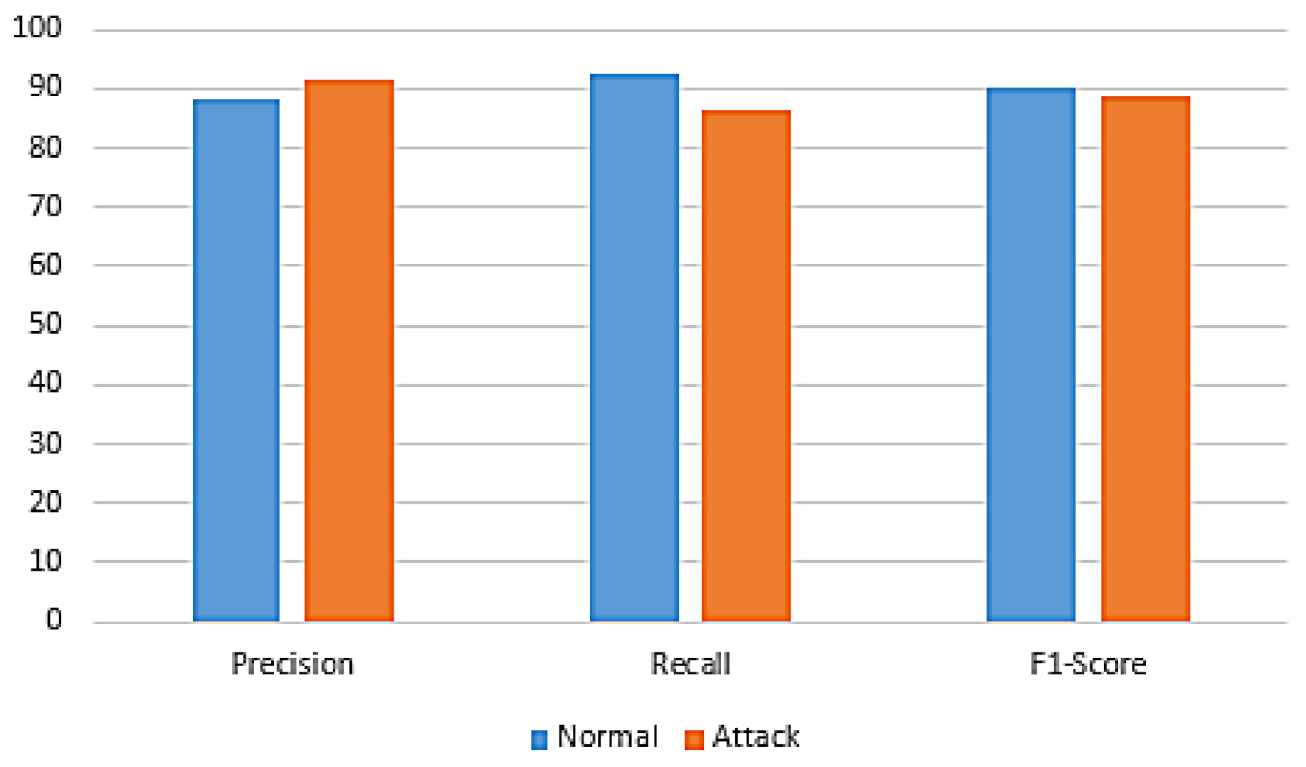
| Classifier Name | Class Label | Precision | Recall | F1-Measure |
|---|---|---|---|---|
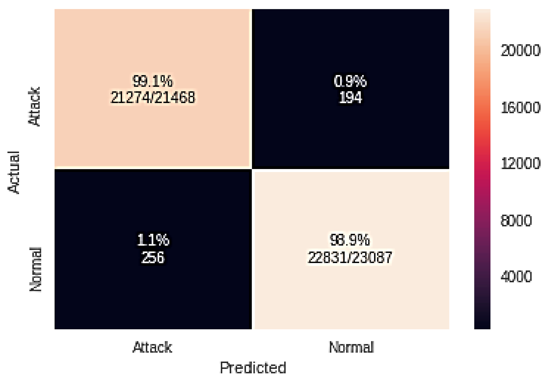
| GA + RF | Normal | 99.10 | 99.10 | 99.10 |
| Attack | 99.00 | 99.00 | 99.00 | |
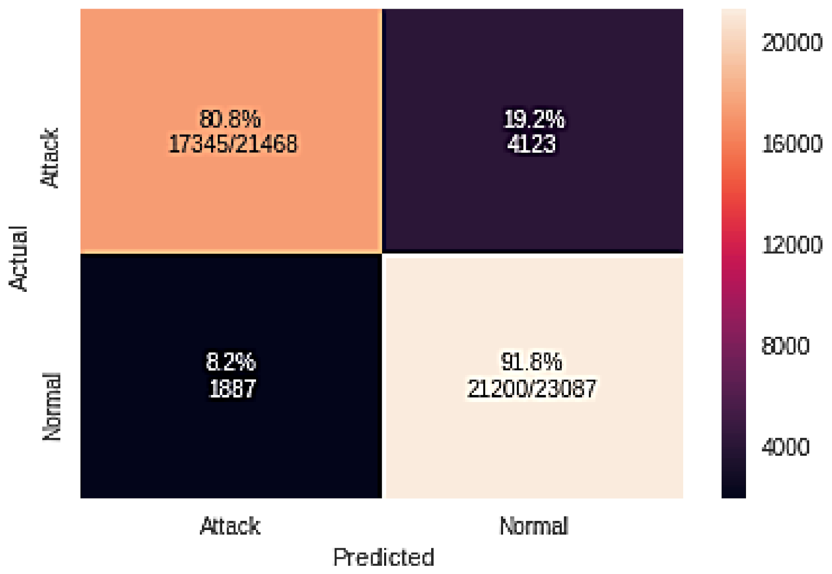
| GA + NB | Normal | 83.70 | 91.80 | 87.60 |
| Attack | 90.20 | 80.80 | 85.20 | |
| GA + LG | Normal | 88.10 | 92.40 | 90.20 |
| Attack | 91.40 | 86.60 | 88.90 |
| Classifier Name | TP | FN | FP | TN |
|---|---|---|---|---|
| GA + RF | 21274 | 256 | 194 | 22,831 |
| GA + NB | 17345 | 1887 | 4123 | 21,200 |
| GA + LG | 18732 | 1973 | 2736 | 21,294 |
| Model | Training Accuracy % | Testing Accuracy % | FAR | DR % |
|---|---|---|---|---|
| GA + RF | 99.73 | 99.10 | 0.008 | 98.81 |
| GA + NB | 88.00 | 86.50 | 00.16 | 90.18 |
| GA + LG | 89.65 | 91.31 | 00.11 | 90.47 |
| Authors | Detection Rate % | FAR % |
|---|---|---|
| Mahmood et al. [30] | 98.00 | 1.96 |
| Bamakan et al. [34] | 97.03 | 0.87 |
| Pajouh et al. [36] | 84.86 | 4.86 |
| Shone et al. [37] | 85.43 | 4.84 |
| Woo et al. [39] | 98.02 | NA |
| H. H. Pajouh et al. [36] | 81.97 | 5.44 |
| Muhammad Shakil Pervez et al. [42] | 82.37 | 15.00 |
| Navaneeth et al. [43] | 85.05 | 12.20 |
| MR Gauthama et al. [44] | 97.14 | 0.83 |
| Kuang et al. [45] | 95.26 | 1.03 |
| Singh et al. [46] | 97.67 | 1.74 |
| De la Hoz et al. [47] | 93.4 | 14 |
| Tavallaee et al. [48] | 80.67 | NA |
| Tsang et al. [49] | 92.76 | NA |
| Kayacik et al. [50] | 90.60 | 1.57 |
| Gauthama et al. [51] | 97.56 | 1.22 |
| Proposed Model | 98.81 | 0.80 |
| Dataset | Type | Original Training Set | Realized Training Set |
|---|---|---|---|
| Normal | 78,232 | 70,803 | |
| DoS | 54,816 | 51,536 | |
| NSL-KDD | R2L | 878 | 13,792 |
| Probe | 9767 | 6459 | |
| U2R | 85 | 3751 | |
| Benign | 31,000 | 26,719 | |
| Bot | 14,000 | 16,329 | |
| DDoS attack-LOIC-UDP | 1273 | 2600 | |
| DDoS attack-HOIC | 15,000 | 14,980 | |
| DDoS attacks-LOIC-HTTP | 15,000 | 13,901 | |
| DoS attacks-GoldenEye | 15,000 | 13,332 | |
| DoS attacks-Hulk | 15,000 | 14,721 | |
| CSE-CIC-IDS2018 | Dos attacks-Slowloris | 8128 | 11,949 |
| SSH-Brute force | 15,000 | 14,474 | |
| FTP-Brute force | 75 | 548 | |
| Infiltration | 15,000 | 12,851 | |
| Brute Force-web | 620 | 2006 | |
| Brute Force-XSS | 202 | 1651 | |
| SQL Injection | 95 | 802 |
Publisher’s Note: MDPI stays neutral with regard to jurisdictional claims in published maps and institutional affiliations. |
© 2021 by the authors. Licensee MDPI, Basel, Switzerland. This article is an open access article distributed under the terms and conditions of the Creative Commons Attribution (CC BY) license (https://creativecommons.org/licenses/by/4.0/).
Share and Cite
Iwendi, C.; Anajemba, J.H.; Biamba, C.; Ngabo, D. Security of Things Intrusion Detection System for Smart Healthcare. Electronics 2021, 10, 1375. https://doi.org/10.3390/electronics10121375
Iwendi C, Anajemba JH, Biamba C, Ngabo D. Security of Things Intrusion Detection System for Smart Healthcare. Electronics. 2021; 10(12):1375. https://doi.org/10.3390/electronics10121375
Chicago/Turabian StyleIwendi, Celestine, Joseph Henry Anajemba, Cresantus Biamba, and Desire Ngabo. 2021. "Security of Things Intrusion Detection System for Smart Healthcare" Electronics 10, no. 12: 1375. https://doi.org/10.3390/electronics10121375
APA StyleIwendi, C., Anajemba, J. H., Biamba, C., & Ngabo, D. (2021). Security of Things Intrusion Detection System for Smart Healthcare. Electronics, 10(12), 1375. https://doi.org/10.3390/electronics10121375