1. Introduction
In electricity chains, power transformers represent vital links that ensure the reliability of the entire grid. Due to the significant electrical and thermal stress that an operating power transformer insulation system experiences, global utilities have adopted various condition monitoring and fault diagnosis schemes to detect incipient faults and take a corrective action to avoid any potential consequences. Dissolved gas analysis (DGA) is one of the most reliable measurements conducted on transformer oil samples either offline or online [
1]. The technique was developed based on the fact that under high thermal stress, insulating oil and paper decompose and release some chemical by-products that dissolve in the oil and reduce its dielectric stress [
2]. These by-products include hydrogen (H
2), methane (CH
4), acetylene (C
2H
2), ethylene (C
2H
4), ethane (C
2H
6), carbon monoxide (CO), and carbon dioxide (CO
2) [
3]. Moreover, furan compounds are produced due to cellulous degradation [
4,
5]. As these by-products are generated at particular temperature ranges, the amount and type of the dissolved gases in the transformer oil can be used to identify the health condition of the transformer [
6]. For example, increased amount of H
2 is an indication of partial discharge activity while thermal faults can be identified by the amount of C
2H
4 [
7]. Arcing fault generates all gases, including traceable amounts of C
2H
2 [
8]. Measurement of such gases can be conducted in a laboratory-based environment using gas chromatography–mass spectroscopy, or through a diverse range of online sensors [
9]. While such measurement techniques are fully matured and being improved with the advancement in electronic sensors technology, analyses of the results are still calling for more research in order to standardize and automate the entire DGA process. Current industry practice relies on some common DGA interpretation techniques that are briefly presented below.
Key gas method: This method employs the absolute values of the individual gases along with the total combustible gas concentration (TCGC) to identify the risk level within the power transformer that is categorized into four conditions as shown in
Table 1 [
10]. While the application of this method is straightforward, it is not widely accepted due to its conservative nature, as the gas evolution is not considered. A transformer may be reported healthy if all gases are less than the threshold limits specified by the normal condition while a particular gas is evolving rapidly. On the other hand, a transformer may be classified as being at risk because one individual gas or more exceed the normal limit; however, the transformer can still be considered as not being at risk as long as this gas is not continuously increasing.
Doernenburg ratio method: This method utilizes four ratios to identify the thermal partial discharge (PD) and arcing faults within the transformer as per the code in
Table 2 [
7]. This method cannot be employed unless the concentration of at least one of the gases used in the ratios (H
2, C
2H
4, CH
4, C
2H
6, and C
2H
2) exceeds twice the corresponding limit L1 shown in
Table 3 [
7].
Rogers ratio method: This method employs three-key gas ratios as shown in
Table 4 and was developed based on Doernenburg’s method [
11]. Similarly to the Doernenburg ratio method, the Rogers ratio method may result in out-of-code values for some DGA cases when the gases concentration used in the ratios are not large enough.
IEC ratio method: This method uses the same ratios as Rogers’, but with ratio ranges and analysis as shown in
Table 5 [
12]. While this method showed some improvement, it still suffers from the common drawback of all ratio methods: a significant amount of gases used in the ratios must exist to result in a valid code; otherwise, interpretation of DGA results cannot be conducted using this method.
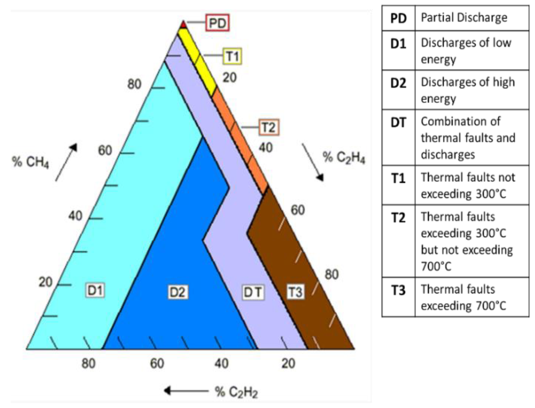
Duval Triangle Method: This is a graphical method developed by Duval to analyze DGA data using three gases, CH
4, C
2H
2, and C
2H
4, which are plotted along three sides of a triangle as shown in
Figure 1 [
13]. The triangle is divided into seven zones, indicating various transformer faults including partial discharge, thermal faults at various temperatures, and electric arcing. While the Duval triangle provides more accurate diagnoses than the above ratio methods, it does not encompass a fault-free zone; hence, this method cannot be used to detect incipient faults.
As can be seen from the above discussion, all existing DGA interpretation techniques comprise shortcomings that make them unreliable to some extent. As such, DGA must be conducted and analyzed by expert personnel. This makes the DGA interpretation process inconsistent and different conclusions may be reported for the same oil sample if analyzed by different personnel. This inspired researchers to develop artificial intelligence-based techniques for DGA interpretation, including fuzzy logic [
14], which is also employed to identify transformer criticality and remnant life based on DGA data [
15,
16], neural network [
17], gene expression programming [
18,
19], support vector machine [
20], and particle swarm optimization [
21]. While AI-based DGA interpretation techniques published so far in the literature provide more reliable diagnoses than the conventional interpretation methods, they fail to diagnose some faults in oil and cellulose, and engineering judgment is still required [
22].
2. Proposed DGA Machine Learning Technique
Logistic regression is widely employed in many applications to improve machine learning approaches, as it is suitable for systems of discrete and historical data such as DGA [
23]. As the logistic regression is a method for classifying data into discrete outcomes, it is an ideal method for DGA applications. In supervised learning algorithms, overfitting is a likely problem with many input features. In un-regularized models such as fuzzy logic models, tuning is mainly conducted through training-error minimization. On the other hand, regularized logistic regression methods are widely used to solve problems with numerous features [
24]. In these methods, the outcomes are classified using a cost function that is solved by logistic regression [
25]. The regularization helps to avoid over-fitting due to either small number of training samples or large number of features, and it is often used for proper feature selection by filtering out irrelevant features [
26].
Some algorithms employ conditional maximum entropy models such as the generalized iterative scaling (GIS) [
27]. However, this algorithm is considered as one-sided Laplacian prior which can be extended towards the regularized logistic regression. Another AI-based technique is called grafting, which consists in steadily constructing a subclass of the parameters [
28]. Moreover, the generalized LASSO is an algorithm developed based on the regularized least squares problem [
29].
This paper is taking a forward step into the development of reliable and automated DGA interpretation techniques that can be continuously enhanced through self-learning processes based on historical and future DGA data. One of the cutting-edge techniques of artificial intelligence is deployed to understand the DAG data through machines without the need of human intervention. The regularized logistic regression is implemented based on the iteratively reweighted least squares (IRLS). The technique utilizes a one-vs-all method in order to analyze and then classify DGA data into one fault out of a set of possible transformer faults.
Regularized logistic regression is a distinguished tool utilized in machine learning. The proposed algorithm is designed to classify the condition of DGA oil samples automatically into designated faults. Classified faults include partial discharge (PD), low and high energy discharge (D1 and D2, respectively), and low, medium, and high thermal faults (T1, T2, and T3, respectively). DGA measurements are defined based on five features that are used as inputs to the proposed machine learning algorithm. DGA results, including H
2, CH
4, C
2H
6, C
2H
4, and C
2H
2 are fed into the algorithm as a percentage of the total concentration of these gases (gas-ratio). The proposed model is developed using 446 DGA samples collected from the literature and Egypt electric utilities, and are divided into two sets. The first set (335 samples) is used for training processes including model validation (67 samples), while the second set (111 samples) is used for testing the developed model.
Table 6 shows the actual fault classifications of the collected 446 DGA samples.
The proposed model is based on a regularized supervised learning approach in which all data are labelled. The number of labelled samples used in this model is given by . Each collected sample is represented by x and y coordinates that represent the input and output, respectively. Each input is represented as an N-dimensional vector that represents the input feature vector of the DGA five-gas ratios. Moreover, each output is a class labeled that represents one of the possible six fault types mentioned above.
As shown in
Figure 2, the data preparation stage includes two steps: data normalization and samples shuffling. In the first step, the collected samples are normalized to ensure the input features (DGA measurements) have fair influence on the output. In the second step, the collected samples are shuffled to remove any undesired pre-order effects.
After the preparation stage, the collected samples are divided into three sets as follows:
- (1)
The training set, consisting of 268 samples or 60% of the entire data set, is utilized to form the initial model;
- (2)
The validation set, consisting of 67 samples or 15% of the entire data set, is utilized to optimize the regularization parameter () to form the final model;
- (3)
The testing set, consisting of 111 samples or 25% of the entire data set, is utilized for testing the final model.
It is worth mentioning that while data splitting is performed randomly, all data classes, i.e., all fault types, are included in each data set. The percentages of data sets were chosen based on the usual practices used in the literature [
30].
For each output class
, the one-vs-all logistic regression method is used to train a hypothesis classifier
. In this method, the hypothesis calculates the probability of the output corresponding to one of the possible faults, e.g.,
. This process is repeated for all samples to calculate the probability of each fault corresponding to the used DGA sample and the output with the highest probability considered as the classified fault. The cost function for such logistic regression
as a function of model parameters
θ is given by:
The hypothesis classifier defines the probability distribution for each class label
given a feature vector
as follows:
The classifier is trained for each output class by utilizing the training sample set. Therefore, for a given input feature , the algorithm optimizes the classifier to predict a class that maximizes the hypothesis . A developed MATLAB code is utilized to train the classifier by minimizing the cost function .
The first term is always positive since the hypothesis classifier goes only from 0 to 1. The second term in Equation (1) represents the regularization term that is used to avoid model overfitting. This term is optimized using the validation sample set. In Equation (3), all model parameters are penalized with a ratio that minimizes the cost function with the
parameter. After spanning through a range of values for
from 0.001 to 10, the obtained optimum value is
1 as shown in
Table 7 and
Figure 3. The training error is still acceptable at this value while a significant reduction is achieved in the validation error.
The algorithm process goes through three main steps. Firstly, the training sample set is used to train the model and find the model parameter that correlates the input and output factors. Secondly, the validation sample set is utilized to find the proper regularization parameter (). Thirdly, the test sample set is used to test the model which was kept apart from the system modeling to ensure proper independent validation.
3. Results and Nonlinear Approximation
The prediction accuracy (
η) can be estimated as follows:
Using the basic input five features, the algorithm can be used to predict the output fault with an accuracy of 82.9% (
). After initial tuning of the regularization parameter, the system accuracy is slightly increased to 83.8% (
0.01). When the inputs are used as percentages instead of absolute values, the accuracy (for test samples) is improved as can be seen in
Table 8. The polynomial regression shows an increase in the accuracy up to 86%.
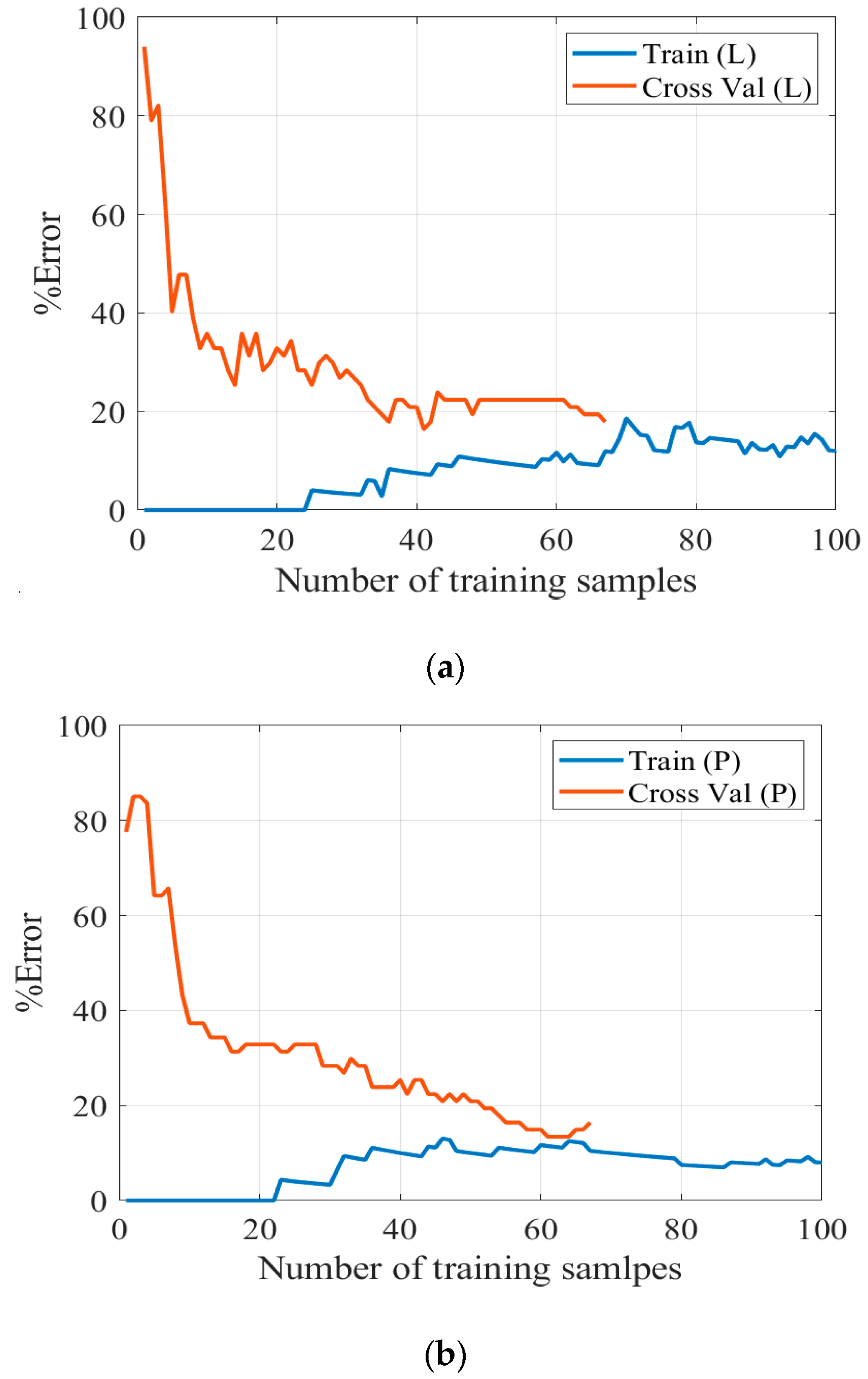
The learning curves with the prediction error (
) for the linear approximation of the proposed model is shown in
Figure 4a. At the beginning, the training set comprises low error since the system can easily approximate the function over very few samples, but as the number of samples increases, the training error also increases but settles at a level of less than 20% when the number of samples increases to 100. On the other hand, the error of the validation set is high when a few samples are used, but it drops as the number of samples increases.
Figure 4a,b show the linear and polynomial learning profiles for the logistic regression; respectively. The error results shown in this figure reveal the nonlinear characteristic of the investigated problem. Hence, it is not accurate to express the system using a linear combination of the features. One way to approximate the nonlinear feature of the investigated problem is through using polynomials. As noticed, by increasing the number of samples, the cross-validation error decreases. Moreover, the training error curve shows that the model is biased and, therefore, additional features are required where the nonlinear combination of features is considered. To select an optimum polynomial order,
p is changed in the range 4–12 and the number of features along with the corresponding error are recorded in
Table 8. It can be seen that for
p = 8, the lowest percentage error is obtained. For values of
p above 8, the error increases, again showing an overfitting problem at
p = 10.
The regularization term is more prominent when the number of features increases as in the polynomial features case. The total number of features for 8th order polynomial (
) with five independent variables (
) including homogeneous
and nonhomogeneous
terms is calculated as follows:
The nonhomogeneous term is given by and hence the total reaches 320 features.
Results of the algorithm using the polynomial features can achieve an accuracy of 86%, as shown in the training curve in
Figure 4b. The last column of
Table 9 demonstrates the predicted faults using polynomial features for logistic regression with testing dataset samples.
Table 10 presents a summary of the obtained results for each fault using the testing dataset (111 samples). In order to highlight the system capability to detect various faults using DGA results, the predicted fault types using polynomial regression are compared with the actual faults. Results attest the capability of the proposed model in detecting different fault types, especially low and high thermal faults (T1 and T3) with a high degree of accuracy. As can be seen in
Table 10, the overall prediction accuracy of the testing samples is 85.6%.


 ,
, 

