The data used in this study took into account three different datasets. Dataset one was related to energy consumption while the second dataset described the volume of the flow of water at the entrance of a WWTP. The third dataset described the climatological conditions. The first two datasets were made available by a Portuguese wastewater company and were related to a single WWTP. Regarding the energy consumption value, which is the target feature, there is an intrinsic relationship between the different processes present in a WWTP and the required energy (typically, the larger the WWTP, the greater its energy consumption). However, this relation was captured and described in the time series in itself as the values were a snapshot of the state of the WWTP. The third dataset was collected using the Open Weather Map API, and contains climatological data regarding the same city where the WWTP was located. All datasets contained observations belonging to the period between January 2016 to May 2020.
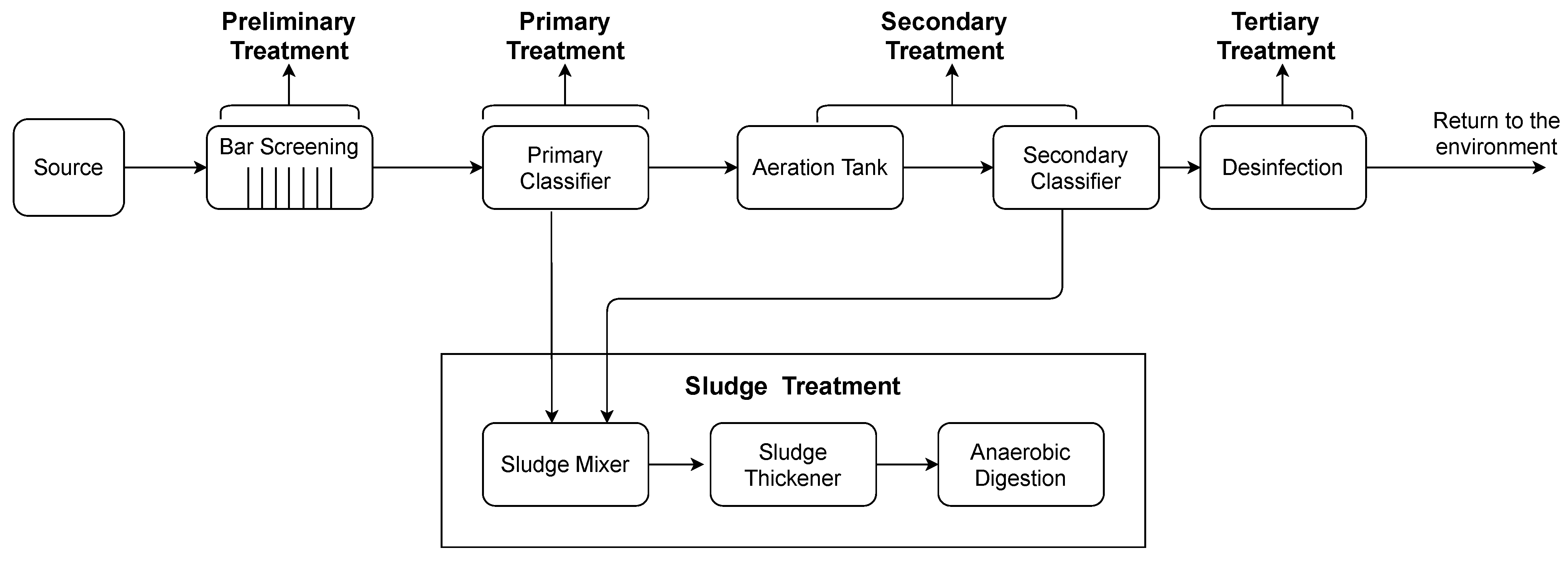
Figure 1 illustrates the WWTP layout used in this study. This WWTP was based on four main stages: preliminary, primary, secondary and tertiary treatments. In addition, there was also a line responsible for the sludge treatment. The preliminary treatment, which included bar screening, was accountable for removing solids and materials of greater volume, an essential step in the WWTP process since some of these objects could damage some equipment in the following steps. The primary treatment, which included the primary classifier, aimed to remove the smaller volume solids, namely the suspended solids, from the previous stage and the organic matter present. In the secondary treatment, two processes were included, the aeration tank and the secondary classifier. This stage aimed to remove biodegradable organic matter from wastewater, in addition to suspended solids and nutrients, such as nitrogen. Finally, the tertiary treatment was responsible for removing the remaining suspended solids resulting from the previous stages. The sludge produced in the primary and secondary treatment was inserted in the sludge treatment line. This line was responsible for dewatering and disinfecting the sludge, reusing it as an energy source.
2.1.1. Data Exploration
The energy consumption dataset comprised two features: the energy consumption value (in kWh) and the corresponding timestamp, making 1522 records with a daily periodicity. The influent flow dataset also contained two features, i.e., the value of the influent flow (in m
) and the timestamp, with a total of 1535 records, again with a daily periodicity. Finally, the climatological dataset had a total of 25 features, including the timestamp, air temperature, and humidity, among others, with a total of 38,651 hourly timesteps.
Table 1 presents the different features available in the three datasets, detailing its characteristics and presenting the corresponding units of measure.
None of the three datasets had missing values. However, as in its genesis the problem identified in this study was based on a time series problem, it was essential to pay attention to missing timesteps. In the case of the climatological dataset, there were no missing timesteps. On the contrary, both the energy consumption and the influent inflow datasets contained missing timesteps. In the former, there were 88 missing timesteps, while in the latter 75 missing timesteps were identified. In a subsequent section, it is explained how to overcome the missing timesteps problem.
As the main goal of this study was to forecast energy consumption, data exploration emphasized the value_energy feature of the energy consumption dataset. Firstly, it is worth mentioning that this feature presented an accumulated value. Hence, it was necessary to subtract, from each observation, the value of the previous one, in order to obtain its real value. Since the first observation had no previous one, it was removed. A box plot analysis allowed us to identify the existence of some extreme outliers that were derived from an incorrect insertion of values by the operators of the WWTP.
A statistical analysis of the energy consumption values was performed, being described in
Table 2. It was possible to verify that the mean energy consumption value in the dataset presents a value of 8050.96 kWh, with a standard deviation of 3736.359 kWh. The skewness was 3.172, representing an asymmetric distribution, i.e., the positive value indicates a positive inclination in the distribution of the data, in which the tail size of the right hand is larger than that of the left. Regarding the kurtosis value, it was 28.101. A kurtosis value greater than 1 indicates that the distribution of energy consumption has a very high peak (a leptokurtic distribution).
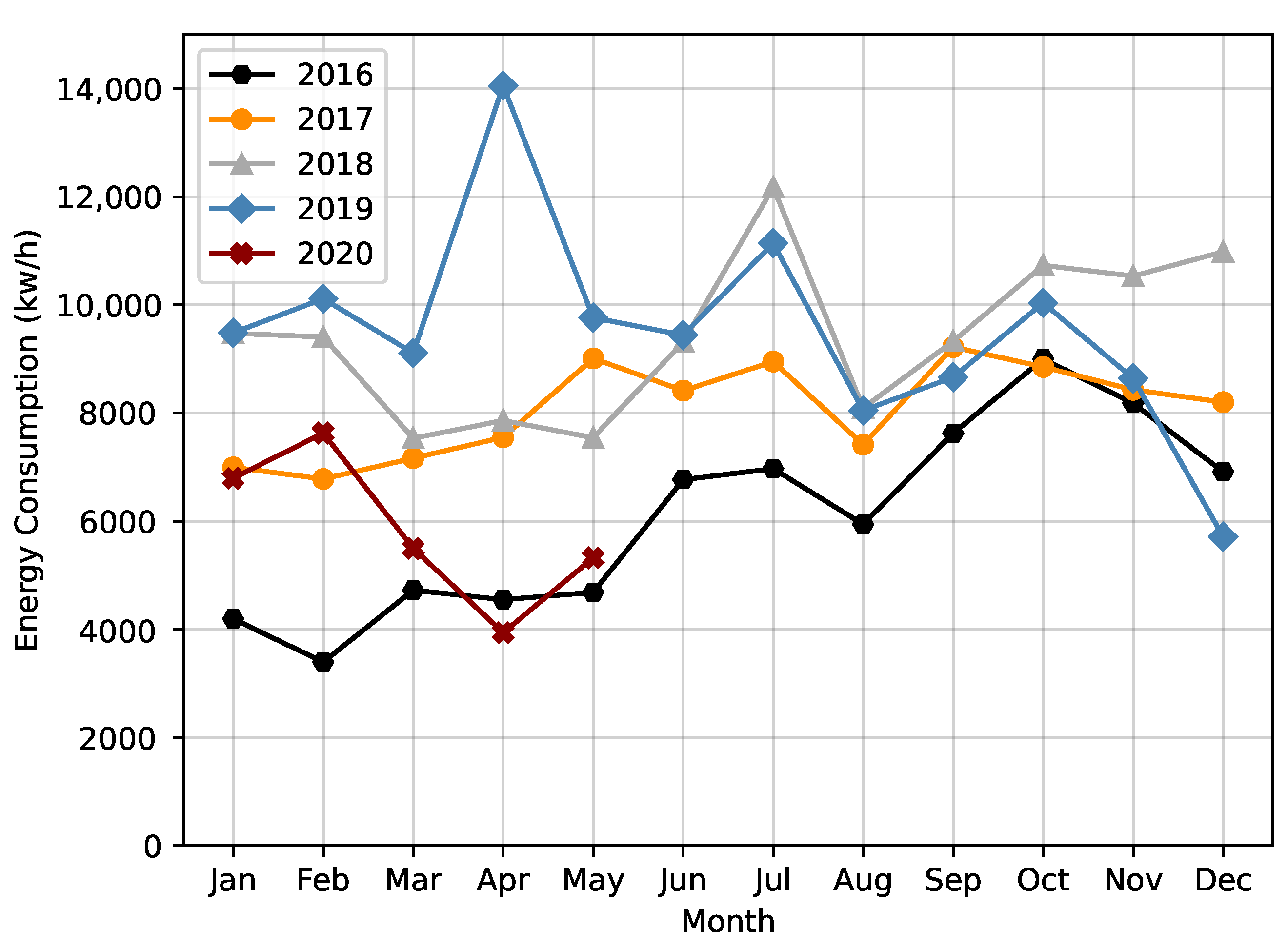
We then explored the energy consumption over the months of a year, during the 5 years present in the dataset. In
Figure 2 it is possible to verify a pattern in all the explored years, with a constant drop in energy consumption between July and August.
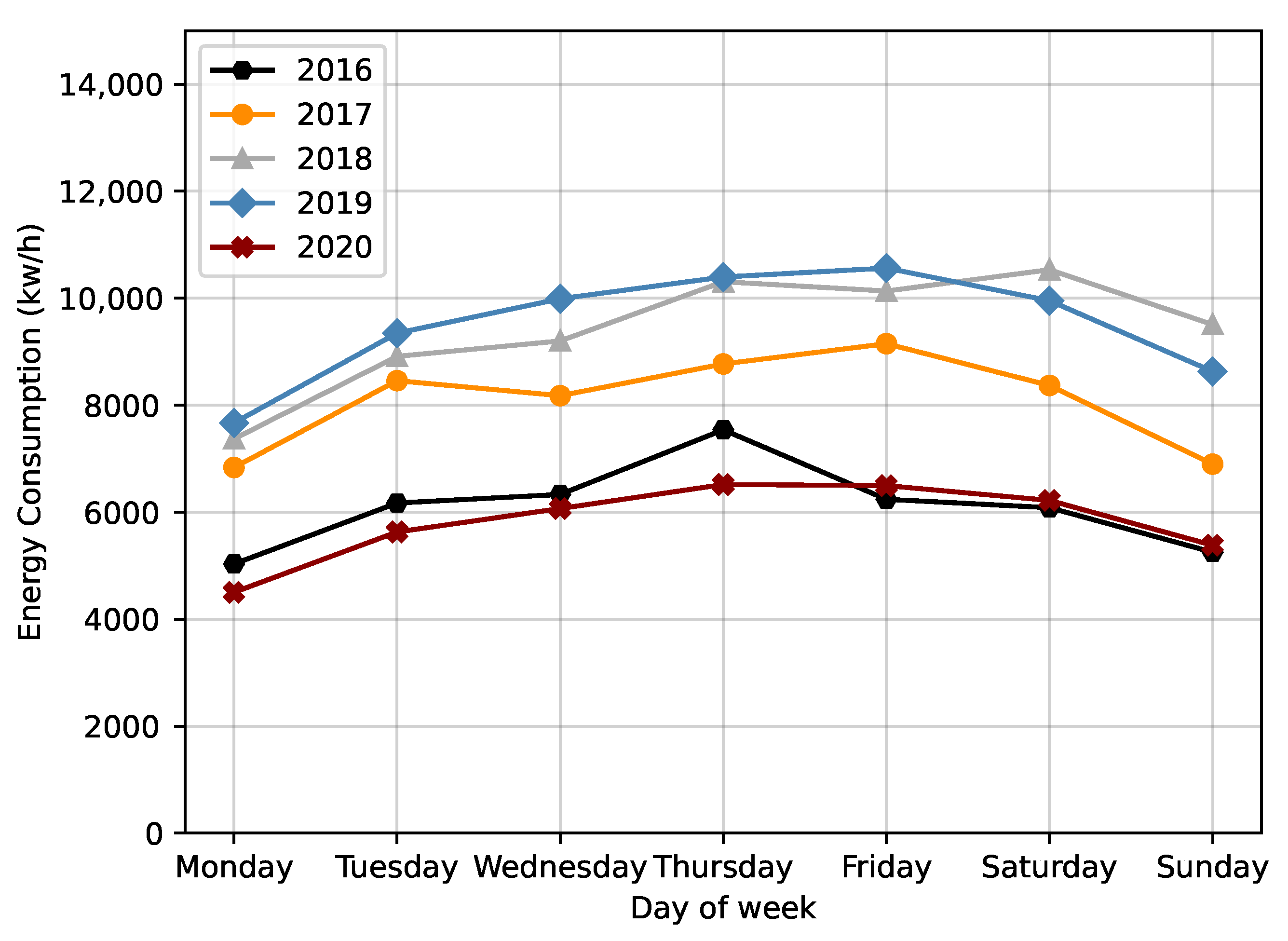
Another analysis took into account the variation in energy consumption over the different days of the week. This analysis was based on the mean value of the days of the week for each year. As shown in
Figure 3, it is possible to verify that Sunday and Monday were the days when there was less energy consumption in the WWTP. In conclusion, it appears that the traditional working days had a higher energy consumption on average, while on weekends there was a decrease.
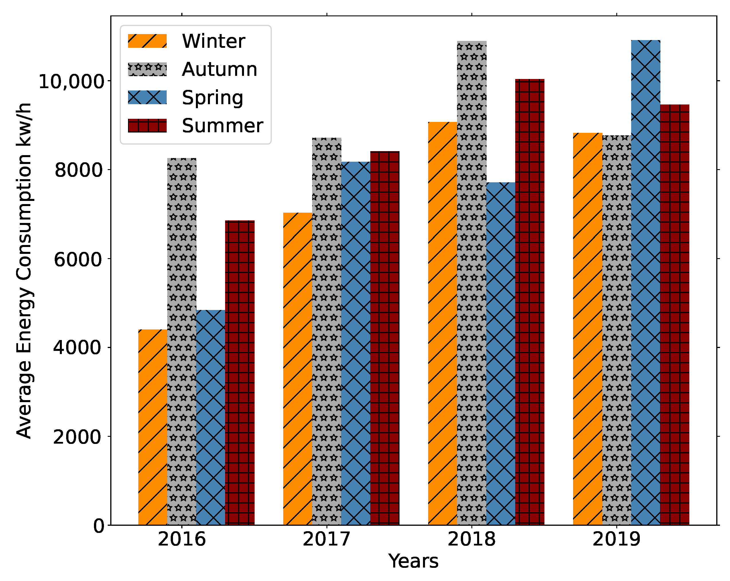
To understand seasonality, we performed two different analyses on the energy consumption data between 2016 and 2019: the first relative to the average consumption by season and the second related to the energy consumption per trimester.
Figure 4 depicts the first analysis, being possible to verify that, typically, more energy was consumed during the autumn. Interestingly, in 2019, autumn was the season with the lowest average energy consumption value. In general, it was also possible to see that over the years, energy consumption was rising in different seasons. Despite a higher number of average consumption values, it was not in the autumn that the highest average peak was reached, but in the spring of 2019 with a value of 10,912 kWh. Regarding the lowest peak, it occurred in the winter of 2016, with a value of 4398 kWh. Additionally, it was possible to verify that, in general, winter was the season with less consumption of energy.
The trimesters analysis showed that the fourth trimester had the highest energy consumption values over the first three years. Despite this, the highest value was verified in the second trimester of 2019, with 11,072 kWh. As demonstrated in the seasons’ analysis, in general, the average values increased during the first three years. In 2019, there was an increase in the first and second trimester and a decrease in the third and fourth ones.
Regarding the influent flow, an analysis was carried out considering the average for each year, described in
Table 3. As can be seen, 2019 was the year with the highest volume of influent flow on the WWTP (1155.33 m
). Interestingly, checking the year of 2019 concerning the energy consumption (
Figure 2), we verified that this year also obtained, in general, the highest average of energy. On the other hand, looking at 2016, excluding the incomplete year of 2020, this was where the lowest average influent flow value occurred, this being, in general, the year with the lowest energy consumption value.
2.1.2. Data Preparation
The first step to prepare the data were to carry out a feature engineering process in the three datasets, thus creating three new features from the timestamps (i.e., year, month, and day). The dataset related to climatological data, as mentioned, had an hourly periodicity, so to match the same periodicity as the other datasets, these were grouped by day, month and year, aggregating the mean value per feature.
As referred above, as both the energy consumption and influent flow datasets presented accumulated values, a method was applied to obtain the value that would correspond to each specific day. The identified extreme outliers, which corresponded to miss insertions of values by the operators of the WWTP (for example, extra digits), were also solved. The remainder of the data treatment is specified in the following lines.
Handling Missing Timesteps
To deal with the missing timesteps verified in the energy consumption and the influent flow datasets, a dataset was created comprising all days (i.e., timesteps) that should have been present in the dataset. In both cases, the start date was 2nd January 2016 and the end date 28 May 2020. The datasets were joined, with missing timesteps being added and having its features filled with the −99 value. Solving the missing timesteps problem created a new one, missing values, i.e., timesteps that were missing were now present but all their features had the −99 value.
Handling Missing Values
To fill the missing values, a queue-based approach was followed. Each record was read for each of the two datasets with missing values, saving its value (energy consumption or influent flow) in the mentioned structure, with a maximum size of eight values. Whenever reading a record, if the queue was full, a push operation would be performed at the beginning of the queue. When a timestep had a feature with the −99 value, its value would be computed based on the average of the last eight records, i.e., the previous 8 days, present in the queue. Once calculated, this value would then be pushed to the queue, eliminating the oldest record. By the end of this process, no dataset had missing values neither missing timesteps.
Joining Datasets
When reaching this point, each one of the three datasets was made of 1609 observations. However, we were required to join the three datasets into a single one. This was performed using the features year, month, and day. In the end, a single dataset was created, having 1609 observations with 30 features each.
Correlation Analysis
To verify which features had a more significant correlation with the target feature (
value_energy), it was first necessary to check whether the data followed a normal distribution. Using a
and the Kolmogorov–Smirnov test, it was possible to verify that all features assumed a non-Gaussian distribution. Hence, it was necessary to use the non-parametric Spearman’s rank correlation coefficient, being possible to verify that the features that had a more significant correlation with the target were the year, month, temperature, and
flow_value. Since the other features had a low correlation with the target, they were removed. After this treatment, the final dataset had 1609 observations with a shape (1609, 5).
Table 4 shows an example of a record in the final dataset.
Handling Outliers
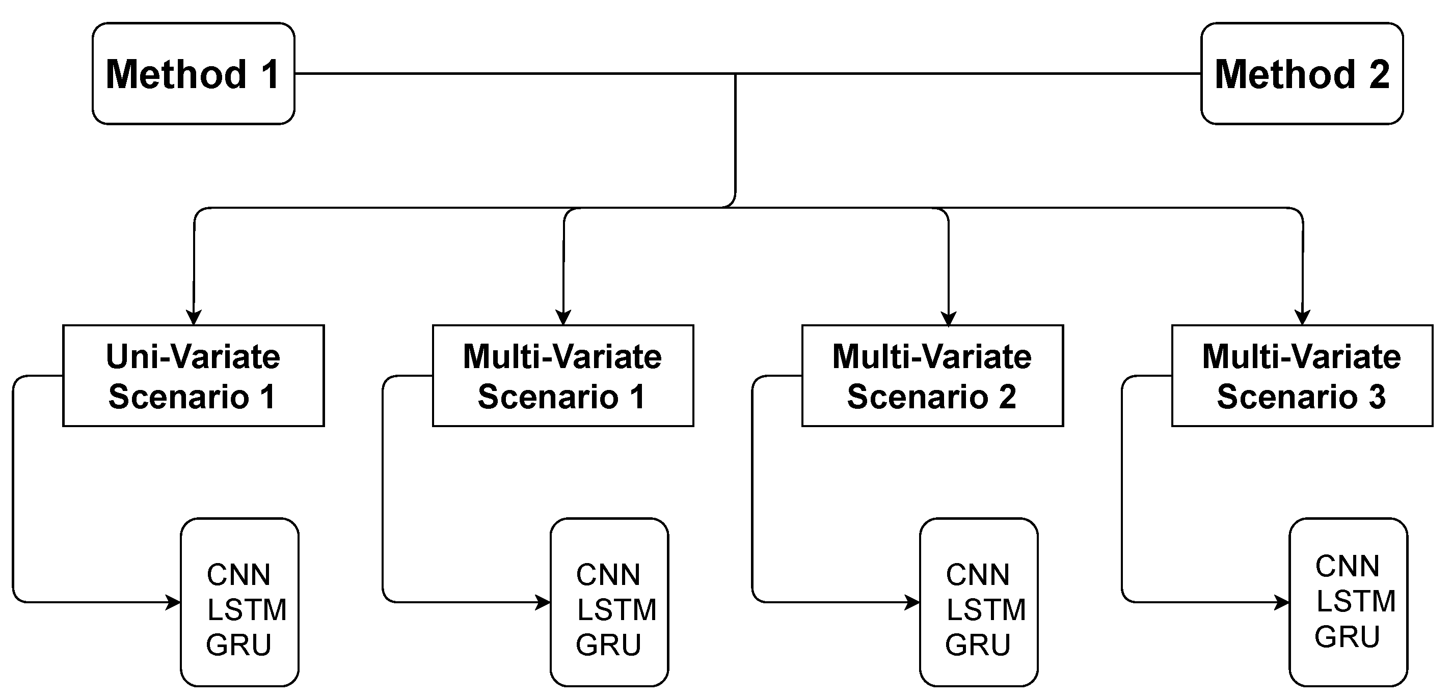
Extreme outliers were above 14,000 kWh. Only six observations were below 2000 kWh. Since the range between the maximum and minimum values for the feature value_energy was large, and considering the reduced amount of observations that were causing it, two different methods were experimented to handle outliers. These two methods provided a comparative term for the different experiments, causing slight modifications to the input data that were fed to the models. The two methods were as follows:
Method 1—to further reduce the amplitude of the target feature, the few timesteps with value_energy greater than 10,000 kWh or lower than 2000 kWh had their value updated, using the queue-based approach described above. The goal was to use interpolation to replace the outliers;
Method 2—to further reduce the amplitude of the target feature, the few timesteps with value_energy greater than 10,000 kWh or lower than 2000 kWh had their value truncated. The goal was not to use interpolation to update the target value.
Normalisation
With the data prepared, the next step was to normalize them. Since LSTMs work internally with the hyperbolic tangent, we decided that the applied normalization would be in the range [−1, 1], according to the following equation:
Supervised Problem
The final step was to go from an unsupervised problem to a supervised one, with the respective inputs (X) and corresponding labels (y). Thus, it was necessary to create sequences of data, which depend on the number of timesteps used as input for the models. A sliding window was used over the initial dataset to create the different sequences and the respective labels, thus creating a set of sequences that can be fed to the models. As an example, if the shape of a model’s input was (1601, 7, 5), the first element set the number of samples, the second the number of input timesteps, and the last the number of features. In this example, the labels would have the shape (1601, 1). A similar algorithm can be seen in the work of Fernandes et al. [
15].


