A Review of Plant Phenotypic Image Recognition Technology Based on Deep Learning

Abstract

Plant phenotypic image recognition (PPIR) is an important branch of smart agriculture. In recent years, deep learning has achieved significant breakthroughs in image recognition. Consequently, PPIR technology that is based on deep learning is becoming increasingly popular. First, this paper introduces the development and application of PPIR technology, followed by its classification and analysis. Second, it presents the theory of four types of deep learning methods and their applications in PPIR. These methods include the convolutional neural network, deep belief network, recurrent neural network, and stacked autoencoder, and they are applied to identify plant species, diagnose plant diseases, etc. Finally, the difficulties and challenges of deep learning in PPIR are discussed.

1. Introduction

Plants are indispensable resources that are present on the earth. They play an important role in the development of the society and they have great significance in environmental protection, medical pharmaceutical, agricultural development, and food-related applications [1]. However, any plant-related work, such as plant species and diseases identification and evaluation of plant production, is becoming increasingly complex. An important starting point for any plant-related work is the identification of plant phenotype that refers to the physiological and biochemical characteristics of plants, including their color, shape, texture, and so on, which are determined by both genes and the environment. Traditional methods of plant phenotype identification include artificial identification, phytochemical classification, the anatomical method, morphological method, and genetic method, which are difficult to implement, have low efficiency, and unstable accuracy [2]. With the development and popularity of computer technology, image recognition technology is becoming increasingly mature, and it has been successfully applied in many fields, such as face recognition, object detection, medical imaging, etc. [3,4]. Plant phenotype identification tht is based on image processing technology has become a popular topic of research, leading to new breakthroughs and improved accuracy. In particular, deep learning has been proposed in order to further promote the development of PPIR [5]. Table 1 shows recent relevant reviews.

Table 1. Recent relevant reviews.

References	Review Main Points
Muhammad et al. [6]	This paper aims to review and analyze the implementation and performance of various methodologies (artificial neural network (ANN), probabilistic neural network (PNN), convolutional neural network (CNN), K-nearest neighbor (KNN) and support vector machine (SVM)) on plant classification. At the same time including feature extraction and preprocessing technology. Each technique has its advantages and limitations in leaf pattern recognition. The quality of leaf images plays an important role, and therefore, a reliable source of leaf database must be used to establish the machine learning algorithm prior to leaf recognition and validation.
Weng et al. [7]	In this survey, authors elaborate the wor k from four different aspects: (1) plant morphology and physiological information extraction, (2) plant identification and weed detection, (3) pest detection, and (4) yield prediction. It focuses on the specific application of convolutional neural networks in this field. Authors also analyze the pros and cons of these methods compared to traditional approaches. The potential future trends of plant phenotyping research are discussed at the end of this survey.
Wang et al. [1]	The review introduces the research significance and history of plant recognition technologies. Then, the main technologies and steps of plant recognition are reviewed. At the same time, more than 30 leaf features (including 16 shape features, 11 texture features, four color features), and then SVM was used to evaluate these features and their fusion features, and 8 commonly used classifiers are introduced in detail. Finally, the review is ended with a conclusion of the insufficient of plant identification technologies and a prediction of future development.
Barbedo [8]	This paper provides an analysis of each one of those challenges, emphasizing both the problems that they may cause and how they may have potentially affected the techniques proposed in the past. Some possible solutions capable of overcoming at least some of those challenges are proposed. Focusing on plant diseases, automatic identification, visible symptoms, digital image processing, extrinsic factors (image background, image capture conditions), intrinsic factors (symptom segmentation, symptom variations, multiple simultaneous disorders, different disorders with similar symptoms), other challenges and future prospects.
Cope et al. [9]	The authors review the main computational, morphometric and image processing methods that have been used in recent years to analyze images of plants, introducing readers to relevant botanical concepts along the way. They discuss the measurement of leaf outlines, flower shape, vein structures and leaf textures, and describe a wide range of analytical methods in use. At last, they discuss a number of systems that apply this research, including prototypes of hand-held digital field guides and various robotic systems used in agriculture. They conclude with a discussion of ongoing work and outstanding problems in the area.
Waldchen et al. [10]	This paper is the first systematic literature review with the aim of a thorough analysis and comparison of primary studies on computer vision approaches for plant species identification. They identified 120 peer-reviewed studies, selected through a multi-stage process, published in the last 10 years (2005–2015). After a careful analysis of these studies, they describe the applied methods categorized according to the studied plant organ, and the studied features, i.e., shape, texture, color, margin, and vein structure. Furthermore, they compare methods based on classification accuracy achieved on publicly available datasets. Their results are relevant to researches in ecology as well as computer vision for their ongoing research.
Thyagharajan et al. [11]	Authors review several image processing methods in the feature extraction of leaves, given that feature extraction is a crucial technique in computer vision. As computers cannot comprehend images, they are required to be converted into features by individually analyzing image shapes, colors, textures and moments. Images that look the same may deviate in terms of geometric and photometric variations. In their study, they also discuss certain machine learning classifiers for an analysis of different species of leaves.
This paper	In this paper, three categories of plant image recognition algorithms are summarized, and the methods of plant image preprocessing and plant image feature extraction are summarized. Then, the advantages and disadvantages of imaging technologies are explained. At last, the specific applications of four common deep learning models in plant image recognition are described.

2. PPIR Technology

2.1. State of the Art in PPIR Technology

The development of PPIR technology started several decades earlier internationally, focusing on feature extraction and training of plants using traditional methods. In the 1980s and 1990s, Ingrouille et al. [12], from the University of London, extracted 27 main characteristics of plant leaves and used principal components analysis (PCA) in order to classify oak trees. Yonekawa et al. [13], from the University of Tokyo, fused several prominent features of plant phenotypes, such as texture, color, and shape for image recognition, and used the backpropagation (BP) neural network algorithm to train and classify image data. In 2006, Cheng et al. [14] used fuzzy functions for shape matching and identification of plant phenotypes. CLEF 2011–2015 (Cross Language Evaluation Forum) in the BBS held pictures of plant classification of image recognition under acomplex environment; the library has 1000 kinds of plant species. Villena et al. [15] utilized scale invariance to extract plant phenotypic traits that can be identified. In 2013, Charles et al. [16] established a database of 100 plants containing 16 samples for each plant, carried out feature extraction, and proposed a high-accuracy recognition algorithm under the condition of small training set size, based on the k-nearest neighbor (KNN) algorithm. When the shapes, textures, and edges of the plant phenotypes were fused, an accuracy of 96% was achieved.

The research on PPIR started late domestically, but it is worth learning from. In 2007, Wang et al. [17] used a moving center hypersphere classifier to classify eight geometric features and seven image invariant moments that were extracted from ginkgo leaves with an accuracy rate of 92%. In 2009, Wang et al. [18] extracted the feature vectors of maize leaves while using morphology and contour extraction, and then classified them while using the genetic algorithm for optimized selection of the features. Subsequently, Fisher’s discrimination method was used in order to identify the diseased leaves with an accuracy rate of more than 90%. In Reference [19], Zhai et al. used the relational matching structure method to match the plant leaves images and different model structures after feature extraction, and identified the types of plants based on the matching level. In 2015, Wang et al. [20] proposed a plant leaves fusion-based recognition system to extract the development characteristics of a variety of foliage plant phenotypic traits, such as shape, color, texture, leaf margin, etc. Support vector machine (SVM) classification was used for plant identification, and the experimental results showed that an accuracy of 91.41% was achieved while using the SVM, which was better than that with a BP neural network or the KNN algorithm. In spectroscopy, Cen et al. [21] used hyperspectral imaging technology in combination with supervised classification algorithm for cucumber freezing damage detection, selected and compared the best band in the experiment, and finally adopted three algorithms of naive bayes, SVM, and KNN for classification; the results showed that the accuracy was higher than 90%, showing the outstanding potential of hyperspectral imaging technology in plant disease detection.

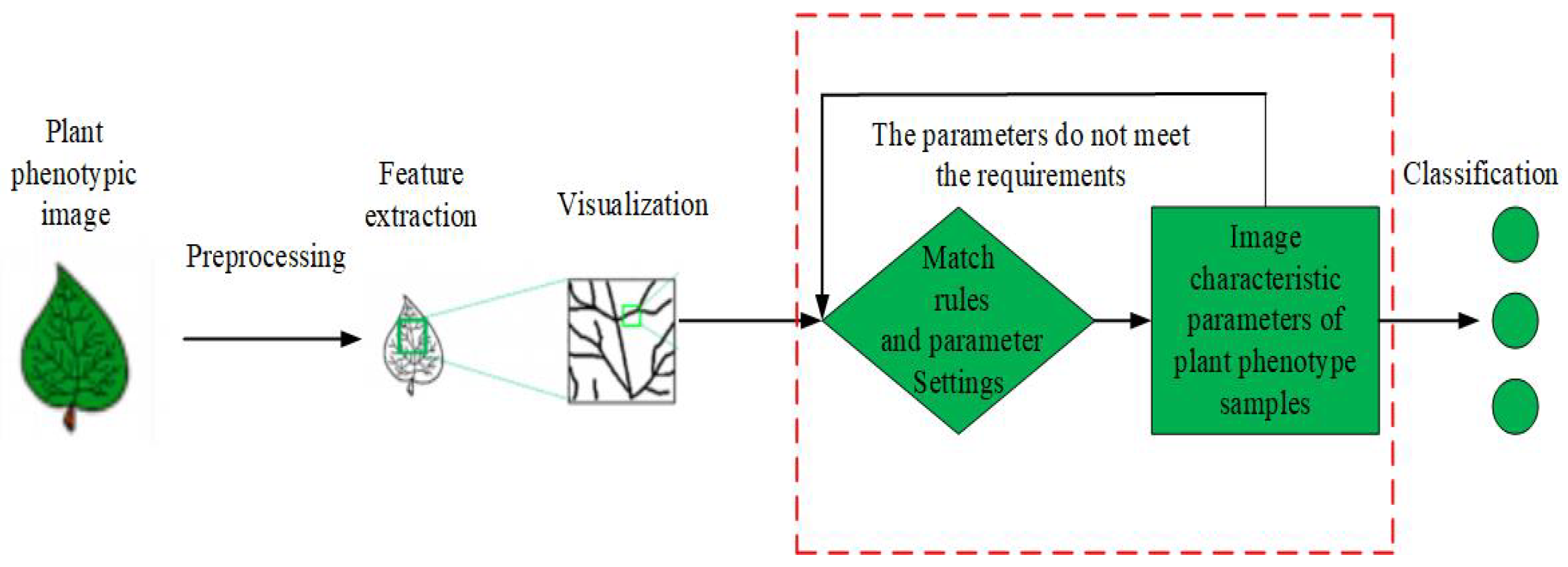
2.2. Traditional PPIR Techniques

The existing PPIR methods can be mainly divided into three categories [3], which are described, as follows:

(1) the basic idea of relational structure matching method for PPIR is shown in Figure 1 [22]. In this method, first, the input images are preprocessed in order to extract features, while using multi-scale curvature space to describe the geometric features, as well as the fuzzy particle swarm algorithm and genetic algorithm. Second, the algorithm matching rules and parameters are set. Finally, the extracted features are matched with the features from the sample database and images are classified based on the matching degree [23,24].

Figure 1. Flow chart of relational structure matching method.

(2) PPIR that is based on mathematical statistics is the most widely used method. Figure 2 shows its basic idea. First, a mathematical model is set up, followed by quantitative analysis and classification of the image. The methods in this category are based on Bayesian discriminant functions, KNN, kernel PCA, Fisher discriminant method, etc. [25,26,27].

Figure 2. The flow chart of mathematical statistics methods.

(3) Traditional machine learning-based PPIR mainly consists of artificial neural network, moving center hypersphere classifier, SVM, etc. [28]. Machine learning refers to a set of computerized modeling methods whose patterns are learned from data in order to automatically make decisions without explicit rules. The main idea of machine learning is to make effective use of experience or sample scenarios to discover the underlying structure, similarity, or difference in the data, so as to correctly interpret or classify new experience or sample scenarios [29]. It is important for programers to deploy specific machine learning approaches to their specific problems to make informed choices. The application of plant phenotype can be summarized into four aspects: (a) identification and detection, (b) classification, (c) quantification and estimation, and (d) prediction. In addition, data preprocessing steps, such as dimensionality reduction, clustering, and segmentation, can also be the key to a successful decision [29]. The moving center hypersphere classifier considers the sample points of plant phenotypic image data as a series of hyper spheres. A set of sample points are considered to be part of a hyper sphere, whose radius is expanded to include as many sample points as possible [26]. The SVM is a supervised learning model that is applicable to linearly or nonlinearly separable and a small number of samples. The method can be extended to high-dimensional pattern recognition by projecting the data points into a higher dimensional space and computing a maximum-margin hyperplane decision surface [26]. The SVM can be used to classify the plant phenotypic image data. Figure 3 shows its basic idea.

Figure 3. Flow chart of support vector machine (SVM).

Feature extraction involving the extraction of shape, texture, color, and other major feature information is an important step in PPIR [22]. In shape based feature learning, edge detection and shape context description methods are widely used in order to extract the plant contours from the input images to achieve plant recognition [19]. Texture-based feature learning includes internal information of plant phenotypes and, generally, it is based on a local binary pattern (LBP) algorithm that calculates the correlation between a pixel and its surrounding pixels in an object [24]. Color based feature learning is more stable and reliable when compared with the aforementioned learning methods. It is robust and not sensitive to the target size and orientation of the color characteristics. It usually uses the percentage of pixels of different colors in red, green, and blue (RGB), or hue, saturation, and brightness (HSV) images, and their histograms for feature extraction and image recognition [25]. These feature learning methods focus on the attributes of plant phenotypes and they mostly include shallow learning methods that need manual feature extraction.

At present, a variety of imaging technologies are used in order to collect complex traits that are related to growth, yield, and adaptability of biotic or abiotic stresses (such as disease, insects, drought, and salinity). These imaging technologies include visible light imaging (such as machine vision), imaging spectroscopy (such as multispectral and hyperspectral remote sensing), thermal infrared imaging, fluorescence imaging, 3D imaging and tomography (such as positron emission computer tomography), and image and computer tomography). Many institutions and organizations in the world have carried out phenotypic group analysis, such as the Australian plant phenomics facility. At the same time, there are also some high-throughput phenotypic testing platforms that are deployed in the field or indoors, such as LemnaTec. Although phenotype analysis of plants that is based on optical imaging has many advantages, it also faces some difficulties. For example, when machine vision methods are used to process visible light images in order to obtain phenotypic information, such as plant species, fruit quantity, and pest categories, it is difficult to resolve adjacent leaves problems, such as overlap and occlusion that are caused by ears and fruits. Images that were collected in a laboratory environment often have a pure background, uniform lighting, and a small number of plants or organs contained in the image. Solving practical problems in the field is often caused by complex backgrounds, differences in lighting, and occlusion. The interference of object shadows.

For PPIR, especially for a large database of plant phenotypic images, the performance of shallow and single feature learning methods is not satisfactory due to the low recognition accuracy and several interference factors [26].

In Table 2, the advantages and disadvantages of traditional methods that are used for plant phenotypes image recognition are compared.

Table 2. Comparison of traditional plant phenotype recognition techniques.

Methodsand Techniques	Introduction	Advantages	Disadvantages
K-NearestNeighbor (KNN) [22]	KNN algorithm is a basic classification and regression method. In the field of plant phenotype recognition and classification, it mainly undertakes the tasks of feature information retrieval, clustering, information filtering, and species recognition.	1. Simple algorithm and mature theory. 2. Robust with regard to search space. 3. No training is required, confidence level can be obtained.	1. High memory and computational cost at testing stage. 2. Sometimes sensitive to noise or nonlinear input. 3. lazy learning.
ProbabilisticNeural Network (PNN) [16]	The PNN algorithm is a neural network model based on statistical principles. It is a parallel algorithm developed based on the Bayesian minimum risk criterion. Unlike the traditional multi-layer forward network, the BP algorithm needs to be used to calculate the backward error propagation. It is a completely forward calculation process and is often used in the task of plant phenotypic image classification.	1. Strong adaptability to noisy input and variable data. 2. Can have multiple outputs.	1. Complexstructure. 2. Susceptible to overfitting.
SupportVector Machines (SVM) [5]	The SVM algorithm is an excellent data mining technology. Its goal is to find the optimal hyperplane to minimize the classifier error. It is widely used in statistical classification and regression analysis. It usually assumes the role of feature classifier in plant phenotype image recognition.	1. Good generalization. 2. Sparsity of the solution and capacity control obtained by optimizing the margin. 3. Strong fault tolerance ability, relatively stable even with training sample deviation.	1. Complex algorithm structure. 2. Slow training speed.
Decision Trees (DT) [27]	The DT algorithm is a tree-like decision diagram with additional probability results. It is a predictive model that intuitively uses statistical probability analysis to represent a mapping between object attributes and object values. In the field of plant phenotype classification and recognition, it often undertakes analysis the task of collecting statistics on plant phenotypic characteristics.	1. Simple to use and easy to understand. 2. Pruning strategy eliminates a large number of weak correlations and irrelevant information to improve efficiency. 3. Fast prediction ability.	Sensitive to subtle changes in the attribute value.
ArtificialNeural Network (ANN) [28]	ANN algorithm is a kind of simulated biological neural network, which is a kind of pattern matching algorithm. It usually used to solve classification and regression problems. It also used in plant phenotype image recognition.	1. Strong robustness and fault tolerance. 2. Complex nonlinear relations can be modeled using one or more hidden layers.	1. Slow convergence speed and high complexity. 2. Possibility of local overfitting.
Random Forest (RF) [30]	In machine learning, RF is a classifier containing multiple decision trees, and its output category is determined by the mode of the category output by individual trees. It often undertakes species classification tasks in the field of plant phenotypes.	1. The algorithm can handle very high dimensional data without feature selection. 2. Fast training speed, and easy to parallelize method. 3. The algorithm has strong anti-interference ability and strong anti-overfitting ability.	1. When the algorithm solves regression problems, it does not perform as well as it does in classification. 2. The internal part of the model is relatively complicated, and it can only be tried between different parameters and random seeds. 3. For small data or low-dimensional, it may not produce a good classification.

3. Deep Learning Technology and Application in PPIR

3.1. The Development of Deep Learning

Deep learning is a special form of machine learning and its early theory appeared in the 1950s. In 2006, a breakthrough in this field was achieved by a Canadian professor and famous machine learning expert Geoffrey Hinton. In Reference [31], Hinton et al. pointed out that a multi-layer neural network architecture has better feature learning and data mining abilities. The authors further explained that the difficulty of network training in deep learning can be overcome by a layer-by-layer parameter optimization. Microsoft, Baidu, Google, and other high-tech groups have invested significant manpower and financial resources in research that is related to deep learning, which has been widely applied in the field of artificial intelligence and it produced significant benefits. The essence of deep learning lies in multilayer learning models with multiple abstract functions and data representations. It greatly improves the performance compared to existing techniques in the fields of pattern recognition and object detection. In deep learning, the internal parameters are optimized layer-by-layer and features in complex, high-dimensional data are mined through the BP algorithm. The quality evaluation of image recognition technology is as follows, (a) the model parameter optimization problem. Image recognition technology that is based on deep neural network requires training a large number of parameters in order to extract image features, which takes up a lot of running time and computer storage memory. Researchers should improve the model structure and increase the time complexity of the model while ensuring the accuracy of image recognition; (b) training data optimization problem. Deep learning network models rely on a large number of training sets for feature extraction, and the training data sets are unbalanced or even missing, which will greatly limit the application of deep learning technology. How to solve the training data problem should be considered in future research directions; (c) improvement of unsupervised learning. For supervised learning algorithms, a lot of manual data annotation is required for training data, which wastes energy. Subsequent research should strengthen the construction of unsupervised learning algorithms in order to solve the problem of data labeling [32,33,34]. In plant phenotypic image recognition, deep learning is different from traditional shallow learning, because the former can select complex and high-dimensional features without manual intervention. Figure 4 and Figure 5 show the shallow network learning model and deep learning model for PPIR, respectively.

Figure 4. Flow chart of shallow network learning.

Figure 5. Flow chart of deep learning.

In the following, four different deep learning-based image recognition frameworks for plant phenotypes are described.

3.2. Convolutional Neural Network Theory and Application in PPIR

The convolutional neural network (CNN) has shown outstanding performance in image and speech recognition [34]. Lecun et al. [35] combined the BP algorithm with CNN, introduced the error gradient into the CNN for training, and proposed the LeNet-5 model. In 2010, Zeiler et al. [36] proposed deconvolutional networks that function similarly to the inverse process of CNN. The authors pointed out that, although the CNN has translation and scale invariant characteristics, it does not have those characteristics for non-strongly symmetric data. In 2019, Yu et al. [37] proposed a multi-feature weighting (MFR-DenseNet) for image recognition, which could automatically adjust feature extraction channels and judge the interdependence between features of each convolutional layer, thus improving the reflection ability of the structure.

At present, the CNN is the most widely used deep learning model for plant phenotypic image recognition, and its performance is better than that of other deep learning models [38,39]. Gong et al. [40] proposed a method for extracting plant phenotypic characteristics by overcoming the defects of the traditional method. This method used the grayscale images directly as input to the CNN for learning and training. Experiments on the Swedish leaf data set showed that this method significantly improved the recognition accuracy, with the accuracy reaching 99.56%. Grinblat et al. [41] applied the CNN to classify white beans, red beans, and soybeans. The use of CNN avoided the use of handcrafted leaf color and shape features that are difficult to obtain and showed that the classification accuracy improved by increasing the depth of the CNN. An accuracy of up to 96.9% was obtained, which was higher than that of other methods that were based on traditional feature recognition. Dyrmann et al. [39] applied the CNN model with residual branch module training for the identification of weed species. It was shown that an accuracy of 86.2% was achieved on data from six different data sets. This accuracy, although not outstanding, showed that the model could be applied to a wide range of images under varying background conditions and provided the basis for more sophisticated PPIR. Song et al. [42] proposed a Mask R-CNN model to screen the plant images with complex backgrounds, extract valuable feature information, and then use it in GoogleNet for learning and training. The experimental results showed that this method effectively improved the accuracy rate when compared with the classical CNN.

The CNN is a local access multilayer neural network that consists of multiple independent neurons in each layer. The network consists of two parts: feature extraction and feature mapping, including convolution, activation, pooling, and fully connected layers. Figure 6 [43] show the structure of a CNN. In PPIR, thanks to the feature extraction ability of the CNNs, the neurons do not need to individually connect to all parts of the input images. Instead, plant phenotypic feature information in the image is directly extracted through weight sharing between each neuron, which effectively improves the operation speed and accuracy [44]. In the process of training and recognizing different plant phenotype images, the CNN does not focus on a single pixel, but extracts blocks from the whole input images through convolution operations, which effectively integrates the feature information and improves the understanding of image data.

Figure 6. Convolutional neural network structure.

The mathematical model of convolutional neural network can be summarized as follows [44]:

$$X_i^m={\Sigma }_{jϵT_i}{X}_j^{m-1}\times N_{ij}^m+h_i^m$$

(1)

In Equation (1), $X_i^m$ represents the $ith$ feature map of layer m, $T_i$ is the image input to the CNN, $X_j^{m-1}$ represents the $jth$ output of layer $m-1$, $N_{ij}$ is the convolution kernel, and $h_i^m$ is the offset of the $ith$ output of layer m; the result of Equation (1) is then processed by the activation function. The above operation extracts different features from the image data and maintains scale invariance. The pooling layer, which can consist of either maximum pooling or average pooling, down samples the data, decreasing the number of training parameters, achieving dimension reduction, avoiding over fitting phenomenon, and reducing the noise.

$$X_i^m=f_{down}\left(X_i^{m-1}\right)$$

(2)

In Equation (2), $f_{down}$ represents the down sampling function. The CNN convolution and pooling operations are repeated according to the pre-defined number of network layers. After that, the processed feature vectors are stacked and classified while using the fully connected layer. Usually, the $softmax$ and SVM classifier functions are used for classification.

The objective of CNN training is to minimize the value of loss function. Its mathematical expression is:

$$L(W,b)=-{\displaystyle \sum _{i=1}^N\sum _{j=1}^K}g\left({\widehat{y}}_i=j\right)log{p}_i^j$$

(3)

In Equation (3), W is the weight, b is the bias, g is the indicator function, and j is the training sample category. If ${\widehat{y}}_i\ne j$, $I=0$, or else ${\widehat{y}}_i=j$, $I=1$. The prediction probability of category j of the training sample i is given by $p_i^j$ and N is the number of training samples. The loss function and its expected values are used in order to calculate the difference between the output of the CNN and the training data, i.e., the residual difference. The parameters of each layer of neurons in the CNN can be optimized and adjusted while using the gradient descent method. In PPIR, image data preprocessing is carried out first, which includes either RGB model or HSV model transformation, followed by image denoising and filtering, segmentation, and the selection of test and training data. The preprocessed data are then passed through different layers of the CNN. The optimization of different parameters and adjustment of the number of layers can also improve the image recognition accuracy [45,46,47,48].

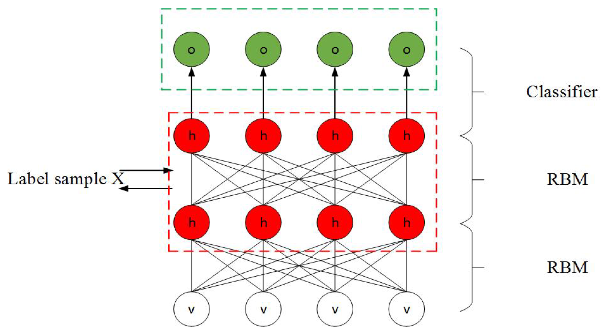
3.3. Deep Belief Network Theory and Application in PPIR

Deep belief network (DBN) is a deep learning model, which was first proposed by Hinton et al. in 2006 [31]. The DBN has shown remarkable performance in areas, such as face recognition and detection, remote sensing image applications, etc. [49]. Jiang et al. [50] combined the DBN and $softmax$ in order to identify text data under a sparse high-dimensional matrix. The authors used the DBN to extract text feature information, applied $softmax$ layer for classification, and used either the gradient descent method or the L-based BFGS (broyden-fletcher-goldfarb-shanno) algorithm in order to optimize the network parameters. The experimental results showed that, with a large amount of data, the proposed method outperformed the SVM and KNN. Fatahi et al. [51] proposed an improved face recognition system that is based on DBN, which increased the recognition rate by enhancing the network structure and optimizing different network parameters. Li et al. [52] classified remote sensing hyperspectral data that are based on DBN and LR (logistic regression), optimized the DBN width during repeated training, and integrated spatial information into the spectral information as the original input, which improved the classification performance by about 15% when compared to the SVM model.

In the field of PPIR, the DBN-based NIR (near infrared spectrum) qualitative model has been applied for plant classification and disease detection, effectively solving high-dimensional and nonlinear problems, and achieving good results. Liu et al. [53] proposed DBN-based leaf recognition that is based on image feature extraction of traditional plant phenotypes and a simple classifier structure. The authors used the “dropout” method in the network training to prevent overfitting, achieving an accuracy of up to 99%. Deng et al. [54] extracted color, shape, texture, and other features of weeds during seedling stage in a rice field, and studied them while using single and double hidden layers. After multi-feature fusion, the features were used as input for training the DBN. An accuracy rate of 91.13% was reached, which was better than that of the SVM and BP models. Yu et al. [55] proposed an alternative to traditional methods of selecting haploid plants with breeding defects and put forward a model that is based on the DBN to identify different varieties of corn haploid that achieved an accuracy of more than 90%. The performance of the proposed model was better than that of the SVM and BPR (Bayesian personalized ranking) models, and the experimental results showed that the network structure of the DBN promoted multitasking learning and information sharing between different varieties. Guo et al. [56] proposed a rice grain blight identification model that is based on the DBN, in which Gaussian filters were used in order to enhance and preprocess the images with diseases, and Sobel edge detection operator was used to extract the disease characteristics. The experimental results showed an accuracy rate of 94.05%, demonstrating the suitability of the proposed model for plant phenotypic disease identification and detection.

The DBN is a special form of Bayesian probability model. In this model, the distribution of input information is generated by a joint probability distribution, and the training data are generated based on the weights of neurons in the model [47]. The neurons in the DBN are divided into two parts: (1) dominant neurons, which receive input information; and, (2) invisible neurons, which extract the characteristic information from the high-level data. The DBN is mainly made up of a number of Restricted Boltzmann Machines (RBMs), whose dimensions are determined by the number of neurons in the network layer. In this section, $h_i$ is used to denote the recessive neuron and $v_j$ is used to denote the dominant neuron. These neurons are not interconnected within the same layer and they are independent of each other, while bidirectional connections exist between the hidden layers [48]. During training of a DBN, the RBMs should be optimized in order to obtain the joint probability distribution of optimal training samples, obtain the optimal weights, and extract the feature information. The weight adjustment and optimization training steps that are based on the contrastive divergence algorithm are as follows [57]:

Step 1: training samples are collected, and a group of training samples is denoted as X.

Step 2: input the training sample X into the dominant neuron, and then calculate the probability of activation of a recessive neuron, as follows:

$$P(h_j^{\left(0\right)}=1|v^{\left(0\right)})=\alpha \left(W_j{v}^{\left(0\right)}\right)$$

(4)

Step 3: reconstruct the explicit layer and generate the output of the hidden layer based on the probability distribution that is calculated in Equation (5), as shown below:

$$h^{\left(0\right)}\sim P\left(h^{\left(0\right)}\right|v^{\left(0\right)})$$

(5)

Step 4: calculate the activation probability of dominant neurons, as shown below. Subsequently, generate output of the visible layer, as shown in Equation (6):

$$P(v_i^{\left(0\right)}=1|h^{\left(0\right)})=\alpha \left(W_i^T{h}^{\left(0\right)}\right),v^{\left(1\right)}\sim P\left(v^{\left(1\right)}\right|h^{\left(0\right)})$$

(6)

Step 5: finally, based on the neuron correlation difference between recessive and dominant neurons, adjust the weight based on the following expression:

$$P(h_j^{\left(1\right)}=1|v^{\left(1\right)})=\alpha \left(W_j{v}^{\left(1\right)}\right),W\leftarrow W+\lambda (p(h^{\left(0\right)}=1|v\left(0\right))v^{\left(0\right)T}-P(h^{\left(1\right)}=1|v^{\left(1\right)})v^{\left(1\right)T})$$

(7)

In the above Equations (4)–(7), h and v represent the recessive and dominant neurons, respectively, assuming that m and n represent the number of dominant and recessive neurons, respectively, the superscript represents the position of the corresponding layer, $v\left(0\right)$, $h_j^{\left(0\right)}$ represent the outputs from the first visible and hidden layers, respectively, and W is the weight that correponds to the connection between the layers. At the end of training, the classification of the input can be obtained by using the output of the last hidden layer. Figure 7 shows the overall structure of the DBN:

Figure 7. Schematic diagram of Deep belief network (DBN).

In Figure 7, two hidden layers and a classification layer are shown. The hidden and visible neurons are represented by h and v, respectively, and o is the output of the model. First, the training is carried out in order to obtain the weights and biases in the first hidden layer, whose output is then used as input to the second hidden layer. After the end of training of the second hidden layer, its output is passed as input to the first layer. This process is continued iteratively, and the weights and biases in each hidden layer are updated until a desired training criterion is met.

The above stage is followed by a fine-tuning stage to perform classification, where supervised learning methods are adopted for diversified learning and parameter adjustment. The BP algorithm is one of the supervised learning methods that can feedback the sample labels to each layer, strengthen the inter-layer learning ability, and further optimize the training parameters [58,59]. Figure 8 is the flow chart of PPIR that is based on the DBN. The first step consists of image data preprocessing, where the features are extracted and fused while using different algorithms. These features can include color, shape, texture, and other features that result in multi-dimensional feature vectors. In this stage, normalization is also carried out in order to ensure the consistency of data scale. The second step is the preparation of classifier training. In this step, the data are divided into two groups: test group and training group. In the third step, training is carried out according to the aforementioned process, and, finally, the weights and biases of DBN that were obtained at the end of training are used to obtain and test the classification results.

Figure 8. Flow chart of general operation of DBN in PPIR.

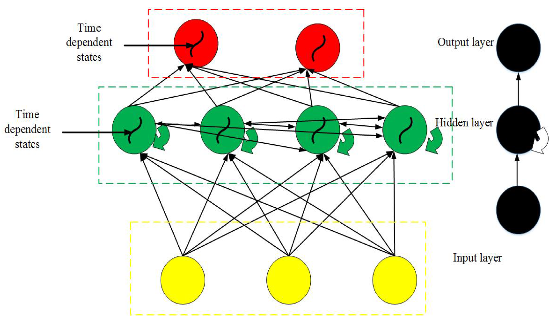
3.4. Recurrent Neural Network (RNN) Theory and Application in PPIR

Recurrent neural network (RNN) is another deep learning model that is mainly used for processing sequence data. In this model, the network has a memory function to store the data information from the previous time steps, i.e., there are both feedback and feedforward connections. The output from the previous time step is used as input to the next time step; therefore, it is also called a cyclic neural network. The neurons in the hidden layer of RNN are connected with one another, and the input of a neuron is composed of the data from the input layer and output of the neuron from the previous time step. The RNN can be mathematically expressed, as follows [32]:

$$z_h^l={\Sigma }_{i=1}^I{w}_{ih}{x}_i^t+{\Sigma }_{l^{\ast }}^L{w}_{l^{\ast }l}{a}_{l^{\ast }}^{t-1}$$

(8)

$$a_l^t=f_l\left(z_l^t\right)$$

(9)

$$y_k^t={\Sigma }_{l=1}^L{w}_{lk}{a}_h^t$$

(10)

In Equations (8)–(10), $x_i^t$ and $a_{l^{\ast }}^{t-1}$ represent the $ith$ and the $lth$ neurons in the input and hidden layers at time t, respectively. The value of the $lth$ neuron prior to the time instant t is given by $Z_h^l$, $y_k^t$ represents the $kth$ neuron in the output layer at time t, $w_{ih}$ represents the weight connecting the input and hidden layers, $w_{l^{\ast }l}$ represents the weight between the hidden layers, $w_{lk}$ represents the weight between the hidden and output layers, and $f_l\left(\right)$ represents the nonlinear activation function. The RNN has good dynamic characteristics and it can be generally divided into Jordan-type and Elman-type networks, where the former type belongs to the category of forward neural network with a local memory unit and local feedback connection. Figure 9 shows a typical RNN structure:

Figure 9. Typical Recurrent neural network (RNN) structure.

Initial applications of the RNN mainly included speech and handwriting recognition. However, in practice, the training of RNN is inefficient and it can take a considerable amount of time. Consequently, several researchers worked on improving the RNN structure [60]. In 2017, Mou et al. [61] put forward a new RNN model, which used a new activation function and parameter calibration. This model can effectively analyze hyperspectral pixels as sequence data and it could also adaptively produce a bounded output, and it had improved structural sparsity.

The RNN model has been recently applied to plant phenotypic images and it has considerable application prospects in the detection of complex disease plant phenotypes. In 2018, Lee et al. [58] combined the CNN and RNN for plant classification in order to deal with the problem of changes in the phenotypic appearance of plants. This model relied on capturing the dependencies between image pixels through the RNN model, and it could recognize the structural information in multiple plant images. The authors used the GRU (gated recurrent unit) in the RNN model, because GRU reduces the parameters by controlling the gate mechanism in order to alleviate the problem of gradient explosion or disappearance. The use of RNN enabled the learning of relationship between different features over a long time and reduced the number of parameters. Ndikumana et al. [59] aimed at the difficulties that were encountered in the development and improvement of agricultural coverage maps, and proposed an agricultural remote sensing image recognition method that is based on the RNN. The authors made use of the phase information present in the SAR (synthetic aperture radar) data. While using Sentinel-1 data, the authors classified different areas according to the plant phenotype, retaining the time based image structural information. The results showed that the RNN could extract the changes in plant phenotypic characteristics occurring over time and outperform traditional machine learning methods, such as KNN, SVM, RF (random forest), etc. The general steps in the work involved image preprocessing, normalization, and collection of images of different plants in order to establish an image library of plant specimens. The collected data set were used to train the RNN, while using its context memory learning ability and the image library in order to obtain the optimal training parameters, finally obtaining a complete classifier.

3.5. Stacked Autoencoder (SAE) Theory and Application in PPIR

The stacked autoencoder is a special deep learning model that has been widely used in data classification, image recognition, spectral processing, and anomaly detection. It consists of multiple automatic encoders that are stacked in series. By reducing the dimensions of the input data layer-by-layer, the higher-order features of the data are extracted and then input to the classification layer for classification [62,63]. The specific process of the SAE method is described, as follows: (1) given the initial input, the first-layer autoencoder is trained in an unsupervised manner in order to reduce the reconstruction error to the set value. (2) Take the output of the hidden layer of the first autoencoder as the input of the second autoencoder, and use the same method to train the autoencoder. (3) Repeat the second step until all of the auto encoders are initialized. (4) Use the output of the hidden layer of the last stacked autoencoder as the input of the classifier, and then use a supervised method to train the parameters of the classifier. In practical applications, a supervised learning network model requires a large number of labeled data samples to optimize network parameters, which is computationally intensive and not conducive to network training and learning. The earliest concept of the traditional auto-encoder was proposed by Rumelhart et al. [64], and its theoretical structure was analyzed, in detail, by Bourlard et al. [65].

In the field of PPIR, Liu et al. [66], in view of the complexity and uncertainty of traditional plant phenotypic characteristics extraction methods, put forward the mixed deep learning method. The authors combined the SAE and CNN models in order to classify plant leaves. Thanks to the automatic feature extraction ability, the experimental results showed that the combined models achieved significantly better results when compared to individual SAE, CNN, and SVM models. Cheng et al. [67] proposed a model for the image segmentation of flowers. The authors converted the RGB images to greyscale images, and used the SAE for the segmentation of osmanthus flowers under complex backgrounds. The proposed model used a three-layer structure for training of features extraction, followed by a final $Softmax$ layer for classification. The experimental results showed that this method could effectively reduce the image background noise in order to obtain effective plant phenotypic image classification and recognition. Wang et al. [68] showed that the classification accuracy of traditional machine learning methods for plant phenotype identification was low. The authors proposed a $k-$ sparse denoising encoder network classification for the recognition of plant leaves, effectively solving the over fitting problem. The authors showed the classification results with 44 types of plant leaves, reaching an accuracy of more than 95% for each type.

Figure 10 shows a diagram of Stacked autoencoder. The input X is first mapped to Y by a mapping function f, and Y is then converted back to X via a reconstruction function g. The goal during training is to reconstruct X, such that it is close to the input X. This is carried out by modifying a set of weights and encoding the input data. This process is carried out over multiple iterations, resulting in the minimization of the following loss function [69,70]:

$$H\left(W\right)={\displaystyle \underset{w.u}{\overset{argmin}{}}}{[\parallel X-U\mathsf{\Phi }\left(WX\right)\parallel }_2^2+\lambda R\left(W\right)]$$

(11)

Figure 10. Schematic diagram of Stacked Autoencoder (SAE) structure.

In Equation (11), X is the input data, W and U are the encoding and decoding weights, respectively, $\mathsf{\Phi }$ is the nonlinear activation function, $R\left(W\right)$ is defined according to the requirements, and $\lambda$ represents its weight. The SAE adopts deep feedforward neural network architecture, and the adjacent layer learning strategy is implemented by constructing the network in the form of a stack. In the image classification and recognition problem, the SAE is usually composed of two modules: feature learning and classifier. The general mathematical expression of a feature learning model is shown, as follows [69,70]:

$$X_l=S_l(W_{lg}{X}_{l-1}+b_l)\in R^{n_l},X_0=x$$

(12)

In the above expression, the feature learning stage has L hidden layers, where the number of nodes in each hidden layer is $n_l(l=1,2,3,\dots ,l)$, and the activation function is ${\delta }_l\left(\right)$. If the classifier model is based on the $Softmax$ function with k number of classes, and ${\theta }_k$ represents the learning parameters, then the model can be represented as [69,70]:

$$y\left(k\right)=\frac{e^{(X_L.{\theta }_k)}}{{\Sigma }_{j=1}^k{e}^{(X_L.{\theta }_j)}},y={[y\left(1\right),y\left(2\right),\dots ,y\left(k\right)]}^T$$

(13)

Figure 11 shows a flow chart of PPIR based on the SAE. First, the automatic encoders are stacked in order to build the neural network of deep learning, namely the coding area. Second, the input images are preprocessed that involves segmentation of greyscale images. Third, the preprocessed data are used to train stacked encoders based on a deep learning neural network. The features that are generated by the encoders are then used in order to generate classification results [69,70].

Figure 11. Stacked autoencoder identification flow chart.

Table 3 provides a summary of the aforementioned deep learning methods. Among them, the common experimental software for the four models include Pycharm, Matlab, OpenCV, etc. The original data forms include RGB vision, stereo vision, multispectral and hyperspectral, thermal imager, fluorescence, tomography, plant feature information matrix, etc.

Table 3. Deep learning network summary.

Model	Main task	References	Advantages	Disadvantages
CNN	Plant image classification, plant feature extraction, etc.	Gong et al., Grinblat et al., Dyrmann et al., Song et al. [39,40,41,42]	1. The training parameters are reduced, and the model has better generalization ability. 2. Pooling reduces the spatial dimensions of the network and requires less translation invariance of the input data.	1. Vanishing gradient problem can occur, poor identification of spatial features. 2. The accuracy of plant recognition decreases in the presence of high degree of image rotation.
DBN	Plant remote sensing image recognition, plant disease detection, plant feature information fusion, etc.	Liu et al., Deng et al., Yu et al., Guo et al. [53,54,55,56]	Ability to reflect the similarity of the same type data itself.	1. The accuracy is not high in classification problems. 2. Requires complex learning, input data should have translation invariance.
RNN	Multi-modal recognition of plant organs, plant disease detection, etc.	Sue et al., Ndikumana et al. [58,59]	Sequential plant feature information can be modeled.	There are many parameters to be trained, which can lead to vanishing or exploding gradient problem.
SAE	Plant image classification, plant image segmentation, etc.	Liu et al., Cheng et al., Wang et al. [66,67,68]	The encoded data are robust to noise, the training time is short, can learn the distribution subspace within a class, unsupervised extraction of features can save manpower and material resources.	1. Although training does not require labeled data, the performance is limited compared to supervised learning methods. 2. Greedy training mode is adopted, which can only achieve a local optimum. 3. Vanishing gradient problem can occur, there are many hyper parameters in the model, which require a long training time.

4. Common Problems and Future Outlook of Deep Learning in PPIR

(1) There are several factors to consider in applications of deep learning, such as the number of layers, architecture, learning algorithm used in the neural network to optimize weights, and biases, etc. [71]. In addition, in the process of PPIR, deep learning relies heavily on big data, while the big data of plant phenotypic rely heavily on expert knowledge, the optimization model needs to be adjusted by trial and error according to different kinds of plants. In the future, the development and testing of different models to maximize the extraction of the feature information and achieve optimal model precision is an important research direction. Furthermore, emerging deep learning models, such as generative adversarial network (GAN) and capsule network (CapsNet), can have broad application prospects for PPIR [72]. Researchers prefer supervised models in deep learning, mainly because the characteristics of many plant phenotypes are difficult to understand and obtain, and the learning of unsupervised models tends to lead to disorder.

(2) In deep learning networks, another important factor is the training speed. Generally speaking, a higher number of training iterations improves the accuracy at the expense of a longer training time, which will affect the simulation results. Therefore, the relationships between the network scale, accuracy requirements, and training speed should be comprehensively adjusted during the whole application process. In addition, the experiments show that the selection of an appropriate classifier for different plant phenotypic characteristics information can improve the classification performance of deep learning networks [73,74].

(3) Changes in input data during the plant phenotypic image acquisition, such as image size, pixel, translation, scaling, occlusion, and other uncertainties, affect the output results [75,76]. Plant phenotype recognition from complex background images directly affects the classification results. In other words, the PPIR lacks unified standards and, consequently, it is difficult to achieve a quantitative comparison between deep learning models that are applied to different types of plant species [7]. In addition, as the collection of image data is influenced by regional restrictions, plant varieties, and the types of diseases, individual researchers construct the data sets based on their individual rules. Therefore, building a general plant phenotypic database that can be used as a benchmark is essential.

(4) Several researchers work on extracting new plant features. However, there are several open questions in this context: (a) are the plant features easy to extract? (b) Are they significantly affected by noise? (c) Can they be used to accurately distinguish different kinds of plants? In fact, the application of plant phenotypes is mainly aimed at genetic omics, which is the changes in crop characteristics that correspond to the genetic changes. In recent years, it has been applied to crop shape control, breeding, species identification, irrigation control, and disease early warning. Generally speaking, with the changing time and environment, the color or shape of the same plant may also change; therefore, the selection of appropriate features for use in PPIR is an important issue that is to be considered in future studies [77,78].

5. Conclusions

First, this paper introduces, compares, and analyzes traditional methods of plant phenotypic image recognition. Second, it explains the theory of four types of deep learning network models and their applications in PPIR. Finally, it discusses their existing applications and future development directions. When compared to the traditional PPIR algorithms, the deep learning models perform better, as they can explore detailed and higher number of image characteristics and have a high recognition accuracy. The convolutional neural networks are one of the most widely used deep learning models in PPIR with the most effective performance. PPIR technology has broad application prospects and research value in the future era of smart agriculture and big data development. Deep learning network theory, architecture for identification of 3D plant models, and the establishment of online plant recognition systems are a future direction of development in the field of plant phenotypic image recognition.

References

- Wang, Z.B.; Li, H.L.; Zhu, Y.; Xu, T.F. Review of plant identification based on image processing. Arch. Comput. Methods Eng. 2017, 24, 637–654. [Google Scholar] [CrossRef]
- Mohanty, S.P.; Hughes, D.P.; Salathé, M.L. Using deep learning for image-based plant disease detection. Front. Plant Sci. 2016, 7, 14–19. [Google Scholar] [CrossRef] [PubMed]
- Zhang, N.; Liu, W.P. Plant leaf recognition technology based on image analysis. Appl. Res. Comput. 2011, 18, 7–13. [Google Scholar]
- Javed, A.; Nour, M.; Hasnat, K.; Essam, D.; Waqas, H.; Abdul, W. A review of intrusion detection systems using machine and deep learning in internet of things: Challenges, solutions and future directions. Electronics 2020, 9, 1177. [Google Scholar]
- Ma, Z.Y. Research and Test on Plant Leaves Recognition System Based on Deep Learning and Support Vector Machnie; Inner Mongolia Agricultural University: Hohhot, China, 2016. [Google Scholar]
- Muhammad, A.F.A.; Lee, S.C.; Fakhrul, R.R.; Farah, I.A.; Sharifah, R.W.A. Review on techniques for plant leaf classification and recognition. Computers 2019, 8, 77. [Google Scholar]
- Weng, Y.; Zeng, R.; Wu, C.M.; Wang, M.; Wang, X.J.; Liu, Y.J. A survey on deep-learning-based plant phenotype research in agriculture. Sci. Sin. 2019, 49, 698–716. [Google Scholar] [CrossRef]
- Barbedo, J.G.A. A review on the main challenges in automatic plant disease identification based on visible range images. Biosyst. Eng. 2016, 144, 52–60. [Google Scholar] [CrossRef]
- Cope, J.S.; Corney, D.; Clark, J.Y.; Remagnino, P.; Wilkin, P. Plant species identification using digital morphometrics: A review. Expert Syst. Appl. 2012, 39, 7562–7573. [Google Scholar] [CrossRef]
- Waldchen, J.; Mader, P. Plant Species Identification Using Computer Vision Techniques: A Systematic Literature Review. Arch. Comput. Methods Eng. 2016, 25, 507–543. [Google Scholar] [CrossRef]
- Thyagharajan, K.K.; Raji, I.K. A Review of Visual Descriptors and Classification Techniques Used in Leaf Species Identification. Arch. Comput. Methods Eng. 2019, 26, 933–960. [Google Scholar] [CrossRef]
- Ingrouille, M.J.; Laird, S.M. A quantitative approach to oak variability in some north London woodlands. Comput. Appl. Res. 1986, 65, 25–46. [Google Scholar]
- Yonekawa, S.; Sakai, N.; Kitani, O. Identification of idealied leaf types using simple dimensionless shape factors by image analysis. Trans. ASAE 1993, 39, 1525–1533. [Google Scholar] [CrossRef]
- Cheng, S.C.; Jhao, J.J.; Liou, B.H. PHD plant search system based on the characteristics of leaves using fuzzy function. New Trends Artif. Intell. 2007, 5, 834–844. [Google Scholar]
- Villena, R.J.; Lana, S.S.; Cristobal, J.C.G. Daedalus at image CLEF 2011 plant identification task: Using SIFT keypoints for object detection. In Proceedings of the CLEF 2011 Labs and Workshop, Amsterdam, The Netherlands, 19–22 September 2011. [Google Scholar]
- Charles, M.; James, C.; James, O. Plant leaf classification using probabilistic integration of shape, texture and margin features. Comput. Graph. Imaging 2013, 5, 45–54. [Google Scholar] [CrossRef]
- Wang, X.F.; Huang, D.S.; Du, J.X.; Zhang, G.J. Feature extraction and recognition for leaf images. Comput. Eng. Appl. 2006, 3, 190–193. [Google Scholar]
- Wang, N.; Wang, K.R.; Xie, R.Z.; Lai, J.C.; Ming, B.; Li, S.K. Maize leaf disease identification based on fisher discrimination analysis. Sci. Agric. Sin. 2009, 42, 3836–3842. [Google Scholar]
- Zhai, C.M.; Du, J.X. A plant leaf image matching method based on shape context features. J. Guangxi Norm. Univ. (Nat. Sci. Ed.) 2009, 27, 171–174. [Google Scholar]
- Wang, L.J.; Huai, Y.J.; Peng, Y.C. Method of identification of foliage from plants based on extraction of multiple features of leaf images. J. Beijing For. Univ. 2015, 37, 55–61. [Google Scholar]
- Cen, H.Y.; Lu, R.F.; Zhu, Q.B.; Fernando, M. Nondestructive detection of chilling injury in cucumber fruit using hyperspectral imaging with feature selection and supervised classification. Postharvest Biol. Technol. 2016, 111, 352–361. [Google Scholar] [CrossRef]
- Zhang, S. Research on Plant Leaf Images Identification Algorithm Based on Deep Learning; Beijing Forestry University: Beijing, China, 2016. [Google Scholar]
- Osikar, J.O. Computer Vision Classification of Leaves from Swedish Trees; Linkoing University: Linköping, Sweden, 2001. [Google Scholar]
- Iqbal, Z.; Khan, M.A.; Sharif, M.; Shah, J.H.; Rehman, M.H.; Javed, K. An automated detection and classification of citrus plant diseases using image processing techniques: A review. Comput. Electron. Agric. 2018, 152, 12–32. [Google Scholar] [CrossRef]
- Zhao, Q.Y.; Kong, P.; Min, J.Z. A review of deep learning methods for the detection and classification of pulmonary nodules. J. Biomed. Eng. 2019, 36, 1060–1068. [Google Scholar]
- Huo, Y.Q.; Zhang, C.; Li, Y.H.; Zhi, W.T.; Zhang, J. Nondestructive detection for kiwifruit based on the hyperspectral technology and machine learning. J. Chin. Agric. Mech. 2019, 40, 71–77. [Google Scholar]
- Liu, Y.; Chen, X.; Wang, Z.F.; Ward, R.K.; Wang, X.S. Deep learning for pixel-level image fusion: Recent advances and future prospects. Inf. Fusion 2018, 42, 158–173. [Google Scholar] [CrossRef]
- Sladojevic, S.; Arsenovic, M.; Anderla, A.; Culibrk, D. Deep neural networks based recognition of plant diseases by leaf image classification. Comput. Intell. Neurosci. 2016, 2016. [Google Scholar] [CrossRef] [PubMed]
- Singh, A.; Ganapathysubramanian, B.; Singh, A.K.; Sarkar, S. Machine learning for high-throughput stress phenotyping in plants. Trends Plant Sci. 2016, 21, 110–124. [Google Scholar] [CrossRef] [PubMed]
- Liu, H.; Coquin, D.; Valet, L.; Cerutti, G. Leaf species classification based on a botanical shape sub-classifier strategy. In Proceedings of the 2014 22nd International Conference on Pattern Recognition, Stockholm, Sweden, 24–28 August 2014; pp. 24–28. [Google Scholar]
- Hinton, G.E.; Salakhutdinov, R.R. Reducing the dimensionality of data with neural networks. Science 2006, 313, 504–507. [Google Scholar] [CrossRef]
- Zhao, C.J.; Lu, S.L.; Guo, X.Y.; Du, J.J.; Wen, W.L.; Miao, T. Advances in research of digital plant: 3D Digitization of Plant Morphological Structure. Sci. Agric. Sin. 2015, 48, 3415–3428. [Google Scholar]
- Yu, K.; Jia, L.; Chen, Y.Q.; Xu, W. Salakhutdinov, R.R. Deep learning: Yesterday, today, and tomorrow. J. Comput. Res. Dev. 2013, 50, 1799–1804. [Google Scholar]
- Garcia, G.A.; Escolano, O.S.; Oprea, S.; Martinez, V.V.; Gonzalez, P.M.; Rodriguez, J.G. A survey on deep learning techniques for image and video semantic segmentation. Appl. Soft Comput. 2018, 70, 41–65. [Google Scholar] [CrossRef]
- Lecun, Y.; Bottou, L.; Bengio, Y.; Haffner, P. Gradient-based learning applied to document recognition. Proc. IEEE 1998, 86, 2278–2324. [Google Scholar] [CrossRef]
- Zeiler, M.D.; Krishnan, D.; Taylor, G.W.; Fergus, R. Deconvolutional networks. In Proceedings of the 2010 IEEE Conference on Computer Vision And Pattern Recognition (CVPR), San Francisco, CA, USA, 13–18 June 2010; pp. 2528–2535. [Google Scholar]
- Yu, F.W.; Chen, J.L.; Duan, L.X. Exploiting images for video recognition: Heterogeneous feature augmentation via symmetric adversarial learning. IEEE Trans. Image Process. 2019, 28, 5308–5321. [Google Scholar] [CrossRef]
- Gyires, T.B.P.; Osváth, M.; Papp, D.; Szűcs, G. Deep learning for plant classification and content-based image retrieval. Cybern. Inf. Technol. 2019, 19, 88–100. [Google Scholar]
- Dyrmann, M.; Karstoft, H.; Midtiby, H.S. Plant species classification using deep convolutional neural network. Biosyst. Eng. 2016, 151, 72–80. [Google Scholar] [CrossRef]
- Gong, D.X.; Cao, C.R. Plant leaf classification based on CNN. Comput. Mod. 2014, 4, 12–19. [Google Scholar]
- Grinblat, G.L.; Uzal, L.C.; Larese, M.G.; Granitto, P.M. Deep learning for plant identification using vein morphological patterns. Comput. Electron. Agric. 2016, 127, 418–424. [Google Scholar] [CrossRef]
- Song, X.Y.; Jin, L.T.; Zhao, Y.; Sun, Y.; Liu, T. Plant image recognition with complex background based on effective region screening. Laser Optoelectron. Prog. 2019, 57, 10–16. [Google Scholar]
- Pan, J.Z.; He, Y. Recognition of plants by leaves digital image and neural network. In Proceedings of the 2008 International Conference on Computer Science and Software Engineering, Wuhan, China, 12–14 December 2008; pp. 906–910. [Google Scholar]
- Zhou, F.Y.; Jin, L.P.; Dong, J. Review of convolutional neural networks. Chin. J. Comput. 2017, 40, 1229–1251. [Google Scholar]
- Ferentinos, K.P. Deep learning models for plant disease detection and diagnosis. Comput. Electron. Agric. 2018, 145, 311–318. [Google Scholar] [CrossRef]
- Hang, J.; Zhang, D.X.; Chen, P.; Zhang, J.; Wang, B. Classification of plant leaf diseases based on improved convolutional neural network. Sensors 2019, 19, 4161. [Google Scholar] [CrossRef]
- Liu, T.T.; Wang, T.; Hu, L. Rhizocotonia solani recognition algorithm based on convolutional neural network. Chin. J. Rice Sci. 2019, 33, 90–94. [Google Scholar]
- Zhang, J.; Huang, X.Y. Species identification of prunus mume based on image analysis. J. Beijing For. Univ. 2012, 34, 96–104. [Google Scholar]
- Zhang, H.T.; Mao, H.P.; Qiu, D.Y. Feature extraction for the stored-grain insect detection system based on image recognition technolog. Trans. Chin. Soc. Agric. Eng. 2009, 25, 126–130. [Google Scholar]
- Jiang, M.Y.; Liang, Y.C.; Feng, X.Y.; Fan, X.J.; Pei, Z.L.; Xue, Y.; Guan, R.C. Text classification based on deep belief network and softmax regression. Neural Comput. Appl. 2018, 29, 61–70. [Google Scholar] [CrossRef]
- Fatahi, M.; Shahsavari, M.; Ahmadi, M.; Ahmadi, A.; Boulet, P.; Devienne, P. Rate-coded DBN: An online strategy for spike-based deep belief networks. Biol. Inspired Cogn. Archit. 2018, 24, 59–69. [Google Scholar] [CrossRef]
- Li, T.; Sun, J.G.; Zhang, X.J.; Wang, X. Spectral-spatial joint classification method of hyperspectral remote sening image. Chin. J. Sci. Instrum. 2016, 37, 1379–1389. [Google Scholar]
- Liu, N.; Kan, J.M. Plant leaf identification based on the multi-feature fusion and deep belief networks method. J. Beijing For. Univ. 2016, 38, 110–119. [Google Scholar]
- Deng, X.W.; Qi, L.; Ma, X.; Jiang, Y.; Chen, X.S.; Liu, H.Y.; Chen, W.F. Recognition of weeds at seedling stage in paddy fields using multi-feature fusion and deep belief neworks. Trans. Chin. Soc. Agric. Eng. 2018, 34, 165–172. [Google Scholar]
- Yu, Y.H.; Li, H.G.; Shen, X.F.; Feng, Y. Study on multiple varieties of maize haploid qualitative identification based on deep belief network. Spectrosc. Spectr. Anal. 2019, 39, 905–909. [Google Scholar]
- Guo, D.; Lu, Y.; Li, J.N.; Jiang, F.; Li, A.C. Identification method of rice sheath blight based on deep belief network. J. Agric. Mech. Res. 2019, 41, 42–45. [Google Scholar]
- Liu, F.Y.; Wang, S.H.; Zhang, Y.D. Survey on deep belief network model and its applications. Comput. Eng. Appl. 2018, 54, 11–18. [Google Scholar]
- Lee, S.H.; Chan, C.S.; Remagnino, P. Multi-organ plant classification based on convolutional and recurrent neural networks. IEEE Trans. Image Process. 2018, 27, 4287–4301. [Google Scholar] [CrossRef] [PubMed]
- Ndikumana, E.; Minh, D.H.T.; Baghdadi, N.; Courault, D.; Hossard, L. Deep recurrent neural network for agricultural classification using multitemporal SAR sentinel-1 for camargue, France. Remote Sens. 2018, 10, 1217. [Google Scholar] [CrossRef]
- Jain, A.; Zamir, A.R.; Savarese, S.; Saxena, A. Structural-RNN: Deep learning on spatio-temporal graphs. In Proceedings of the 2016 IEEE Conference on Computer Vision and Pattern Recognition, Las Vegas, NV, USA, 27–30 June 2016; pp. 5308–5317. [Google Scholar]
- Mou, L.C.; Ghamisi, P.; Zhu, X.X. Deep recurrent neural networks for hyperspectral image classification. IEEE Trans. Geosci. Remote Sens. 2017, 55, 3639–3654. [Google Scholar] [CrossRef]
- Edoardo, R.; Erik, C.; Rodolfo, Z.; Paolo, G. A Survey on deep learning in image polarity detection: Balancing generalization performances and computational costs. Electronics 2019, 8, 783. [Google Scholar]
- Malek, S.; Melgani, F.; Bazi, Y.; Alajlan, N. Reconstructing cloud-contaminated multispectral images with contextualized autoencoder neural networks. IEEE Trans. Geosci. Remote Sens. 2018, 56, 2270–2282. [Google Scholar] [CrossRef]
- Rumelhart, D.E.; Hinton, G.E.; Bazi, Y.; Williams, R.J. Learning representations by back-propagating errors. Nature 1986, 323, 533–536. [Google Scholar] [CrossRef]
- Bourlard, H.; Kamp, Y. Auto-asscoiation by multilayer perceptrons and singular value decomposition. Biol. Cybemetics 1988, 59, 291–294. [Google Scholar] [CrossRef]
- Liu, Z.; Zhu, L.; Zhang, X.P.; Zhou, X.B.; Shang, L.; Huang, Z.K.; Can, Y. Hybrid deep learning for plant leaves classification. In Proceedings of the International Conference on Intelligent Computing, Fuzhou, China, 20–23 August 2015; pp. 115–123. [Google Scholar]
- Cheng, Y.Z.; Duan, Y.F. O.fragrans luteus image segmentation method based on stacked autoencoder. J. Chin. Agric. Mech. 2018, 39, 77–80. [Google Scholar]
- Wang, X. Research on Plant Leaf Image Classification Based on Stacked Auto-Encoder Network; Nanchang University: Nanchang, China, 2019. [Google Scholar]
- Yuan, F.N.; Zhang, L.; Shi, J.T.; Xia, X.; Li, G. Theories and applications of auto-encoder neural networks: A literature survey. Chin. J. Comput. 2019, 42, 203–230. [Google Scholar]
- Siti, N.; Annisa, D.; Akhmad, N.S.M.; Muhammad, N.R.; Firdaus, F.; Bambang, T. Deep learning-based stacked Denoising and autoencoder for ECG heartbeat classification. Electronics 2020, 9, 135. [Google Scholar]
- Lei, S.; Kenneth, M.; Gordon, R.O. Hyperspectral image classification with stacking spectral patches and convolutional neural networks. IEEE Trans. Geosci. Remote Sens. 2018, 56, 5975–5984. [Google Scholar]
- Dinh, H.T.M.; Ienco, D.; Gaetano, R.; Lalande, N.; Ndikumana, E.; Osman, F.; Maurel, P. Deep recurrent neural networks for winter vegetation quality mapping via multitemporal SAR sentinel-1. IEEE Geosci. Remote Sens. Lett. 2018, 15, 464–468. [Google Scholar]
- Lee, S.H.; Chan, C.S.; Mayo, S.J.; Remagnino, P. How deep learning extracts and learns leaf features for plant classification. Pattern Recognit. 2017, 71, 1–13. [Google Scholar] [CrossRef]
- Nagasubramanian, K.; Jones, S.; Singh, A.K.; Sarkar, S.; Singh, A.; Ganapathysubramanain, B. Explaining hyperspectral imagiing based plant disease identification: 3D CNN and saliency maps. Plant Methods 2019, 15, 1–10. [Google Scholar] [CrossRef]
- Alwaseela, A.; Cen, H.Y.; Ahmed, E.; He, Y. Infield oilseed rape images segmentation via improved unsupervised learning models combined with supreme color features. Comput. Electron. Agric. 2019, 162, 1057–1068. [Google Scholar]
- Raghu, P.P.; Yegnanarayana, B. Supervised texture classification using a probabilistic neural network and constraint satisfaction model. IEEE Trans. Neural Netw. 1998, 9, 516–522. [Google Scholar] [CrossRef]
- Singh, K.; Gupta, I.; Gupta, S. SVM-BDT PNN and fourier moment technique for classification of leaf shape. Int. J. Signal Process Image Process Pattern Recognit. 2010, 3, 67–78. [Google Scholar]
- Zhao, C.J. Big data of plant phenomics and its research progress. J. Agric. Big Data 2019, 1, 5–18. [Google Scholar]
Publisher’s Note: MDPI stays neutral with regard to jurisdictional claims in published maps and institutional affiliations. |
© 2021 by the authors. Licensee MDPI, Basel, Switzerland. This article is an open access article distributed under the terms and conditions of the Creative Commons Attribution (CC BY) license (http://creativecommons.org/licenses/by/4.0/).