Abstract
Recovery of three-dimensional (3D) coordinates using a set of images with texture mapping to generate a 3D mesh has been of great interest in computer graphics and 3D imaging applications. This work aims to propose an approach to adaptive view selection (AVS) that determines the optimal number of images to generate the synthesis result using the 3D mesh and textures in terms of computational complexity and image quality (peak signal-to-noise ratio (PSNR)). All 25 images were acquired by a set of cameras in a array structure, and rectification had already been performed. To generate the mesh, depth map extraction was carried out by calculating the disparity between the matched feature points. Synthesis was performed by fully exploiting the content included in the images followed by texture mapping. Both the 2D colored images and grey-scale depth images were synthesized based on the geometric relationship between the images, and to this end, three-dimensional synthesis was performed with a smaller number of images, which was less than 25. This work determines the optimal number of images that sufficiently provides a reliable 3D extended view by generating a mesh and image textures. The optimal number of images contributes to an efficient system for 3D view generation that reduces the computational complexity while preserving the quality of the result in terms of the PSNR. To substantiate the proposed approach, experimental results are provided.
Keywords:
array cameras; light field camera; adaptive view selection; view synthesis; mesh; texture; depth map 1. Introduction
The tree-dimensional (3D) coordinates of a real-world scene provide rich information for 3D geometric and photometric reconstruction. Reconstruction work has been considered one of the major goals in the area of computer vision. Furthermore, view synthesis has also been of great interest in diverse applications such as computer graphics, 3D imaging, 3D rendering, and virtual/augmented reality [1,2,3,4,5,6]. Thanks to the significant improvement of the hardware of computers, one can achieve fast and accurate results for 3D rendering, view synthesis, and 3D reconstruction [7,8]. In reconstruction work, two main approaches have been widely used: one is called the passive method, and the other one is called the active method. Although these two methods are considered traditional ones, they still provide accurate and stable reconstruction results in practice [9,10,11,12]. The passive method uses multiple cameras (usually two) that are located at different positions, and the active method uses a camera(s) and a light source(s). Both the passive and active methods basically obey the principle of triangulation defined by the locations of the camera(s), the light source(s), and a point of the 3D object. In the passive method, all of the cameras, having different perspectives, capture the same target object, and any point of the target in the 3D space is projected onto the 2D image planes, each of which belongs to each of the camera. The different positions of the cameras generate relative rotations and translations among the images. Stereo vision, which uses two cameras, has the advantages of a simple experimental setup and a concise algorithm and mathematical modeling. In general, to calculate the 3D coordinates of a target object, the stereo vision algorithm is expected to achieve highly accurate feature extraction and successful correspondence matching, leading to a high accuracy of disparity and depth estimation. Camera calibration is a task to estimate the internal and external parameters of cameras, and it is one of the most crucial for accurate 3D measurement. The internal parameters consist of the focal length, skewness factor, and the principal points of an image. The external parameters consist of the relative rotation and translation of the optical centers. Since Tsai’s approach in the 1980s, calibration algorithms have been proposed for more accurate estimation of the internal and external parameters, and almost for the past two decades, Zhang’s algorithm has been the most widely used in the research and industrial fields [13,14]. In 2000, a circular pattern for the calibration was also proposed, and the work reported that the results of the internal and external parameters showed a smaller standard deviation [15]. Calibration requires high computational complexity because the estimation of the parameters is from the iteration of the procedures of the calibration and optimization. Overfitting of the optimization or inaccurate feature extraction/matching may cause a large error in the calibration result. The passive method suffers from a low-light condition, a texture-less object, or a repetitively patterned scene [16,17]. Recently, the passive method employed the deep neural network model to improve the accuracy and quality of depth estimation, but this approach did not resolve the fundamental limitations inherent to the passive method [18].
The active method can alleviate the limitations of the passive method by using the properties of structured light patterns or light rays. The active method uses both a camera and a light source, which emits light patterns or rays onto a target object [19]. In the structured light pattern approaches, specific patterns, the structures of which are already known, are projected onto a 3D target object, and the shape of the object’s surface deforms the patterns. In the light ray based approaches, the light source emits light rays onto a target object, and the distance between the viewpoint and a point of the target is calculated based on the measurement of the round-trip time of the emitted light ray signal. The active method using a time-of-flight (TOF) sensor is one of the main technologies to facilitate the 3D reconstruction. Recently, the TOF employed the deep neural network model to directly recover the depth information of a 3D scene to alleviate the limitations of the conventional TOF, which accumulates errors occurring during all of the procedures for depth recovery such as light emission, sensor calibration, resolving light interference, denoising, etc. The deep neural network model learns various scenes and provides an end-to-end framework for direct depth calculation. Since the TOF uses only a single light ray, which travels at a very high speed, it has a limitation in its depth resolution [20]. The structured light pattern based approach improves the depth resolution by using a light pattern, the density of which can be flexibly adjusted. Furthermore, information about structure of the pattern can provide sufficient information to recover 3D coordinates of a target object. While the TOF does not require the principle of triangulation, the structured light approach utilizes triangulation just as the passive method does. To achieve a high accuracy in the reconstruction result, correspondence matching between the projected light patterns and the reflected light patterns needs to be performed with high confidence. In the early stage of the structured light pattern approach, simple patterns such as dots or vertical, horizontal, or gridded lines were used [21,22]. However, this method sometimes suffers from an inaccurate correspondence matching between the original and the deformed patterns because the patterns are repetitive ones. Colored patterns, or the patterns with various coding schemes, or the patterns emitted with a varying phase (e.g., sinusoidal patterns) could alleviate the limitations of the correspondence matching [23,24]. Recently, in the active method, the deep neural network model was employed for pattern classification and identification, which successfully achieved the accurate correspondence matching of the patterns with blurring, a low resolution, or geometric distortions [25]. In the past few decades, significant improvement in the reconstruction has been observed using the passive or the active method, and recently, the approaches based on fusing the passive and the active methods (also called hybrid methods) have contributed to the improvement of the reconstruction accuracy by alleviating the limitations inherent to each method, as explained above [26,27].
Different from the conventional methods, e.g., the passive or the active ones, light field camera technology provides 3D reconstruction, rendering, view synthesis, and refocus results that enable one to generate real-world 3D scenes with high fidelity [28,29,30]. In the early work on light field cameras (also called plenoptic cameras), a set of lenses or cameras performs the scene reconstruction based on the direction of the light rays, the wavelength, the locations of the 3D points, etc., modeled as a plenoptic function (Equation (1)), which has been successfully applied to various practical fields such as rendering, view synthesis, 3D reconstruction, etc. [31,32]. The work of Levoy in 1996 is considered as a cornerstone of the research on light field cameras for 3D reconstruction [31,33]. The work proposed a novel approach to interpolating views to generate a novel viewpoint using the information of the light field, but the approach does not rely on depth information and accurate feature matching. Multiple images of the array structure (called array images) and the light rays coming from each of them construct the new views; to this end, the 3D rendering of a real-world scene is performed with efficiency and accuracy. Since a single point on the surface emits multiple rays with different directions and intensities, the light field camera enables us to reconstruct or generate novel views [34,35]. Previous work on light field cameras focused on accurate 3D reconstruction or depth measurements themselves. Thus, accurate depth estimation for 3D reconstruction is still the most important task. To achieve 3D representation with efficiency and accuracy, mesh generation and texture mapping have been of interest in computer graphics, rendering, virtual/augment reality, etc. As method similar to the conventional method of 3D reconstruction, the depth and color information basically provides sufficient information to generate the mesh, and a layered depth image enables us to design efficient (high speed) texture mapping.
By generating a polygonal mesh using the Delaunay triangle rather than generating the pixel based depth, the reconstruction of a 3D object or scene can be restated as an approximation problem [36]. Although approximation can degrade the accuracy of the reconstruction result, it can accelerate the speed and can simplify the reconstruction algorithm. In the light field camera system, the performance of the result depends on the accuracy of the estimation of the parameters in the plenoptic functions that represent the light rays coming from the 3D space, which is written as follows:
where (, ) represents the direction of the light rays, is the wavelength, and () and t are the 3D coordinated of the real scene and the time, respectively. If p is known, that means we know all of the information about the light rays coming from the real-world scene.
In this paper, we present a method called adaptive view selection (AVS) to efficiently represent a synthesized three-dimensional model using a set of images and corresponding depth images that are basically used to generate the mesh and perform texture mapping. The present work is different from the previous work on view synthesis in that this work focuses on synthesizing the 3D models of a scene by synthesizing both the color images and the depth images.
In the light field camera, the accurate estimation of the parameters in the plenoptic function requires many images (dense sampling). This leads to computational inefficiency, and it may be impossible to embed it into mobile devices. Furthermore, the diffraction or interferenceof light can degrade the quality of the results of the reconstruction, rendering, or depth estimation. The quality of the light field imaging depends on both the number of images and the density of the light field, so the interpolating view is one of the most important tasks for the light field camera [37]. Interpolation is considered a simple and efficient method to increase the resolution of an image, so it is widely used in image processing. Akin to image processing, the interpolating view or the interpolating plenoptic function can generate a novel view and increase the angular resolution. However, the interpolation approach can degrade the image quality if the estimation of the existing view or the estimation of the change of the viewpoint is inaccurate [38].
Inspired by the success in the areas of imaging and computer vision, in the past few years, light field cameras have started utilizing the deep neural network (DNN) model [39]. The DNN model contributes to solving the problems of the trade-off between the spatial resolution and the angular resolution inherent to light field cameras. The typical steps for view synthesis or 3D reconstruction using light field cameras are composed of the depth estimation and the geometric/photometric image compensation, such as warping, rotation, and translation due to different perspectives. The DNN model learns and estimates two main aspects: one is depth, and the other one is image compensation. The results of light field camera applications inevitably depend on the depth of a scene, and existing work considered accurate depth estimation as one of the most crucial applications. To predict the depth value from light field images, the convolutional neural network (CNN) has been employed to provide an end-to-end framework for depth prediction. To achieve accurate results, a tremendous amount of data is generated by data augmentation. Although this work shows promising results in that the neural network model can be adequately applied to light field cameras, it is limited to depth prediction [40]. In practice, light field cameras have the issue of the quality degradation of the depth due to the non-uniform distribution of the light field. The learning based framework to find the best configuration that can provide the best depth estimation has been performed by augmenting and training the dataset and minimizing the matching cost based on the differences in the gradient and color information of the images. This work contributed to alleviating the depth distortion problem, but it still suffers from a texture-less target object [41]. The previous work, as mentioned above, chiefly dealt with depth estimation or accurate image warping to generate a novel view or 3D reconstruction results. In this paper, we chiefly deal with the adaptive selection of the images and the analysis of the computation time and the image quality of the synthesized results with 3D polygonal mesh generation and texture mapping. In addition to the synthesis of the colored and depth images using the array cameras, the proposed work presents the adaptive selection of the images, that is finding the optimal number of images that can provide a reliable synthesis result, but the number of images selected is less than the number of the elements of the array cameras (25 cameras in this paper). Akin to the Nyquist rate in signal processing, we focus on the determination of the sampling criterion for a reliable result. Image-wise sampling is employed in this work, and the whole sampling rate corresponds to 25, which is the size of the array. Fully exploiting 2D colored and grey-scaled depth images, the mesh generation and texture mapping are carried out using only the selected images. This work is different from IBR (image based rendering) in that our work employs geometric information, a depth map, and colored-image data [42]. The synthesis work is carried out using both the estimated depth and color information of the images. Once the depth map is generated for each image, matching between the depth map and color information is carried out so that the synthesis of the depth images can be successful. In particular, the quality of the representation is based on the technique of synthesizing images and depth information, and the results of the synthesis depend on the quality of the transition of the image content that overlaps among neighboring images. There have been numerous works on image synthesis that provided a successful transition between images that contain common contents, leading to overlapped regions, but these works did not perform synthesis using the depth map [43].
In the experiment in this paper, we propose an approach to view synthesis with mesh generation and texture mapping using a light field (plenoptic) camera composed of 25 cameras ( array). The present work is different from the previous work in that not only image synthesis, but also the synthesis of the depth map is performed to provide the synthesized 3D model of the target scene. This work is also different from the existing work in that this work also focuses on the depth map estimation, which takes into account occlusion based on the gradient, and the occlusion problem is resolved to provide a higher quality mesh. In the previous work, in general, the light field camera focused on the 3D reconstruction itself to provide a better result than conventional reconstruction methods, rather than other aspects such as image representation, synthesis, etc. In addition to the depth map and mesh generation, this paper proposes an approach to view and depth map synthesis that generates an extended view of a scene, which is difficult using only a single camera. This work hence provides an extended view and depth with a single capture using a set of cameras, i.e., array cameras. If a wide field-of-view (FOV) camera is given, it is easy to acquire the scene with the extended view, but this requires changing the hardware or the whole camera system, which incurs a high cost. By using array cameras, with the synthesis algorithm, the extended view can be provided without high cost custom hardware, and the configuration of each camera can generate various effects in the image results. This paper proceeds to generate the 3D mesh and perform texture mapping followed by depth map estimation. Depth images are generated corresponding to each image, which is an element of the array camera system. The depth map estimation is similar to that using a stereo camera system, but not only neighboring (or adjacent) images, but also any pair of images is used to generate the depth map. The selection of the images affects the depth map result. For example, a pair of images is selected from the top right and top left; the disparity may be larger than other selections, but the area of the overlapped regions will be the smallest. However, if adjacent images are selected, the area of the overlapped regions may be the largest. The former case is able to provide the largest extended view, but the latter one may provide the smallest extension. However, the latter case can provide an accurate stitching result because there are sufficient overlapped regions with feature points. Each viewpoint of the 25 cameras generates a corresponding depth map, and the depth map synthesis and RGB image synthesis are simultaneously carried out to provide an extended 3D view of a real-world scene. By increasing the number of cameras, the computational complexity increases accordingly, but in this paper, we propose an approach to view synthesis with the adaptive selection of the images. In other words, we demonstrate that less than 25 images can generate a 3D representation of a scene with the mesh and texture mapping while preserving the quality of the result using 25 images. In this paper, we describe how to find the optimal number of input images that can generate reliable results of mesh generation and texture mapping for a 3D view synthesis result by showing the computational complexity and image quality. In particular, to find the optimal number of images for the 3D synthesis, the sampling criterion is determined based on the contents of the input images. Feature matching between the images and the corresponding depth map provide the optimal coverage of a target scene that minimizes the overlapped regions. Overview of the present work is shown in Figure 1.
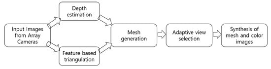
Figure 1.
Flow diagram of generating an extended 3D view using a set of images using array cameras.
The rest of the paper is organized as follows. Section 2 details the depth map generation using images from different viewpoints. Section 3 is about the view synthesis with adaptive view selection, which contributes to the efficient system with respect to the computational complexity. Section 4 presents 3D mesh generation followed by texture mapping. Section 5 substantiates the proposed AVS by showing the experimental results using the images captured by the array cameras before we conclude this paper.
2. Depth Map Generation for Synthesis
This section provides the details about generating the depth map for synthesizing grey-scaled depth images. The depth map is generated based on the parallax between neighboring images captured by array cameras. In the course of depth map generation, gradient based detection of occlusion is discussed. Any pair of images can generate a depth map, while occlusion is always taken into account, and disparities are calculated between matched feature points, for which the array cameras are already calibrated. In the existing work on light field cameras, the density of light field sampling is crucial to guarantee the quality of rendering or 3D modeling results. Unless densely sampled, the rendering result shows a blurring effect. Since rendering or modeling results are deployed in three-dimensional space, a high quality depth map is desired, and this work generates the depth map with occlusion detection and the pre-segmentation of the objects, leading to better depth map quality. Twenty-five cameras are located at different positions, and this array structure can deal with the occlusion that is inherent to the two-view system. In other words, we can choose any possible pairs of images from the 25 cameras that are calibrated, so it is possible to choose a pair of images that contains the minimal amount of occlusion. The necessity of the choice leads to proposing an adaptive view selection, which is the main contribution of this paper. A single camera always has the limitation of the field-of-view (FOV), because the FOV is the intrinsic characteristic of a camera, which closely related to the hardware, which cannot be easily changed, leading to a high cost to change the FOV to acquire the wide range of a scene. There have been works to develop software techniques for the wide FOV effect, but the software based FOV also has limitations. View synthesis or image stitching are the most popularly employed to achieve the FOV effect using a number of single cameras. Overlapped regions between captured images are fully exploited to combine the captured images, and the combination provides wide range images. View synthesis basically combines images that contain overlapped regions, and array cameras are used for the synthesis. To find overlapped regions, similar to the other imaging techniques, feature extraction should be carried out a priori. To proceed with the synthesis, feature matching between neighboring images (or any pairs of images) is performed, and the matching is carried out on any pair of images that is chosen. In this paper, we use calibrated cameras, i.e., the images are rectified, and all of the images are vertically or horizontally aligned, so matching, disparity estimation, and depth map generation can be easily performed. In the course of feature extraction, the SIFT algorithm is employed because, based on the experiments in this work, SIFT outperforms SURF, ORB, or others in terms of feature extraction [44]. SIFT mitigates the dependency on the order of images used for the synthesis, the orientation of the images, the relative illumination, and noises added to the images. Once feature detection is complete, feature matching (using random sample consensus (RANSAC)) is performed between the images of a pair of images. Since 25 images are used, neighboring images, not only adjacent ones, but also any pairs of images are chosen in the array. Figure 2 shows images captured by array cameras and an example of feature matching using the RANSAC algorithm.
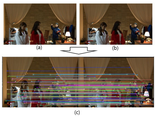
Figure 2.
Once the feature is extracted using SIFT from two adjacent images (a,b), feature matching between the images is carried out using RANSAC (c).
The actual experiment is carried out using all 25 images, as shown in Section 5. The better result of feature matching (including feature extraction) leads to greater simplicity, easiness, and the better quality of the depth map or synthesis result. Even though the images are rectified, since calibration is an optimization process, there is always the possibility of the existence of a small orientation between the images. Since the images are captured by cameras that are located at different positions with respect to each other, various scaling also exists, and this is different from the case of stereo vision (only a two-view system). Thanks to the robustness of the SIFT algorithm to scaling and rotation, the present work employs SIFT to extract the feature points from a set of images. Once feature matching is carried out among the images, the geometric relationship among the feature points is established. The relationship plays a key role in the synthesis of the images. Image synthesis using SIFT was proposed in [45], which only used 2D image points for stitching images. Homography estimation between two images is necessary to complete feature matching using the RANSAC algorithm. To find the homography between the images, the RANSAC algorithm randomly chooses sample feature points from the images. Based on the randomly chosen samples, the homography is estimated, then the homography is applied to the other feature points that were not sampled previously. If the estimated result is not correct, the random sampling procedure is carried out again, and the procedure is iterated until the accuracy of the estimation of the homography is satisfactory. Accurate homography can possibly lead to the better quality of the depth map estimation stitching result under the assumption that the images are in affine transformation. This paper aims to generate the synthesized 3D mesh and texture, so depth map estimation with high accuracy is also desired. Rectified images provide relative depth information using the disparity between the matched points. In other words, the vertical coordinates of the matched points in the images are equivalent once the rectification is completed. To generate the mesh, the depth should be calculated. Since the experiments in this work also use a set of images, the procedures of depth extraction are very similar to the stereo vision technique. Thus, the depth (z) is calculated using the baseline (b) (the distance between the optical centers of the cameras), the focal length of the camera (f), and the disparity (d) between two matched points and as follows.
where and are the horizontal 2D pixel coordinates of and , respectively, in the image plane (Figure 3).
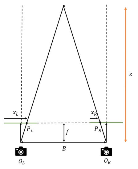
Figure 3.
Depth map estimation is carried out using the disparity value and based on the geometric relationship between two image planes.
The parallax between two images generates occlusion, where the disparity calculation is impossible, as shown in Figure 4. However, array cameras can mitigate this problem because there are other viewpoints that can alleviate the limitation of only the two-view system (stereo camera system).
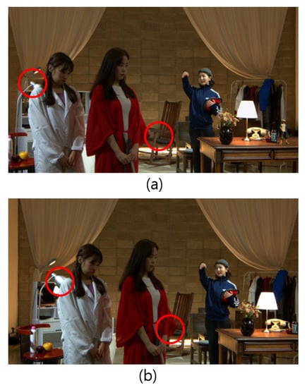
Figure 4.
Disparity estimation is performed by calculating the difference of the horizontal coordinates of two adjacent images (a,b). Disparity estimation is inaccurate or impossible to estimate due to the existence of occlusion (e.g., occlusion is observed in the areas of the red circles in (a,b).
Contrary to the usual stereo vision method, the present work uses 25 cameras, each of which is located at different positions, and accounts for the occlusion problem, which can be resolved because multiple (more than two) viewpoints are available. The number of viewpoints enables us to generate a depth map of reliable quality with 25 images.
3. Synthesis with Adaptive View Selection
The number of images to synthesize the images (both the color and depth images) influences the efficiency and accuracy when generating the depth map, mesh, texture, and synthesis results, and as expected, there exists a trade-off between accuracy and efficiency. This section presents the adaptive selection of the images for the extension of the depth map and color image by synthesizing arbitrary views. View synthesis is a difficult work because the synthesis procedure can result in errors in the overlapped region between images from different viewpoints that have the same image context. For example, given two images, the optimal cut region between the overlapped areas leads to a successful transition between the images. Due to the existence of overlapped regions that contain the same content, it is important to merge the images into a single image. Some images having common content are mapped onto the same region of the synthesized image. To solve this problem, blending the images is required when the synthesis is performed. The synthesis of the depth images that correspond to the color images acquired by the array cameras is more difficult than the synthesis of 2D color images, because depth synthesis has the additional problem of fewer feature points than those of color images. A successful synthesis result should avoid the discontinuities possibly contained in the result, so the synthesis work should fully exploit the image, the depth, and the relative positions of the cameras. This leads to emphasizing the importance of calibrating the cameras, which was already solved in the experimental setup in this paper. Using 25 rectified images, twenty-five corresponding depth maps were consequently generated by calculating the disparities between adjacent images. In this paper, to efficiently proceed with the synthesized 3D model, the synthesis of the depth image was also performed. Since the approach to the synthesis of the depth map is similar to the one for synthesizing RGB images, we start by synthesizing RGB images. Each image is captured by the ith camera , (), and . Specifically, includes the 2D image plane of the ith camera. Each 2D image plane is included in and forms the projected image of the 3D real-world scene. However, depth map synthesis is different from view (color image) synthesis in that the depth map image lacks feature points compared to the color images. Thus, prior to depth map synthesis, the registration between the color image and depth map is required. As mentioned above, the synthesis of depth images is a difficult task, but it is much more efficient to generate a synthesized 3D model than to generate a new depth map from the synthesized RGB images. For the synthesis, the geometric relationship with the depth image needs to be established. For the depth map resulting from the pairs of images captured by the cameras located at different positions, there also exists a geometric transformation between any pairs of depth images. Pairs of feature points between images that are matched are mapped to the same position in the depth map images. To achieve the registration result, of course, the feature matching and homography should be estimated with high accuracy. In addition to accurate homography and feature matching, the proper selection of images needs to be performed, i.e., selecting the best views for synthesis is required. Simply selecting the neighboring image for depth map generation and feature matching will lead to a low accuracy of registration and synthesis. Since all of the images in the array are independent of each other, the extension and smooth transition between any pair of images are crucial parts of the synthesis. Only selecting neighboring (or adjacent) images will not provide sufficient clues for quality improvement. As the cameras are already rectified, homography estimation does not affect the accuracy of vertical alignment. However, in this work, homography estimation provides information about the geometric relationship between any pair of images. This procedure is different from the usual homography estimation in the stereo vision system. Homography estimation can be written as:
where and are two-dimensional points represented using homogeneous coordinates in the image plane, and , respectively, and is the homography matrix that uniquely determines the geometric relationship between two images. The relationship written in Equation (3) also can be represented as:
where and are two-dimensional points in a homogeneous coordinates system, i.e., and , and is a transformation matrix, called similarity transformation. The relationship written in Equation (4) can also be represented as:
where is the relative rotation (in degrees or radians) between two images and and are the translation between two images in the horizontal and vertical directions, respectively. s is a scaling factor that does not affect the result of interest in this work (s can be set to one for simplicity). In this case, the images are already rectified, and is almost equal to zero. is rewritten as:
where is a identity matrix. Since the array cameras are used, the homography is estimated between any pair of images, represented as follows.
where represents the homography between the points and . One example of homography estimation is shown in Figure 5.
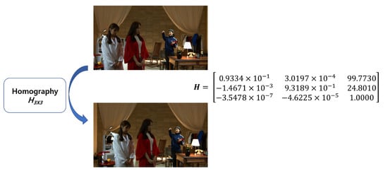
Figure 5.
One example of the homography matrix () estimation. Two images have relative positions, and homography estimation is one of the methods to represent the relationship.
Based on Equation (6), the relationship we chiefly deal with is the translation vector, . Since the images are rectified, all 25 images are translated one from the other. However, in the case of the array cameras of this work, different viewpoints generate scaling factors that are not constant. In other words, in Equation (7) has an element instead of s in Equation (6). Intuitively, as shown in Figure 6, the scaling of the objects in the images is different from each other.
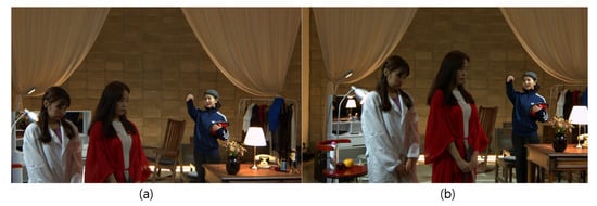
Figure 6.
If two images (a,b) have different scaling factors, the direct estimation of the disparity is impossible.
Due to the existence of scaling, even though the images are rectified, homography estimation is still necessary. In addition to insufficient feature points, depth images from all different viewpoints have different scales (see Figure 7), leading to the necessity of depth map compensation to achieve a reliable synthesis result.
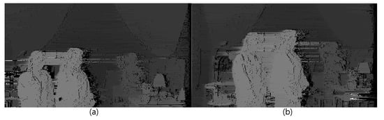
Figure 7.
Two images with different scaling factors can be appropriately depth mapped from each perspective if the scaling factor is accurately estimated. (a,b) are the depth maps of the images of Figure 6a,b, respectively.
The contents included in the images overlap each other, so the computational complexity of the synthesis work may be significantly increased. To achieve an efficient synthesis result, i.e., to decrease computational complexity, without information loss, the adaptive selection of the images is highly necessary. To reduce the computational complexity, depth estimation is performed using images of a reduced size, e.g., the image size is reduced to of the original one. The depth map result using the reduced size of the images did not show information loss in the experiments. In addition to reducing the size of the images, adaptive selection, i.e., sub-sampling of the images, is performed to significantly reduce the computational complexity. The adaptive selection is the most crucial part of this paper, and this contribution is different from the previous work on view synthesis. The flow diagram of the view selection proposed in this paper is depicted in Figure 8.
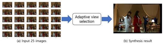
Figure 8.
Flow diagram of the proposed approach to view synthesis with adaptive view selection. (a) Input: 25 images. (b) Synthesized result using selected images.
As mentioned above, array cameras provide images that have overlapped contents. The overlapped contents provide sufficient information to synthesize the views. Prior to synthesis, feature points from each image are extracted, and the homography between the images is calculated after feature matching between them. All the images may not be necessary for the synthesis because all the images share common contents in the images. If image based rendering is of interest, the computational complexity is almost independent of the number of images. Intuitively, the use of fewer images can decrease the computational complexity because fewer images generate a smaller number of feature points, leading to less calculation for feature matching, as well as less calculation for depth information. Adaptive view selection (AVS), in this paper, provides a criterion for the selection of images (less than 25) that generate the view and depth map synthesis that does not degrade the general quality from a visual perspective. Let the result of the synthesis using all of the images (25) be defined by and the result of the synthesis using n images by , respectively; the goal of the determination of criterion is written as:
To achieve the determination of the criterion for view selection, three types of selection are presented. Each type of selection should contain the images that include all of the contents. In most cases of selection, the central image is used because the important contents of a target scene are contained in the central image. In the first, four-views selection is considered. Four-view selection randomly chooses four images among 25 images. This selection can decrease the computation time, but the amount of the overlapped region is smaller than the other cases if the images at the corners are selected. If we avoid the images at the corners, the synthesized result might not be able to cover the whole part of a scene. In this case, four images are selected, and they are located at the corners of the array, i.e., each of them is located at the left-bottom, right-bottom, left-top, and right-top (Section 5). Intuitively, four views can lose the information of all of the views contained in the array cameras. However, the selection of four images can be considered if they contain all the contents of a target scene. Of course, the parallax is bigger than any type of selection. As shown in the experimental results, four-view selection is vulnerable to information loss when synthesis is carried out. Due to the large parallax between any pairs of images, the insufficient results of feature matching can lead to the wrong homography estimation. To mitigate the large parallax, seven-view selection can be considered (Section 5). Seven-view selection decreases the amount of parallax compared to the one with four-view selection. The images at the corners and the image at the central position are added to the selection. Similar to the aforementioned selection, more images are selected so that the parallax can be decreased. Theoretically, the number of images selected can be from one to 25. However, if a larger number of images is selected, the computational complexity will increase. The quality of the synthesis can be saturated once the number of selected images is bigger than the threshold. This threshold can be determined based on the experiments here. Equation (8) can be rewritten as follows:
where is the threshold. Next, we discuss mesh generation and texture mapping with a synthesized color image and a depth image.
4. Mesh Generation and Texture Mapping
Synthesized depth images and color images generate a new 3D model with meshes and textures. In the previous section, we discussed the synthesis of depth and color images based on a geometric transformation between any pairs of images (color and depth). Thus, a set of color images (), depth images (), and a triangular mesh () contain the geometric transformation as follows.
where , , and represent the geometric transformation of color images, depth images, and triangles, respectively. To reconstruct the 3D structure of a scene of interest, two main approaches can be employed: one is using geometric reconstruction, and the other one is image based reconstruction. In the course of the geometric reconstruction, the 3D coordinates or a triangular mesh are widely used. The geometric 3D coordinate information can be represented using a triangular mesh, a binary volume depth-per-pixel, or other types of polygonal mesh [46,47,48]. Based on the depth map estimated using the parallax between neighboring views and using Delaunay triangulation, a 3D mesh is generated from the reference depth information. The pixel based mesh is generated based on the depth values, each of which is defined on each pixel, i.e., depth is assigned to each pixel. The polygon based mesh is generated on each polygon (a triangle in this paper) that is generated using triangulation. Feature points are extracted using SIFT from all of the images, and these points play the role of seed points to generate the Delaunay triangle (Figure 9).
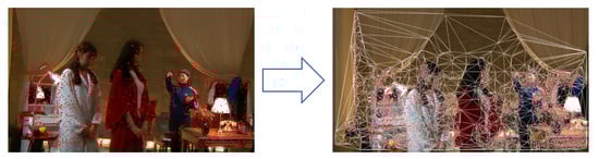
Figure 9.
A Delaunay triangle is generated followed by feature extraction. Triangulation (right image) is generated based on feature extraction (left image).
Prior to feature extraction, images are preprocessed using a low-pass filter. In this work, a bilateral filter is employed because it preserves the high frequency components of the image compared to the Gaussian filter (Figure 10).
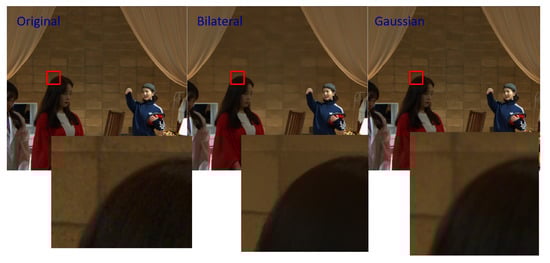
Figure 10.
The bilateral filter preserves the high frequency components of the images.
Once feature extraction has been performed, the result applies to generating the Delaunay triangle and to depth map generation. Both of them are necessary for mesh generation. Since the mesh contains 3D geometric information, a high quality depth map is required. In this work, the segmentation based depth map is employed [49]. Prior to calculating the disparity between matched feature points, mean-shift based segmentation is carried out. To resolve the occlusion problem inherent to depth map estimation, the gradient of the images is calculated to detect occlusion areas. By calculating the gradient of the image across the horizontal direction for the pair of matched points, occlusion can be detected. Once the gradient based detection is performed, the region of occlusion is finally detected based on the matching cost calculated using Equation (13). To improve the quality of synthesis, occlusion detection is required.
where , , , , m, and n are the coordinate points of and , the amount of shift in the horizontal and vertical direction, respectively. W is the size of the window to calculate the cost (dissimilarity). In addition to resolving occlusion, a depth map is generated corresponding to each image (Figure 11).
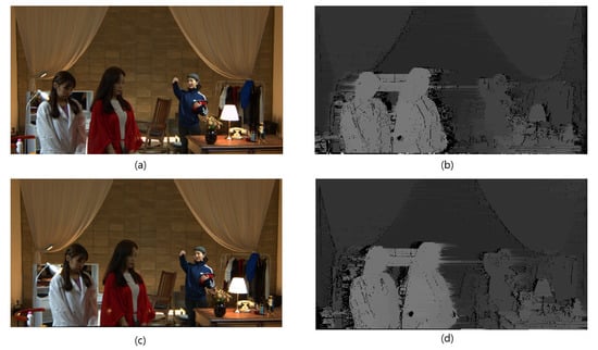
Figure 11.
Segmentation based depth map estimation. (a,c) Input images; (b) depth map corresponding to image (a); (d) depth map corresponding to image (c).
The depth map and the Delaunay triangles are combined to generate the 3D mesh. The third coordinate (depth information) is added to the generated triangles defined in the 2D coordinates so that the 3D mesh can be constructed (Figure 12).
Figure 12.
Depth map information is added to the triangle to generate the mesh. (a) Input image. (b) Depth map of image (a). (c) The generated triangular mesh.
Texture mapping can be accomplished by laying the color image on a three-dimensional space. The generated mesh yields a one-to-one mapping to the 2D color information from the 3D mesh result. In texture mapping, registration between the depth map, mesh, and RGB images should be performed because the mesh is an approximated depth map, and the blending of the color images needs to be carried out. The pixel coordinates of the color images should correspond to the coordinates of the depth map and the mesh. Adaptive view selection plays key role in the result of texture mapping because the desired scene should be represented in the 3D reconstruction result with the mesh and texture. To achieve proper view selection, occlusion should be dealt with prior to texture mapping. The results of the texture mapping are shown in Figure 13. The captured images are used to estimate the depth map, and the feature points are used to generate the Delaunay triangles. In addition to the depth map and the triangles, color information is added to them to generate the 3D view with the 3D mesh.
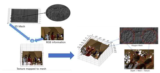
Figure 13.
Texture is mapped to the points, the locations of which are matched to those of the generated mesh.
To generate the synthesized 3D mesh with texture, we fully utilize the synthesized color and depth images. The synthesis of the depth images is performed based on the establishment of the scaling, rotation, and translation between any pair of depth images. This approach is more efficient than the approach that generates a new depth map from a synthesized color image.
5. Experimental Results
In order to substantiate our proposed AVS method, experimental results are presented with images captured by 25 array cameras, i.e., the dataset contains 25 images. Simulations were performed using Python 3.7.4, Numpy 1.16.4, Matplotlib 3.1.0, and mpl-toolkits 1.2.1 and were performed on a CPU Intel® Core™ i3-8100@3.60 GHz, GPU Geforce 270 RTX, with 24 GB RAM. This section evaluates the proposed approach for AVS in a quantitative and qualitative way. Specifically, the effect of the number of images used for synthesis, mesh generation, and texture mapping is investigated. In the experiments, the number of selected images for the synthesis varied from four images to 25 images, and the computational complexity (efficiency) and PSNR (quality) were measured. All images were captured by array cameras with a array structure. Figure 8 shows the input images. In this work, we used a real-world scene composed of various objects rather than using a single object in a totally controlled circumstance, as the existing work. To this end, the optimal number of images for the synthesis of 3D modeling was determined from the experiments. The synthesis results of the image and depth map with different numbers of input images were evaluated. The cameras were already rectified, so the implementation started with the disparity calculation. Figure 14 shows one example result of the synthesis of the 2D images using 25 views. If all 25 images were used for view synthesis, the result would show the extended range of views in the vertical and horizontal direction (Figure 14). All of the experiments were performed using images of pixels, and the size of the images was downsized (to ) when the depth was estimated, for computational efficiency.
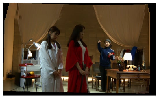
Figure 14.
View synthesis with 25 images is extended in the vertical and horizontal direction.
The quality of the synthesis using 25 images can be improved if the overlapped regions can be more accurately detected and more accurate homography estimation is performed. The improved results are shown in Figure 15.
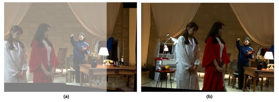
Figure 15.
The results of the synthesized images is improved with accurate homography estimation in addition to accurate detection of the overlapped regions. (a) Synthesis before homography optimization. (b) Synthesis with homography optimization.
Next, the view and depth map synthesis with adaptive view selection is depicted. As expected, the increase of the selected images provides a better quality synthesis result with higher computational complexity. In this experiment, we need to find the optimal number of selected views that does not significantly degrade the quality of the synthesis results. To generate the synthesized 3D model, the number of feature points used was ranged from 800 to 1000 (in the case of selecting 4 images: 827, in the case of selecting 7 images: 885, in the case of selecting 11 images: 807, in the case of selecting 25 images: 914). In other words, even if the selected number of images varied, the variation of the number of extracted feature points was not large. As a result, even if seven or 11 images were selected, the synthesis result would not lose generality. In other words, only a 50 percent sampling rate or less than this rate sufficiently provided a reliable synthesis result from the visual perspective. If four views were selected, the synthesis result showed errors in that the objects were overlapped in the wrong positions in the image plane (Figure 16). As shown in the results below, the results of the synthesis using different numbers of images provided different qualities. However, since different views were synthesized, the extended depth map and image were generated.
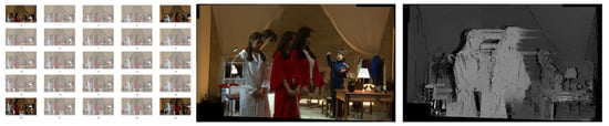
Figure 16.
View synthesis with four images is extended in the vertical and horizontal direction.
If 7, 11, and 25 views were selected, the synthesis result showed better quality than the one with four views (Figure 17, Figure 18 and Figure 19).
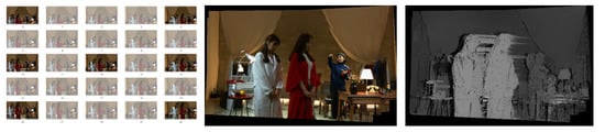
Figure 17.
View synthesis with seven images is extended in the vertical and horizontal direction.
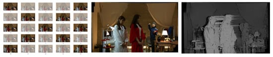
Figure 18.
View synthesis with 11 images is extended in the vertical and horizontal direction.
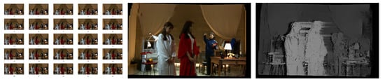
Figure 19.
View synthesis with 25 images is extended in the vertical and horizontal direction.
The quality of the results was validated using the results from the visual perspective (quantitative) and using the PSNR. The quality of the synthesized results with different numbers of images is shown in Figure 20.
where is the maximum intensity value of the synthesized image and is mean squared error calculated between the synthesized and the original image.
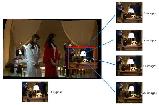
Figure 20.
View synthesis with different numbers of images shows that the quality with seven or 11 images is competitive with the one with 25 images.
As shown in Table 1, the PSNR of the synthesized results validates the efficiency of the proposed method in that the PSNR of the results with seven and 11 images is more competitive than the result with 25 images. The relative quantity using the percentage is also provided in Table 1 (in the last column). The computational complexity (seconds) is shown in Table 1 and Figure 21. The execution time significantly increased when 25 images were used to generate the results, but the quality (PSNR) was very competitive to the case of using 11 images. The selection of views was randomly carried out. For example, Figure 17 shows one example of seven selected views. The execution time almost increased exponentially with the number of images selected. All the experiments were conducted on a 3.00 GHz (6 CPUs) Intel(R) Core(TM) i5-8500 processor and 8GB-RAM workstation.

Table 1.
Computation time (s) with the number of images used for synthesis.
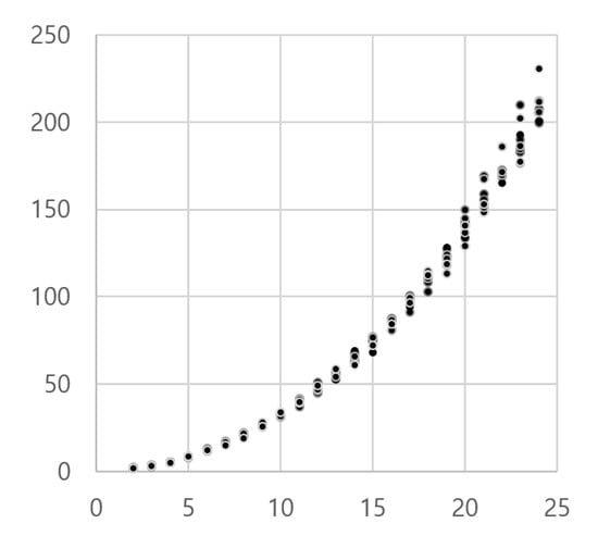
Figure 21.
Selection of images is randomly chosen among the 25 images. As the number of images is selected, the computational complexity increases accordingly. Computational complexity is represented using time (seconds), and the horizontal axis represents the number of selected images ().
The triangulation result and depth map were combined to synthesize the depth map itself so that we could generate the 3D synthesis result (Figure 22).
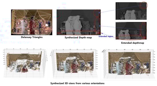
Figure 22.
View synthesis with four images is extended in the vertical and horizontal direction.
6. Conclusions
This paper presents an approach for the efficient 3D representation of a real-world scene using mesh and texture mapping. In particular, this work presents AVS, which determines the optimal number of images that can provide a reliable result of the extended 3D view without considerable loss of quality. This work analyzes the computational complexity and image quality by varying the number of images. The selection of images is carried out based on the contents included in the images for a full coverage. Since 3D rendering or 3D reconstruction work sacrifices computational efficiency due to the size of the images, the present work chiefly deals with efficiency and simplicity. Of course, accurate 3D reconstruction is very important; however, limited resources such as high cost hardware or the size of devices lead to considering realistic aspects. This work starts from generating the depth map of all of the images and feature extraction to generate the 3D mesh. To this end, this work proposes an approach to the synthesis of images and depth map images (in gray-scale) with the AVS approach. This work is different from the existing work in that this work synthesizes not only 2D images, but also gray-scale depth map images and uses both of them to alleviate the limitations: 2D images lack depth information, and depth maps lack feature points. Registration between the depth map and color image is carried out to generate the synthesized image and depth map. With the synthesized depth map, the texture is mapped onto the extended depth map. Depth map synthesis is a challenging problem because only the depth map lacks feature points compared to the amount of feature points in a color image. This work still has limitations in that it depends on the quality of depth estimation. Future work will focus on developing a framework for 3D view synthesis based on the deep neural network.
Author Contributions
Conceptualization, G.K. and D.L.; methodology, G.K.; validation, G.K. and D.L.; formal analysis, G.K. and D.L.; investigation, G.K. and D.L.; data curation, G.K. and D.L.; writing—original draft preparation, G.K.; writing—review and editing, D.L.; visualization, G.K. and D.L.; supervision, D.L.; project administration, D.L.; funding acquisition, D.L. All authors have read and agreed to the published version of the manuscript.
Funding
This work was partly supported by the Institute for Information & communications Technology Promotion (IITP) grant funded by the Korean government (MSIT) (2016-0-00564, Development of Intelligent Interaction Technology Based on Context Awareness and Human Intention Understanding) and was supported by the Basic Science Research Program through the National Research Foundation of Korea (NRF) funded by the Ministry of Science, ICT & Future Planning (2019R1G1A110017212).
Institutional Review Board Statement
Not applicable.
Informed Consent Statement
Not applicable.
Data Availability Statement
Data available on request due to privacy. The data presented in this study are available on request from the corresponding author.
Conflicts of Interest
The authors declare no conflict of interest.
References
- Pnner, E.; Zhang, L. Soft 3D reconstruction for view synthesis. ACM Trans. Graph. 2017, 36, 1–11. [Google Scholar] [CrossRef]
- Nguyen, T.-N.; Huynh, H.-H.; Meunier, J. 3D Reconstruction With Time-of-Flight Depth Camera and Multiple Mirrors. IEEE Access 2018, 6, 38106–38114. [Google Scholar] [CrossRef]
- Fickel, G.P.; Jung, C.R. Disparity map estimation and view synthesis using temporally adaptive triangular meshes. Comput. Graph. 2017, 68, 43–52. [Google Scholar] [CrossRef]
- Huang, H.-P.; Tseng, H.-Y.; Lee, H.-Y.; Huang, J.-B. Semantic View Synthesis. In Computer Vision—ECCV 2020, Proceedings of the European Conference on Computer Vision, Glasgow, UK, 23–28 August 2020; Springer: Cham, Switzerland, 2020; pp. 592–608. [Google Scholar]
- Attal, B.; Ling, S.; Gokaslan, A.; Richardt, C.; Tompkin, J. MatryODShka: Real-time 6DoF Video View Synthesis Using Multi-sphere Images. In Computer Vision—ECCV 2020, Proceedings of the European Conference on Computer Vision, Glasgow, UK, 23–28 August 2020; Springer: Cham, Switzerland, 2020; pp. 441–459. [Google Scholar]
- Luo, G.; Zhu, Y.; Li, Z.; Zhang, L. A Hole Filling Approach Based on Background Reconstruction for View Synthesis in 3D Video. In Proceedings of the IEEE Conference on Computer Vision and Pattern Recognition, Las Vegas, NV, USA, 27–30 June 2016; pp. 1781–1789. [Google Scholar]
- Stoko, P.; Krumpen, S.; Hullin, M.B.; Weinmann, M.; Klein, R. SLAMCast: Large-Scale, Real-Time 3D Reconstruction and Streaming for Immersive Multi-Client Live Telepresence. IEEE Trans. Vis. Comput. Graph. 2019, 25, 2102–2112. [Google Scholar] [CrossRef]
- Li, Y.; Claesen, L.; Huang, K.; Zhao, M. A Real-Time High-Quality Complete System for Depth Image-Based Rendering on FPGA. IEEE Trans. Circuits Syst. Video Technol. 2019, 29, 1179–1193. [Google Scholar] [CrossRef]
- Lazaros, N.; Sirakoulis, G.C.; Gasteratos, A. Review of Stereo Vision Algorithms: From Software to Hardware. Int. J. Optomechatron. 2008, 2, 435–462. [Google Scholar] [CrossRef]
- Hartely, R.; Zisserman, A. Multiple View Geometry in Computer Vision, 2nd ed.; Cambridge University Press: Cambridge, UK, 2004. [Google Scholar]
- Geng, J. Structured-light 3D surface imaging: A tutorial. Adv. Opt. Photonics 2011, 3, 128–160. [Google Scholar] [CrossRef]
- Jeught, S.; Dirckx, J. Real-time structured light profilometry: A review. Opt. Lasers Eng. 2016, 87, 18–31. [Google Scholar] [CrossRef]
- Tsai, R. A versatile camera calibration technique for high accuracy 3D machine vision metrology using off-the-shelf TV cameras and lenses. IEEE J. Robot. Autom. 1987, 3, 323–344. [Google Scholar] [CrossRef]
- Zhang, Z. A flexible new technique for camera calibration. IEEE Trans. Pattern Anal. Mach. Intell. 2000, 22, 1330–1334. [Google Scholar] [CrossRef]
- Heikkila, J. Geometric camera calibration using circular control points. IEEE Trans. Pattern Anal. Mach. Intell. 2000, 22, 1066–1077. [Google Scholar] [CrossRef]
- Rocco, I.; Cimpoi, M.; Arandjelović, R.; Torii, A.; Pajdla, T.; Sivic, J. Neighbourhood Consensus Networks. In Proceedings of the 32nd Conference on Neural Information Processing Systems (NeurIPS 2018), Montreal, QC, Canada, 3–8 December 2018; pp. 1–12. [Google Scholar]
- Jeon, H.-G.; Lee, J.-Y.; Im, S.; Ha, H.; Kweon, I. Stereo Matching With Color and Monochrome Cameras in Low-Light Conditions. In Proceedings of the IEEE Conference on Computer Vision and Pattern Recognition, Las Vegas, NV, USA, 27–30 June 2016; pp. 4086–4094. [Google Scholar]
- Smolyanskiy, N.; Kamenev, A.; Birchfield, S. On the Importance of Stereo for Accurate Depth Estimation: An Efficient Semi-Supervised Deep Neural Network Approach. In Proceedings of the IEEE Conference on Computer Vision and Pattern Recognition (CVPR) Workshops, Salt Lake City, UT, USA, 18–22 June 2018; pp. 1007–1015. [Google Scholar]
- Zhang, S. High-speed 3D shape measurement with structured light methods: A review. Opt. Lasers Eng. 2018, 106, 119–131. [Google Scholar] [CrossRef]
- Su, S.; Heide, F.; Wetzstein, G.; Heidrich, W. Deep End-to-End Time-of-Flight Imaging. In Proceedings of the IEEE Conference on Computer Vision and Pattern Recognition, Salt Lake City, UT, USA, 18–22 June 2018; pp. 6383–6392. [Google Scholar]
- Ha, M.; Xiao, C.; Pham, D.; Ge, J. Complete grid pattern decoding method for a one-shot structured light system. Appl. Opt. 2020, 59, 2674–2685. [Google Scholar] [CrossRef] [PubMed]
- Gu, F.; Cao, H.; Song, Z.; Xie, P.; Zhao, J.; Liu, J. Dot-coded structured light for accurate and robust 3D reconstruction. Appl. Opt. 2020, 59, 10574–10583. [Google Scholar] [CrossRef] [PubMed]
- Flores, J.L.; Ayubi, G.A.; Martino, J.; Castillo, O.; Ferrari, J. 3D-shape of objects with straight line-motion by simultaneous projection of color coded patterns. Opt. Commun. 2018, 414, 185–190. [Google Scholar] [CrossRef]
- Li, D.; Xu, F.; Wang, Y.; Wang, H.; Wu, C.; Zhou, F.; Song, J. Lasers structured light with phase-shifting for dense depth perception. Results Phys. 2019, 14, 102433. [Google Scholar] [CrossRef]
- Tang, S.; Zhang, X.; Song, Z.; Song, L.; Zeng, H. Robust pattern decoding in shape-coded structured light. Opt. Lasers Eng. 2017, 96, 50–62. [Google Scholar] [CrossRef]
- Gandhi, V.; Čech, J.; Horaud, R. High-resolution depth maps based on TOF-stereo fusion. In Proceedings of the IEEE International Conference on Robotics and Automation, Saint Paul, MN, USA, 14–18 May 2012; pp. 4742–4749. [Google Scholar]
- Marin, G.; Zanuttigh, P. Reliable Fusion of ToF and Stereo Depth Driven by Confidence Measures. In Computer Vision—ECCV 2016, Proceedings of the European Conference on Computer Vision, Glasgow, UK, 11–14 October 2016; Springer: Cham, Switzerland, 2016; pp. 386–401. [Google Scholar]
- Marwah, K.; Wetzstein, G.B.; Veeraraghavan, A.; Raskar, R. Compressive Light Field Photography. ACM Trans. Graph. 2013, 32, 1–12. [Google Scholar] [CrossRef]
- Ihrke, I.; Restrepo, J.; Mignard-Debise, L. Principles of Light Field Imaging: Briefly revisiting 25 years of research. IEEE Signal Process. Mag. 2016, 33, 59–69. [Google Scholar] [CrossRef]
- Yamaguchi, M. Light-field and holographic three-dimensional displays [Invited]. J. Opt. Soc. Am. A 2016, 33, 2348–2364. [Google Scholar] [CrossRef]
- Levoy, M.; Hanrahan, P. Light field rendering. In SIGGRAPH ’96, Proceedings of the 23rd Annual Conference on Computer Graphics and Interactive Techniques, New Orleans, LA, USA, 4–9 August 1996; Association for Computing Machinery: New York, NY, USA, 1996; pp. 31–421. [Google Scholar]
- Levoy, M.; Nr, R.; Adams, A.; Footer, M.; Horowitz, M. Light field microscopy. In SIGGRAPH ’06: ACM SIGGRAPH 2006 Papers; Association for Computing Machinery: New York, NY, USA, 2006; pp. 924–934. [Google Scholar]
- Jeon, H.-G.; Park, J.; Choe, G.; Park, J.; Bok, Y.; Tai, Y.-W.; Kweon, I. Accurate Depth Map Estimation From a Lenslet Light Field Camera. In Proceedings of the IEEE Conference on Computer Vision and Pattern Recognition, Boston, MA, USA, 7–12 June 2015; pp. 1547–1555. [Google Scholar]
- Overbeck, R.; Erickson, D.; Evangelakos, D.; Pharr, M.; Debevec, P. A system for acquiring, processing, and rendering panoramic light field stills for virtual reality. ACM Trans. Graph. 2018, 37, 1–15. [Google Scholar] [CrossRef]
- Cho, D.; Lee, M.; Kim, S.; Tai, Y.-W. Modeling the Calibration Pipeline of the Lytro Camera for High Quality Light-Field Image Reconstruction. In Proceedings of the IEEE International Conference on Computer Vision (ICCV), Sydney, Australia, 8–12 April 2013; pp. 3280–3287. [Google Scholar]
- Shewchuk, J.R. Delaunay refinement algorithms for triangular mesh generation. Comput. Geom. 2002, 22, 21–74. [Google Scholar] [CrossRef]
- Broxton, M.; Flynn, J.; Overbeck, R.; Erickson, D.; Hedman, P.; Duvall, M.; Dourgarian, J.; Busch, J.; Whalen, M.; Debevec, P. Immersive light field video with a layered mesh representation. ACM Trans. Graph. 2020, 39, 1–15. [Google Scholar] [CrossRef]
- Cserkaszky, A.; Barsi, A.; Kara, P.; Martini, M. To interpolate or not to interpolate: Subjective assessment of interpolation performance on a light field display. In Proceedings of the IEEE International Conference on Multimedia & Expo Workshops (ICMEW), Hong Kong, China, 10–14 July 2017; pp. 55–60. [Google Scholar]
- Kalantari, N.K.; Wang, T.C.; Ramamoorthi, R. Learning-based view synthesis for light field cameras. ACM Trans. Graph. 2016, 35, 1–10. [Google Scholar] [CrossRef]
- Heber, S.; Pock, T. Convolutional Networks for Shape from Light Field. In Proceedings of the IEEE Conference on Computer Vision and Pattern Recognition, Las Vegas, NV, USA, 27–30 June 2016; pp. 3746–3754. [Google Scholar]
- Jeon, H.-G.; Park, J.; Choe, G.; Park, J.; Bok, Y.; Tai, Y.-W.; Kweon, I. Depth from a Light Field Image with Learning-Based Matching Costs. IEEE Trans. Pattern Anal. Mach. Intell. 2019, 41, 297–310. [Google Scholar] [CrossRef]
- Henman, P.; Ritschel, T.; Drettakis, G.; Brostow, G. Scalable inside-out image-based rendering. ACM Trans. Graph. 2016, 35, 1–11. [Google Scholar]
- Luo, B.; Xu, F.; Richardt, C.; Yong, J.-H. Parallax360: Stereoscopic 360∘ Scene Representation for Head-Motion Parallax. IEEE Trans. Vis. Comput. Graph. 2018, 24, 1545–1553. [Google Scholar] [CrossRef]
- Tareen, S.; Sallem, Z. A comparative analysis of SIFT, SURF, KAZE, AKAZE, ORB, and BRISK. In Proceedings of the International Conference on Computing, Mathematics and Engineering Technologies (iCoMET), Sukkur, Pakistan, 3–4 March 2018; pp. 1–10. [Google Scholar]
- Brown, M.; Lowe, D.G. Automatic Panoramic Image Stitching using Invariant Features. Int. J. Comput. Vis. 2007, 74, 59–73. [Google Scholar] [CrossRef]
- Riegler, G.; Ulusoy, A.S.; Geiger, A. OctNet: Learning Deep 3D Representations at High Resolutions. In Proceedings of the IEEE Conference on Computer Vision and Pattern Recognition (CVPR), Honolulu, HI, USA, 21–26 July 2017; pp. 3577–3586. [Google Scholar]
- Whitaker, R.T. Reducing Aliasing Artifacts in Iso-Surfaces of Binary Volumes. In Proceedings of the 2000 IEEE Symposium on Volume Visualization (VV 2000), Salt Lake City, UT, USA, 9–10 October 2000; pp. 23–32. [Google Scholar]
- Liu, C.; Sang, X.; Yu, X.; Gao, X.; Liu, L.; Wang, K.; Yan, B.; Yu, C. Efficient DIBR method based on depth offset mapping for 3D image rendering. In AOPC 2019: Display Technology and Optical Storage; International Society for Optics and Photonics: Bellingham, WA, USA, 2019; pp. 1–7. [Google Scholar]
- Kim, J.; Park, C.; Lee, D. Block-Based Stereo Matching Using Image Segmentation. J. Korean Inst. Commun. Inf. Sci. 2019, 44, 1402–1410. [Google Scholar]
Publisher’s Note: MDPI stays neutral with regard to jurisdictional claims in published maps and institutional affiliations. |
© 2021 by the authors. Licensee MDPI, Basel, Switzerland. This article is an open access article distributed under the terms and conditions of the Creative Commons Attribution (CC BY) license (http://creativecommons.org/licenses/by/4.0/).