A Dynamic Conflict Analysis Method for EW Effectiveness Evaluation Based on Conditional State Space

Abstract

An Electronic Warfare (EW) system is a highly complex and highly uncertain dynamic system. With a change of environment conditions, EW systems present different states and exhibit the characteristics of a Markov chain, which also directly affects and determines the effectiveness of EW systems. In order to describe and solve the problem of evaluating the effectiveness of EW, based on the definition of EW conflict system, this paper analyses the dynamic relationship of state between target unit and task unit of an EW system, studies the measurability of state, obtains measurable state space, then introduces randomness into state space and gives the theory, properties and applications of the state random process, state Markov process. Finally, the dynamic conflict analysis model of EW effectiveness is constructed and used to analyze the state transition process in the dynamic conflict process of an EW system, which is of great value to improve the theoretical system of EW effectiveness evaluation.

1. Introduction

The study of military problems can start from both qualitative and quantitative aspects, and the key to the quantitative analysis of military problems is to investigate the operational effectiveness of operational operations and weapons systems. In recent years, electronic warfare (EW), as an important means of warfare in modern warfare, has developed from the confrontation between single systems and single platforms to the systematic confrontation between opposing parties in the whole time domain and full frequency domain of warfare space. To this end, how to make better use of the power of EW, better organize the operations of EW, and better play its effectiveness and role are the key issues that are concerned about and studied by all military powers in the world today.

An EW system’s effectiveness is defined as the degree to which it can meet the desired objectives in an operational situation [1]. It is a multi-dimensional description of EW capability, and is the essential basis to demonstrate, develop, plan and configure the EW system. It is also the most important comprehensive index to evaluate the merits of EW system and an important way to judge the operational capability of EW systems.

EW effectiveness evaluation is the evaluation and estimation of the degree. Since the last century to the present, the international EW professionals have done a lot of work on the subject of EW effectiveness analysis, and have achieved remarkable results, which lays a foundation for the systematic and comprehensive research on the EW effectiveness analysis and evaluation. In Ref. [2], it first summarized the effectiveness analysis/evaluation method of EW that have appeared at that time, and elaborated the necessity of the EW effectiveness analysis. The effects of electronic jamming on search/warning radar, tracking radar and communication equipment are introduced in detail, and the research methods of EW simulation test to evaluate the quality of jamming effect of jamming signal style or inherent potential of electronic jamming are evaluated. In Ref. [3], by discussing the influence of electronic jamming on the ability of radar detection to find targets and the reduction of radar detection distance caused by barrage noise jamming, the concept of radar burn through distance is first proposed. The reduction degree of airborne surveillance radar capability in the presence of jamming or not was evaluated in [4]. The relationship between various radar anti-jamming measures and various electronic countermeasure measures using ECCM-ECM relationship matrix description has been described in [5,6,7]. In Refs. [8,9,10], radar effectiveness evaluation index system is divided into three sublayers: radar intrinsic performance, radar anti-jamming performance and electromagnetic environment index. Radar intrinsic performance indicators mainly include radar transmission power, radar antenna gain, detection distance under jamming-free conditions, detection probability under jamming-free conditions, and so on. The anti-jamming performance index of radar mainly considers the degree of change of each performance index under the jamming condition, such as suppression factor, relative burn-through distance, anti-jamming quality factor and anti-jamming improvement factor. The electromagnetic environment index mainly involves the choice of jamming time, the signal flow density of the electromagnetic environment, and so on. In Ref. [11] believes that in the actual operational environment, it is impossible for the interfering party to obtain too many evaluation parameters directly from the hostile target, but the evaluation algorithm must be able to meet the rapid adaptation of the interference to the environment and the change of the states of the opposing target. In order to improve the efficiency of jamming effectiveness evaluation, artificial intelligence, neural network and other algorithms can be introduced into the jamming effectiveness evaluation to get the function relationship between the jamming strategy and the jamming effectiveness value in a certain environment.

Generally, the typical EW effectiveness evaluation modes can be divided into two categories: (1) carrying out system structure analysis and establishing evaluation model from the EW system itself; (2) based on the tactical use effect of the EW system, analyzing the impact of the implementation of electronic interference on the target equipment system of the interfered object, and establishing the model. These two modes are mainly based on the measurement of EW operational effect, and the combination of EW countermeasure features is insufficient. Especially with the evolution of the war form, the improvement of the EW system, the factors that affect the effectiveness of EW are becoming more and more complex. The traditional evaluation mode exposes many problems and deficiencies such as the fuzziness of the concept of the effectiveness of EW, the diversity of index measures, the confusion of model establishment, and so on, which make it difficult to effectively evaluate the effectiveness of EW.

EW includes non-cooperative conflict confrontation among multiple unit systems and levels. Considering that there are many uncertainties in the system states of the two hostile parties, it is difficult to quantify the system state completely, which is the crux of the problem of EW effectiveness evaluation. The key to quantify the state is the index. There are many indexes to evaluate the effectiveness of EW. It is an important purpose to select and quantify the system state reasonably in a large number of attribute characteristic indexes so as to determine the appropriate states of EW. In this way, the EW effectiveness evaluation problem can be abstracted into a multi condition attribute states evaluation problem. In Ref. [12], in order to reflect the law of state change and the dynamic characteristics of signals within the system, the system is equivalent to a finite state machine, and a hidden Markov model is used for modeling and analysis. In Ref. [13], based on the interaction relationship between radar and EW, the main basis of online evaluation of jamming effect based on the jammer’s reconnaissance radar signal is analyzed. Then, the implementation process of online evaluation method of jamming effect is given by establishing the mapping relationship between the change of radar working state and the jamming effect, and combining with the recognition of radar attributes and state.

For the EW system, its condition attribute states itself has strong randomness, fuzziness, incompleteness, imprecision, inconsistency, instability and differences, causing that the factors affecting the effectiveness of EW cannot be fully understood, while they behave the combination of qualitative and quantitative information. As a result, a distinct gray feature between the states can be observed. Grey correlation analysis analyses the uncertain correlation among things, quantitatively analyses the degree of correlation among various factors, and finally obtains the degree of correlation between system effectiveness and related indicators, to make a judgment on its position in the system. The Grey theory can comprehensively evaluate multi-target and multi-factor complex EW systems under the circumstance of insufficient information of EW, and provide richer evaluation information than other methods [14,15]. However, the application of Grey correlation in effectiveness evaluation is mostly based on the idea of ideal projection. In particular, using positive ideal evaluation matrix and negative ideal evaluation matrix as reference [16], it is easy to ignore the impact of the excellence of local indicators. Besides, the values of positive ideal evaluation matrix or negative ideal evaluation matrix are often too extreme in decision-making, and decision makers tend to set a more rational expectation. In addition, EW effectiveness evaluation involves a large amount of feature information including both self-characteristics and target attributes. It is difficult to build a model that considers all factors based on the relationship between features. In this way, the EW effectiveness evaluation problem can be more specific to a multi-condition attribute states evaluation problem with fuzzy and random characteristics.

In the process of effectiveness evaluation, due to fuzziness and randomness, different conditional attribute states may make the EW system meet the requirements. But according to the definition [1], when multiple EW systems meet the required objectives in the same operational situation, the system effectiveness is consistent, which is obviously not conducive to assist decision-making by evaluation. From this point of view, in order to further evaluate the effectiveness of EW scientifically, three key descriptive problems needed to be solved for the effectiveness evaluation of EW are decomposed:

Question 1: How to define the desired objectives?

Question 2: How to describe the operational situation of EW?

Question 3: How to measure the degree to which the operational situation meets the desired objectives?

Clearly, there is a conflict between the actual operational situation of EW and the degree of desired objectives. Desired objectives and actual operational situations largely depend on the mastery of the target unit and the capability of the task unit system, while satisfaction depends on the degree of conflict between the desired objectives and the actual operational situations [8]. Conflicts in the EW system also directly leads to the complexity of decision-making problems in the application process of EW, and become the focus and core issue in the study of the effectiveness of EW. Conflict decision-making problems in EW are complex in structure and computation. The structure complexity refers to the complexity of the components and their relationships of the EW problem, which is manifested by the poor structure of the problem, the ambiguous goal of the problem, the changeability of the relationship and so on. Literature [17] indicates that the structure of the problem is related to the representability of the problem, and that the weak structure problem cannot be accurately represented as a benign structure problem, mainly because the possible state and the transformation between states of the problem are unknown. Because of the uncertainty caused by the non-cooperative confrontation, so this paper defines the problem of EW conflict as a problem of accurate representation of weak structure. Further, the core of the conflict problem of EW becomes the representation and transfer of the conflict state of EW.

Currently, scholars have studied the conflict problem as a kind of independent problem, and proposed conflict analysis methods such as F-H analysis method [18,19], graph model [20,21,22], and conflict resolution method [23,24] based on rough set. Among them, the conflict analysis method of rough set is an extension of the conflict analysis graph model [25], which can more effectively describe and solve conflict problems, especially multi-conflict problems. A large number of conflict analysis mainly focus on description, portraying conflict problems and building conflict models. The conflict information system in the model is a static information system, which provides too abstract conflict information to effectively describe the real conflict problems and find a feasible set of strategies in the system. Especially for the EW, which needs more conflict enhancement than conflict reduction, it is necessary to effectively describe the dynamic change of the conflict state of the EW system, analyze the state transition process of the EW conflict system, and predict the possible trend of the conflict so as to take appropriate strategies.

At present, few papers systematically study the effectiveness of EW from the perspective of state conflict. The Markov Chain Monte Carlo (MCMC) method is an effective state processing method, which fully considers the relationship between system status [26]. Based on the characteristics of the state presented by the EW conflict system over time, this paper first analyses the dynamic relationship between the state of the target unit and the task unit of the EW system by studying the conflicts in the EW system. Secondly, on the basis of studying the measurability of condition state attributes between target units and task units of the EW conflict system, the measurable state space of EW effectiveness is established by referring to the multidimensional holistic analysis strategy in the spatial analysis method [27]. Then, introducing randomness into the state space, the Markov transition process of the conflict state of EW is analyzed, and the probability matrix of state transition and related properties are given. Finally, a dynamic conflict analysis model for EW effectiveness is constructed based on the Grey Relation Analysis of conflict states. The static and dynamic correlation characteristics are analyzed during the conflict states of EW, and the availability of the method is verified by an example.

2. Formal Definition of EW Conflict State

This section mainly solves the problem of modeled description of the system. First, the EW Task Unit System and the EW Target Unit System are unified and defined as the EW Conflict System. Secondly, the relationship between system elements is hierarchically analyzed to find the nature of the conflict. Finally, conflict relationships between systems are mapped to conflicts between states to achieve a mapping description from system to state.

2.1. EW Conflict System

EW is a set of measures and actions that actively affect the battlefield electromagnetic environment by various means [10].

Define 1.

EW Conflict.

In the course of the application of EW, when two system units take measures to suppress or weaken the effectiveness of each other’s system in order to achieve their own goals, then it will form a state of opposition, that is the conflict of EW.

EW conflicts represent the state relationships of the units in the conflict system. Conflicts arise from the opposition of the goals pursued by both parties in the system. Since both sides of the conflict act in the electromagnetic environment, the two sides must be interrelated. Because of the opposition of the goals pursued, the two systems restrict each other. The features of both constraints and links, opposition and unity between the parties to the conflict form various forms of conflict [28]. In order to better understand and resolve the conflict of EW, it is necessary to systematically study the conflict of EW as a kind of independent problem. The main purpose of the study is to reduce unnecessary conflict escalation and promote the enhancement of core task conflict effect in order to make EW more effective.

Define 2.

EW Conflict System.

According to the principle of system integrity [29], all the unit systems involved in the implementation of EW constitute the Electronic Warfare System $\mathrm{U}$, which is divided into interrelated subsystems:

$$\mathrm{U}=\left\{\left\{U_i\left|i\in I\right.\right\},\left\{R_{jk}\left|j\in I,k\in I and j\ne k\right.\right\}\right\}$$

(1)

In Formula: $U_i(i=1,2,3,\dots )$ represents the individual unit systems in the system; $R_{jk}$ represents the relationship between any two systems. When $R_{jk}$ is represented as a conflict relationship, the electronic warfare system is called an EW conflict system.

Based on the definition of EW, the unit system in conflict system corresponds to the EW task unit system and the target unit system. The EW task unit system ${\mathsf{\Theta }}_j(j=1,2,\dots )$, refers to all kinds of mission systems, such as electronic reconnaissance, jamming and attack. EW target unit system ${\mathsf{\Gamma }}_k(k=1,2,\dots )$, refers to the objects of EW. In system $\mathrm{U}$, ${\mathsf{\Theta }}_j$ and ${\mathsf{\Gamma }}_k$ are restricted by conditions, resources and tasks, and the mechanism of action of different means is different, so conflicts are formed, which is reflected in $R_{jk}$.

2.2. Hierarchical Conflict Structure of EW Conflict System

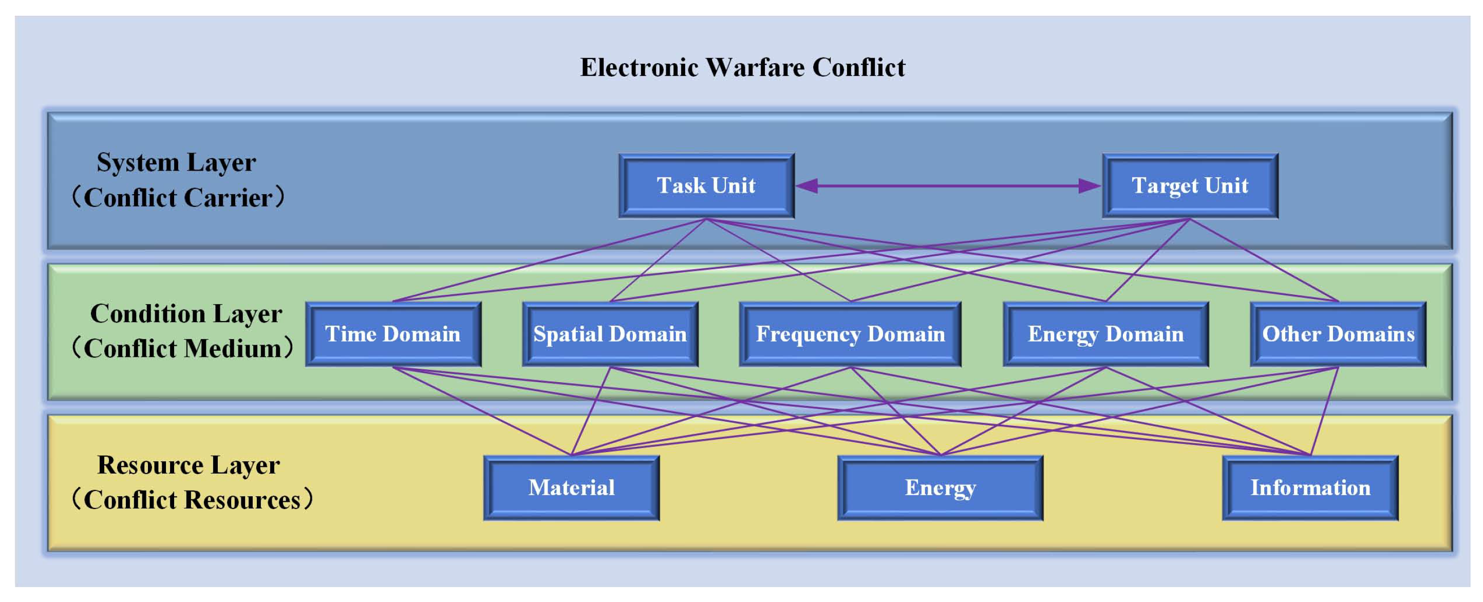
After the interaction of $R_{jk}$, the ${\mathsf{\Theta }}_j$ and ${\mathsf{\Gamma }}_k$ states of the system change, and the effective state $\eta$ of the system changes too, resulting in state conflicts, which are manifested as changes in resource requirements or functional states. Considering the conditions for the effectiveness of EW, system conflicts are reflected in time domain, airspace domain, frequency domain, energy domain and other conditional domains [10]. Conflicting resource needs are reflected in material, energy or information and so on. The hierarchical conflict structure corresponding to EW conflicts is shown in Figure 1.

2.3. State Mapping of EW Conflict Systems

EW conflict is a relationship that corresponds to the state between conflicting system units. The state of the EW conflict system unit refers to the state in which the EW system Unit is located. Since the EW unit system needs to meet certain conditions to achieve its function/purpose that is the media attribute, therefore the mapping relationship between the system and its conditions must be established first. According to the factor space theory [30,31], there are

$$f:U\to X\left(f\right)=\left\{a_1,a_2,\dots \right\}$$

(2)

where U is a unit system involved in the conflict system, f represents any conditional state of the system, $X\left(f\right)$ represents the conditional state space of the system, and $a_1,a_2,\dots$ is the characteristic attribute corresponding to each condition, which is represented by various indicators.

The basic premise of EW effectiveness evaluation is to analyze the change of the conditional characteristic attribute before and after the conflict. The specific conditional characteristic attributes are related not only to the related conflict unit system, but also to the mechanism of operation and the desired effect. The evaluation can be for either a specific conditional feature attribute or a comprehensive conditional feature attribute, depending on the purpose and requirements of the evaluation. Correspondingly, a condition may be a set of basic condition states or a synthesis of the basic condition state sets.

Specifically, in an EW conflict system, because of the openness of electromagnetic signal propagation, the receiver of target unit systems such as radar and communication receive useful signals as well as other signals, which may affect useful signals. Task unit system, in order to achieve the desired effect, that is, to effectively achieve interference, interference signals must be well received by the receiver in order to affect the detection, tracking, communication or other functions of the target. However, all receivers are designed for the received signals, that is, the receiver has the best reception performance for the received signals. Therefore, in an effort to make the interference signal affect the receiver effectively, the interference signal propagating to the receiver should have the basic condition to affect the jammed receiving system. This is the condition of effective interference and also the basic condition for the analysis of the conflict state of EW. At present, the basic conditions of effective interference mainly include time domain, space domain, frequency domain and energy domain. In addition to these conditional domains, there are other requirements such as polarization domain, interference style, etc., to achieve effective interference [32]. These relatively independent conditions are called basic conditions. The basic condition state of the system plays a decisive role in the control phase of the system state transition. Without accurate state information input, it is impossible to determine whether the next state transition control is to be performed. To do this, it is necessary to first set up the basic condition state set for EW conflicts.

Define 3.

EW Conflict Basic Conditions State Set.

In the course of system conflict of each unit in EW, given n independent conditions of validity of unit system U, the mapping relationship of conflict unit system on condition $e_j$ is $e_j:U\to X\left(e_j\right)\left(j=1,2,\dots ,n\right)$, which is called basic condition state and is abbreviated as e. The set of n basic condition states is denoted as $F=\left\{e_1,e_2,\dots ,e_n\right\}$, which is called the basic condition state set, or the basic set for short [31].

In fact, the requirements of conditions for EW conflict states are multidimensional, and to reduce the impact of correlation among dimensions on the evaluation results (e.g., frequency domain also has time domain limitations, energy domain conditions and airspace conditions also have correlations). A given condition is often a combination of basic conditions, that is, any set of conditional states can be represented as an extension of a finite basic condition state. The definition of extended conditional state set is given.

Define 4.

Extended Conditional State Set.

For any conditional state set $f=\left\{e_{\left(1\right)},e_{\left(2\right)},\dots ,e_{\left(k\right)}\right\}$, the extended conditional state is defined as [31]:

$$X\left(f\right)=X\left(e_{\left(1\right)}\right)\times X\left(e_{\left(2\right)}\right)\times \dots \times X\left(e_{\left(k\right)}\right)$$

(3)

For example: $e_1$ is time domain state, $X\left(e_1\right)=4s$; $e_2$ is frequency domain state, $X\left(e_2\right)=\left[8GHz,12GHz\right]s$; $e_3$ is energy domain state, $X\left(e_3\right)=100W$; $e_4$ is space state, $X\left(e_4\right)=5^{\circ }$. Based on all above basic condition states, a basic condition state of the EW unit system is determined. If $e_5$ is the radiation state of the transmitter, it is related to the preceding conditions, at which point the established state is the extended condition state of the EW unit system.

In the conflict system of EW, task unit and target unit are typically non-cooperative. The connotation of EW effectiveness evaluation is to quantitatively calculate and qualitatively analyze the states of task unit and its impact on the basis of information fusion between the two parties, and to form a process of judging and making decisions. This process is manifested by describing the state of the systems on both sides and determining the degree of threat and impact [5]. Therefore, the state of both the task unit and the target unit should be considered to clarify the operation of the state set between multiple unit systems.

Theorem 1.

Conditional State Set Operation

Set f as the EW Task Unit Conditional State Set, g as the EW Target Unit Conditional State Set, and the following rules of operation between f and g are established [31]:

$$\begin{array}{c}X\left(f\cap g\right)=X\left(g\cap f\right)\end{array}$$

(4)

$$\begin{array}{c}X\left(f\cup g\right)=X\left(g\cup f\right)\end{array}$$

(5)

$$\begin{array}{c}X\left(f\cup g\right)=\prod \left\{X\left(e_j\left|e_j\in F,e_j\in f\cup g\right.\right)\right\}\end{array}$$

(6)

$$\begin{array}{c}X\left(f\cap g\right)=\prod \left\{X\left(e_j\left|e_j\in F,e_j\in f\cap g\right.\right)\right\}\end{array}$$

(7)

$\mathsf{\Pi }$ represents the Descartes product space. If ${\mathsf{\Theta }}_j$ and ${\mathsf{\Gamma }}_k$ condition states are complete enough, the $X\left(f\right)$ combined with the condition States is represented as a full condition state of the EW conflict. Any two different states have different conditional state attribute values to distinguish them. Then, the EW conflict system can be described using the EW states of the full-condition dimension.

3. Modeling EW Conflict State Space

After describing the conflict unit system as a state, the entire EW conflict can be mapped to a state space as a state [33]. State transitions in space form state tracks. To this end, this section mainly solves the problem of state space establishment and state track description modeling. Specifically, firstly, the basic criteria and conflict state hypothesis of effectiveness analysis are established. Secondly, based on the measurability analysis of conditional state attributes, the measurable conditional state space for EW conflicts is constructed. Finally, the formal description of EW conditional state transition track is analyzed.

3.1. EW Effectiveness Analysis Criteria and Conflict State Assumptions

In the EW conflict system, the conflict states is measured by the degree of satisfaction of the document [1]. There are two possible fulfillment states for each conditional state attribute: fulfillment or dissatisfaction. Conditional state is a synthesis of conditional state attributes, which corresponds to three possible satisfaction states: fully satisfied, partially satisfied (limited to multiple conditional state attributes), or unsatisfied. System state is the synthesis of conditional state, and there should also be three possible states of satisfaction: fully satisfied, partially satisfied or unsatisfied. In this way, the conflict state of EW constitutes a sequence of satisfied states under different operational conditions of the system. Various state transitions of the system reflect the variation of satisfaction degree, which also reflects the different effectiveness state changes of the system. Therefore, the key to effectiveness analysis is the analysis of state transition.

According to the relationship between the front and back of the system state, the state of the EW system unit is divided into observation state, transition state and expected state. The observation state is the system state in the current operational situation. Direct measurement and reading can determine the observation state of your own system unit. The use of military intelligence and information can help determine the observation states of the target party’s system units. The transition state is the subsequent state of the adjustment of the observation state, which needs to be determined according to the change of the state attribute of the observation state condition. Expected state is the expected state of the system when the system meets the required target conditions. Usually, it is determined by system technology, performance, tasks and experience. The expected state is an ideal prediction of the future state from its own point of view, combined with the actual system. In the actual application process, due to various restrictions, the transition state often approaches the expected state, but it is difficult to achieve the expected state. The relationship between the observed state at the current moment, the possible transition state, and the expected state in the future reflects the course of the EW conflict. This process is also closely related to the effectiveness. On this basis, the following assumptions may be made.

Hypothesis 1.

The degree of state approximation can reflect the level of effectiveness.

In the process of EW effectiveness evaluation, the expected state is used as the reference for EW system effectiveness evaluation. When the transition state produced by the observation state transition approaches the expected state, the effectiveness of the system is better than that far away from the expected state. In this way, the best effectiveness of the system can be achieved by describing the actual situation of EW condition state attributes, choosing appropriate strategies (represented by various decisions) to control the state change, making the transition state of one’s own side move towards approaching the expected state, and the observation state of the target unit move away from the expected state.

Hypothesis 2.

The degree of state approximation can be divided into several levels, which correspond to each conditional state.

The purpose of the evaluation is to make decisions. In order to match the fuzziness of decision-making, in the process of EW effectiveness evaluation, it is helpful to assist EW decision-making and optimize the effectiveness by fuzzifying the approaching degree into superior and inferior levels. It is also helpful to analyze the condition states.

Hypothesis 3.

The conditional state feature attribute is monotonic.

The conditional state attribute has relatively fixed directional/targeting during the transition adjustment process, that is, the monotonic relationship between the expected value and the observed value. Specifically, before the expected value is reached, the larger the observed value is better, or the smaller the observed value will be better. It is important to note that monotonicity is relative to a particular characteristic attribute of a conditional state. The integration of multiple monotonicity needs to be considered separately.

3.2. Construction of Measurable Conditional State Space for EW Conflicts

For the EW conflict system, the dynamic characteristics of the system need to be described according to the conditional state feature attributes. The vector formed by the conditional state feature attributes is called the conditional state vector, and the multidimensional conditional state space formed by the conflict conditions is called the EW conflict state space.

Define 5.

EW Conflict Conditional State Space.

Set $X\left(f\right)$ is the state space defined on the unit system U, and $X\left(f\right)\subset R^n$, and there is a set $\left\{a_1,a_2,\dots ,a_n\right\}$ of n-dimensional feature attributes defined on $X\left(f\right)$. When the dimensions in $X\left(f\right)$ represent the conditional state of a conflict, $X\left(f\right)$ is called the EW conflict conditional state space [34].

In the state space, the unit system U corresponds to the conditional state space. Conditional state feature attributes are the key variables to establish the observational state equation and the transition state equation. They are a set of independent and complete variables that can describe the dynamic characteristics of the system. To ensure the feasibility of effectiveness evaluation, conditional state feature attributes must be descriptive, essentially ensuring that each conditional state feature attribute is measurable in the unit system.

Proposition 1.

Conditional state attributes are measurable.

If the characteristic attribute of a conditional state can be obtained directly or indirectly from the outside by some means, it is called measurable.

Conditional state attributes can be measured not only to judge whether the output state of the system meets expectations, but also directly determine whether the system condition state is measurable.

Define 6.

Measurable Conditional State.

Let $\left(U,A\right)$ be the measurable space on unit system U, and A be the set of all measurable attributes of the system. For conditional state mapping $e:U\to X\left(e\right)$, if $\left[a_i\right]=e^{-1}\left(a_i\right)=\left\{u\in U\left|e\left(u\right)=a_i\right.\right\}\in A$ exists for any conditional state attribute $a_i\in X\left(e\right)$, e is called a measurable conditional state [31].

Many states in the description of EW conflict state are inevitably based on the synthesis of basic condition states, that is, extended condition states. Quantitative effectiveness analysis can only be performed better if all extended condition states are measurable.

Proposition 2.

Extended State Measurable

For the basic condition state set $F=\left\{e_1,e_2,\dots ,e_n\right\}$, if any $e_j\in F\left(j=1,2,3,\dots ,n\right)$ is measurable, the extended condition state f is measurable.

Define 7.

Measurable Conditional State Space.

Given the conditional state space $G=\left(\left(U,A\right),X_F,P\right)$ on unit system U, if every basic conditional state in G is measurable, then G is called measurable conditional state space. $X_F$ is the extended conditional state set and $P=F_{\xi }\left(x\right)\left(\xi \le x\right)$ is the state probability distribution function of $\xi$ [31].

Conditional state space measurable is the basis for solving non-cooperative conflicts in EW in complex electromagnetic environment. On this basis, controlling state transition can also control the degree and direction of conflicts. In state space, continuous state control is represented as a state track generated by states over time series.

3.3. Generation of EW Conditional State Transition Track

The set of points that meet a certain condition is called the locus of the point that meets that condition. Correspondingly, the set of states that meet a certain condition is called the state track that satisfies the condition. Suppose the expected state of the EW system unit is $\widehat{X}$ and the observed state is $X_0$. $\widehat{X}$ is the system state when the system meets the required target conditions; $X_0$ is the system state under the current operational conditions. $X^{-}$ is the worst-condition state, constituting the lower bound of the state. When the value of the conditional state attribute is lower than that of the conditional state attribute in $X^{-}$, the conditional state attribute of the system unit participating in the conflict is no longer available. $X^{+}$ is the ideal state conditional attribute value, which constitutes the upper bound of the state. When the conditional state attribute value approaches the conditional state attribute value in $X^{+}$, the system units participating in the conflict approach the ideal state. In practice, the expected state and the observed state are between the ideal state and the worst state. Conflict state transition track is formed when the system state transits between ideal state and worst state.

Define 8.

Valid Conditional State Track.

Set $X_{\left(i\right)}^{*}\left(f\right)\subset X\left(f\right)$, $f_i\in f$, given the constant $k_{i1}<k_{i2}$. $\forall a\in X_{\left(i\right)}^{*}\left(f\right)$, according to the EW validity condition, if $f_i\left(a\right)\le k_{i2}$ or $f_i\left(a\right)\ge k_{i1}$, $k_{i1}\le f_i\left(a\right)\le k_{i2}$ is satisfied, the conditional state is valid, then $X_{\left(i\right)}^{*}\left(f\right)$ is called the valid conditional state track [34].

The valid conditional state trajectories $X_{\left(i\right)}^{*}\left(f\right)$ are a valid subset of the conditional state attributes that can characterize the characteristics of the system’s transient response. For the expected condition state attribute, the condition state that satisfies the conflict state track is called the valid expected state track, otherwise it is called the invalid expected state track. For the Observation/Transition State Conditional Feature attribute, the condition state that satisfies the conflict state track is called the valid observation/transition state track, otherwise it is called the invalid observation/transition state track.

Define 9.

Complete Conditional State Track.

If $X^{*}\left(f\right)=\bigcap _i{X}_{\left(i\right)}^{*}\left(f\right)$, $X^{*}\left(f\right)$ is the intersection of $X_{\left(i\right)}^{*}\left(f\right)$ determined by all functions in f, $X^{*}\left(f\right)$ is the subset of $X\left(f\right)$ that can meet the requirements of each conditional state, called the complete conditional state track [34].

Define 10.

Under-Complete Conditional State Track.

If $\exists k\le i$, $X^{*}\left(f\right)=\bigcap _k{X}_{\left(k\right)}^{*}\left(f\right)$, $X^{*}\left(f\right)$ is the intersection of determined by some functions in f. $X^{*}\left(f\right)$ is a subset of $X\left(f\right)$ that satisfies some conditional state requirements, called the under-complete conditional state track.

Proposition 3.

Conflict State non-transferability

If $\forall k\le i$, $\bigcap _k{X}_{\left(k\right)}^{*}\left(f\right)=\varphi$, there is no intersection of $X_{\left(k\right)}^{*}\left(f\right)$ determined by the function in f, that is, there is no conditional state track, then the conflict state is not transferable. In the process of EW operation, a large number of conditional state tracks belong to the undercomplete state.

Define 11.

Conditional State Track Surface.

If $M_i$ is the set of all valid points corresponding to $\forall a\in X_{\left(i\right)}^{*}\left(f\right)$ and $f_i\left(a\right)=k_i$, then $M_i$ is called the conflict state track surface and $M={\displaystyle \bigcap _i}{M}_i$ is the complete conflict state track surface [34].

In state space, state tracks represent the paths described by state vector endpoints over time. The state track corresponds to the state of the system at different times and under different conditions. Once the state track is established in a certain period of time, the change process of the system in that time can also be determined. Therefore, the description method of the conflict state track is an effective way to study the dynamic change of the effectiveness of the EW conflict system in conflict space.

Assume that ${\widehat{X}}_{\alpha }$ and ${\widehat{X}}_{\beta }$ are the expected states of ${\mathsf{\Theta }}_j$ and ${\mathsf{\Gamma }}_k$, respectively, $X_{\alpha 0}$ and $X_{\beta 0}$ are the dynamic observation states of ${\mathsf{\Theta }}_j$ and ${\mathsf{\Gamma }}_k$, respectively, $p\left(\right)$ is a monotonically increasing polynomial function, and $R_{\alpha \beta }$ is the conflict relationship between the two unit systems. $R_{\alpha \beta }$, ${\mathsf{\Theta }}_j$ and ${\mathsf{\Gamma }}_k$ belong to the direct confrontation state, then there are:

$$X_{\alpha 0}\propto p^{-1}\left(X_{\beta 0}\right)$$

(8)

The first-order partial derivatives of $X_{\alpha 0}$ and $X_{\beta 0}$ about time will stabilize after a certain time $t\to \mathrm{T}$, and their ratio will converge to the constant [28]. This relationship is expressed as follows:

$$\left(X_{\alpha 0}\left(t\right),X_{\beta 0}\left(t\right)\right)\in \left\{〈A,U〉\left|\underset{t\to \mathrm{T}}{lim}\left(\frac{\partial X_{\alpha 0}/\phantom{\partial X_{\alpha 0}\partial t}\partial t}{\partial X_{\beta 0}/\phantom{\partial X_{\beta 0}\partial t}\partial t}\right)=const<0\right.\right\}$$

(9)

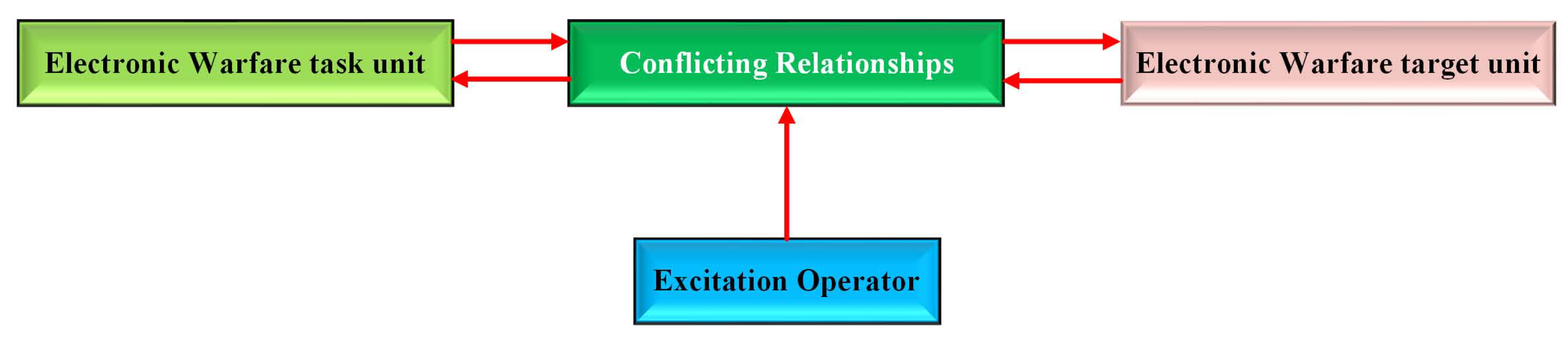
The physical meaning of partial derivation represents the direction and intensity of state changes between task units and target units over time. The change of state essentially refers to the change of conflict relationship between EW conflict systems. Specifically, it refers to the change of condition state attributes under certain external incentive conditions. To this end, the description of the system (1) is modified, and the excitation operator ∇ (represented by decision implementation) is defined to change the state of interrelationship, which is described as:

$$U=\left\{\left\{U_i\left|i\in I\right.\right\},\left\{\left({\nabla }_{jk},R_{jk}\right)\left|j\in I,k\in I,and,J\ne K\right.\right\}\right\}$$

(10)

The basic system relationships form as shown in Figure 2:

Under the relationship $R_{\alpha \beta }$, changes in ${\nabla }_{\alpha \beta }$ make $X_{\alpha 0}$ correspond to two states: expected state ${\widehat{X}}_{\alpha }$ and transition state $X_{\alpha 0}^{*}$. By analyzing the degree of transition state $X_{\alpha 0}^{*}$ approaching ${\widehat{X}}_{\alpha }$, the degree of conditional state satisfaction under the restrictions of EW system resources and conditions can be obtained. Under the influence of excitation ${\nabla }_{\alpha \beta }$, the expected state may change and the observed state may shift. The change of conflict state track reflects the change of conflict relationship as well as the change of degree that meets the requirements, that is, the dynamic change of EW effectiveness.

4. Dynamic Transfer Analysis of EW Conflict State Based on Markov Process

According to the previous analysis, the dynamic change of EW effectiveness depends on the analysis of conflict state transition change, and the modeling of the transition process becomes the key to the study. This section focuses on the modeling of conflict state transition processes. Specifically, first, by analyzing the uncertainty of EW conflict, the EW conflict state transition is described as a Markov random process. Secondly, the relevant properties of Markov process dynamic transfer in the conflict state of EW are analyzed. Finally, the transition state probability description of the transfer process is analyzed.

4.1. EW Conflict State Markov Random Processes

The traditional methods of EW effectiveness evaluation are usually linear weighted overlay of each subsystem. However, in the process of practice and research, it is found that the EW effectiveness is obviously inadequate expressed by a simple combination of various indicators (such as linear weighting), but the interaction between the indicators, which will make the evaluation results quite different. Especially for complex systems, each index has a close correlation, and it is difficult to guarantee the independence of each other. The additive or quasi-additive function cannot be used to represent the overall performance. It is more a multi-condition state relationship. Here, we describe the effectiveness characteristics of the EW system by using the process parameters of the EW conflict state changing from the observation state to the expected state, and the system effectiveness evaluation index is described by the conditional state attribute.

The system changes from an observation state to a transition state, which constitutes a transition process. A unit system can be affected in different ways over a period of time, either actively or passively. Due to the multivariate and random distribution of EW system conditional state attributes, and the possible effects of non-cooperative difficulties in accurate measurement, the EW system state has random uncertainty directly. In addition, the system state of the EW task unit is closely related to the environment in which the system is located, especially the electromagnetic environment, which is complex and variable, and is also an important reason for the uncertainty of the state of the EW system. Therefore, the process of changing the conflict state of EW can be described as a random process [35].

Define 12.

EW Conflict State Random Process.

Given EW conflict state space $G=\left(\left(U,A\right),X_F,P\right)$, $X_F$ is the attribute set of conditional state F. Set a time parameter set T. For $\forall t\in T$, at least one random state variable $f_t\left(X\right)$ is defined in G, then set $\left\{f_t\left(X\right)\left|t\in T\right.\right\}$ is called EW conflict state random process [31].

From the point of view of system observation state, the conflict system of EW consists of at least two subsystems conflicting and interacting with each other, which is mapped to two opposing and related conflict states. From the operation process, EW is a multi-step and dynamic process in which the target unit and task unit continuously transfer their observation state to approach the expected state. The transfer process reflects the decision-making adjustment process of both sides based on the effect. The whole process is considered to consist of cascades of several sub-processes called “observation state-transition state-expected state”. This sub-process contains the basic characteristics of EW conflict and is the basic object of study. Considering that the expected state is only related to the observation state of both sides, but not to the state before the observation state, and the transition between states has some uncertainty or probability, the randomness is introduced into the EW effectiveness state space. In the space, a conflict state transition model between the observed state and the transition state of the EW system is established.

The transition state of an EW system is only related to the observed state and the excitation. It is a random transition process with no aftereffect conflict state. Therefore, the Markov transformation process of EW conflict states can be used as a model description method.

Define 13.

EW Conflict State Markov Process.

Suppose that $\left\{f_t\left(X\right)\left|t\in T\right.\right\}$ is a random process of state transition for a unit system defined on the measurable space $G=\left(\left(U,A\right),X_F,P\right)$ of an EW conflict state. If there has $P\left(a_{i+1}\left|a_{i-1}{a}_i\right.\right)=P\left(a_{i+1}\left|a_i\right.\right)$ for any corresponding conditional state attribute $a_i\in X\left(t_i\right)$ at any time $t_i$, then $\left\{f_t\left(X\right)\left|t\in T\right.\right\}$ is the Markov process for EW conflict state [31].

In the Markov process, according to the Chapman-Kolmogorov Equations, if the observed state and the state transition probability matrix of the EW conflict system are known, after a period of k transfers, the system exists in a limit transfer state of a certain limit probability. Depending on how close this limit transfer state approximates the expected state after this period of time, it can be used to support state transition decisions. Therefore, when the observed state is known, the state transition track can be controlled by controlling the state transition matrix, so that the conflict states between the EW task unit and the target unit can be related through the state transition probability matrix. By introducing Markov chains into the state space, the dynamic control of the state transition probability matrix is realized, which also implements the dynamic control of the system state.

4.2. Dynamic Transition of Markov Process in EW Conflict State

4.2.1. Multi-step Markov Transfer of Discrete Conflict States

The transition of state attributes of EW conflict conditions can be expressed as a matrix. This matrix is not only a kinematic representation of the conflict state, but also a behavioral representation of the conflict decision-making. For this reason, it is clear that the state transition matrix is the first step to study the conflict state Markov process.

Define 14.

State Transition Probability Matrix [31].

In the EW conflict state space, observation state $X_0$, transition state $X_0^{*}$ and expected state $\widehat{X}$ are all comprehensive representations of conditional states. If each state is made up of n conditional state $f_1,f_2,\dots ,f_n$ by the Cartesian product. There are $m_i$ conditional state attributes for conditional state $f_i\left(i=1,2,\dots ,n\right)$, and the conditional state attributes of $f_i$ is denoted as $X\left(f_i\right)=\left(a_1^{\left(i\right)},a_2^{\left(i\right)},\dots ,a_{m_i}^{\left(i\right)}\right)$. Each conditional state attribute $a_{m_i}^{\left(i\right)}$ has a total of $n_i$ attribute states, denoted as $a_{m_i}^{\left(i\right)}=\left(b_{m_{i}1}^{\left(i\right)},b_{m_{i}2}^{\left(i\right)},\dots ,b_{m_i{n}_i}^{\left(i\right)}\right)$.The conditional state attribute $a_{m_i}^{\left(i\right)}$ transition probability matrix is:

$$P_{m_i}^{\left(i\right)}=\left[\begin{array}{cccc}{P}_{m_{i}11}^{\left(i\right)}& P_{m_{i}12}^{\left(i\right)}& \dots & P_{m_{i}1n_i}^{\left(i\right)}\\ P_{m_{i}21}^{\left(i\right)}& P_{m_{i}22}^{\left(i\right)}& \dots & P_{m_{i}2n_i}^{\left(i\right)}\\ \dots & \dots & \ddots & ⋮\\ P_{m_i{n}_{i}1}^{\left(i\right)}& P_{m_i{n}_{i}2}^{\left(i\right)}& \dots & P_{m_i{n}_i{n}_i}^{\left(i\right)}\end{array}\right]$$

(11)

In the formula, $P_{m_{i}mn}^{\left(i\right)}\left(m,n=1,2,3,\dots ,n_i\right)$ represents the probability that the attribute state will transfer from $b_{m_{i}m}^{\left(i\right)}$ to $b_{m_{i}n}^{\left(i\right)}$, obviously $P_{m_{i}mn}^{\left(i\right)}\ge 0$, and:

$$\sum _{n=1}^{n_i}{P}_{m_{i}mn}^{\left(i\right)}=1$$

(12)

If the EW conflict system starts from any observed state $X_m\left(X_m\in X\left(t_m\right)\right)$ at time $t\left(t=0,1,2,\dots \right)$ and transfers to a state $X_n\left(X_n\in X\left(t_m\right)\right)$ in state space $X\left(t_m\right)$ at time $t+k\left(k=1,2,\dots \right)$, then any conditional state attribute transfer probability $P_{m_{i}mn}^{\left(i\right)}\left(t,t+k\right)$ must be satisfied:

$$\left\{\begin{array}{c}{P}_{m_{i}mn}^{\left(i\right)}\left(t,t+k\right)\ge 0\hfill \\ {\displaystyle \sum _{\underset{n}{X}\in X\left(t_m\right)}}{P}_{m_{i}mn}^{\left(i\right)}\left(t,t+k\right)=1\hfill \end{array}\right.$$

(13)

The matrix consisting of state transition probability $P_{m_{i}mn}^{\left(i\right)}\left(t,t+k\right)$ is the k-step state transition probability matrix of conditional state attribute $a_{m_i}^{\left(i\right)}$, denoted as $P_{m_i}^{\left(i\right)}\left(t,t+k\right)$ and abbreviated as $P_{m_i}^{\left(i\right)}\left(k\right)$. When $k=1$, $P_{m_i}^{\left(i\right)}\left(1\right)$ is called the single-step state transition probability matrix. In the state transition probability matrix, the sum of the elements in each row is equal to 1.

If the conditional state attribute has finite attribute state $a_{m_i}^{\left(i\right)}=\left(b_{m_{i}1}^{\left(i\right)},b_{m_{i}2}^{\left(i\right)},\dots ,b_{m_i{N}_i}^{\left(i\right)}\right)$ in the process of EW conflict, the single-step state transition probability $P_{m_i}^{\left(i\right)}\left(1\right)$ can form a finite N-order matrix, denoted as $P_{m_i}^{\left(i\right)}$:

$$P_{m_i}^{\left(i\right)}=P_{m_i}^{\left(i\right)}\left(1\right)=\left[\begin{array}{cccc}{P}_{m_{i}11}^{\left(i\right)}& P_{m_{i}12}^{\left(i\right)}& \dots & P_{m_{i}1N}^{\left(i\right)}\\ P_{m_{i}21}^{\left(i\right)}& P_{m_{i}22}^{\left(i\right)}& \dots & P_{m_{i}2N}^{\left(i\right)}\\ ⋮& ⋮& \ddots & ⋮\\ P_{m_{i}N1}^{\left(i\right)}& P_{m_{i}N2}^{\left(i\right)}& \dots & P_{m_{i}NN}^{\left(i\right)}\end{array}\right]$$

(14)

Considering the scalability and unknown nature of the conflict conditions, if the conditional state attribute has an infinite state $a_{m_i}^{\left(i\right)}=\left(b_{m_{i}1}^{\left(i\right)},b_{m_{i}2}^{\left(i\right)},\dots \right)$, then the state transition probability matrix $P_{m_i}^{\left(i\right)}$ is:

$$P_{m_i}^{\left(i\right)}=\left[\begin{array}{ccc}{P}_{m_{i}11}^{\left(i\right)}& P_{m_{i}12}^{\left(i\right)}& \dots \\ P_{m_{i}21}^{\left(i\right)}& P_{m_{i}22}^{\left(i\right)}& \dots \\ ⋮& ⋮& ⋮\end{array}\right]$$

(15)

Similarly, all elements of matrix $P_{m_i}^{\left(i\right)}$ are nonnegative, and the sum of each row of elements is equal to 1.

4.2.2. Continuous Time Transfer of Discrete Conflict State

In the analysis of the state transition process, it is necessary to know the probability density $p_{m_{i}mn}^{\left(i\right)}$ corresponding to the state transition probability $P_{m_{i}mn}^{\left(i\right)}$ [36]:

$$p_{m_{i}mn}^{\left(i\right)}=\underset{\mathsf{\Delta }t\to 0}{lim}\frac{P_{m_{i}mn}^{\left(i\right)}\left(\mathsf{\Delta }t\right)}{\mathsf{\Delta }t}$$

(16)

In the formula, $P_{m_{i}mn}^{\left(i\right)}\left(\mathsf{\Delta }t\right)$ represents the probability that the system will transfer from attribute state $b_{m_{i}m}^{\left(i\right)}$ to state $b_{m_{i}n}^{\left(i\right)}$ at time T after time $\mathsf{\Delta }t$.

When all probability densities $p_{m_{i}mn}^{\left(i\right)}$ are independent of time T, this Markov process is called homogeneous, otherwise it is nonhomogeneous. In fact, the transfer probability density changes with the change of the transfer control strategy of the system’s own state and the conflicting unit system’s countermeasure strategy. This change is consistent with the nature of non-cooperative conflict in EW and is a direct reflection of the related attributes of EW conflict state. Based on the analysis of state transition probability matrix, a system state transition model describing a one-step sub-process of “observation state-transition state-expected state” in the course of EW conflict is established. Persistently, multi-step state transition enables dynamic analysis of the entire process of EW conflict states.

Proposition 4.

State Reciprocity [31]

The conditional state corresponding to observation state X is $\left(f_1,f_2,\dots f_n\right)$. $f_i$ corresponds to the conditional state property $\left(a_1\left(X\right),a_2\left(X\right),\dots ,a_{m_i}\left(X\right)\right)$. The attribute state corresponding to conditional state attribute $a_{m_i}\left(X\right)$ is $\left(b_{m_{i}1}\left(X\right),b_{m_{i}2}\left(X\right),\dots ,b_{m_i{n}_i}\left(X\right)\right)$. The conditional state attribute $a_{m_i}\left(X\right)$ of state $X^{\prime }$ corresponds to the property state

$\left(b_{m_{i}1}\left(X^{\prime }\right),b_{m_{i}2}\left(X^{\prime }\right),\dots ,b_{m_i{n}_i}\left(X^{\prime }\right)\right)$. During the state transition process, due to the uncertainty of the effectiveness state, the attribute states of any conditional state attribute $a_{m_i}\left(X\right)$ of state X and state $X^{\prime }$ can be exchanged with each other over time, that is $b_{m_{i}m}\left(X\right)\leftrightarrow b_{m_{i}n}\left(X^{\prime }\right)$.

The reciprocity of States reflects to some extent the uncertainty and unknown in the decision-making process of operations.

The state transition depends on the excitation operator. Incentives are divided into positive incentives and negative constraints according to their effect. The main purpose of positive motivation is to maintain or enhance the relationship under the current state conflict. Negative constraints mainly weaken or reduce conflict relationships. Under different excitation conditions, the system effectiveness changes differently.

Define 15.

State Transition Probability [36].

Transfer $\left(X_0\to \widehat{X}\right)$ from the observed state to the expected state is a composite result of the transfer of attribute state $b_{m_{i}m}\left(X_0\right)\to b_{m_{i}m}\left(\widehat{X}\right)\left(m=1,2,\dots ,n_i\right)$ corresponding to conditional state attribute $a_{m_i}\left(X\right)$. Assuming that each conditional state attribute $a_1\left(X\right),a_2\left(X\right),\dots ,a_{m_i}\left(X\right)$ is independent of each other, the probability of conditional state attribute $a_{m_i}\left(X\right)$ transition from state $X_0$ to state $\widehat{X}$ is:

$$P_{X_0\widehat{X}}=P_{X_0\widehat{X}}^{\left(1\right)}{P}_{X_0\widehat{X}}^{\left(2\right)}\dots P_{X_0\widehat{X}}^{\left(n_i\right)}$$

(17)

In the formula above, $P_{X_0\widehat{X}}^{\left(m\right)}\left(m=1,2,\dots ,n_i\right)$ refers to the probability that the $m_i$-th conditional state attribute of state $X_0$ corresponds to the property corresponding to the m-th state attribute transferred to state $\widehat{X}$, which can be found in the attribute transfer probability matrix or based on the corresponding probability density.

4.2.3. Chapman-Kolmogorov Equations of EW Conflict State

In the Markov transition process of the EW conflict state, for any positive integer k, l, if there are:

$$P_{mn}\left(k+l\right)=\sum _{{\widehat{X}}_s\in X\left(t_m\right)}{P}_{ms}\left(k\right)P_{sn}\left(l\right),{\widehat{X}}_s\in X\left(t_i\right)$$

(18)

The above equation is called Chapman-Kolmogorov Equation(C-K equation) of EW conflict state [37].

According to the C-K equation, the process of transition from observed state $X_m$ to expected state ${\widehat{X}}_n$ through step $k+l$ can be decomposed into the union of processes from state $X_m$ to state ${\widehat{X}}_s\left({\widehat{X}}_s\in X\left(t_m\right)\right)$ through step k and from ${\widehat{X}}_s$ to state ${\widehat{X}}_n$ through step l. The process is independent for different intermediate expected states ${\widehat{X}}_s$.

The matrix of the C-K equation is expressed as $P\left(k+l\right)=P\left(k\right)P\left(l\right)$. For $k=l=1$, there are:

$$P\left(2\right)=P\left(1\right)P\left(1\right)=PP=P^2$$

(19)

Generally, $P\left(k\right)=P^k,k=1,2,\dots$ holds. This indicates that the k-step state transition probability matrix of the state Markov process is equal to the product of k single-step transition probability matrices, so the k-step state transition probability can be derived from the single-step state transition probability. In subsequent studies, we will focus on the probability of one-step state transition.

4.3. Transition State Probability Model

During the whole process of conflict analysis of EW, the observation state is mainly based on the use of EW and data collection, which is relatively easy to obtain. From the perspective of task unit system, the expected state is based on the expected state representation of the decision strategy itself; from the perspective of target unit system, it is based on the observed state of the target unit system and the state prediction of the decision strategy; and the transition state is the possible state transition in the decision implementation process. All three states have some uncertainty. This section gives a description of the probability of transition state.

In Conflict State Markov process $\left\{f_t\left(X\right)\left|t\in T\right.\right\}$, the conditional state property is $a_i\left(a_i\in X\left(t_i\right)\right)$. The probability of observing state $X\left(t_0\right)$ at the initial moment is:

$$P\left\{X\left(t_0=j\right)\right\}=P_j,a_j\in X\left(t_i\right)$$

(20)

The above formula, called the observed state probability of the Conflict State Markov process, is recorded as:

$$P=P\left(0\right)=\left(P_1,P_2,\dots ,P_j,\dots \right),a_j\in X\left(t_i\right)$$

(21)

The state probability of transition state $X\left(t_m\right)$ at time m is recorded as:

$$P\left\{X\left(t_m=j\right)\right\}=P_j,a_j\in X\left(t_i\right)$$

(22)

The above formula is called the transition state probability of the conflict state Markov process at time m and is written down as:

$$P\left(m\right)=\left(P_1\left(m\right),P_2\left(m\right),\dots ,P_j\left(m\right),\dots \right),a_j\in X\left(t_j\right)$$

(23)

In particular, the state probability distribution at time $m=0$ is the observed state probability distribution, which can be recorded as:

$$P\left\{X\left(t_0=j\right)\right\}=P_j=P_j\left(0\right),a_j\in X\left(t_i\right)$$

(24)

The transition state probability at time m satisfies the following conditions:

$$\begin{array}{c}{P}_j\left(m\right)\ge 0\end{array}$$

(25)

$$\begin{array}{c}\sum _{a_j\in X\left(t_i\right)}{P}_j\left(m\right)=1\end{array}$$

(26)

$$\begin{array}{c}{a}_j\in X\left(t_i\right),m=0,1,2,\dots \end{array}$$

(27)

If the probability $P_j\left(m\right)\left(a_j\in X\left(t_i\right)\right)$ of time m and the probability $P_{ij}\left(a_i,a_j\in X\left(t_i\right)\right)$ of one-step state transition are known, the probability of time $m+1$ is as follows:

$$P_j\left(m+1\right)=\sum _{a_i\in X\left(t_i\right)}{P}_i\left(m\right)P_{ij},a_j\in X\left(t_i\right),m\ge 0$$

(28)

If observed state probability $p_j\left(a_j\in X\left(t_i\right)\right)\left(j=1,2,\dots \right)$ and step m state transition probability $P_{ij}\left(m\right)\left(a_i,a_j\in X\left(t_i\right),m\ge 1\right)$ are known, then the probability distribution at time m is:

$$P_j\left(m+1\right)=\sum _{a_i\in X\left(t_i\right)}{P}_i{P}_{ij}\left(m\right),a_j\in X\left(t_i\right),m\ge 1$$

(29)

If the state-space condition attribute of the conflict process is $a_i\left(a_i\in X\left(t_i\right)\right),i=1,2,\dots N$. $P\left(1\right)$ is a one-step state transfer probability matrix, then the above expression can be expressed as:

$$\left(P_1\left(m\right),P_2\left(m\right),\dots ,P_N\left(m\right)\right)=\left(P_1,P_2,\dots ,P_N\right)P{\left(1\right)}^m,m\ge 1$$

(30)

Denoted by:

$$\begin{array}{c}P=P\left(0\right)=\left(P_1,P_2,\dots ,P_N\right)\end{array}$$

(31)

$$\begin{array}{c}P\left(m\right)=\left(P_1\left(m\right),P_2\left(m\right),\dots ,P_N\left(m\right)\right)\end{array}$$

(32)

Then the above formula can be expressed as:

$$P\left(m\right)=PP{\left(1\right)}^m$$

(33)

The transition state corresponding to the initial observation state is:

$$X\left(t_m\right)=X\left(t_0\right)P\left(m\right)$$

(34)

5. EW Effectiveness Evaluation Based on Markov Transfer Approximation Analysis

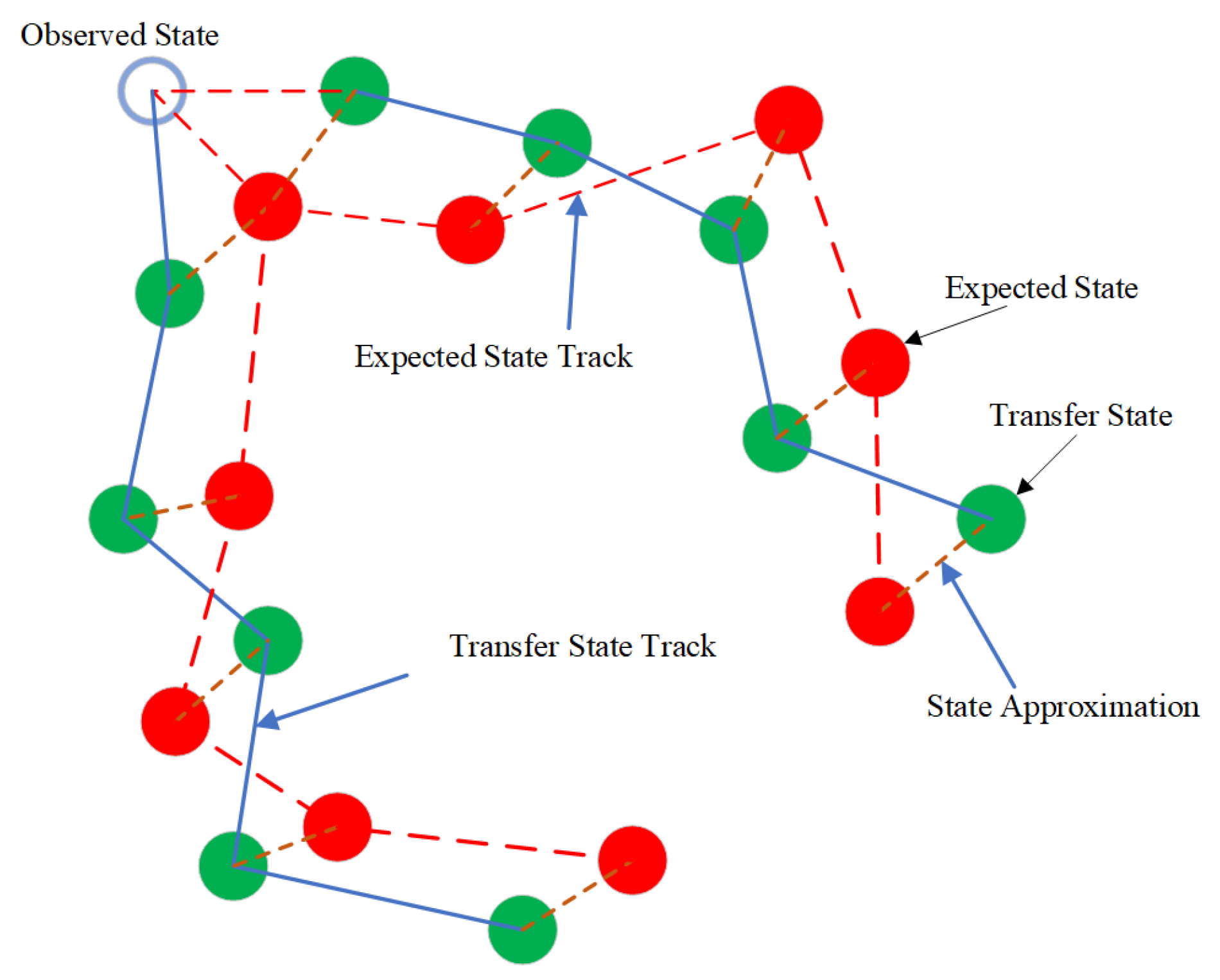
EW state conflict states are based on measurable of system state. Conflict models are used in theory, device experimentation, or practice to understand the state of an EW system. An effective method is to consider the degree of state correlation under the influence of conflicts and interactions. This section mainly evaluates the EW effectiveness based on the approximation between the transition state and the expected state.The specific association process is shown in the Figure 3.

5.1. Approximation of EW Conflict States

According to the previous analysis, the description from each conditional state is the unit system state matrix, the space constructed is the EW conflict state space, the expected state corresponds to the expected state matrix, and the observed state corresponds to the observed state matrix. According to the literature [1], the effectiveness of EW is related to the approximation of the transition state matrix and the expected state matrix to achieve specific requirements in the case of mission unit operations, and also to the approximation of the transition state matrix and the expected state matrix in the case of target unit operations. Generally speaking, the EW effectiveness should reflect the proximity and correlation of the transition state matrix and the expected state matrix of the task unit system and the target unit system. Gray correlation analysis is a method to analyze and determine the degree of influence or contribution of factors to the main behavior of the system by using gray correlation degree. The basic idea is to distinguish the degree of correlation among the multifactor in the system by comparing the similarity of the shape of the set of system statistical sequence curves [38,39].

Step 1.

Establish the original conflict state sequence based on the observed data.

In the EW state conflict system, each state is described by a state sequence, assuming that $X_{\alpha j}$ is the observation state sequence of the EW task unit. Since the state sequence is based on EW conditional validity analysis, it is assumed that conditional state $f_i$ has $m_i$ independent conditional state attributes, and the corresponding observation state sequence $X_{\alpha j}\left(f_i\right)$ is as follows:

$$X_{\alpha j}\left(f_i\right)=\left(a_1^{\left(i\right)},a_2^{\left(i\right)},\dots a_{m_i}^{\left(i\right)}\right)$$

(35)

Conditional state attribute $a_{m_i}^{\left(i\right)}$ can only be in one attribute state $b_{m_i}^{\left(i\right)}$ at a certain time, so

$$X_{\alpha j}\left(f_i\right)=\left(a_1^{\left(i\right)},a_2^{\left(i\right)},\dots a_{m_i}^{\left(i\right)}\right)=\left(b_1^{\left(i\right)},b_2^{\left(i\right)},\dots b_{m_i}^{\left(i\right)}\right)$$

(36)

For the convenience of subsequent analysis, attribute state $b_{m_i}^{\left(i\right)}$ is directly represented by $a_{m_i}^{\left(i\right)}$.

Step 2.

Constructing the boundary state sequence.

Considering that each conditional state has its own boundary, the sequence of upper and lower bounded States is constructed based on the attribute characteristics of each conditional state. The supremum state sequence of EW task unit:

$$X_{\alpha }^{+}\left(f_i\right)=\left(a_1^{\left(i\right)+},a_2^{\left(i\right)+},\dots a_{m_i}^{\left(i\right)+}\right)$$

(37)

The infimum state sequence of EW task unit:

$$X_{\alpha }^{-}\left(f_i\right)=\left(a_1^{\left(i\right)-},a_2^{\left(i\right)-},\dots a_{m_i}^{\left(i\right)-}\right)$$

(38)

Step 3.

Establishing the sequence of expected conflict states.

Based on task requirements and capability states, assume that ${\widehat{X}}_{\alpha }$ is the system expected state sequence, and for conditional state $f_i$ corresponds to different expected state sequence ${\widehat{X}}_{\alpha }\left(f_i\right)$:

$${\widehat{X}}_{\alpha }\left(f_i\right)=\left({\widehat{a}}_1^{\left(i\right)},{\widehat{a}}_2^{\left(i\right)},\dots {\widehat{a}}_{m_i}^{\left(i\right)}\right)$$

(39)

Obviously, for $\forall m\left(m=1,2,3,\dots ,m_i\right)$, there are:

$$\left\{\begin{array}{c}{a}_m^{\left(i\right)}\in \left[a_m^{\left(i\right)-},a_m^{\left(i\right)+}\right]\hfill \\ {\widehat{a}}_m^{\left(i\right)}\in \left[a_m^{\left(i\right)-},a_m^{\left(i\right)+}\right]\hfill \end{array}\right.$$

(40)

and for $\exists \epsilon \ge 0$, formula $\left|a_m^{\left(i\right)}-{\widehat{a}}_m^{\left(i\right)}\right|\le \epsilon$ holds.

Step 4.

Conditional State Attribute Transition Probability Matrix.

Conditional state attributes are transferred in different task requirements and capability states. Assume that the attribute state transition probability matrix corresponding to the conditional state attribute $a_m^{\left(i\right)}$ of conditional state $f_i$ is:

$$P_m^{\left(i\right)}=\left[\begin{array}{cccc}{P}_{m11}^{\left(i\right)}& P_{m12}^{\left(i\right)}& \dots & P_{m1n_i}^{\left(i\right)}\\ P_{m21}^{\left(i\right)}& P_{m22}^{\left(i\right)}& \dots & P_{m2n_i}^{\left(i\right)}\\ \dots & \dots & \ddots & ⋮\\ P_{m{n}_{i}1}^{\left(i\right)}& P_{m{n}_{i}2}^{\left(i\right)}& \dots & P_{m{n}_i{n}_i}^{\left(i\right)}\end{array}\right]$$

(41)

Step 5.

System state hierarchy and corresponding relationship of conditional state attributes

The state of each system will be different with the change of task and the uncertainty of battlefield situation. Assume that system task state $X_{\alpha j}$ corresponds to a state level of $L_j$. Each state has n conditional state $f_1,f_2,\dots ,f_n$, which corresponds to the conditional state attribute:

$$\left[f_i\left(L_j\right)\right]\to \left[\left(a_1^{\left(i\right)},a_2^{\left(i\right)},\dots ,a_m^{\left(i\right)},\dots ,a_{m_i}^{\left(i\right)}\right)\right]$$

(42)

In the formula, $i=1,2,3,\dots ,n$, $m=1,2,3,\dots ,m_i$.

Step 6.

Calculating the rank probability distribution of the state sequence.

Based on the expected and observed states, the system hierarchy sequence is normalized to get $\left(L_1,L_2,\dots ,L_h,\dots ,L_{m_j}\right)$, where $h=1,2,3,\dots ,m_j$. The elements in the sequence are the probability corresponding to each hierarchy.

Step 7.

System Conditional State Transition Probability Matrix.

As the relationship and degree of conflict change, each conditional state level is transferred from one another, and the corresponding state transition probability matrix is:

$$P=\left[\begin{array}{cccc}{P}_{11}& P_{12}& \dots & P_{1m_j}\\ P_{21}& P_{22}& \dots & P_{2m_j}\\ \dots & \dots & \ddots & ⋮\\ P_{m_{j}1}& P_{m_{j}2}& \dots & P_{m_j{m}_j}\end{array}\right]$$

(43)

After normalization, the state transition probability matrix is obtained as follows:

$$P^{*}=\left[\begin{array}{cccc}{P}_{11}^{*}& P_{12}^{*}& \dots & P_{1m_j}^{*}\\ P_{21}^{*}& P_{22}^{*}& \dots & P_{2m_j}^{*}\\ \dots & \dots & \ddots & ⋮\\ P_{m_{j}1}^{*}& P_{m_{j}2}^{*}& \dots & P_{m_j{m}_j}^{*}\end{array}\right]$$

(44)

Step 8.

Obtaining the transition state sequence.

Assuming the initial system observation state hierarchy sequence probability distribution is $L_h^{\left(0\right)}$, and the transition state hierarchy sequence probability distribution after a state transition is $L_h^{\left(1\right)}$, then:

$$L_h^{\left(1\right)}=L_h^{\left(0\right)}·P^{*}$$

(45)

The probability distribution of the transition state hierarchy sequence after the second state transition is $L_h^{\left(2\right)}$:

$$L_h^{\left(2\right)}=L_h^{\left(1\right)}·P^{*}=L_h^{\left(0\right)}·P^{*}·P^{*}=L_h^{\left(0\right)}·{\left(P^{*}\right)}^2$$

(46)

By analogy, the probability distribution $L_h^{\left(k\right)}$ of the hierarchical sequence of system transition states after k state transition is:

$$L_h^{\left(k\right)}=L_h^{\left(0\right)}·{\left(P^{*}\right)}^k$$

(47)

Step 9.

Obtaining state approximation degree.

Assume that the probability distribution of the hierarchical sequence corresponding to the expected state after k state transition is $L_{n_j}^{*\left(k\right)}$. The Grey correlation difference sequence items of the transition state sequence and the expected state sequence is:

$${\mathsf{\Delta }}_h^{\left(k\right)}=∥L_h^{\left(k\right)}-L_h^{*\left(k\right)}∥$$

(48)

The above formula represents the distance measure between the transition state and the expected state, and:

$$\begin{array}{c}{\mathsf{\Delta }}_{max}=max\left({\mathsf{\Delta }}_h^{\left(k\right)}\right)\end{array}$$

(49)

$$\begin{array}{c}{\mathsf{\Delta }}_{min}=min\left({\mathsf{\Delta }}_h^{\left(k\right)}\right)\end{array}$$

(50)

In the formula, ${\mathsf{\Delta }}_{max}$ and ${\mathsf{\Delta }}_{min}$ are the maximum distance environment parameters and the minimum distance environment parameters, respectively. Its physical meaning is to reflect the influence of the whole EW system on the correlation degree between the probability distribution of transition state and the probability distribution of expected state after transfer.

Define the Grey correlation coefficient of the state series according to ${\mathsf{\Delta }}_{max}$ and ${\mathsf{\Delta }}_{min}$:

$${\epsilon }_h^{\left(k\right)}=\frac{{\mathsf{\Delta }}_{min}+\xi {\mathsf{\Delta }}_{max}}{{\mathsf{\Delta }}_h^{\left(k\right)}+\xi {\mathsf{\Delta }}_{max}}$$

(51)

In the formula, $\xi \in \left(0,1\right)$ is the resolution factor. $\xi$ determines whether Grey correlation degree ${\epsilon }_h^{\left(k\right)}$ has good discrimination. In general, $\xi =0.5$.

Step 10.

Weight setting.

Let ${\lambda }_h$ be the weight factor and Formula $0\le {\lambda }_h\le 1$ holds. Then the weight factor satisfies:

$$\sum _{h=1}^{n_j}{\lambda }_h=1(0\le {\lambda }_h\le 1)$$

(52)

Step 11.

Grey correlation.

Focusing on the Grey correlation coefficient based on the weight factor, the gray correlation degree of the transition state series relative to the expected state series, that is, the approximation degree of the state, is obtained. The normalized approximation validity factor ${\eta }_{\alpha }\left(k\right)$ represents as follows:

$${\eta }_{\alpha }\left(k\right)=r(L_{n_j}^{\left(k\right)},L_{n_j}^{*\left(k\right)})=\sum _{h=1}^{n_j}{\lambda }_h{\epsilon }_h^{\left(k\right)}$$

(53)

In fact, ${\eta }_{\alpha }\left(k\right)$ simply indicates the similarity of the correlation between the expected state and the transition state, but does not reflect the resistance of EW. In order to fully reflect the relationship between effectiveness and state, the state approximation ${\eta }_{\beta }\left(k\right)$ of the transition state sequence of the target unit system relative to the expected state sequence is also needed, and the relationship between the validity of the two unit systems is analyzed.

5.2. EW Conflict State Validity Approximation Association

The purpose of EW is to make the transition state of task unit system approximate the expected state and the transition state of target unit system far away from the expected state. In order to measure effectiveness accurately, both target unit system and task unit system state correlation degree need to be considered, which is a function of the two-party approximation validity factor.

According to the characteristics of EW mission, the better the transition state of task unit system approximates the expected state, the better the transition state of target unit system is away from the expected state. According to the definition of effectiveness, the theoretical range of approximation is $\left[0,1\right]$. Given the influence of the external environment, it is difficult to obtain the boundary state, the value range should be $\left[worstapproximation,bestapproximation\right]\subset \left[0,1\right]$, and there is a reverse relationship between them. Take $k=1$:

$${\eta }_{\alpha }\propto p^{-1}\left({\eta }_{\beta }\right)$$

(54)

Since the conditional state attribute of a unit system has its physical or technical limitations, it is assumed that the benefits of the system have a trend characteristic of an S-shaped curve. The relationship between ${\eta }_{\alpha }$ and ${\eta }_{\beta }$ is represented by a Logistic curve [40]:

$$e_{\alpha ,\beta }=\frac{1}{c_1+c_2{e}^{-c_3\left({\eta }_{\alpha }-{\eta }_{\beta }\right)}}$$

(55)

In the formula, $c_1,c_2,c_3$ are relationship adjustment coefficients and are constant, which can be set according to actual conditions. $e_{\alpha ,\beta }$ denotes the association between ${\eta }_{\alpha }$ and ${\eta }_{\beta }$, and its physical meaning is to denote the degree of association of conflict states. This establishes the relationship between state and EW effectiveness from the perspective of conflict.

As tasks continue to execute, system conflict states change with changes in the state transition probability matrix, and each change’s association can be represented in the state space. Multiple representations of associations also form dynamic associations of conflict state tracks:

$${\eta }_{\alpha }\left(t\right)=r(L_{n_j}^{\left(k\right)}\left(t\right),L_{n_j}^{*\left(k\right)}\left(t\right))=\sum _{h=1}^{n_j}{\lambda }_h\left(t\right){\epsilon }_h^{\left(k\right)}\left(t\right)$$

(56)

The corresponding $e_{\alpha ,\beta }\left(t\right)$ has:

$$e_{\alpha ,\beta }\left(t\right)=\frac{1}{c_1+c_2{e}^{-c_3\left({\eta }_{\alpha }\left(t\right)-{\eta }_{\beta }\left(t\right)\right)}}$$

(57)

It is known that increasing ${\eta }_{\alpha }\left(t\right)$ to maximize the distance from ${\eta }_{\beta }\left(t\right)$ is the key to improving $e_{\alpha ,\beta }\left(t\right)$.

6. Case Study and Discussion

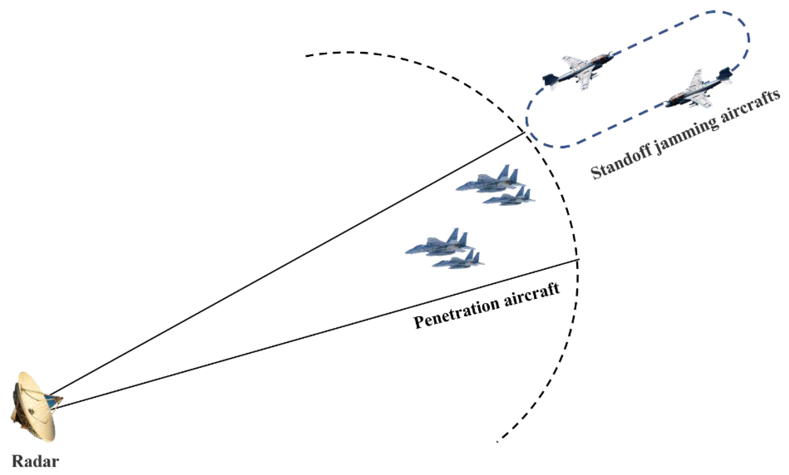
In order to seize the electromagnetic power and improve the survivability of the attack fighter formation, the electronic jammer formation and the attack fighter formation usually cooperate in a cooperative manner [41,42]. As one of the typical applications of Aviation Electronic Warfare, standoff jamming aircraft is outside the enemy defense circle, which provides support for the implementation of their own combat aircraft tasks by suppressing the enemy radar system. Usually, during the implementation of long-range support jamming, the mission aircraft flies in the direction of the target, while the jammer makes runway flight at a specific distance and height from the target. The basic situation map is shown in Figure 4.

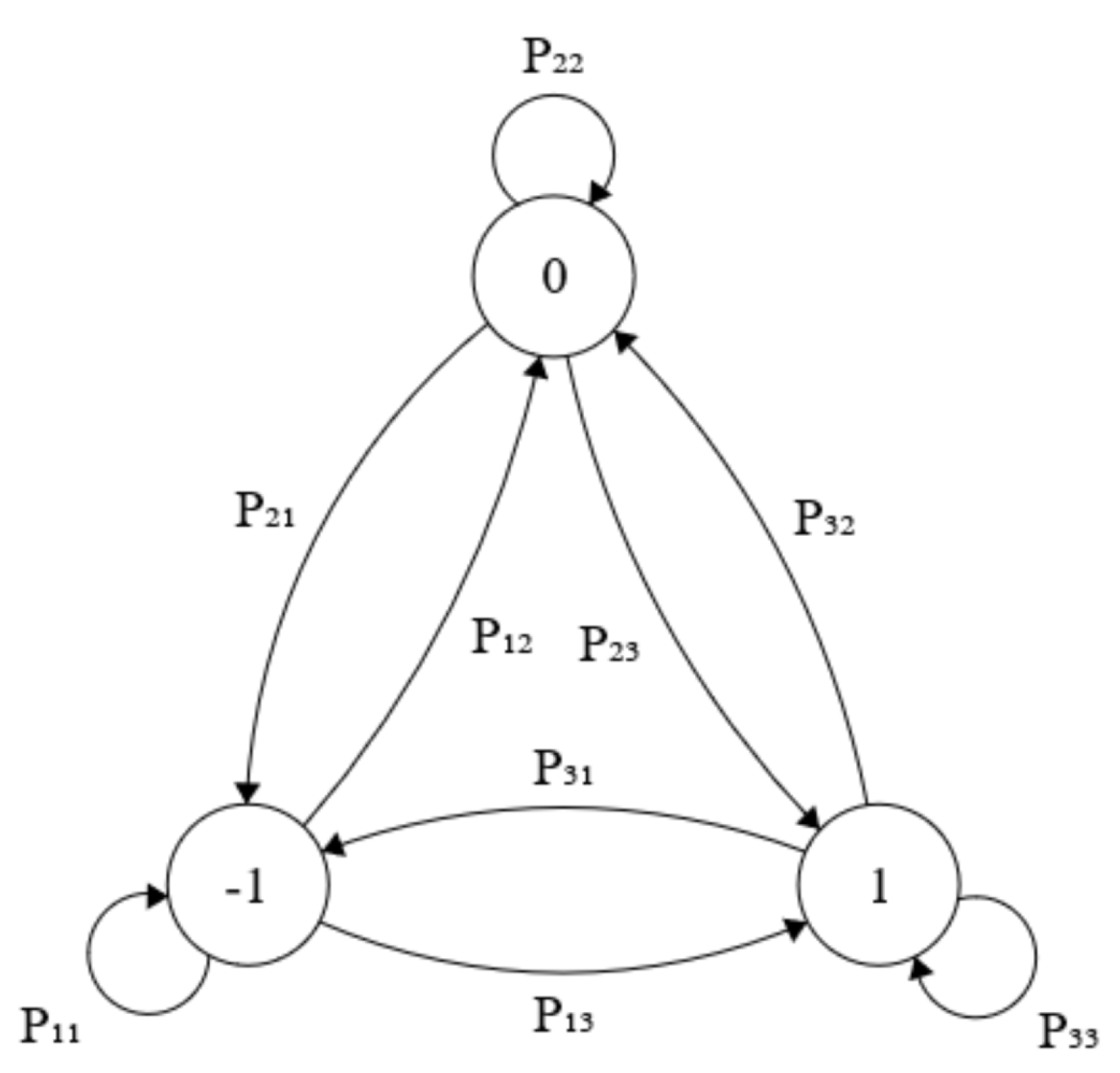
From the tactical perspective, there are three main conditions influencing the operation effect: Time Domain Conditions $f_1$: select the duration of the EW mission as the conditional state attribute. Depending on the actual situation of task duration overlap, ’−1’ indicates that duration cannot overlap, ’0’ indicates that duration partially overlaps, and ’1’ indicates that duration completely overlaps. The Markov process is a first-order Markov model, and the relationship between the state vector and the state transition probability is shown in Figure 5.

$$X\left(f_1\right)=\left\{a_1^{\left(1\right)}\right\}=\left\{b_1^{\left(1\right)},b_2^{\left(1\right)},b_3^{\left(1\right)}\right\}=\left\{-1,0,1\right\}$$

(58)

Spatial domain condition $f_2$: an important indicator of standoff jamming is its airspace coverage. Spatial coverage includes pitch coverage, instantaneous pitch coverage, azimuth coverage, instantaneous azimuth coverage, and so on. We select the beam width as the conditional state property. According to the beam coverage target situation, it can be divided into three attributes: not coverage (−1), partially coverage (0) and completely coverage (1). Specifically defined:

$$X\left(f_2\right)=\left\{a_1^{\left(2\right)}\right\}=\left\{b_1^{\left(2\right)},b_2^{\left(2\right)},b_3^{\left(2\right)}\right\}=\left\{-1,0,1\right\}$$

(59)

Energy domain condition $f_3$: since the jammer is far away from the target, the jamming power is also an important indicator for effectively shielding the aircraft from jamming. So, select power as condition state attribute. According to whether the power meets the demand or not, it is divided into two attribute states, not meeting power requirements (0) and meeting the power requirements (1). Specifically defined:

$$X\left(f_3\right)=\left\{a_1^{\left(3\right)}\right\}=\left\{b_1^{\left(3\right)},b_2^{\left(3\right)}\right\}=\left\{0,1\right\}$$

(60)

According to the EW Tactical Implementation Rules, only when all three of the above conditions are met will the tactical application be effective. If one condition is not satisfied or partially satisfied, it will affect the system effectiveness. The best effectiveness can only be achieved if all the conditional feature attributes of the system are satisfied.

Analysis shows that there are 18 possible combinations of satisfying states for the three conditional state attributes. To facilitate decision-making, these 18 states are divided into four levels according to Hypothesis 2: Excellent, Good, Medium and Poor. The detailed breakdown table is shown in

Table 1. Conditional state satisfies level table.

States Level	Possible Satisfaction States
Excellent	(0,1,1), (1,0,1), (1,1,0), (1,1,1)
Good	(0,0,1), (−1,1,1), (1,−1,1), (0,1,0), (1,0,0)
Medium	(−1,0,1), (0,−1,1), (−1,1,0), (0,0,0), (1,−1,0)
Poor	(−1,−1,1), (−1,0,0), (0,−1,0), (−1,−1,0)

.

According to the calculation, the approximation between the transition state and the expected state of the task unit is ${\eta }_j\left(\pi \right)=0.6283$. See Appendix A for calculation process.

Similarly, the approximation between the transition state and the expected state of the target unit is ${\eta }_k\left(\pi \right)=0.6324$. Taking $c_1=1$, $c_2=2.1$ and $c_3=8$, the degree of association between the task unit and the target unit is:

$$e_{j,k}=0.3155$$

(61)

In the process of cooperative operation between EW aircraft and penetration formation, the degree of correlation between EW aircraft and target unit will directly affect the decision-making implementation of penetration formation task. If only the value of correlation degree $e_{j,k}$ is given, it is not helpful for penetration formation and EW interference aircraft to grasp the situation of electromagnetic threat in the battlefield. Therefore, considering the practicability, feasibility and discrimination, this paper classifies the target unit into I to V levels according to the correlation degree from low to high after interference [43].

(1)

I-level threat. Level I threat is strongest and degree $e_{j,k}$ is $\left[0,0.2\right)$. The interference effectiveness is the lowest, the target unit is very threatened and the interference demand is urgent, so interference or attack measures should be taken immediately.

(2)

$II$-level threat. The $II$-level threat is stronger and the correlation degree $e_{j,k}$ is $\left[0.2,0.4\right)$. The interference effectiveness is lower and the target unit is more threatened. Compared with level I, there is a certain interference requirement. It is important to note that level $II$ threats should be given sufficient attention by penetration and EW formations, which often translate into I-level threats.

(3)

$III$-level threat. $III$-level threat is medium threat, and correlation degree $e_{j,k}$ is $\left[0.4,0.6\right)$. The jamming effectiveness is general, and the threat degree of target unit is moderate. Compared with I and $II$-level threats, the penetration formation needs moderate interference. At this time, it is necessary to observe the state change of the target unit at any time, so as to prevent it from transforming into I and $II$ level threats. It can also try to transfer the state of task unit, improve the jamming effectiveness and turn it into $IV$ and V-level threat.

(4)

$IV$-level threat. $IV$-level threat is weak threat, and correlation degree $e_{j,k}$ is $\left[0.6,0.8\right)$. The jamming effectiveness is good and the threat degree of target unit is small. The current jamming strategy can be maintained, or the state of task unit can be adjusted to turn it into V-level threat if the interference resources allow.

(5)

V-level threat. Level V threat is no threat and degree $e_{j,k}$ is $\left[0.8,1\right]$. The interference effectiveness is the best, and the target unit has the least threat to the penetration formation. At this point, the task unit only needs to maintain the current interference policy and pay attention to the state of the target unit.

From the results of the previous correlation calculation, $e_{j,k}=0.3155\in \left[0.2,0.4\right)$, at this time, the target unit is at level $II$ threat. The formation of electronic jamming aircraft should adjust the jamming strategy as soon as possible to improve the jamming effectiveness while keeping track of the target unit state. The jamming strategy can interfere with either the setting level of equipment parameters or the use of tactics. However, if we stand in the view of radar, the approximation is ${\eta }_k\left(\pi \right)=0.6324$ at this time, which is classified as level $IV$ threat according to the previous level, and in the view of EW system, the approximation is ${\eta }_j\left(\pi \right)=0.6283$ at this time, which is also level $IV$ threat, and the response strategy for level $IV$ threat is to maintain the current interference strategy. Obviously, it is easier to put penetration formations under threat from a single perspective than from the conflict association analysis in this paper.

This establishes the relationship between EW effectiveness measurement and decision-making from the perspective of conflict. By adjusting the state transition strategy, that is, the propensity of conditional state attribute transfer, the grey correlation degree between target unit and task unit state can be obtained during the operation of EW, and then the better performance of EW can be obtained by adjusting the use strategy of EW according to the threat level. Conflict state association analysis and evaluation process fully considers the states of both sides of the conflict in EW, effectively reflects the change and impact of the conflict states between the task unit and the target unit in the course of the application of EW, and the evaluation results are more credible than the single evaluation.

7. Conclusions

The EW Conflict System is a dynamic and complex system, which has different states at different times and converges to a certain confrontation state eventually. It has typical Markov chain characteristics. In order to evaluate effectiveness more scientifically, the following work has been carried out in this paper:

(1)

Defines the EW target unit system and task unit system as EW conflict system. The relationship between system elements is hierarchically analyzed to find the nature of the conflict. Conflict relationships between systems are mapped to conflicts between states to achieve a mapping description from system to state.

(2)

The basic criteria and conflict state hypothesis of effectiveness analysis are established. Based on the measurability analysis of conditional state attributes, the measurable conditional state space for EW conflicts is constructed. The formal description of EW conditional state transition track is analyzed.

(3)

By analyzing the uncertainty of EW conflict, the EW conflict state transition is described as a Markov random process. The relevant properties of Markov process dynamic transfer in the conflict state of EW are analyzed. The transition state probability description of the transfer process is analyzed.

(4)

The effectiveness of the EW system is evaluated based on the approximation of the transition state and the expected state. At the same time, through the model application of typical scenarios, the feasibility of the theory is verified.

Based on the above work, this paper effectively solves the limitations of understanding the connotation of effectiveness evaluation in the past and treats the same effectiveness under the same combat situation, and obtains the theoretical support for decision-making of task units in EW conflict system based on effectiveness evaluation.

With the implementation of the EW mission, the EW target unit will take some countermeasure to reduce the effectiveness of the EW task unit. Reflected in the EW task unit system, during the process of state observation, there may be insufficient observation data or observation data has some errors, noise, and so on, which results in inaccurate observation state, thus reducing the reliability of effectiveness evaluation results. This requires analysis and processing from two perspectives: how to compensate for data loss and how to process noise. In future studies, we will focus on how missing observations can be filled by entropy multiple imputation or clustering-based nearest neighbor algorithm, and explore the possibility of applying the Gaussian distribution statistical model to reduce the noise of the observed data. Through these two aspects of research, the theoretical system of EW effectiveness evaluation based on conflict state can be improved.