The Relationship of Causal Factors Affecting the Future Equilibrium Change of Total Final Energy Consumption in Thailand’s Construction Sector under a Sustainable Development Goal: Enriching the SE-VAR_X Model

Abstract

This study aims to analyze the influence of the relationship between causal factors that affect the future equilibrium of the total final energy consumption in the construction sector of Thailand under the sustainable development policy for the period of 10 years (2019–2028). This analysis was achieved with the application of the Structure Equilibrium-Vector Autoregressive with Exogenous Variables model (SE-VAR_X model). This model was developed to fill research gaps and differs from those of previous studies. In the selection of variables, the study focused on Sustainable Development (SD)-based variables available through the lens of Thailand. The exogenous variables included real GDP, population growth, urbanization rate, industrial structure, oil price, foreign direct investment, international tourist arrivals, and total exports and imports. Every variable had a co-integration at level (1) and was used to structure the SE-VAR_X model. This particular model can effectively analyze the influence of the direct relationship and meet the criteria of goodness of fit without spuriousness. This SE-VAR_X model allowed us to discover that every variable in the model had an influence on the equilibrium change, where the real GDP is the fastest variable to adjust to the equilibrium while the total final energy consumption has the slowest adjustment ability. The SE-VAR_X model can be used to project the total final energy consumption, as verified by the performance test result. The test was measured based on the Mean Absolute Percentage Error (MAPE) and Root Mean Square Error (RMSE), and their results were 1.09% and 1.01%, respectively. This performance result had the highest value compared to other models in the past. Thus, the SE-VAR_X model is suitable for forecasting over the next 10 years (2019–2038). The results of this study reveal that the total final energy consumption in the construction sector of Thailand will exhibit a continuously increasing growth rate from 2019 to 2028, amounting to about 144.29% or equivalent to 364.01 ktoe. In addition, the study also found that future government plans may be difficult to achieve as planned. Therefore, the introduced model should be integrated into national development planning and strategies to achieve sustainable development in the future and to enable its application to other sectors.

1. Introduction

Economic and social growth has seen gradual improvement in the current global climate. Many countries have made industrial development and global expansion possible. However, there is no doubt about the ongoing impact on fossil fuel consumption due to such growth. This has led to crisis in its quantity and price. Most importantly, it continues to impact the environment negatively. If we look at a global scale, China and parts of Europe, particularly those in the Organization for Economic Co-Operation and Development (OECD) [1], their economies are growing quickly, while their growth rate is soaring upward at the same time. In addition, for the OECD group members, the economies of these countries are growing rapidly with an annual growth rate of 2% [1,2]. One noticeable example is that of India where the population continues to increase [2]. Therefore, the growth in the economy and population will affect the global energy consumption at a growth rate of 0.9% (2017/2016), in which the oil consumption rate will become dominant and high [1,2]. The ongoing increase in global energy demand has had a large impact on the ecosystem, contributing to the unwelcoming phenomenon of climate change. As the CO₂ emissions keep increasing, so does the greenhouse effect at the same time [3]. However, although many countries have implemented various policies and collaborated between one another to reduce greenhouse emissions, the issue remains unresolved and adds no value in terms of sustainability. As for Thailand, it is one of many other countries willing to cooperate and take initiative to address the problem. One such action is the country’s participation and involvement in the United Nations Framework Convention on Climate Change, Kyoto Protocol, and Paris Agreement [1,3] in order to provide a better framework for achieving sustainable development.

Today, Thailand has put policies in place to accelerate economic development, aiming towards developing a country where the economic, social, and environmental development is emphasized based on national sustainable development policies and strategies. This serves for the short term of 1 to 5 years, the medium term of 6 to 10 years, and the long term of 11 to 20 years. The above development has been set forth through the promotion and acceleration of overall development in all aspects [4], including the promotion of foreign direct investment, urbanization, and industrial structure in all major areas. There is also foreign encouragement in the tourism industry and a focus on export activities. Additionally, the government promotes the increment of wages and intervenes in securing the oil and diesel prices, while a special fund has been established to support various industries. Comparing 2017 to 2016, with the abovementioned polices, Thailand has continued to grow with an economic growth rate of 4.5%. Moreover, the social growth rate was seen to rise to 2.59%. This success has been reported from 2000 to 2017 [4,5].

However, the economic and social development of Thailand does have an effect on the environment as well; the amount of CO₂ emissions from the national energy consumption increased by 1.5% in 2017 compared to 2016 [1,5]. In particular, the construction sector emits a high volume of CO₂ emissions. This reflects that the ecological system is affected, and greenhouse gas emissions continue to increase, mainly contributed by the construction sector. In addition, methane (CH₄) is ranked as having the second highest emission levels [3,5]. This impact deteriorates the environmental system, though the government has tried to implement measures and strategies to minimize the impact on the environment. In the context of Thailand, the government has undertaken many initiatives in terms of supportive policies to reduce energy consumption, be it through promotional or penalty policies. However, energy consumption and CO₂ emissions continue to increase regardless, especially energy consumption in the construction sector on what appears to be a daily basis. This reflects the historical absence in Thailand of an important and effective tool and measure to formulate accurate and effective policies. Based on the relevant studies available in Thailand, spurious models continue to be applied, and such applications result in the failing of the policies implemented in all application terms. Concerning the sustainable development goal of 1 to 5 years, to support the medium term of 6 to 10 years and the long term of 11 to 20 year in Thailand, the efforts to meet this goal seem unsuccessful due to limited implementation tools for effective forecasting that can be universally applied to different sectors. Thus, this study aims to fill this gap, so Thailand can perform better in national strategic planning. Therefore, we attempted to develop a Structure Equilibrium-Vector Autoregressive with Exogenous Variables (SE-VAR_X) model for such planning. After reviewing various relevant studies, we found that the SE-VAR_X model is a model that differs from other models in the past, and it is an ideal model to be deployed in different contexts and sectors.

In this section, a number of well-known studies are revisited in order to investigate the causal relationships between various factors through different research methods and techniques. Also, in the establishment of this paper’s model, many literature sources have been discussed to identify and support the model with relevant contributions in terms of the Structure Equation Model. Ashley and Tsang [6] proposed a testing procedure using cross-sample validation (CSV) to analyze the credible Granger-causality. The findings reveal that the price in regards to power, based on the in-sample Granger-causality F test, is controllable. As investigated by Yu and Yang [7], the causality between both linear and nonlinear process variables was studied by proposing a transfer entropy with an optimization of binary alarm series. The results of this study’s analysis provide evidence of method suitability for industrial situations that are interfered with by noise. Ghafele and Gibert [8] analyzed the impact of fair use policy relative to the growth in private copying technology and the copyright markets of Singapore by referring to a method of differences-in-differences (DiD). This study affirmed a correlation between fair use policy with faster growth rates in the studied industries, but it did not show such a correlation with higher growth in the copyright industries.

Liu et al. [9] attempted to structure a method of Economy-Society-Ecology (ESE) subsystems by using a fuzzy analytical hierarchy process (FAHP), and entropy method (EM) to support the urbanization process of Chengdu, China. The study found that such a subsystem has a smaller effect on the coupling coordinated system while it is being enhanced with its ideal outputs for healthy urban development. Wang et al. [10] tried to justify the impact of changing urban forms on CO₂ emissions from commuting workers in Beijing by proposing an integrated analytical framework. The study’s results illustrated the great impact of such a change in terms of increased transport CO₂ emissions. In addition, the change relative to a more decentralized urban area has a greater impact in the above matter, resulting in a large rise in CO₂ emissions.

Also, [11] investigated the connection between water use change, urbanization and economic growth in China from 1997 to 2013 by applying a co-integration test and a VECM (vector error correction model). This study provided evidence of the existence of a long-run equilibrium relationship among those indicators, while the short-run effects and Granger causal relationship were found to be insignificant. This implies that a water crisis is likely to arise as a result of urbanization and economic growth. In the same case study of China, [12] explored the link between economic, construction land use and ecology subsystems in Zhejiang from 2000 to 2012 by optimizing a Granger test and a coupling coordination model. The results of the study demonstrate that the changes in value of the economic subsystem are the cause of changes in the ecology and construction land use (CLU) subsystems, while the changes of value of the ecology and CLU subsystems are the root cause of each other. In addition, Liu et al. [13] explored the trends between Rural-to-Urban Migrants (RUMs) and Urban Land Expansion (ULE) in Hubei, China from 2009 to 2014 by applying a decoupling model. The study concluded that an irregularly distributed large percentage of the rural population was moving to urban areas, and that urban land use is both rising rapidly and is inefficient.

Ameyaw and Yao [14] analyzed the relationship between Gross Domestic Product (GDP) and CO₂ emissions from 2007 to 2014 in five West African countries. They also proposed a non-assumption driven forecasting technique by using a bidirectional long short-term memory (BiLSTM) sequential algorithm formulation to forecast the long-term total CO₂ emissions from 2015 to 2020. Their results indicated the presence of a unidirectional relationship between GDP and CO₂ emissions. Also, they were able to suggest sustainable policy targets based on CO₂ emissions projections. Zhixin and Xin [15] investigated the causal link between energy consumption and economic growth of Shandong, China, from 1980 to 2008, by implementing a Generalized Least Square (GLS) method, which concluded that a long-term relationship between these two factors exists, implying that the economic growth of the studied area is dependent on energy consumption. Du et al. [16] applied the Bernoulli–Nash Social Welfare Function (BNSWF) to examine the effects of the emission cap on emission-dependent manufacturers’ decision-making. The study shows that the system-wide and manufacturer’s profits are enhanced with such an emission cap, while the permit supplier is found to decline. However, it is suggested that the manufacturer and permit supplier can increase the profit through coordination in the supply chain.

In the USA, Yildirim et al. [17] explored the casual relationship between energy consumption and economic growth by using the Toda-Yamamoto procedure and bootstrap-corrected causality test. The study illustrated that there is a causal relationship between biomass-waste-derived energy consumption and real GDP, suggesting that the USA should focus on energy production from waste as an additional energy resource. Madlener and Sunak [18] applied different processes and mechanisms of urbanization to investigate the influences of urbanization on urban structures and energy demand. They found that urban energy demand has risen significantly, and the fuel mix tends to change because of different mechanisms of urbanization within various economic sectors. Al-mulali [19] analyzed the influence of nuclear energy consumption on GDP growth and CO₂ emissions by conducting a panel data analysis in 30 major nuclear energy-based countries from 1990 to 2010. The study concluded that there is a positive long-run effect of nuclear energy consumption on GDP growth, but not on CO₂ emissions. Furthermore, Cutlip and Fath [20] investigated causality between carbon emissions and economic development through a study of case studies in six countries. This investigation showed a connection between those variables.

Bernstein and Madlener [21] forecasted both short-and-long term electricity demand elasticities for the German manufacturing industry at different sub-sectoral levels through a co-integrated VAR method. As a result, they found a long-term relationship for five studied subsectors. Additionally, they concluded that a sub-sectoral approach is an ideal method for the estimation of electricity demand elasticities. In Lebanon, [22] assessed the connection between energy consumption and economic growth from 1980 until 2009 by deploying various causality tests, including the Hsiao, Toda-Yamamoto, and vector error correction-based Granger causality tests. Their study revealed a bidirectional short-and-long term relationship. This implies that energy is a vital source for the economic growth of Lebanon. In assessing the impact of energy consumption and CO₂ emissions on the development of economy and finance, Al-mulali and Che Sab [23] selected 19 countries with an application of a panel model covering the period of 1980 to 2008. The assessment provides evidence of energy consumption contributing to the studied development. However, the study found that the high levels of said development have increased CO₂ emissions.

In an attempt to comprehend the connection between urbanization and economic development in China, Chen et al. [24] took a sample of 31 provinces through a method of quadrant mapping. This study showed that the relationship between those two variables is similar to the Matthew effect. Also, at a provincial level, such a relationship exists with a significant difference. Jiao and Yang [25] analyzed the relationship between the economic development and carbon emissions in western China by implementing an econometric FGLS (Feasible generalized least squares) analysis. The study found the presence of a positive correlation between carbon emissions and industrial transformation and a rise of consumption as parts of economic factors. In particular, the significance of such a correlation is found after the implementation of the Western development strategy. Also, Liu and Lathrop [26] tried to detect newly urbanized areas by applying an artificial neural network. This case study produced a result of 20–30% accuracy with its method while reducing the computational cost. Williams, Hahs and Vesk [27] tried to discover the relationship between plant traits and the urban environment by doing a synthetization of study results and an examination of plant traits or niche indicators of urban flora. Their study found an increase of niche indicators for nutrients, temperature and alkalinity across many studies.

In the next line of studies, different studies applied different techniques, and structural equation modeling is an ideal method among them, enabling the success of this paper. Ye et al. [28] studied transfer commuting attitudes in Nanjing, China, by applying a method of market segmentation consisting of K-means clustering, factor analysis and structural equation modelling (SEM). The study found that sensitivity to time is found to be the vital factor affecting transfer willingness. Liu and Yang [29] tried to identify factors that affect behavioral intention (BI) toward the sharing economy by expanding on the technology acceptance model. Throughout their study, they found that perceived usefulness (PU) and perceived ease of use (PEOU) are observed to be the key factors affecting BI. Shih [30] did a study to identify the determinants of different factors: enterprises’ strategic orientations, competitive advantages, radical innovation and business performance with a sample of 86 firms via regression analysis using the PLS SEM model. This study concluded that a firm’s radical innovation capability and adoption can be enhanced through either market orientation factor or entrepreneurial orientation factor, while brand advantage has a significant impact on firms’ performance. Also, [31] attempted to determine the determinants of effective Lean Manufacturing by applying the method of Covariance-based Structural Equation Modeling (CB-SEM) analysis. Their findings showed that those determinants can be used as guidelines to attain LM effectiveness, including a provision of necessary steps for successful lean implementation and achievement of lean cost reduction and time-saving. Grewal et al. [32] did a study to detect multicollinearity and measurement error in structural equation models in the theory testing by conducting a Monte Carlo simulation. Their analysis explained multicollinearity may become an error when the multicollinearity is extreme, between 0.6 and 0.8 and between 0.4 and 0.5. In Malaysia, Habidin et al. [33] conducted a confirmatory factor analysis for sustainable manufacturing practices in the automotive industry of Malaysia by applying the SEM technique. At the end of the research, they concluded that those automotive manufacturers are found to be intrigued by and involved in sustainability. They were observed to have a clear integration between sustainability and their business strategy.

Jiao et al. [34] deployed a novel approach for the estimation of sustainable urbanization performance in 31 provinces of China using SEM. Their findings suggest that effective policies and strategies can be improved through the assessments of the study in order to improve urban sustainability. Bandalos [35] examined the preciseness and utility of overall error and error estimators in the structural equation models by using the Monte Carlo method. This study showed that the rescaled non-centrality parameter and a sample estimator of overall error (EFo) produced a highly precise estimate of the approximation error and overall error amount, respectively. Shen et al. [36] produced a ranked list of the sustainable performance of urbanization in the prospect of global view between 111 countries, with data retrieved from the World Bank database and the United Nation database. Their study provides a referential outcome in which a difference in urbanization will contribute to a varied level of sustainable performance. Woo [37] revisited the international economic policy of China after three decades of its transformation and opening regionally and globally. His analysis shows evidence of negative spillovers due to large trade surpluses and greenhouse gases. Also, Liang et al. [38] developed a principal component analysis (PCA) and used Grey TOPSIS methodology to measure the sustainable urban development capacity of 13 cities of Jiangsu, China. In the study, an index system is established, and its measurement result has shown that all kinds of index weights in the measurement are able to increase in the comprehensive and persuasive assessment results.

Meulemans et al. [39] studied the occurrence of exercise dependence and eating disorders in the different genders of young adults by a Path analysis optimizing a Structural Equation Modeling (SEM). The findings have shown a small direct impact of gender on eating disorders. Han et al. [40] explored the factors affecting travel mode choice behavior in Jinan city of China by deploying a SEM-Logit Integration model. Their study found that gender, monthly income, trip purpose, travel distance, safety and convenience service are found to have a great impact on the selected traveling mode. Cheng et al. [41] proposed a structural equation model (SEM) to evaluate factors that influence passenger satisfaction towards the bus transfer process in China, and found bus fare and transfer distance are found to be the most influential factors for passenger satisfaction. Furthermore, Wang et al. [42] aimed to discover potential factor mechanisms of the long-distance travel mode choice by adapting a Structural Equation Model with a variance (ANOVA) approach. The study’s findings indicate that all factors except gender, service demand for safety, and departure time have a significant impact on the travel mode choice. Furthermore, they also illustrated that travel distance is found to be the top most influential variable on the choice of travel mode, while the service demand, performance evaluation, and personal attributes are the next most influential factors. Geng et al. [43] examined the effect of multiple motivations, government procedures, and demographic features on residents’ travel mode choice in Jiangsu Province, China, by structuring a multinomial logistic regression model with 1244 urban residents in total. Their analysis revealed that a pro-environmental motivation plays a great role in the promotion of green travel mode choices compared to car use, yet it is driven by self-interested motivations rather than pro-environmental motivation. Other variables, like gender, age, vehicle ownership, travel distance, income and government instruments have a great impact on the travelling mode choices.

Dobrovolskienė et al. [44] attempted to identify what enables project managers to achieve sustainability in their decision-making in the construction and automotive industry of Lithuania. The study shows that these managers are not that concerned with sustainability, and few sustainability criterions are put in place. However, their concern is greater than their team members. Prause and Atari [45] investigated the connections between networking, organizational development, structural frame conditions and sustainability under the concept of Industry 4.0 by applying a method of semi-structured expert interviews among a set of samples of high-tech manufacturing corporations in Estonia. Based on their findings, a poor organizational environment causes a negative effect on the performance of a networked construction, apart from technical matters. Additionally, Vegera et al. [46] conducted a study to determine the stages of the technological cycle and their accounting objects of the industrial waste. In their study, “Appearance” is found to be the first stage, while “Collection”, “Accumulation”, “Waste Preparation for Use”, “Storage”, “Use” and “Burial” are the stages that follow. In addition, the waste of ferrous and non-ferrous metals, construction waste, waste due to reservoirs cleaned and costs are the accounting objects found in the cycle. Yevhen et al. [47] studied the role of industrial ecology and logistics to achieve regional sustainable development goals. Upon their analysis, the integration of the environmental vision with economic content becomes the foundation of policy formulation and implementation to attain the above goals. Fomina et al [48] sought to understand the essence of industrial cooperation, and examined its influence on the growth of a sustainable economy by using a log-linear model. The investigation’s results showed that an additional growth in the economy of about 2.3–3.0% is provided by the industrial cooperation. Meanwhile, such a system of cooperation helps boost the factor impact of economic growth determinants. Lastly, Oganisjana et al [49] analyzed three-stage research based on a social innovation project urging people to get involved in tackling social problems. As for the study’s results, the intrapersonal, interpersonal and external factors were found to be motivational drivers for people to get involved in solving the problems.

The review of relevant research revealed that most modeling structures are no different from one another, and some models are buggy and produce potential errors if applied to other sectors or contexts. Thus, we introduced the SE-VAR_X model to fill the above gap as well as to provide maximum efficiency and effectiveness in application. The SE-VAR_X model was developed for medium- and long-term forecasting, yet was found to be the best model. We used the time series data for the period 1990–2017, and applied linear structural relations (LISREL, version 9.2, Chicago, IL, USA) software in later estimations. The research process is shown below.

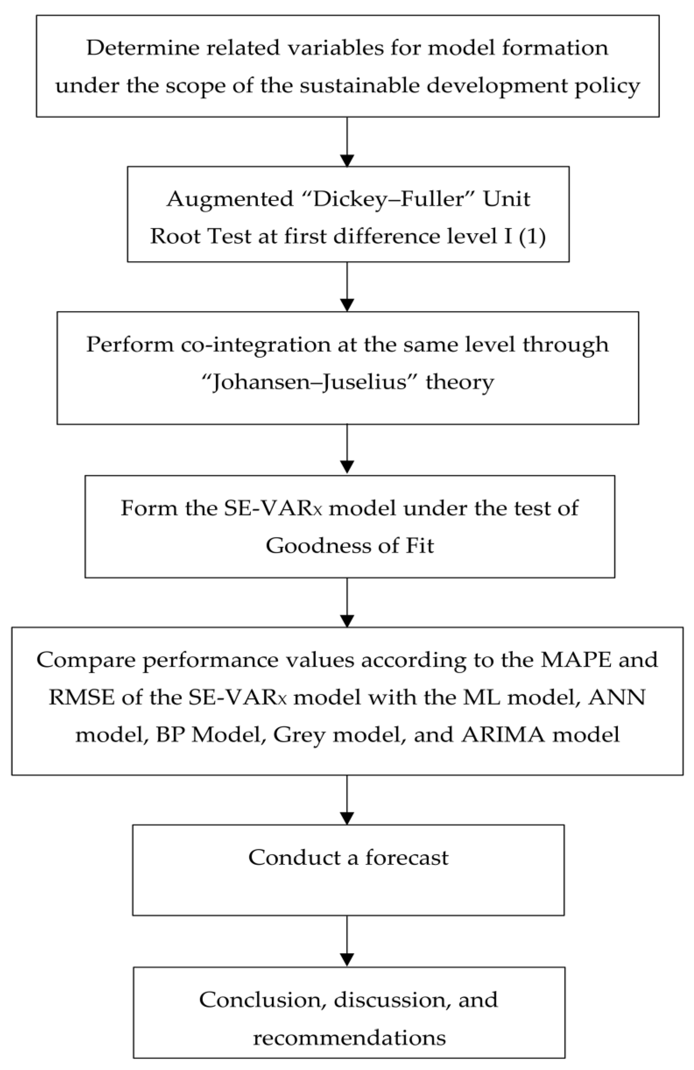
• Determine all variables for the SE-VAR_X model so as to analyze the influence of the relationship between causal factors affecting the equilibrium adjustment of the total final energy consumption based on the sustainable development policy for 10 years (2019–2028). This process applies Augmented Dickey–Fuller theory [50,51] along with the concept of walk drift and time trend at the first difference using data from 1990 to 2017.
• Take stationary variables at the first difference for a co-integration test based on the Johansen-Juselius concept [52,53].
• Construct the SE-VAR_X model to analyze the influence of the relationship in both the long term and short term.
• Testify the performance of the SE-VAR_X model based on the value of the Mean Absolute Percentage Error (RMSE) and Root Mean Square Error (RMSE) [54,55], and compare them with the same sort of values in Multiple Linear Regression model (ML model), Artificial Neural Network model (ANN model), Back Propagation neural network model (BP model), Grey model, and Autoregressive Integrated and Moving Average model (ARIMA model).
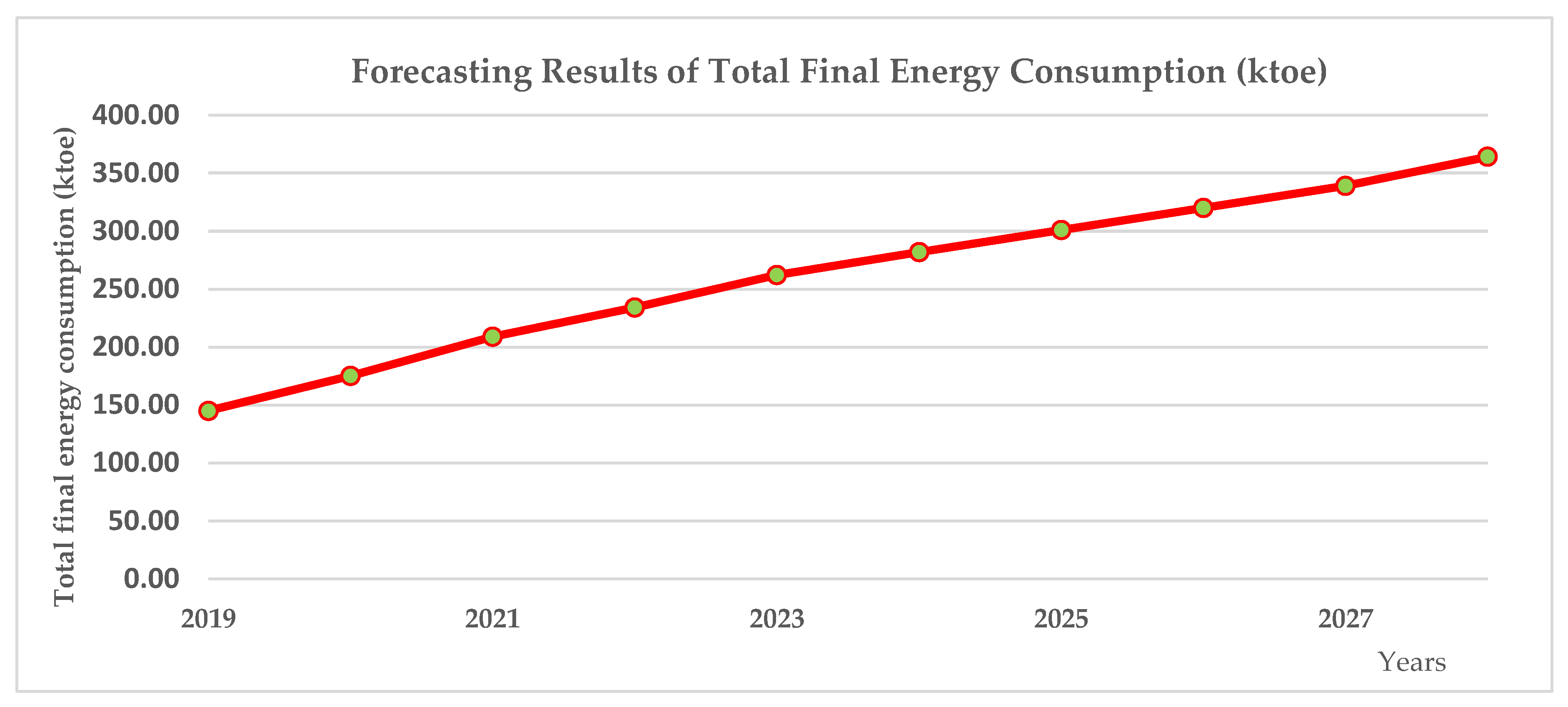
• Forecast the total final energy consumption by using the SE-VAR_X model for the years 2019–2028, totaling 10 years. The flowchart of the SE-VAR_X model is shown in Figure 1.

The remainder of this paper is as follows: Section 2 discusses the materials and methods. Section 3 shows the results. Section 4 summarizes the conclusion and discussion.

2. Materials and Methods

2.1. Stationary Features

The data used to structure the SE-VAR_X model have to be selective and identified as stationary. This selection is illustrated below.

If $Y_t$ is a stochastic variable time series and stationary, it must consist of three properties as shown in Equations (1)–(3).

The equation with a mean has to be as follows:

$$E\left(Y_t\right)=E\left(Y_{t-k}\right)=\mu$$

(1)

The equation with a variance becomes as follows:

$$Var(Y_t)=E{(Y_t-\mu )}^2={(Y_{t-k}-\mu )}^2={\sigma }^2$$

(2)

The equation with a covariance can be displayed as below:

$$E\left[{\left(Y_t-\mu \right)}^2{\left(Y_{t-k}-\mu \right)}^2\right]={\gamma }_k$$

(3)

The height or spacing of covariance values is the same. The distance between the two $Y_t$ values does not depend on time. These three properties are referred to as stationary.

The stationary stochastic process or stationary is a time series of mean or expected values, as well as the values of a variance and a covariance (constant overtime). It does not depend on time, but rather on the distance or lag.

The Dickey–Fuller concept has been used to solve non-stationary data problems in the form of a difference regression called the first-order autoregressive process, via one of the following three equations:

$$\Delta Y_t=\delta Y_{t-1}+{\epsilon }_t$$

(4)

$$\Delta Y_t={\alpha }_1+\delta Y_{t-1}+{\epsilon }_t$$

(5)

$$\Delta Y_t={\alpha }_1+{\alpha }_{2}T+\delta Y_{t-1}+{\epsilon }_t$$

(6)

where $\Delta Y_t$ represents the variables to be studied, $\delta$ is the coefficient of the lag, and ${\epsilon }_t$ is the error term with normal distribution. The mean = 0, the variance = ${\sigma }^2$ for the hypothesis of the unit root test, and it is denoted as $H_0$:$\delta$ = 0, non-stationary, $H_a$:$\delta$ < 1, stationary.

$\Delta Y_t$ will be qualified as on-stationary when accepting $H_0$ and the variance $\delta$ is increased exponentially or explosively when the time increases. Details of each model can be shown as follows:

$$\Delta Y_t=\delta Y_{t-1}+{\epsilon }_t$$

(7)

Equation (7) is a simple model with a mean of zero suitable for data with a mean of only zero. The model was modified by adding a drift term in the following equation:

$$\Delta Y_t={\alpha }_1+\delta Y_{t-1}+{\epsilon }_t$$

(8)

where ${\alpha }_1$ is the drift term.

Equation (8) can also improve the unit root test as a component of Trend Stationary (TS) and Difference Stationary (DS) processes, as in the following equation:

$$\Delta Y_t={\alpha }_1+{\alpha }_{2}T+{\epsilon }_t$$

(9)

where $T$ is the time trend, ${\alpha }_2$ is the coefficient of the trend.

${\epsilon }_t$ has a stationary feature with a mean of 0, and the variance is equal to ${\sigma }^2$.

However, causing the time series to make the first difference or higher difference will make the serial data available as a stationary through the difference stationary method, as follows:

$$\Delta Y_t={\alpha }_1+{\alpha }_{2}T-\delta Y_{t-1}+{\epsilon }_t$$

(10)

In Equation (10), the amount of time increases with the increasing level. If rejecting $H_a$ or accepting $H_0$ indicates that the data are non-stationary, then the coefficient $\delta =0$ is significant. This shows that the tau statistics of the coefficients calculated in the absolute term are less than the Dickey–Fuller (DF) critical in the absolute term. In this case, it shows that ${\epsilon }_t$ has no white noise feature and it shows that the analyzed data have an autocorrelation feature where the Augmented Dickey–Fuller (ADF) Test must be used with the assumptions and goodness of fit, as also used in similar tests. The equation was modified by increasing the number of lagged variables of the dependent variable in a higher order to eliminate the problem of autocorrelation shown in the format as follows:

Hypothesis of unit root test: $H_o$:$\delta$ = 0, non-stationary, $H_a$:$\delta$ < 1, stationary.

At level, if reject $H_o$ that the data are stationary. The White Noise or time series of variables is stationary, which shows that the $\Delta Y_t$ integrated at d or written in the symbol $\Delta Y_t~I(d)$.

$$\Delta Y_t=\delta Y_{t-1}+{\displaystyle \sum _{i=2}^p{\beta }_i\Delta Y_{t-i+1}}+{\epsilon }_t$$

(11)

$$\Delta Y_t={\alpha }_1+\delta Y_{t-1}+{\displaystyle \sum _{i=2}^p{\beta }_i\Delta Y_{t-i+1}}+{\epsilon }_t$$

(12)

$$\Delta Y_t={\alpha }_1+{\alpha }_{2}T+\delta Y_{t-1}+{\displaystyle \sum _{i=2}^p{\beta }_i\Delta Y_{t-i+1}}+{\epsilon }_t$$

(13)

where $\Delta$ is the lagged values of the first difference of the variable.

Equations (11)–(13) show that the most appropriate form of equation is the Augmented Dickey–Fuller, as shown in Equation (14).

$$\Delta Y_t={\alpha }_1+{\alpha }_{2}T+\delta Y_{t-1}+{\displaystyle \sum _{i=2}^p{\beta }_i\Delta Y_{t-i+1}}+{\epsilon }_t$$

(14)

However, the DF and ADF equations do not differ significantly, as the aim of the ADF is to solve the problem of error term and turn it into the feature of white noise or to have an error term of zero mean.

2.2. Co-Integration Test

This distance is stationary or symbolized as $Y_t-{\beta }_2{X}_t~I(0)$, $Y_t-{\beta }_2{X}_t=u_t$ and for time series $Y_t$ and $X_t$ has a stationary spacing model, which shows that the values of both variables are moving in one direction, not in different directions. This is because the two time series share a common stochastic trend, which we will call vector $\left[\begin{array}{c}1\\ -{\beta }_2\end{array}\right]$ also written as ${\left[1-{\beta }_2\right]}^{\prime }$ showing a co-integrating vector. Moreover, the equation $Y_t-{\beta }_2{X}_t=u_t$ is referred to as a co-integrating regression. $Y_t$ and $X_t$ are in the following equations:

$$Y_t={\mu }_t+{\epsilon }_{Yt}$$

(15)

$$X_t={\mu }_t+{\epsilon }_{Xt}$$

(16)

where ${\mu }_t$ is a random walk but is a random walk but ${\epsilon }_{Xt}$ and ${\epsilon }_{Yt}$ are white noise. We use Equations (15) and (16) to find the values of $Y_t$ and $X_t$ as follows:

$$Y_t-X_t=({\mu }_t-{\mu }_t)+{\epsilon }_{Yt}-{\epsilon }_{Xt}$$

(17)

$$Y_t-X_t={\epsilon }_{Yt}-{\epsilon }_{Xt}$$

(18)

From Equation (18), when ${\epsilon }_{Yt}$ is the White Noise, it is still White Noise. The time ${\epsilon }_{Xt}$ series $Y_t-X_t$ is a time series that is stationary where the vector showing the long-run equilibrium is $\left[\begin{array}{c}1\\ -1\end{array}\right]$ or written as ${\left[1-1\right]}^{\prime }$. If $Y_t$ and $X_t$ have long-term equilibrium relationships or co-integration, they must have a coefficient ${\beta }_t$ which is not equal to zero, causing the following results. If the linear result of $Y_t$ and $X_t({\beta }_1{Y}_t+{\beta }_2{X}_t)$ is stationary, we call ${\left[{\beta }_1-{\beta }_2\right]}^{\prime }$ the co-integration vector, and we can find the error correction model as follows:

$$Y_t-Y_{t-1}={\epsilon }_t+{\phi }_1(Y_{t-1}-X_{t-1})$$

(19)

$$X_t-X_{t-1}=w_t+{\phi }_2(Y_{t-1}-X_{t-1})$$

(20)

where ${\phi }_1(Y_{t-1}-X_{t-1})$ and Equilibrium Correction Mechanism (or Error Correction ${\phi }_2(Y_{t-1}-X_{t-1})$ Mechanism) and Equations (19) and (20) are the short-term adaptive model for long-run equilibrium (Error Correction Model: ECM). Using the least squares method with the ECM model is not a spurious regression because all the dependent, independent and random variables are all stationary.

2.3. A Forecasting Model Using the SE-VAR_X Model

Concerning the SE-VARx model, we adapted the concept of the basic models, including the Structure Equilibrium-Vector Autoregressive model with exogenous variables. This SE-VAR_X model employs stationary variables at the first difference with a co-integration characteristic based on Johansen’s concept in order to analyze both the short- and long-term relationships of each variable in the model. Here, each causal factor has a direct effect, and is later used to construct the SE-VAR_X model as explained below.

$$X_t={\alpha }_0+{\alpha }_i{\displaystyle \sum X_{t-p-1}}+{\displaystyle \sum _{i=1}^p{\beta }_i{Y}_{t-i}+}{\displaystyle \sum _{i=1}^p{\delta }_{i}EC{T}_{t-i}}$$

(21)

where ${\alpha }_0$ is constant, ${\alpha }_i,{\beta }_i,{\delta }_i$ are parameters, ${\displaystyle \sum _{i=1}^p{Y}_{t-i}}$ represents the exogenous variables, which are stationary at level, and ${\displaystyle \sum _{i=1}^{p}EC{T}_{t-i}}$ represents the error correlation mechanism test.

Therefore, this study made the SE-VAR_X model applicable to forecasting the total final energy consumption in the construction sector as demonstrated below.

$$\begin{gathered} \Delta \ln (FEC)={\alpha }_0+{\alpha }_1{\displaystyle \sum \Delta \ln {(FEC)}_{t-p-i}}+{\beta }_1{\displaystyle \sum \Delta \ln {(GDP)}_{t-i}}+{\beta }_2{\displaystyle \sum \Delta \ln {(P_g)}_{t-i}}+{\beta }_3{\displaystyle \sum \Delta \ln {(U_r)}_{t-i}} \\ +{\beta }_4{{\displaystyle \sum \Delta \ln (I_s)}}_{t-i}+{\beta }_5{\displaystyle \sum \Delta \ln {(O_p)}_{t-i}}+{\beta }_6{\displaystyle \sum \Delta \ln {(F_i)}_{t-i}}+{\beta }_7{{\displaystyle \sum \Delta \ln (I_t)}}_{t-i}+ \\ {\beta }_8{{\displaystyle \sum \Delta \ln (X_m)}}_{t-i}+{\delta }_{1}EC{T}_{t-1} \end{gathered}$$

(22)

2.4. Measurement of the Forecasting Performance

In the measurement of the model performance, we employed the concepts of Mean Absolute Percentage Error (MAPE) and Root Mean Square Error (RMSE). This was done by comparing the forecasting result and accuracy of each model [54,55]. The calculation equations are displayed below.

$$MAPE=\frac{1}{n}{\displaystyle \sum _{i=1}^n\left|\frac{{\widehat{y}}_i-y_i}{y_i}\right|}$$

(23)

$$RMSE=\sqrt{\frac{1}{n}{\displaystyle \sum _{i=1}^n{\left({\widehat{y}}_i-y_i\right)}^2}}$$

(24)

3. Empirical Analysis

3.1. Screening of Influencing Factors for Model Input

The variables used in the model had to be screened and specifically selected. For the SE-VAR_X model, we selected variables relevant to the sustainable development policy in the construction sector by optimizing the time series data of the period of 1990 to 2017. In this study, nine variables were taken for analysis: the total final energy consumption ($FEC$), real GDP ($GDP$), population growth ($P_g$), urbanization rate ($U_r$), industrial structure ($I_s$), oil price ($O_p$), foreign direct investment ($F_i$), international tourist arrivals ($I_t$), and total exports and imports ($X_m$). Each of those variables was stationary at the first difference, as verified by the Augmented Dickey–Fuller unit root test shown in

Table 1. Augmented Dickey–Fuller unit root test at first difference I(1).

Tau Test at First Difference I(1)		MacKinnon Critical Value
Variables	Value	1%	5%	10%
$\Delta \ln (FEC)$	−5.96 ***	−5.05	−4.75	−3.50
$\Delta \ln (GDP)$	−5.84 ***	−5.05	−4.75	−3.50
$\Delta \ln (P_g)$	−5.25 ***	−5.05	−4.75	−3.50
$\Delta \ln (U_r)$	−5.77 ***	−5.05	−4.75	−3.50
$\Delta \ln (I_s)$	−6.05 ***	−5.05	−4.75	−3.50
$\Delta \ln (O_p)$	−5.39 ***	−5.05	−4.75	−3.50
$\Delta \ln (F_i)$	−5.71 ***	−5.05	−4.75	−3.50
$\Delta \ln (I_t)$	−5.44 ***	−5.05	−4.75	−3.50
$\Delta \ln (X_m)$	−5.70 ***	−5.05	−4.75	−3.50

Note: $\ln (FEC)$ is the natural logarithm of total final energy consumption, $\ln (GDP)$ is the natural logarithm of real GDP, $\ln (P_g)$ is the natural logarithm of population growth, $\ln (U_r)$ is the natural logarithm of urbanization rate, $\ln (I_s)$ is the natural logarithm of industrial structure, $\ln (O_p)$ is the natural logarithm of oil price, $\ln (F_i)$ is the natural logarithm of foreign direct investment, $\ln (I_t)$ is the natural logarithm of international tourist arrivals, $\ln (X_m)$ is the natural logarithm of total exports and imports, *** denotes significance at α = 0.01, and $\Delta$ is the first difference. Sources (own research).

.

Table 1 indicates the result of the unit root test, and this affirms that the tau test value of all variables is greater than the MacKinnon critical value. This implies a stationary character at level (1) with a significance of 1% of those variables. Consequently, we subjected those variables to a co-integration test, as suggested by Johansen and Juselius, to analyze the long-term relationship of each variable at the same level, as illustrated in

Table 2. Co-integration test by Johansen and Juselius.

Variables	Hypothesized Number of CE(S)	Trace Statistic Test	Max-Eigen Statistic Test	MacKinnon Critical Value
				1%	5%
$\Delta \ln (FEC)$, $\Delta \ln (GDP)$, $\Delta \ln (P_g)$, $\Delta \ln (U_r)$, $\Delta \ln (I_s)$, $\Delta \ln (O_p)$, $\Delta \ln (F_i)$, $\Delta \ln (I_t)$, $\Delta \ln (X_m)$	None ***	225.11	132.70	15.05	12.50
	At Most 1 ***	70.09	49.02	5.05	3.75

Note: *** denotes significance at α = 0.01. Sources: own research.

.

3.2. Analysis of Co-Integration

Table 2 indicates the co-integration of every variable since the values of the trace test at the first difference are 225.11 and 70.09, which are higher than the MacKinnon critical values at significance levels of 1% and 5%, respectively. The maximum eigenvalue test results are 132.70 and 49.02, which are higher than the MacKinnon critical values at the same significance levels. Therefore, we subjected all those variables to a co-integration test, so we could proceed to the construction of SE-VAR_X model as illustrated below.

3.3. Formation of Analysis Modeling with the SE-VAR_X Model

In the structuring of the SE-VAR_X model, we used all the variables mentioned above to build the model, and tested them for goodness of fit. It was found that the model met all criteria of the test. In addition, a test on the spuriousness of the model gave normal results. The fulfillment of those tests enabled the model to analyze the magnitude of the direct effect the adjustment ability toward the equilibrium, the results of which can be seen in

Table 3. The results of the SE-VAR_X model.

Dependent Variables	Direct Effect
	Short Term									Long Term
	${\displaystyle \sum \mathsf{\Delta }\mathbf{ln}(\mathit{F}\mathit{E}\mathit{C})}$	${\displaystyle \sum \mathsf{\Delta }\mathbf{ln}(\mathit{G}\mathit{D}\mathit{P})}$	${\displaystyle \sum \mathsf{\Delta }\mathbf{ln}({\mathit{P}}_{\mathit{g}})}$	${\displaystyle \sum \mathsf{\Delta }\mathbf{ln}({\mathit{U}}_{\mathit{r}})}$	${\displaystyle \sum \mathsf{\Delta }\mathbf{ln}({\mathit{I}}_{\mathit{s}})}$	${\displaystyle \sum \mathsf{\Delta }\mathbf{ln}({\mathit{O}}_{\mathit{p}})}$	${\displaystyle \sum \mathsf{\Delta }\mathbf{ln}({\mathit{F}}_{\mathit{i}})}$	${\displaystyle \sum \mathsf{\Delta }\mathbf{ln}({\mathit{I}}_{\mathit{t}})}$	${\displaystyle \sum \mathsf{\Delta }\mathbf{ln}({\mathit{X}}_{\mathit{m}})}$	$\mathit{E}\mathit{C}{\mathit{T}}_{\mathit{t}-1}$
$\Delta \ln (FEC)$	-	6.54 **	4.02 **	5.33 **	5.74 **	5.13 **	4.91 **	5.65 **	3.91 **	−2.01 *
$\Delta \ln (GDP)$	4.64 **	-	4.11 **	5.49 **	6.42 **	6.18 **	6.28 **	6.77 **	6.45 **	−4.45 **
$\Delta \ln (P_g)$	2.17 *	3.11 **	-	2.11 *	3.69 **	2.19 *	2.01 *	2.92 *	2.13 *	−3.07 *
$\Delta \ln (U_r)$	4.07 **	5.61 **	2.15 *	-	5.97 **	6.55 **	5.89 **	4.68 **	6.51 **	−5.19 **
$\Delta \ln (I_s)$	3.99 **	4.94 **	2.04 *	5.09 **	-	6.19 **	6.10 **	4.01 **	5.73 **	−5.21 **
$\Delta \ln (O_p)$	3.19 **	2.04 *	4.60 **	5.74 **	4.67 **	-	2.01 *	2.19 *	4.34 **	−3.11 **
$\Delta \ln (F_i)$	4.17 **	2.19 *	3.95 **	6.02 **	5.81 **	4.90 **	-	2.04 *	3.97 **	−5.22 **
$\Delta \ln (I_t)$	2.03 *	2.24 *	2.60 *	5.94 **	2.91 *	4.19 **	2.01 *	-	2.23 *	−3.39 **
$\Delta \ln (X_m)$	4.95 **	2.21 *	3.99 **	4.71 **	5.84 **	6.05 **	4.87 **	3.93 **	-	−4.07 **

Note: From the above information, $ECT$ is the error correction test, ** denotes significance at α = 0.01, * denotes significance at α = 0.05, ${\mathsf{\chi }}^2/\mathrm{df}$ is 1.25, root mean square of error approximation ($\mathrm{RMSEA}$) is 0.03, root mean squared residual ($\mathrm{RMR}$) is 0.007, goodness of fit index ($\mathrm{GFI}$) is 0.94, adjusted goodness of fit index ($\mathrm{AGFI}$) is 0.96, R-squared is 0.93, adjusted R-squared is 0.90, the Durbin-Waston statistic is 2.01, the F-statistic is 212.05 (probability is 0.00), the Autoregressive Condition Heteroscedastic test (ARCH test) is 29.08 (probability is 0.1), and the Lagrange multiplier test (LM test) is 1.50 (probability is 0.10). Sources: own research.

.

According to Table 3, the SE-VAR_X model was found to have both short-term and long-term relationships, with a direct effect for independent variables. This changed for dependent variables, including $\Delta \ln (FEC)$, $\Delta \ln (GDP)$, $\Delta \ln (P_g)$, $\Delta \ln (U_r)$, $\Delta \ln (I_s)$, $\Delta \ln (O_p)$, $\Delta \ln (F_i)$, $\Delta \ln (I_t)$, and $\Delta \ln (X_m)$. However, this study disclosed that when there is a change in the real GDP ($\Delta \ln (GDP)$) by 1%, it will cause the total final energy consumption ($\Delta \ln (FEC)$) to change by 6.54% at a significance level of 1%. When the population growth ($\Delta \ln (P_g)$) changes by 1%, it will then cause the total final energy consumption ($\Delta \ln (FEC)$) to change by 4.02% at a significance level of 1%. Also, when the urbanization rate ($\Delta \ln (U_r)$) changes by 1%, the total final energy consumption ($\Delta \ln (FEC)$) will change by 5.33% at a significance level of 1%. When the industrial structure ($\Delta \ln (I_s)$) changes by 1%, the total final energy consumption ($\Delta \ln (FEC)$) will change by 5.74% at a significance level of 1%. While the oil price ($\Delta \ln (O_p)$) changes by 1%, the total final energy consumption ($\Delta \ln (FEC)$) will change by 5.13% at a significance level of 1%. When the foreign direct investment ($\Delta \ln (F_i)$) changes by 1%, the total final energy consumption ($\Delta \ln (FEC)$) will change by 4.91% at a significance level of 1%. Furthermore, when the international tourist arrivals ($\Delta \ln (I_t)$) rate changes by 1%, the total final energy consumption ($\Delta \ln (FEC)$) will change by 5.65% at a significance level of 1%. Lastly, when the total exports and imports ($\Delta \ln (X_m)$) rate changes by 1%, the total final energy consumption ($\Delta \ln (FEC)$) will change by 3.91% at a significance level of 1%. Table 3 tells us that when each of the independent variables changes, there will be an effect of change observed in the dependent variables, including $\Delta \ln (GDP)$, $\Delta \ln (P_g)$, $\Delta \ln (U_r)$, $\Delta \ln (I_s)$, $\Delta \ln (O_p)$, $\Delta \ln (F_i)$, $\Delta \ln (I_t)$, and $\Delta \ln (X_m)$, which is shown in the relevant parameters.

As for the SE-VAR_X model, it indicates an adjustment ability toward the equilibrium of the dependent variables, and can be presented as $EC{T}_{t-1}$. Here, the analysis verifies the variables with such ability to be the following. Firstly, the real GDP ($\Delta \ln (GDP)$) is equivalent to 54.5% at a significance level of 1%. Consequently, the next variables are foreign direct investment ($\Delta \ln (F_i)$), industrial structure ($\Delta \ln (I_s)$), urbanization rate ($\Delta \ln (U_r)$), total exports and imports ($\Delta \ln (X_m)$), international tourist arrivals ($\Delta \ln (I_t)$), oil price ($\Delta \ln (O_p)$), population growth ($\Delta \ln (P_g)$), and total final energy consumption ($\Delta \ln (FEC)$), with the ability sizes of 52.2%, 52.1%, 41.9%, 40.7%, 33.9%, 31.1%, 30.7%, and 29.1%, respectively. Those results are produced at a significance level of 1%, except for population growth and total final energy consumption which are produced at a significance level of 5%.

In addition to this, we compared the performance of the SE-VAR_X model with that of other models based on MAPE and RMSE. The other models included the ML model, ANN model, BP model, Grey model, and ARIMA model.

Table 4. The performance monitoring of the forecasting model.

Forecasting Model	Mean Absolute Percentage Error (MAPE) (%)	Root Mean Square Error (RMSE) (%)
ML model	19.16	17.52
ANN model	12.64	12.49
BP model	11.59	11.26
Grey model	5.37	4.41
ARIMA Model	3.22	3.04
SE-VARX Model	1.09	1.01

Sources: own research.

shows that the SE-VAR_X model produced an MAPE value of 1.09%, while its RMSE value was 1.01%. This further indicates that its performance peak is better compared to other studied models. In other lines of models, the ARIMA model had an MAPE value equivalent to 3.22% and its RMSE value was 3.04%. The Grey model presented an MAPE value of 5.37% and an RMSE value of 4.41%, while the BP model had an MAPE value of 11.59% and an RMSE value of 11.26%. In addition to this, the ANN model had an MAPE value of 12.64% and an RMSE value of 12.49%. Lastly, the ML model was found to have an MAPE value of 19.16% and an RMSE value of 17.52%. Hence, through this evidence, the researchers chose the SE-VARx model for a projection of the total final energy consumption over the next 10 years (2019–2028).

3.4. Total Final Energy Consumption Forecasting Based on the SE-VAR_X Model

The SE-VAR_X model was found to be suitable for such forecasting applications, and it was not spurious. Hence, it produces effective outcome with fewer errors, as shown in Figure 2.

Figure 2 shows the forecasting result of the total final energy consumption in the construction sector of Thailand over the next 10 years (2019–2028). The study revealed that the total final energy consumption is increasing gradually with a growth rate of 151.04% (2028/2019). This implies that the total final energy consumption undergoes a great change in rate, which will affect the sustainable development policy of Thailand in the long run.

4. Conclusions and Discussion

This research focuses on the establishment of a new forecasting model, called the SE-VAR_X model. This model is shown to have good capacity for effective forecasting and can be used as a significant tool in policy-making to achieve sustainable development goals. In the study, each variable of the model is stationary at the first difference, yet co-integrated. The variables consist of total final energy consumption (FEC), real GDP (GDP), population growth (P_g), urbanization rate (U_r), industrial structure (I_s), oil price (O_p), foreign direct investment (F_i), international tourist arrivals ($I_t$), and total exports and imports ($X_m$). In addition, all those variables have both short- and long-term direct effects, and they are influential in the equilibrium change. Moreover, the SE-VAR_X model tells us that all dependent variables are adjustable to the equilibrium at different magnitudes. The real GDP ($GDP$) is the fastest variable to be adjusted the equilibrium. Meanwhile, foreign direct investment ($\Delta \ln (F_i)$), industrial structure ($\Delta \ln (I_s)$), urbanization rate ($\Delta \ln (U_r)$), total exports and imports ($\Delta \ln (X_m)$), international tourist arrivals ($\Delta \ln (I_t)$), oil price ($\Delta \ln (O_p)$), population growth ($\Delta \ln (P_g)$), and total final energy consumption ($\Delta \ln (FEC)$) were found to adjust to the equilibrium at slower pace. When the SE-VAR_X model was applied to predict a medium-term forecast of 10 years (2019–2028), the total final energy consumption was found to continuously increase with a growing rate, thus affecting the implementation of sustainable development policies in Thailand.

In line with the importance of the present study, we can see the pertinence of the proposed hypothesis. Besides, there is no similar model as such. The SE-VAR_X model has been used in policy planning to support the sustainable development goals of Thailand in the past. Most models previously used are spurious, and this has caused errors and inaccuracies as they did not meet the criterion of the “Best Model”. This also has a negative impact upon the policy implementation and strategic planning of the country [5]. Thus, the SE-VAR_X model was made to close the research gap left by other previous research. Through a review of relevant studies, it was shown that the research flow of this model may be similar to others, yet it is different in terms of the direct effect analysis of each causal factor. Furthermore, it provides evidence of adjustment ability to the equilibrium, thus making it a suitable model for forecasting applications. Most importantly, the SE-VAR_X model is unique in its ability to be applied to different sectors and contexts. Also, it effectively supports the national policy-making and planning efforts and can be used as a guideline for knowledge discovery. In the construction of the SE-VAR_X model, we employed advanced statistics and verified that it was the best model by a comparison with other previously reported models. The SE-VAR_X model is an ideal model for medium-term forecasting (6–10 years) [4,5], which differs greatly from short-term models, especially in the field of policies, as these are extremely changeable over time. This factor affects future forecasts, mostly medium- and long-term forecasting [5]. Hence, it is crucial to have the right tool, such as the proposed SE-VAR_X model, for the implementation of policy and strategic planning in Thailand.

Before ending this note, we affirm the methods used to build this SE-VAR_X model. As it has been mentioned, only stationary causal factors at the same level were used, and the co-integration test was employed along the analysis of direct effect, which separates this model from those investigating indirect effect. No other research along these lines has been done before. Since the SE-VAR_X model is a non-spurious model, it allowed us to attain a more accurate magnitude of the influence and confirmed that this model could significantly contribute to the national policy-making endeavors. It is important to confirm that the SE-VAR_X model is suitable for forecasting, thus enabling Thailand to formulate proper policies in the future.

The limitation of this research is that the factors for the SE-VAR_X model were determined and selected carefully in consideration of the Nationall Strategic Framework of Sustainable Development from 1990 until the present. This is also based on the Thai context, with some factors potentially differing from previous studies. Thus, results may differ if we were to use the same factors from those studies for the SE-VAR_X model. Hence, researchers should select the appropriate factors for the appropriate context and sector, so as to produce the most accurate analytical results for effective policy making for national governance in the future. In addition, due to the rapid economic and social growth in Thailand resulting from the promotional policies in place, such growth inevitably leads to a continuous negative impact on the environment. Although the government is trying to tackle the issue of environmental damages, it still cannot solve such issues completely. This is because certain factors do not work in line with the market mechanism, including the factor of government intervention in the price of oil, and this will result in the distortion of real market trends. In addition, the government has been involved in the promotion of exporting energy to foreign countries for the purposes of national revenue generation. Yet, this forces Thailand to import certain energy types from abroad. Thus, this activity may influence the total exports and imports in the long term. Therefore, it is essential to consider the context of the whole country so that sustainable development can be achieved efficiently.

Concerning future contributions, the researchers wish to further this SE-VAR_X model in real-world applications. By enhancing the model, forecasting at maximal efficiency can be realized. Using a method of factor analysis along with path analysis, this approach will facilitate the accurate measurement of variable selection for a given context and enable us to effectively deploy latent variables and observed variables to forecast the changes of government policies in the future.

References

1. The World Bank: Energy Use (Kg of Oil Equivalent Per Capita) Home Page. Available online: https://data.worldbank.org/indicator/EG.USE.PCAP.KG.OE (accessed on 10 June 2018).
2. Thailand Greenhouse Gas Management Organization (Public Organization). Available online: http://www.tgo.or.th/2015/thai/content.php?s1=7&s2=16&sub3=sub3 (accessed on 29 June 2018).
3. Department of Alternative Energy Development and Efficiency. Available online: http://www.dede.go.th/ewtadmin/ewt/dede_web/ewt_news.php?nid=47140 (accessed on 29 June 2018).
4. Office of the National Economic and Social Development Board (NESDB). Available online: http://www.nesdb.go.th/nesdb_en/more_news.php?cid=154&filename=index (accessed on 27 June 2018).
5. National Statistic Office Ministry of Information and Communication Technology. Available online: http://web.nso.go.th/index.htm (accessed on 28 June 2018).
6. Ashley, R.A.; Tsang, K.P. Credible granger-causality inference with modest sample lengths: A cross-sample validation approach. Econometrics 2014, 2, 72–91. [Google Scholar] [CrossRef]
7. Yu, W.; Yang, F. Detection of causality between process variables based on industrial Alarm data using transfer entropy. Entropy 2015, 17, 5868–5887. [Google Scholar] [CrossRef]
8. Ghafele, R.; Gibert, B. A Counterfactual impact analysis of fair use policy on copyright related industries in Singapore. Laws 2014, 3, 327–352. [Google Scholar] [CrossRef]
9. Liu, Y.; Xu, J.; Luo, H. An integrated approach to modelling the economy-society-ecology system in urbanization process. Sustainability 2014, 6, 1946–1972. [Google Scholar] [CrossRef]
10. Wang, Y.; Hayashi, Y.; Chen, J.; Li, Q. Changing urban form and transport CO2 emissions: An empirical analysis of Beijing, China. Sustainability 2014, 6, 4558–4579. [Google Scholar] [CrossRef]
11. Bao, C.; He, D. The causal relationship between urbanization, economic growth and water use change in provincial China. Sustainability 2015, 7, 16076–16085. [Google Scholar] [CrossRef]
12. Xia, C.; Li, Y.; Ye, Y.; Shi, Z. An integrated approach to explore the relationship among economic, construction land use, and ecology subsystems in Zhejiang province, China. Sustainability 2016, 8, 498. [Google Scholar] [CrossRef]
13. Liu, Y.; Cai, E.; Jing, Y.; Gong, J.; Wang, Z. Analyzing the decoupling between rural-to-urban migrants and urban land expansion in Hubei province, China. Sustainability 2018, 10, 345. [Google Scholar] [CrossRef]
14. Ameyaw, B.; Yao, L. Analyzing the impact of GDP on CO2 emissions and forecasting Africa’s total CO2 emissions with non-assumption driven bidirectional long short-term memory. Sustainability 2018, 10, 3110. [Google Scholar] [CrossRef]
15. Zhixina, Z.; Xin, R. Causal relationships between energy consumption and economic growth. Energy Proc. 2011, 5, 2065–2071. [Google Scholar] [CrossRef]
16. Du, S.; Zhu, L.; Liang, L.; Ma, F. Emission-dependent supply chain and environment-policy-making in the ‘cap-and-trade’ system. Energy Policy 2013, 57, 61–67. [Google Scholar] [CrossRef]
17. Yildirim, E.; Sarac, S.-E.; Aslan, A. Energy consumption and economic growth in the USA: Evidence from renewable energy. Renew. Sustain. Energy Rev. 2016, 16, 6770–6774. [Google Scholar] [CrossRef]
18. Madlener, R.; Sunak, Y. Impacts of urbanization on urban structures and energy demand: What can we learn for urban energy planning and urbanization management? Sustain. Cities Soc. 2011, 1, 45–53. [Google Scholar] [CrossRef]
19. Al-mulali, U. Investigating the impact of nuclear energy consumption on GDP growth and CO2 emission: A panel data analysis. Prog. Nucl. Energy 2014, 73, 172–178. [Google Scholar] [CrossRef]
20. Cutlip, L.; Fath, B.D. Relationship between carbon emissions and economic development: Case study of six countries. Environ. Dev. Sustain. 2012, 14, 433–453. [Google Scholar] [CrossRef]
21. Bernstein, R.; Madlener, R. Short- and long-run electricity demand elasticities at the subsectoral level: A cointegration analysis for German manufacturing industries. Energy Econ. 2015, 48, 178–187. [Google Scholar] [CrossRef]
22. Dagher, L.; Yacoubian, T. The causal relationship between energy consumption and economic growth in Lebanon. Energy Policy 2012, 50, 798–801. [Google Scholar] [CrossRef]
23. Al-mulali, U.; Binti Che Sab, C.N. The impact of energy consumption and CO2 emission on the economic and financial development in 19 selected countries. Renew. Sustain. Energy Rev. 2012, 16, 4365–4369. [Google Scholar] [CrossRef]
24. Chen, M.; Huang, Y.; Tang, Z.; Lu, D.; Liu, H.; Ma, L. The provincial pattern of the relationship between urbanization and economic development in China. J. Geogr. Sci. 2014, 24, 33–45. [Google Scholar] [CrossRef]
25. Jiao, B.; Yang, F. The relationship between patterns of economic development and increasing carbon emissions in western China. J. Resour. Ecol. 2013, 4, 56–62. [Google Scholar]
26. Liu, X.; Lathrop, R.G. Urban change detection based on an artificial neural network. Int. J. Remote Sens. 2002, 23, 2513–2518. [Google Scholar] [CrossRef]
27. Williams, N.S.G.; Hahs, A.K.; Vesk, P.A. Urbanisation, plant traits and the composition of urban floras. Perspect. Plant Ecol. Evol. Syst. 2015, 17, 78–86. [Google Scholar] [CrossRef]
28. Ye, J.; Chen, J.; Bai, H.; Yue, Y. Analyzing transfer commuting attitudes using a market segmentation approach. Sustainability 2018, 10, 2194. [Google Scholar] [CrossRef]
29. Liu, Y.; Yang, Y. Empirical examination of users’ adoption of the sharing economy in China using an expanded technology acceptance model. Sustainability 2018, 10, 1262. [Google Scholar] [CrossRef]
30. Shih, T.-Y. Determinants of enterprises radical innovation and performance: Insights into strategic orientation of cultural and creative enterprises. Sustainability 2018, 10, 1871. [Google Scholar] [CrossRef]
31. Ng, T.C.; Ghobakhloo, M. What determines lean manufacturing implementation? A CB-SEM model. Economies 2018, 6, 9. [Google Scholar] [CrossRef]
32. Grewal, R.; Cote, J.A.; Baumgartner, H. Multicollinearity and measurement error in structural equation implications for theory testing. Mark. Sci. 2004, 23, 519–529. [Google Scholar] [CrossRef]
33. Habidin, N.F.; Mohd Zubir, A.F.; Mohd Fuzi, N.; Md Latip, N.A.; Md Latip, M. Sustainable manufacturing practices in Malaysian automotive industry: confirmatory factor analysis. J. Glob. Entrep. Resear. 2015, 5, 14. Available online: https://journal-jger.springeropen.com/articles/10.1186/s40497-015-0033-8 (accessed on 2 October 2018). [CrossRef]
34. Jiao, L.; Shen, L.; Shuai, C.; He, B. A novel approach for assessing the performance of sustainable urbanization based on structural equation modeling: A China case study. Sustainability 2016, 8, 910. [Google Scholar] [CrossRef]
35. Bandalos, D.L. Assessing sources of error in structural equation models: The effects of sample size, reliability, and model misspecification. Struct. Equ. Model.-Multidiscip. J. 1997, 4, 177–192. [Google Scholar] [CrossRef]
36. Shen, L.; Shuai, C.; Jiao, L.; Tan, Y.; Song, X. A Global perspective on the sustainable performance of urbanization. Sustainability 2016, 8, 783. [Google Scholar] [CrossRef]
37. Woo, W.T. Updating China’s international economic policy after 30 years of reform and opening: What position on regional and global economic architecture? J. Chin. Econ. Bus. Stud. 2009, 7, 139–166. [Google Scholar] [CrossRef]
38. Liang, X.; Zhang, W.; Chen, L.; Deng, F. Sustainable urban development capacity measure—A case study in Jiangsu province, China. Sustainability 2016, 8, 270. [Google Scholar] [CrossRef]
39. Meulemans, S.; Pribis, P.; Grajales, T.; Krivak, T. Gender differences in exercise dependence and eating disorders in young adults: A path analysis of a conceptual model. Nutrients 2014, 6, 4895–4905. [Google Scholar] [CrossRef] [PubMed]
40. Han, Y.; Li, W.; Wei, S.; Zhang, T. Research on passenger’s travel mode choice behavior waiting at bus station based on SEM-logit integration model. Sustainability 2018, 10, 1996. [Google Scholar] [CrossRef]
41. Cheng, X.; Cao, Y.; Huang, K.; Wang, Y. Modeling the satisfaction of bus traffic transfer service quality at a high-speed railway station. J. Adv. Transp. 2018, 12. [Google Scholar] [CrossRef]
42. Wang, Y.; Yan, X.; Zhou, Y.; Xue, Q. Influencing mechanism of potential factors on passengers’ long-distance travel mode choices based on structural equation modeling. Sustainability 2017, 9, 1943. [Google Scholar] [CrossRef]
43. Geng, J.; Long, R.; Chen, H.; Yue, T.; Li, W.; Li, Q. Exploring multiple motivations on urban residents’ travel mode choices: An empirical study from Jiangsu province in China. Sustainability 2017, 9, 136. [Google Scholar] [CrossRef]
44. Dobrovolskienė, N.; Tvaronavičienė, M.; Tamošiūnienė, R. Tackling projects on sustainability: A Lithuanian case study. Entrep. Sustain. Issues 2017, 4, 477–488. [Google Scholar] [CrossRef]
45. Prause, G.; Atari, S. On sustainable production networks for industry 4.0. Entrep. Sustain. Issues 2017, 4, 421–431. [Google Scholar] [CrossRef]
46. Vegera, S.; Malei, A.; Sapeha, I.; Sushko, V. Information support of the circular economy: The objects of accounting at recycling technological cycle stages of industrial waste. Entrep. Sustain. Issues 2018, 6, 190–210. [Google Scholar] [CrossRef]
47. Mishenin, Y.; Koblianska, I.; Medvid, V.; Maistrenko, Y. Sustainable regional development policy formation: Role of industrial ecology and logistics. Entrep. Sustain. Issues 2018, 6, 329–341. [Google Scholar] [CrossRef]
48. Fomina, A.V.; Berduygina, O.N.; Shatsky, A. Industrial cooperation and its influence on sustainable economic growth. Entrep. Sustain. Issues 2018, 5, 467–479. [Google Scholar] [CrossRef] [Green Version]
49. Oganisjana, K.; Svirina, A.; Surikova, S.; Grīnberga-Zālīte, G.; Kozlovskis, K. Engaging universities in social innovation research for understanding sustainability issues. Entrep. Sustain. Issues 2017, 5, 9–22. [Google Scholar] [CrossRef] [Green Version]
50. Dickey, D.A.; Fuller, W.A. Likelihood ratio statistics for autoregressive time series with a unit root. Econometrica 1981, 49, 1057–1072. [Google Scholar] [CrossRef]
51. MacKinnon, J. Critical Values for Cointegration Test. In Long-Run Economic Relationships; Engle, R., Granger, C., Eds.; Oxford University Press: Oxford, UK, 1991. [Google Scholar]
52. Johansen, S.; Juselius, K. Maximum likelihood estimation and inference on cointegration with applications to the demand for money. Oxford Bull. Econ. Statist. 1990, 52, 169–210. [Google Scholar] [CrossRef]
53. Johansen, S. Likelihood-Based Inference in Cointegrated Vector Autoregressive Models; Oxford University Press: New York, NY, USA, 1995. [Google Scholar]
54. Harvey, A.C. Forecasting, Structural Time Series Models and the Kalman Filter; Cambridge University Press: Cambridge, UK, 1989. [Google Scholar]
55. Enders, W. Applied Econometrics Time Series; Wiley Series in Probability and Statistics; University of Alabama: Tuscaloosa, AL, USA, 2010. [Google Scholar]
Figure 1. The flowchart of the Structure Equilibrium-Vector Autoregressive with Exogenous Variables Model (SE-VARx model). Sources: own research.
Resources 08 00001 g001
Figure 2. The forecasting results of the total final energy consumption in the construction sector of Thailand from 2019 to 2028. Sources: own research.
Resources 08 00001 g002