A Relationship of Causal Factors in the Economic, Social, and Environmental Aspects Affecting the Implementation of Sustainability Policy in Thailand: Enriching the Path Analysis Based on a GMM Model

Abstract

This research aimed to analyze the influence of the direct and indirect relationships of economic, social, and environmental factors as well as predict their future effects by applying a path analysis of a generalized method of moments model (path analysis–GMM model). The model is believed to be the most effective in relationship analysis, as it is capable of accurate prediction compared to the original models. Most importantly, the model can be applied to different contexts, benefiting the development areas of those contexts. Furthermore, the model has also been found to be the best linear unbiased estimation (BLUE), which is suitable for long-term forecasting. However, the study’s results reflect that the three latent variables of economic, social, and environmental factors have direct and indirect effects. In addition, both economic and social factors were found to have causal relationships. The availability of the path analysis–GMM model enables us to forecast the social and economic changes over the next 20 years (2019–2038), and predict the change in energy-related CO₂ emissions for the next 20 years (2019–2038). Thus, the study was able to discern the economic and social growth of Thailand. Studies have shown that the economic and social growth of Thailand has increased by 7.85%, based on various indicators. The economic indicators include per capita gross domestic product $(GDP)$, urbanization rate $(URE)$, industrial structure $(ISE)$, net exports $(X-E)$, and indirect foreign investment $(IFI)$, while the social indicators include employment $(EMS)$, health and illness $(HIS)$, social security $(\mathrm{SSS})$, and consumer protection $(\mathrm{CPS})$ . However, the environment has continuously deteriorated, as understood via environmental indicators such as energy consumption $(ECE)$, energy intensity $(EIE)$, and carbon dioxide emissions $(C{O}_2)$. This is due to the increment of CO₂ emissions in energy consumption of 39.37% (2038/2019) or 103.37 Mt CO₂ eq. by 2038. However, by using the path analysis–GMM model to test for performance, it produced the mean absolute percentage error (MAPE) of 1.01% and a root mean square error (RMSE) of 1.25%. A comparison of the above results with other models, including the multiple regression model, grey model, artificial neural natural model (ANN model), back propagation neural network (BP model), and the autoregressive integrated moving average model (ARIMA model) provided evidence that the path analysis–GMM model was the most suitable in forecasting and contextual application to support the formulation of the national strategy in the future.

1. Introduction

From 1990 to now (2018), Thailand has worked to increase the simultaneous growth of the economy, society, and the environment to support a national policy and strategic planning for sustainability. In this instance, Thailand has achieved a continuous growth rate in its gross domestic product (GDP) [1] through a massive promotion of internal income generation and foreign investments to Thailand. This includes continuously investing in various industrial projects, boosting expert activities, creating joint ventures in key local industries with foreign countries, and providing tax incentives for foreign-based manufacturers, as well as promoting the tourism industry.

In the implementation of social policies, Thailand has strived to create social development policies to continuously increase its growth rate [1,2], and the government plays a vital role in the formation of such policies. These policies cover the promotion of employment by a reduction in the unemployment rate, a protection policy regarding health and illness, a social security policy and its monitoring, and a customer protection policy that includes quarterly assessment. However, the implementation of those policies is seen to have been effective and efficient since 1990 until recent times. At present (2018), the social growth rate has had a positive development, which is similar to the economic development [2].

Nevertheless, boosting economic and social development has changed the environment at the same time. There is evidence that from 1990 to 2018, greenhouse gas emissions have increased steadily [3]. In particular, CO₂ emissions have risen across all of the sectors, but especially in the electronic, transportation, and industrial sectors, producing a 92.5% increase in greenhouse gases emission (2018) since 1990 [4,5].

However, based on past national management, the sustainable development policy has been implemented for development in three major aspects simultaneously. Yet, the above information informs us that Thailand only managed to improve growth in the economic and social aspects, while the environmental aspect was negatively affected by such growth. This is because the environment was not prioritized as highly as the other two aspects. Therefore, we have realized that there would be a long-term negative effect if these three aspects were not developed simultaneously. This has become the reason this study came into existence: in order to analyze the influence of the direct and indirect relationships of economic, social, and environmental factors as well as predict their future effects by applying a path analysis of a generalized method of moments (path analysis–GMM model). Based on the review of previous studies, there is no evidence of content of this paper being studied in kind. In addition, most of the existing models show no differences among them, and some are spurious as to their effect upon real application. As for this path analysis–GMM model, it was developed based on various concepts and theories, and yet aims to fill the research gap when applied. This contribution paves a path for future adaptation in its national implementation and knowledge discovery.

Therefore, public policies and plans have become the most important elements for Thailand to realize national sustainability. In order to strive for great policies, there must be the right tools to support the planning process. One such tool is to construct a model based on the relationships among causal factors related to economic, social, and environmental aspects, as these affect the future implementation of sustainable policy in Thailand. Since this paper applies the path analysis–GMM model, it helps support long-term planning, and makes the model applicable to different contexts in various sectors. In fact, the used model in this research has been deemed to be different in its application and process, and this can be observed from other relevant studies, as discussed below.

2. Literature Review

In this section, it is important to explore the relationship between the studied variables to acquire possible conclusions to support this research. Hence, the following paragraphs provide existing and available up-to-date discussions and contributions pertaining to the connection of key economic variables. Indeed, a number of studies have contributed to this work. For instance, Hu, Guo, Wang, Zhang, and Wang [6] examined the relationship between energy consumption and economic growth through a case study looking at industrial sectors in China from 1998 until 2010. This examination used first and second-generation panel unit root tests and panel co-integration tests. Here, the study results presented a co-integration between energy consumption and economic growth. There is an implication of a 1% increase in energy consumption, resulting in the increment of the real value added by the industrial sectors of 0.871%. In parallel, if the real value added to the industrial sectors increases by 1%, the energy consumption will rise by 1.103%. In the short run, there is a unidirectional causal relationship between economic growth and energy consumption, while the evidence of a unidirectional causality from the energy consumption to economic growth exists in the long term. Zhao et al. [7] explored the equilibrium relationship and causal relationship between economic growth, electricity consumption, labor force, and capital input in northern China by using a panel data analysis method based on the Cobb–Douglas production function for the period of 1995 to 2014. The empirical results showed that all of the variables were co-integrated in the long term. Additionally, there was the presence of bidirectional causal relationships between electricity consumption and real GDP in six provinces except for Hebei, while a bidirectional relationship between capital input and economic growth and between labor force input and economic growth was also found, except in Beijing and Hebei. Armeanu et al. [8] investigated the influence and causal relationship between renewable energy and the sustainable economic growth of the European Union (EU), including 28 countries, for the period of 2003 to 2014 by deploying fully modified and dynamic ordinary least squares regressions. The study findings revealed an overall positive influence of renewable energy on gross domestic product per capita. In particular, the biomass energy was found to have the highest influence on economic growth among other types of renewable energies, implying that a 1% increase of the primary production of solid biofuels increases the GDP per capita by 0.16%. Furthermore, the positive influence related to the primary production of renewable energies on economic growth was confirmed, where a 1% increase of the primary production of renewable energies increased GDP per capita by 0.05% to 0.06%. In Hong Kong, To and Lee [9] reviewed the economic development and energy consumption from 1970 to 2015 by using the official data from the Hong Kong government. This review found that the gross domestic product increased from HKD 208 billion in 1970 to HKD 2398 billion in 2015, while the energy consumption also increased 9.3 times, from 140.2 PJ in 1970 to 1298.2 PJ in 2015. This study also revealed that greenhouse gas (GHG) emissions increased from 10.7 million tons (Mt) of CO₂-equivalent in 1970 to 99.1 Mt of CO₂-equivalent in 2015.

Gómez et al. [10] examined the linear and nonlinear causality between energy consumption and economic growth in Mexico from 1965 to 2014 by deploying a unit root with structural breaks, co-integration, and linear and nonlinear causality tests. The results showed a presence of a long-term relationship between production, capital, labor, and energy, and linear causal links from total and disaggregated energy consumption to economic growth, while a nonlinear causality also existed from energy consumption, the transport sector, capital, and labor to output. These outputs confirmed the importance of energy as an input factor to support economic activity, and that energy conservation policies influenced the economic growth in Mexico. In the same line of work, Arango-Miranda et al. [11] proposed an exergy analysis to examine the links between carbon dioxide emissions, energy consumption, and economic growth by looking at the means of the hypothesis postulated for the environmental Kuznets curve (EKC) from panel data of 1971 until 2014. In this study, the findings did not support the EKC hypothesis; however, exergy intensity is open for future research when it is proven to be a useful control variable. In addition, Chang [12] attempted to investigate the correlations between carbon dioxide emissions, energy consumption, and economic growth in China by applying multivariate co-integration Granger causality tests. The paper provided a requirement of the economic growth to increase energy consumption and CO₂ emissions, given that such growth will have adverse effects due to global climate change. In addition, Kivyiro and Arminen [13] analyzed the causal links between carbon dioxide emissions, energy consumption, economic growth, and foreign direct investment in six sub-Saharan African countries by adapting an autoregressive distributed lag model. The study implied that the variables were co-integrated in the long-run among all of the countries. Furthermore, foreign direct investment (FDI) was found to increase the CO₂ emissions in some of the countries. Moreover, unidirectional Granger causality relationships were found in the study.

In other studies, we found that Wesseh and Zoumara [14] investigated the causal independence between energy consumption and economic growth in Liberia by applying a non-parametric bootstrapped causality test. The study illustrated the bidirectional Granger causality between energy consumption and economic growth. In addition, it confirmed that employment in Liberia caused economic growth. Yoo and Ku [15] tried to examine the causal relationship between nuclear energy consumption and economic growth from six countries selected among 20 countries using nuclear energy for more than 20 years until 2005. This study employed time-series techniques, including the tests for unit roots, co-integration, and Granger causality. As a result, the study concluded that there was a non-uniform causal relationship between nuclear energy consumption and economic growth across these countries. A bidirectional causality between nuclear energy consumption and economic growth existed in Switzerland, implying a direct effect on economic growth due to an increase in nuclear energy consumption, while a unidirectional causality between economic growth and nuclear energy consumption was found in France and Pakistan, and from nuclear energy to economic growth in Korea. Nonetheless, Argentina and Germany did not show any causality between nuclear energy consumption and economic growth. Furthermore, Chang et al. [16] studied the causal link between nuclear energy consumption and economic growth in Group of Six (G6) countries over the period from 1971 to 2011 by using the Granger causality procedure based on meta-analysis in heterogeneous mixed panels. The findings showed the unidirectional causality running from economic growth to nuclear energy consumption across the G6 countries; however, the United Kingdom (UK) was observed to have a bidirectional causality from nuclear energy consumption to economic growth. With regard to the Asian region, Nasreen and Anwar [17] explored the causal relationship between trade openness, economic growth, and energy consumption in Asian countries over the period from 1980 until 2011 by optimizing panel co-integration and causality approaches, and confirmed that all of the variables were co-integrated. Additionally, a positive impact of economic growth and trade openness on energy consumption was observed, while a bidirectional causality was shown between economic growth and energy consumption, and between trade openness and energy consumption.

However, Zhixin and Xin [18] used a unit root, co-integration, and Granger causality test along with the generalized least square (GLS) method to explore the causal relationships between energy consumption and economic growth in Shandong Province from 1980 to 2008. Throughout the study, it concluded that the energy consumption and economic growth shared a long-term trend relationship, while a two-way causality between them was also found. The study implied that energy consumption and economic growth had a positive correlation, which shows the strong dependence of economic growth on energy consumption. Kasman and Duman [19] also aimed to study the causal relationship between CO₂ emissions, economic growth, energy consumption, trade, and urbanization in new EU member and candidate countries over the period from 1992 until 2010 by implementing a method of panel unit root tests, panel co-integration, and panel causality tests. As a result, the evidence obtained from the study supported the environmental Kuznets curve hypothesis, which was simplified with an inverted U-shaped relationship between the environment and income for the studied countries. Regarding the long-term effect, the outcomes of the study implied that carbon dioxide emissions, energy consumption, GDP, and trade openness could be crucial inputs for the adjustment process. Omri [20] tried to see the link between the CO₂ emissions, energy consumption, and economic growth in the Middle East and North Africa (MENA) region over the period between 1990–2011 by using simultaneous equation models through the optimization of the generalized method of moments (GMM). The study discovered the existence of a bidirectional causal relationship between energy consumption and economic growth, and between economic growth and pollutant emissions. In addition, there was also the presence of a unidirectional causality running from energy consumption to CO₂ emissions. Begum et al. [21] started assessing the dynamic impact of CO₂ emissions, energy consumption, economic growth, and population growth in Malaysia by applying econometric approaches over the period from 1970 to 2009. From the results obtained from 1970 to 1980, they found that there was an increase in per capita GDP, while per capita CO₂ emissions dropped. However, for the years 1980 to 2009, per capita CO₂ emissions were found to have increased greatly with a further increase of per capita GDP. Additionally, they also confirmed that the per capita energy consumption and per capita GDP were deemed to have a long-term positive impact on per capita carbon emissions, unlike the population growth rate.

In the areas of exploration, Ifeakachukwu [22] studied the links between disaggregate energy consumption and sectoral output in Nigeria over the period 1980 to 2014 through an application of the vector auto-regressive (VAR) and vector error correction (VEC) techniques. Here, the study stands on the point that the direction of casual effects between those elements differed. Yang, Wang, Zhou, and Liu [23] analyzed the causal link between economic growth, energy consumption, and CO₂ emissions in Shanghai over the period 2011 and 2020 by using the grey model, co-integration, and vector error correction method. The study was able to conclude that between carbon emissions and energy consumption, there was a positive long-term equilibrium relationship, yet it found a negative correlation between carbon emissions and real GDP. In addition, a bidirectional causality relationship was found between all of the variables. Soytas and Sari [24] attempted to see the long-term relationship between energy consumption, economic growth, and carbon emissions in Turkey by using a Granger causality test. The results of this study discovered evidence that the carbon emissions affected the energy consumption. However, Al-Mulali [25] was interested in investigating the connection between oil consumption, CO₂ emissions, and economic growth in the MENA region for the period 1980 to 2009. He then used a panel model to conduct this study. From the study’s contribution, it was shown that CO₂ emissions and oil consumption had a long-term connection with the economic growth of the region, while a bidirectional Granger causality was particularly found between all of the variables for both the short and long term. This brought about another conclusion, which argued that oil consumption played a vital role toward the economic growth of the region. In other parts of the region, Emodi et al. [26] conducted an exploration of the short-term and long-term connections between CO₂ emissions, energy consumption, and economic growth in Nigeria, while considering the structural breaks during the period of 1980 to 2012. They analyzed the results by using the Johansen, Gregory, and Hansen test. This study revealed the presence of a bidirectional relationship between GDP and energy consumption in the short-run, while a unidirectional causality was found between GDP and energy consumption. In the short and long-term, bidirectional causality existed between GDP and gas consumption, while electricity consumption and GDP were found to have unidirectional causality. To the same extent, unidirectional causality between GDP and CO₂ emissions, and between power generation and intensity, was also discovered. Additionally, Dagher and Yacoubian [27] detailed the link between energy consumption and economic growth over the years 1980 to 2009 in Lebanon. Their study utilized various methods, including the causality tests of Hsiao and Toda-Yamamoto, and vector error correction based on Granger causality tests. The findings provided proof of the bidirectional relationship in both the short and long term. This proof also implied that energy was a limiting factor of the economic growth of the region. Tang and Abosedra [28] investigated the effects of tourism, energy consumption, and political instability on economic growth in the MENA region from 2001 to 2009 by using the static panel data approach and the dynamic generalized method of moments (GMM) estimator. From their study, they discovered that both tourism and energy consumption had a great effect on the economic growth of the region. At the same time, they also found that political instability did hinder the growth of the regional economy.

In addition to the above matters, Mudarissov and Lee [29] focused their study on the relationship between energy consumption and economic growth in Kazakhstan from 1990 to 2008. They used a number of approaches, including the vector error correction model, augmented Dickey–Fuller and Phillips–Perron unit root tests, and the co-integration test. Their findings provide evidence of unidirectional causalities between energy consumption (EC) and economic growth in the long term, and between economic growth and energy consumption in the short term. Consequently, these results implied that economic growth may be stunted by energy conservation policies. Yu et al. [30] tried to estimate the energy consumption and CO₂ emissions in Beijing over the years 2012 to 2030 by developing a model called the “Long-range Energy Alternatives Planning System (LEAP)-BJ model.” The study was analyzed based on the Business-as-Usual scenario (BAU) and Policy scenario (POL) scenarios. As a result, it presented that energy consumption increased from 2005 to 2011. In contrast, the total CO₂ emissions dropped in 2008 and 2011. In addition, the POL scenario was estimated to save 21.36% of total energy and 35.37% of CO₂ emissions compared to the BAU scenario in 2012 to 2030, given that the policies are successfully implemented. Alam et al. [31] aimed to explore the causal relationship between energy consumption, CO₂ emissions, and economic growth in India by using a dynamic modeling approach. Their results proved the presence of bidirectional Granger causality between energy consumption and CO₂ emissions, while a causality relationship between energy consumption and income was found. This implies that India could fulfill the energy conservation requirement and follow efficiency improvement policies at the same time without interrupting the economic growth. Xiong et al. [32] proposed a Bayesian non-parametric method to identify the Granger causal relationship between key economic variables by using the experimental data obtained from a laboratory-scale swirl-stabilized combustor apparatus and available economic data. From their study, it confirmed that the proposed method was capable of identifying the mentioned relationship. Nonetheless, Ye and Zhang [33] employed linear and nonlinear Granger causality tests to explore the complex causal relationship between health care expenditure and economic growth among 15 Organization for Economic Co-operation and Development (OECD) and five major developing countries. The findings of the study showed that there was no linear and nonlinear Granger causality between Australia, Austria, and the United Kingdom (UK), while Ireland, Korea, Portugal, and India had a unidirectional linear or nonlinear causality between economic growth and health care expenditure. This implies that the health or fiscal policy related to health spending will have no impact on economic growth. However, a unidirectional linear causality between health care expenditure and economic growth existed between Belgium, Norway, and Mexico whereas a bidirectional linear causality was found in Canada, Finland, Iceland, New Zealand, Spain, Brazil, and South Africa. In particular, the United States (US), China, and Japan showed a unidirectional nonlinear causality between health care expenditure and economic growth.

These particular paragraphs highlight discussions regarding the available forecasting models used for energy consumption. Many relevant studies were reviewed, and the contributions can be demonstrated as follows. Li et al. [34] analyzed the main energy sources to predict carbon emissions related to energy consumption in the Beijing–Tianjin–Hebei region from 2017 to 2030 by deploying the grey prediction theory and extreme learning machine optimized by the support vector machine algorithm. From their study, they showed that the amount of carbon emissions was affected by the proportion of energy consumption. However, the energy consumption of electricity and natural gas will reach 45% by 2030, while the carbon emissions in the region can be reduced to 96.9 million tons. Boussetta et al. [35] tried to describe the implementation and offline validation of natural land carbon dioxide exchanges in the European Centre for Medium-Range Weather Forecasts (ECMWF) integrated forecasting system. The study concluded that the simple carbon dioxide model was very appropriate for the numerical weather forecast, and this type of model when used for stomatal control had a positive impact on evapotranspiration. Zhu et al. [36] attempted to predict the carbon emissions of the power industry in China from 2017 to 2030 by using a generalized Divisia index model and the Monte Carlo method. The study produced a 1.9–2.2% maximum probability range of the potential annual growth rate of carbon emissions from 2017 to 2030 under the baseline scenario, while the carbon emissions from 2017 to 2030 tended to decline under the low-carbon scenario and technological breakthrough scenario. In addition, a respective 1.6–2.1% and 1.9–2.4% were estimated to be the maximum probability range of the potential annual drop rate. To this end, it showed that China’s power industry had great potential to lower carbon emissions. In the same attempt, Khairalla et al. [37] developed the stacking multi-learning ensemble (SMLE) model for short-term forecasting in energy consumption. Through an analysis of the work, it proved that the proposed SMLE model performed better than any of the other methods listed in the study. Additionally, the study revealed that such a model was an ideal method for complex time-series forecasting. Moreover, Ekonomou [38] estimated the Greek long-term energy consumption by adapting artificial neural networks for the years 2005 to 2008, 2010, 2012, and 2015. The findings of the study confirmed that the proposed approach was a useful tool for the effective implementation of energy policies, as the model produced a precise prediction of energy consumption.

However, Dombayci [39] developed an artificial neural network (ANN) model to forecast the hourly heating energy consumption of a model house in Denizli, Turkey over the years 2004 to 2007. The study produced the best estimation of 29 neurons, and a good coherence was found between the calculated and predicted values. Here, the values of the root mean squared error (RMSE), absolute fraction (R2), and mean absolute percentage error (MAPE) were 1.2575, 0.9907, and 0.2091 for the training phase, and 1.2125, 0.9880, and 0.2081 for the testing phase, respectively. Yaïci and Entchev [40] attempted to assess the performance of a solar thermal energy system by using artificial neural networks (ANNs) over the period of March 2011 to December 2012. The study found that the used model was effective and gave an accurate output. Such a model found that the preheated water tank stratification temperatures and the solar fractions of the solar thermal energy system (STES) were within less than 3% (plus and minus) and 10% (plus and minus) of errors, respectively. Kalogirou et al. [41] applied artificial neural networks (ANN) to predict the performance of large solar systems for almost one complete year, and illustrated that the ANN effectively projected the daily energy performance of the system. In addition, Liu et al. [42] forecasted the Chinese primary energy consumption from 2015 to 2021 by applying the gated recurrent unit (GRU) artificial neural network. The projection results demonstrated that there will most likely be a fluctuation of Chinese energy consumption from 2954.04 Mtoe to 5618.67 Mtoe by 2021.

In the same line of work, Li and Li [43] did a comparative study of forecasting energy consumption in Shandong, China by adapting the autoregressive integrated moving average model (ARIMA) model, Gray model (GM model), and ARIMA-GM model from 2016 to 2020, where the GM-ARIMA model appeared to provide a higher accuracy in future prediction. In addition, the projected output concluded that the energy demand would grow at an average annual rate of 3.9% in 2015, while it was forecasted to increase by about 20% of that in 2015 by 2020. Dai et al. [44] proposed a model of EEMD-ISFLA-LSSVM (ensemble empirical mode decomposition and least squares support vector machine optimized by improved shuffled frog leaping algorithm) to forecast the energy consumption in China from 2018 until 2024. The results of the study revealed that there was a potential for big growth in China’s energy consumption during the studied years. Furthermore, Zeng et al. [45] conducted a study to forecast the energy consumption of China’s manufacturing during the years 2018 to 2024 by constructing a homologous grey prediction model. The study confirmed that the proposed model outperformed any other classic grey model with one variable and a single order equation, GM (1,1). Additionally, it produced a result that showed that the total energy consumption of the studied sector was slowing down, but was still too large.

A line of research in endogenous growth first investigated in a short paper by Nelson and Phelps [46] studies complementarity between research and development (R&D) and investments in human capital [47]. Within this approach, human capital is not “simply another factor in growth accounting” according to Benhabib and Spiegel [48], because it facilitates technology adoption and diffusion. In particular, a model developed by Redding [49] analyzed low-skill, low-quality traps within an imperfect labor market caused by a strategic complementarity between homogeneous human capital (chosen by workers) and R&D (provided by firms). Scicchitano [50] expanded on Redding (1996) by describing the heterogeneity of human capital, through both education and on-the-job training. Unlike other studies, the paper concluded that complementarity between heterogeneous human capital and R&D generates four different equilibria of the economy’s rate of growth. In Redding’s model, the absence of R&D was a necessary and sufficient condition for the low development trap; meanwhile, in Scicchitano’s model, a lack of innovation was determined to be a necessary, but not sufficient, condition. In addition to this, Janicke [51] used system of environmental-economic accounting (SEEA) data to track progress in the green economy of Germany by applying various indicators to the concept. Meanwhile, Fabrizi et al. [52] looked at the impact of both regulation and research network policies on environmental innovation, and the impact was found to be positive; De Marchi and Grandinetti [53] explored knowledge strategies. Furthermore, Foster and Rosenzweig [54] investigated the technical change and human capital returns and investments during the green revolution in India. Their findings revealed evidence of increases in schooling. Lastly, Cheng et al. [55] examined the relationship between eco-innovation and business performance in Taiwan by using a resource-based view theory and structural equation modeling. Both direct and indirect effects between eco-innovation and business performance were found in this study.

3. Materials and Methods

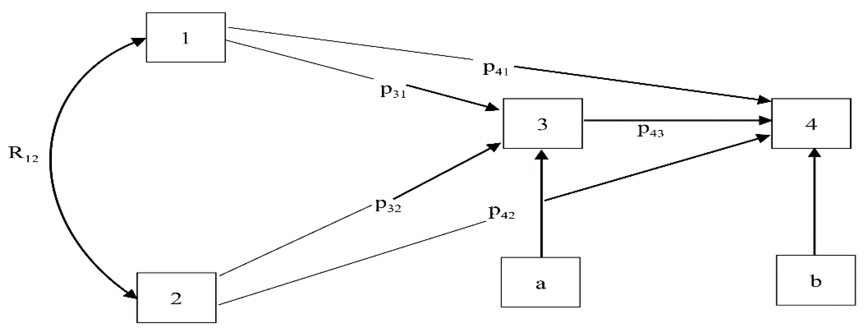
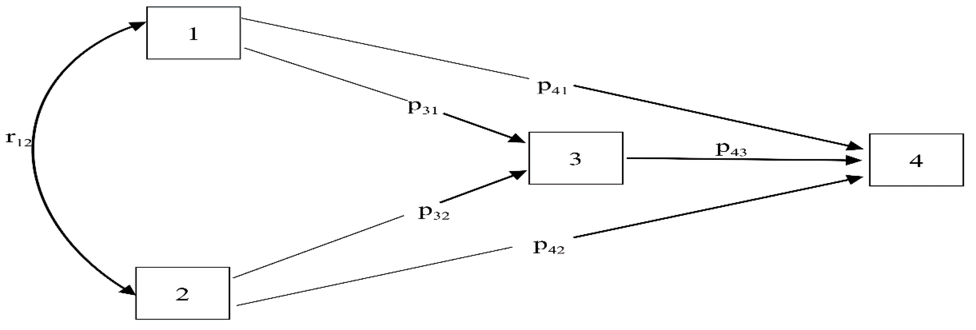
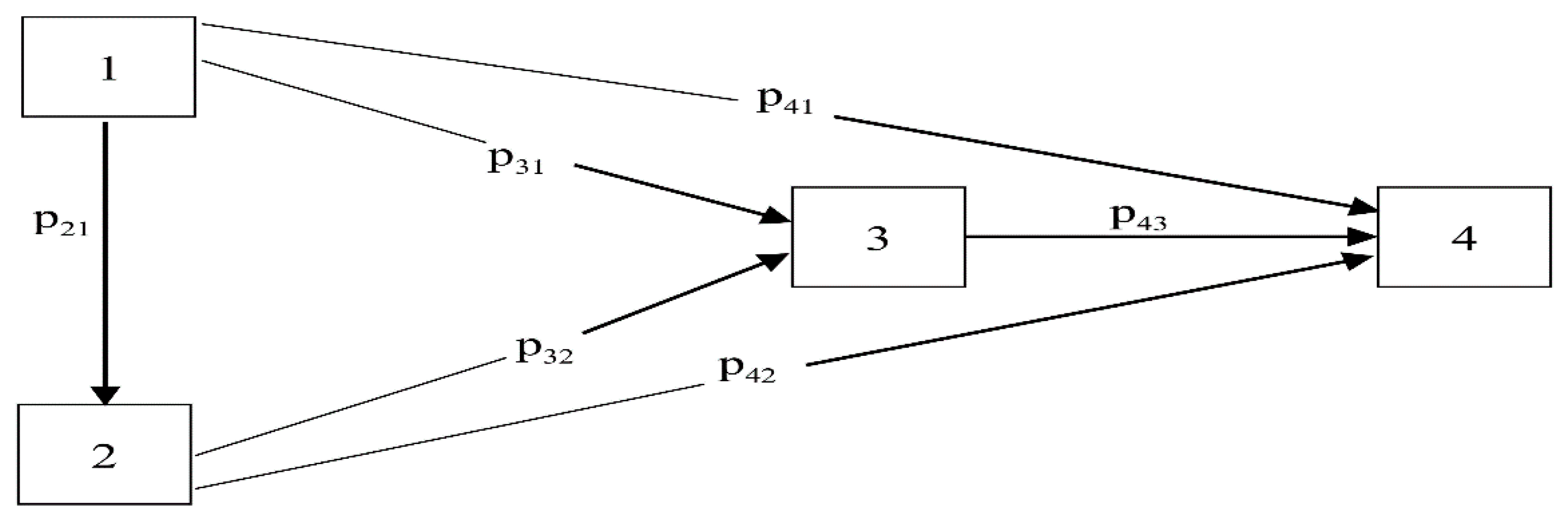
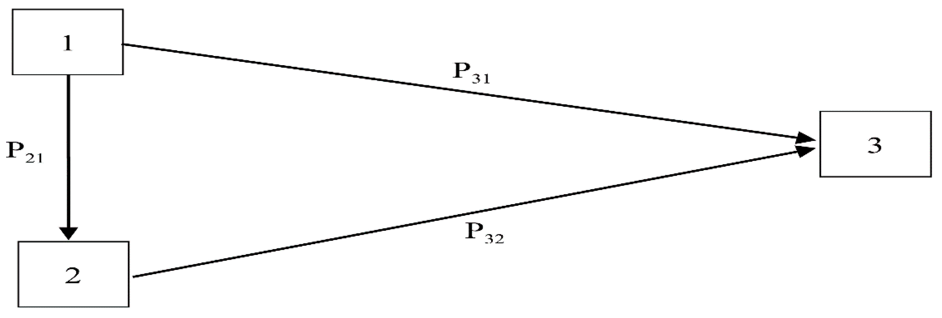
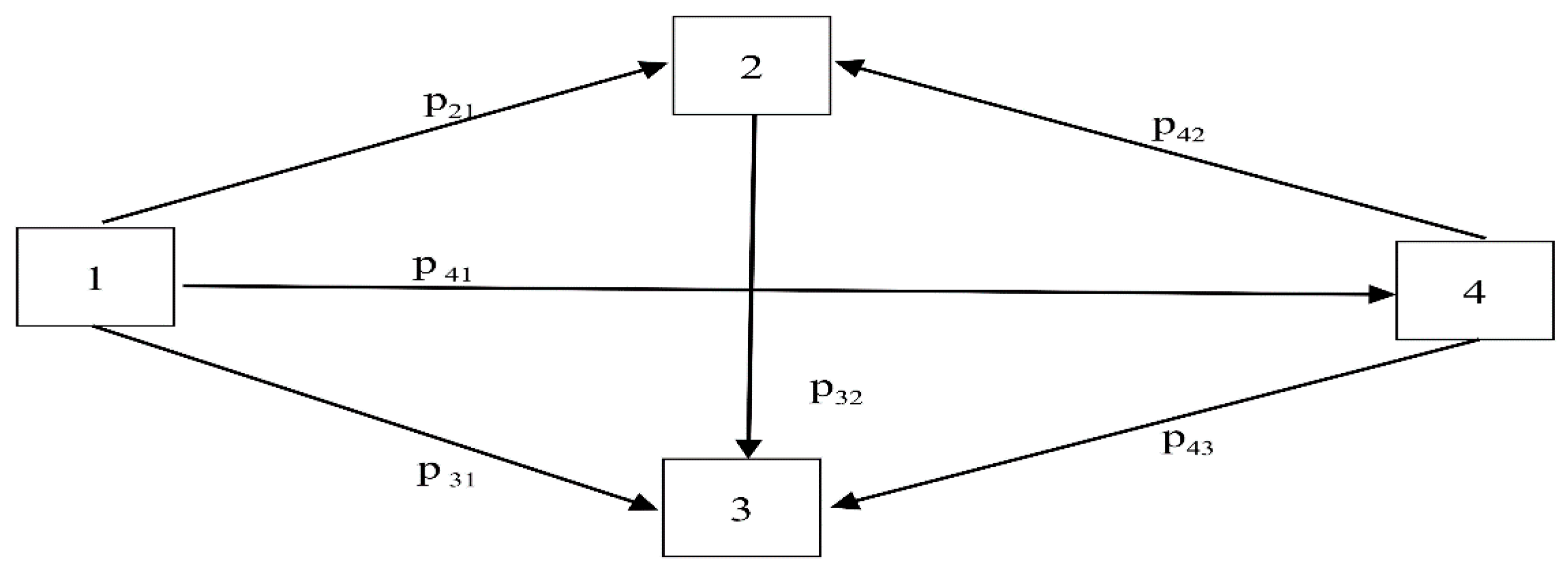
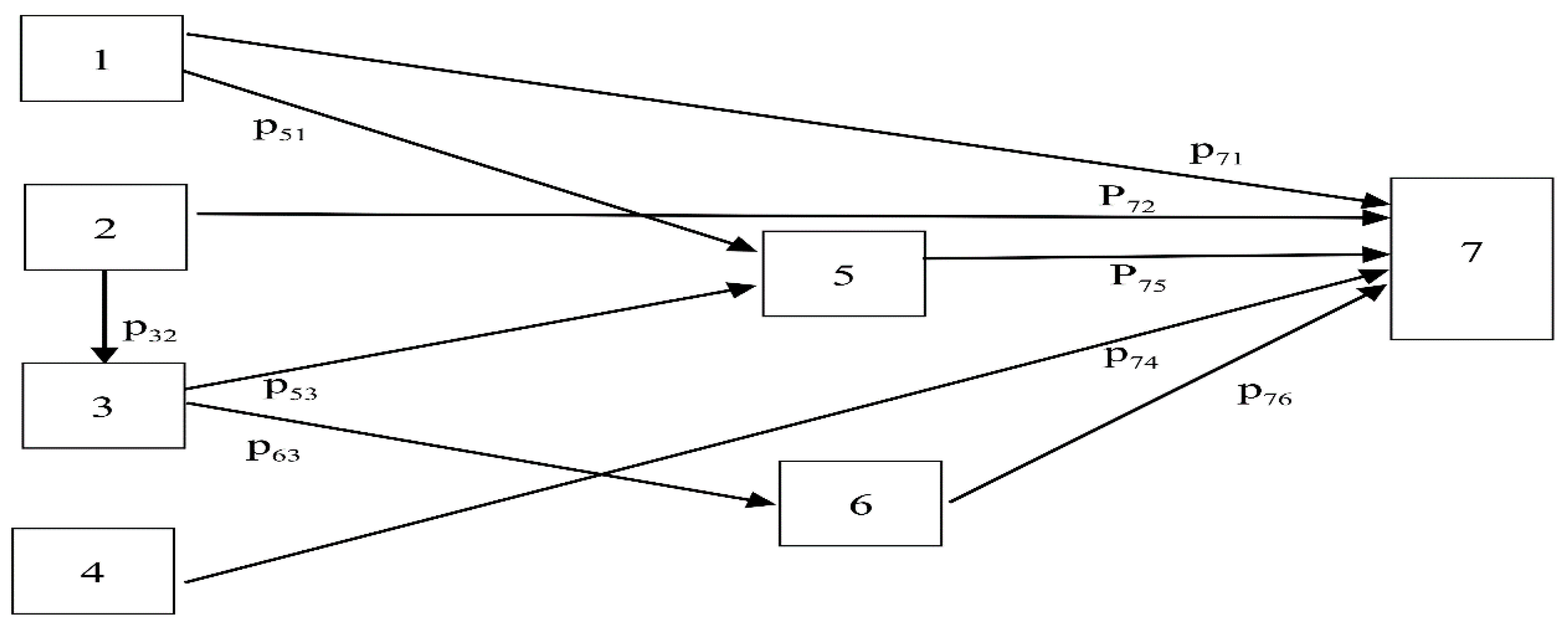
3.1. Path Analysis-GMM Model

The path analysis–GMM model is a specific analysis of regression analysis with the purpose of analyzing variables (both independent variables and dependent variables) to find out the direct or indirect correlation, in which the impact may be passing between each other or originate in both. Additionally, it analyzes whether there are any external factors that promote the relationship among variables as per the reason in theory. The reason for studying the path analysis–GMM model is to study the causal relationships between variables. Although correlation analysis—either simple correlation, partial correlation, multiple correlation, canonical correlation—or regression analysis can answer this question, it can deal with some limitations in some issues, especially in the correlation between variables, which is the objective of the path analysis–GMM model.

The process of the path analysis–GMM model is as follows:

• Draw path diagram or causal model

The path diagram is the most important part, and should be drawn first, because the path diagram describes the correlation among the variables. However, drawing the path analysis–GMM model is not something that we could do easily by ourselves. The path diagram is a model from a theory. As such, the path diagram must done according to theory. Once done, it is both a problem or hypothesis to be proven, and the objective at the same time. To prove the path, it must be done one at a time, as well as eliminate any unnecessary paths. To do so, it does not mean that the theory behind such paths is not realistic, but it does mean that there are sampling errors that contain unappropriated data to support such theory.

There are two types of variables in the path diagram: endogenous variables and exogenous variables. To understand the difference between these variables will result in drawing the path equation system correctly.

Exogenous variables are variables that can be varied because of external variables or variables that impact other variables within the path directly or indirectly where the exogenous variable itself has been impacted from another external influence.

Endogenous variables are the variables within the path diagram, and vary from the influence of exogenous variables or from the influence of the variables in the same path.

Assume that the theories confirm that variable numbers one, two, three, and four are related in the path as follows:

From Figure 1, variables one and two are exogenous variables, because the variation of both variables are from external factors of the path, or because variables one and two impact the other variables, which are variables three and four. Variables three and four are endogenous variables, because variable three is impacted from exogenous variables (variables one and two). Variable four is also an endogenous variable, because it is impacted from exogenous variables (variables one and two) and an endogenous variable in the same path (variable three) and from both exogenous variables one and two. Variables one and two are correlated and not separated as independent variables (so-called correlated causes). Please notice the arrow with two ends.

In addition, we can further analyze Figure 2 by looking at the path (arrow) to see:

- Variable three is directly impacted by variables three and two.

- Variable three is indirectly impacted by variable two through variable one, and is indirectly impacted by variable one through variable two.

- Variable four is directly impacted by variables one, two, and three.

- Variable four is indirectly impacted by variable one through variables two and three, and is indirectly impacted by variable two through variable one and three.

- a and b are residual.

Remark:

- $p_{ij}$ is the path coefficient to represent level (percentage). The influence of variable j’s impact on variable i such as $p_{31}$ shows the level of influence of variable one, which impacts variable three.

- $r_{ij}$ is the correlation of variable j and variable i.

- In fact, $p_{ij}$ is the population correlation of variable j and variable i, where $p_{ij}={\rho }_{ij}$, which can be easily proven.

For analyzing the path and to draw the path diagram, it is assumed as follows:

- The correlation of the path is unidirectional, or a one-way causal flow. Any variable at any time cannot be both the cause and effect of other variables at the same time. The arrow should run in the same direction, which is from left to right. It cannot be reversed from right to left (except for the exogenous variable, which can be a correlated cause of the endogenous variable).

- The correlation between variables is a causal linear additive model. It cannot be curvilinear, multiplicative, interactive, or others.

- The residual is free from the independent variable and dependent variable.

- The value of the variable is measured to be at the interval scale.

• Path equation and calculation of path coefficient

Normally, the path equation can be drawn using the basis of the path diagram, and then the equation can gradually draw to other paths, one path at a time, until all of the paths are completed. The variable that the arrow points at is a dependent variable, and all of the variables on the same path can be either exogenous variables or endogenous variables, or can both be independent variables. The equation will be arranged the same as the regression analysis by trying to reduce the quantity of equations to be as low as possible by combining the equations, showing the correlation of independent variables and the same dependent variable in the same equation. Any equation that needs to stay alone will be another equation. In general, the overall equations should not be more than all of the variables (variables in path diagram) [56,57].

When all of the equations are done and cover the relation in the path diagram, an analysis is performed to estimate the coefficient in each path (or each equation) by regression analysis. The result will be the path coefficient and estimated equation of the path equation. After that, if we want to know the quantity of the indirect influence of any variable, we substitute the estimated equation to the other equation to get the answer. The truth as indicated in the theory of whether such a path is necessary or not can be tested by proceeding in the same way as above, but only changing some path diagrams, as appropriate.

• Path Equation

Assume that all of the variables in the system $r+1$ are $X_1,X_2,\dots X_{r+1}$, where $\mathrm{E}\left(X_j\right)={\mu }_j$ and $V\left(X_j\right)={\sigma }_j^2;j=1\left(1\right)\left(r+1\right)$. Therefore, the path equation $k$; $k=1\left(1\right)\left(r+1\right)$ will be as follows:

$$X_{ki}={\beta }_0+{\beta }_1{X}_{ij}+{\beta }_2{X}_{2i}+\dots +{\beta }_r{X}_{ri}+u_i$$

(1)

Combining all of the values of i and dividing by N will derive the average value equation:

$${\mu }_k={\beta }_0+{\beta }_1{\mu }_1+{\beta }_2{\mu }_2+\dots +{\beta }_r{\mu }_r+{\mu }_u$$

(2)

Equations (1) and (2) will form a new equation as follows:

$$X_{ki}-{\mu }_{\mathrm{k}}={\beta }_1(X_{1i}-{\mu }_1)+{\beta }_2(X_{2i}-{\mu }_2)+\dots +{\beta }_r(X_{ri}-{\mu }_r)+u_i-u_u$$

(3)

To format Equation (3), divide all with ${\sigma }_k$ and multiply ${\beta }_j(X_{ji}-{\mu }_j)$ by $\frac{{\sigma }_j}{{\sigma }_j};j=1\left(1\right)r$; then, the equation of the standardized variable is as follows:

$$\begin{array}{c}\frac{X_{ki}-{\mu }_k}{{\sigma }_k}={\beta }_1\frac{{\sigma }_1}{{\sigma }_k}(\frac{X_{1i}-{\mu }_1}{{\sigma }_1})+{\beta }_2\frac{{\sigma }_2}{{\sigma }_k}(\frac{X_{2i}-{\mu }_2}{{\sigma }_2})+\dots {\beta }_r\frac{{\sigma }_r}{{\sigma }_k}(\frac{X_{ri}-{\mu }_r}{{\sigma }_r})\\ +\frac{{\sigma }_u}{{\sigma }_k}(\frac{u_i-{\mu }_u}{{\sigma }_u})\end{array}$$

(4)

Or:

$$Z_{ki}=({\beta }_1\frac{{\sigma }_1}{{\sigma }_k})z_{1i}+({\beta }_2\frac{{\sigma }_2}{{\sigma }_k})z_{2i}+\dots +({\beta }_r\frac{{\sigma }_i}{{\sigma }_k})z_{ri}+(\frac{{\sigma }_u}{{\sigma }_k})e_i$$

(5)

However, ${\rho }_{ki}={\beta }_j\frac{{\sigma }_i}{{\sigma }_k};j=1\left(1\right)r$ and ${\rho }_{ki}=p_{kj}$ is the path coefficient. To substitute the value in Equation (5), it will appear in the path equation at k as follows. Such an equation will be in a general form or specific form, which is composed of fewer independent variables than r.

$$Z_{ki}={\mathrm{p}}_{\mathrm{ki}}{z}_{1i}+p_{k2}{z}_{2i}+\dots +p_{kr}{z}_{ri}+p_{ku}{e}_i:k=1(1)r$$

(6)

It depends on why $z_k$ is varied, or what the causal factors are (see equation sample of path diagram).

From Equation (6), it can be noted that although e (e is residual) has coefficient $p_{ku}$, it is shown that in addition to the exogenous variable and endogenous variable influence on $z_k$ it is also residual, which is the unindicated factor in the path diagram, and also co-influences to impact on $z_k$. However, in theory, it is allowed that $\left(p_{ku}{e}_i\right)$ is the random variable, and the value of $p_{ku}$ can be estimated in Equation (7) as follows:

From Equation (6), it is found that:

$$\begin{array}{c}V(z_{ki})=V(p_{\mathrm{k}1}{z}_{1i}+p_{k2}{z}_{2i}+\dots +p_{kr}{z}_{r1}+p_{ku}{e}_i)\\ 1={\displaystyle \sum _{j=1}^{r}V}(p_{kj}{z}_{ji})+{\displaystyle \sum _{s\ne t}^r{p}_{ks}{p}_{kt}\mathrm{cov}(z_s{z}_t)+V(p_{ku}{e}_i)}\\ 1={\displaystyle \sum _{j=1}^r{p}_{kj}^2}+{\displaystyle \sum _{s\ne t}^r{r}_{st}}{p}_{ks}{p}_{kt}+p_{ku}^2\end{array}$$

(7)

The covariance = ${\displaystyle \sum _j^r}$ (direct influence of $z_j$ to $z_k$) + ${\displaystyle \sum _{s\ne t}^r}$ (indirect influence of independent variable) + other influence of $z_k$.

Please consider the following path diagram and draw an equation:

From Figure 2, it was found that in case $z_1$ and $z_2$ are correlated causes of $z_3$, we will not separate $z_1$ and $z_2$ from each other, but rather gather them in the form of co-variables that impact on $z_3$ (see the variable that the arrow runs into), which means that $z_3$ is impacted by $z_1$ and $z_2$ both directly and indirectly. $z_4$ is impacted directly by $z_3$ and is impacted both directly and indirectly by $z_1$ and $z_2$.

The equation of path diagram 1 is shown as follows:

$$Z_3=p_{31}{z}_1+p_{32}{z}_2+p_{3u}{z}_e$$

$$Z_4=p_{41}{z}_1+p_{42}{z}_2+p_{43}{z}_3+p_{4u}{z}_e$$

From Figure 3, it was found that in case $z_1$ is an exogenous variable while $z_2$, $z_3$, and $z_4$ are endogenous variables, therefore, the equation will be as follows (indicate the variable at the end of arrow as the dependent variable, and the variable at the front of arrow as the independent variable at any time of drawing an equation):

$$Z_1=p_{1u}e$$

$$Z_2=p_{21}{z}_1+p_{2u}e$$

$$Z_3=p_{31}{z}_1+p_{32}{z}_2+p_{3u}e$$

$$Z_4=p_{41}{z}_1+p_{42}{z}_2+p_{43}{z}_3+p_{4u}e$$

From Figure 4, it was found that in case $z_1$ is an exogenous variable, therefore, the path equation system is shown as follows:

$$Z_1=p_{1u}e$$

$$Z_2=p_{21}{z}_1+p_{2u}e$$

$$Z_3=p_{31}{z}_1+p_{32}{z}_2+p_{3u}e$$

From Figure 5, it was found that in case $z_1$ is an exogenous variable that impacts indirectly on $z_4$ through $z_2$ and $z_3$, therefore, the path equation system is shown as follows:

$$Z_1=p_{1u}e$$

$$Z_2=p_{21}{z}_1+p_{2u}e$$

$$Z_3=p_{31}{z}_1+p_{32}{z}_2+p_{3u}e$$

$$Z_4=p_{41}{z}_1+p_{42}{z}_2+p_{43}{z}_3+p_{4u}e$$

From Figure 6, it was found that in case $z_1$ and $z_2$ are exogenous variables, the path equation is shown as follows:

$$Z_1=p_{1u}e$$

$$Z_2=p_{2u}e$$

$$Z_3=p_{31}{z}_1+p_{32}{z}_2+p_{3u}e$$

$$Z_4=p_{41}{z}_1+p_{42}{z}_2+p_{43}{z}_3+p_{4u}e$$

$$Z_5=p_{51}{z}_1+p_{52}{z}_2+p_{53}{z}_3+p_{54}{z}_4+p_{5u}e$$

From Figure 7, it was found that in case $z_1$, $z_2$, and $z_4$ are exogenous variables, the path equation is shown as follows:

$$Z_1=p_{1u}e$$

$$Z_2=p_{2u}e$$

$$Z_3=p_{32}{z}_2+p_{3u}e$$

$$Z_4=p_{4u}e$$

$$Z_5=p_{51}{z}_1+p_{53}{z}_3+p_{5u}e$$

$$Z_6=p_{63}{z}_3+p_{6u}e$$

$$Z_7=p_{71}{z}_1+p_{72}{z}_2+p_{74}{z}_4+p_{75}{z}_5+p_{76}{z}_6+p_{7u}e$$

For parameter estimation, the researcher applied the GMM model, which can be described as follows:

The generalized method of moments (GMM) is the direct estimation of parameter value from moment conditions that are put into the model. These moment conditions can be linear attributes in the parameter; however, they often become nonlinear. In order to find out the parameter, the number of moment conditions should be at least equal to the number of unknown parameters.

In case the moment conditions are nonlinear, the instrument that is used to estimate the variables is called the instrumental variables estimator.

The generalized method of moments (GMM) [51,52] is the model that is a set of R, where the moment conditions will be as follows:

$$E\left\{f\left(w_t,z_t,\theta \right)\right\}=0$$

(8)

where $f$ = the vector function that is composed of elements R. $0$= the dimension vector, which is equal to K, and is the vector of all of the unknown parameters. $W_1$ = the vector of variables, which is the observable variable, and can be either endogenous variables or exogenous variables. Meanwhile, $Z_1$ = is the vector of instruments.

From the example above, $w_t^{\prime }=\left(C_{t+1}/C_t.r_{t+1}\right)$ .

In the estimation of $\theta$, the same method as above by using the equivalent sample with Equation (8) is defined by:

$$g_r(\theta )=\frac{1}{T}{\displaystyle \sum _{t=1}^{r}f(w_t,z_t.\theta )}$$

(9)

If the moment that conditions that are equal to R are equivalent to the unknown parameter K, we can have elements in Equation (9) that are equal to 0 and find out θ, which will obtain a unique consistent estimator as follows:

If $f$ is nonlinear in $\theta$, a solution may not exist.

If the moment conditions are less than the parameters, uniquely unknown parameters cannot be found by using Equation (9), which is equal to 0.

The selection of the estimator for θ is in the form where the vector of sample moments has a value that is close to 0, meaning that the quadratic form in $g_r(\theta )$ has the lowest value as follows:

$$\underset{\theta }{\min }{\mathrm{Q}}_{\mathrm{r}}(\theta )=\underset{\theta }{\min }{\mathrm{g}}_{\mathrm{r}}{(\theta )}^{\prime }{W}_r{\mathrm{g}}_{\mathrm{r}}(\theta )$$

(10)

where $W_r$ is the positive definite matrix with $p$ lim $W_r=W$. The solution of this problem is the generalized method of moments or GMM estimator $\theta$. It can be presented that the GMM estimator has consistent and normal linear distribution under weak regularity conditions.

In practice, the GMM estimator is derived from minimizing Equation (10).

It is known that a different matrix to weight $W_r$ will also have different consistent estimators by linear co-variance. The appropriately weighted matrix will derive the least variation for the GMM estimator, which is the inverse of the covariance of sample moments. In case there is no autocorrelation, the appropriated weighted matrix can be written as follows:

$$W^{OPT}={\left(\mathrm{E}\left\{\mathrm{f}\left({\mathrm{w}}_{\mathrm{t}},z_t,\theta \right)f{\left(w_t,z_1,\theta \right)}^{\prime }\right\}\right)}^{-1}$$

In general, the matrix will depend on the vector of unknown parameter θ, which cannot be found in the linear model. The solution involves many estimation processes, starting from the first one using the suboptimal choice of $W_r$, which is not dependent on θ, such as the identity matrix to find the first consistent estimator. Assuming that ${\widehat{\theta }}_{[1]}$, after that, we will estimate the appropriated weighted matrix by:

$$W_r^{OPT}={\left(\frac{1}{n}{\displaystyle \sum _{t=1}^{T}f}\left({\mathrm{w}}_{\mathrm{t}},z_t{\widehat{\theta }}_{[1]}\right)\mathrm{f}{\left({\mathrm{w}}_{\mathrm{t}},z_t,{\widehat{\theta }}_{[1]}\right)}^{\prime }\right)}^{-1}$$

(11)

The second process is to find an efficient asymptotic GMM estimator, ${\widehat{\theta }}_{GMM}$, by the asymptotic distribution as follows:

$$\sqrt{T}\left({\widehat{\theta }}_{GMM}-\theta \right)\to N(o,v)$$

(12)

where the asymptotic covariance matrix $V$ is:

$$V={\left({\mathrm{D}\mathrm{W}}^{\mathrm{OPT}}{\mathrm{D}}^{\prime }\right)}^{-1}$$

(13)

where $D=K\times$ derivative matrix R:

$$D=\mathrm{E}\left\{\frac{\partial {\mathrm{f}(\mathrm{w}}_{\mathrm{t}},z_t,\theta )}{\partial {\theta }^{\prime }}\right\}$$

(14)

For the over-identifying restrictions test of nonlinear models, if the moment conditions have been correctly defined, the test statistic will be:

$$\zeta ={\mathrm{Tg}}_{\mathrm{T}}{\left({\widehat{\theta }}_{GMM}\right)}^{\prime }{\mathrm{W}}_{\mathrm{T}}^{\mathrm{OPT}}{\mathrm{g}}_{\mathrm{t}}\left({\widehat{\theta }}_{GMM}\right)$$

(15)

where ${\widehat{\theta }}_{GMM}$ is the appropriated GMM estimator, and $W_T^{OPT}$ is the appropriated weighted matrix in Equation (11); and ζ has a chi square asymptotic distribution by R–K degrees of freedom. In the case that it is exactly identified, the degrees of freedom will be 0, and then, there is nothing to test.

3.2. Measurement of the Forecasting Performance

In this research, we decided to use the MAPE and RMSE values to compare the forecasting accuracy in each model. The calculation equations are shown as follows [62,63]:

$$MAPE=\frac{1}{n}{\displaystyle \sum _{i=1}^n\left|\frac{{\widehat{y}}_i-y_i}{y_i}\right|}$$

(14)

$$RMSE=\sqrt{\frac{1}{n}{\displaystyle \sum _{i=1}^n{\left({\widehat{y}}_i-y_i\right)}^2}}$$

(15)

Based on a review of the previous research, a number of studies differed in the used models for the analysis, research process, and duration. In this paper, we adapted the path analysis–GMM model to produce the best result, yet it was also applicable for optimization in strategy planning to achieve sustainability. To construct the model, the authors have applied a path analysis model integrated with the GMM model to close the gaps in and eliminate the weaknesses of each model, especially the past models, which required estimations of parameter values by using the ordinary least squares (OLS) method, which can produce more spurious results. Therefore, the authors are of the belief that the path analysis–GMM model results in increased accuracy and will be more appropriate for future policy planning and research direction. This path analysis–GMM model differs from previous models, and is not similar to any of the other currently existing models. The research process can be demonstrated as follows.

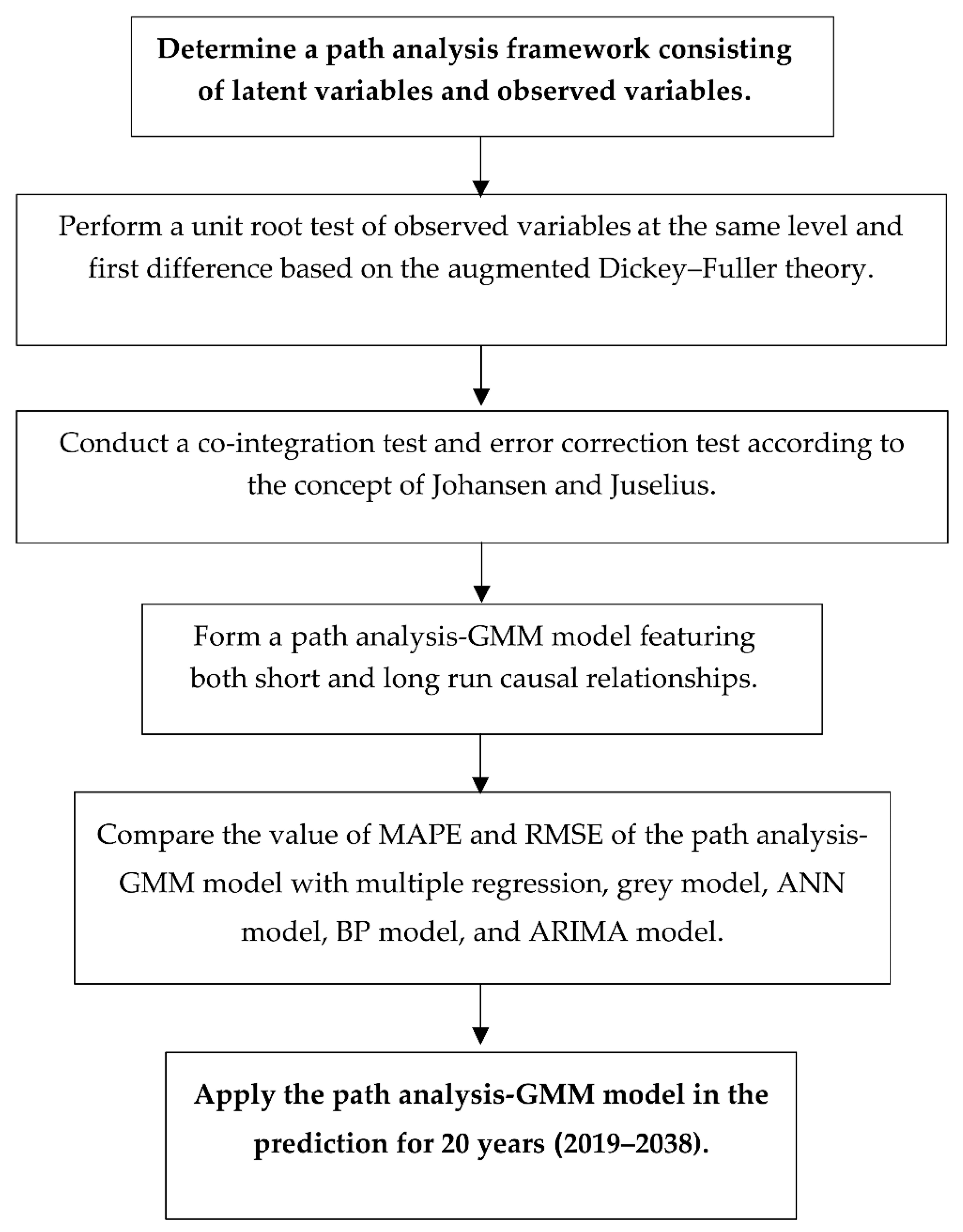
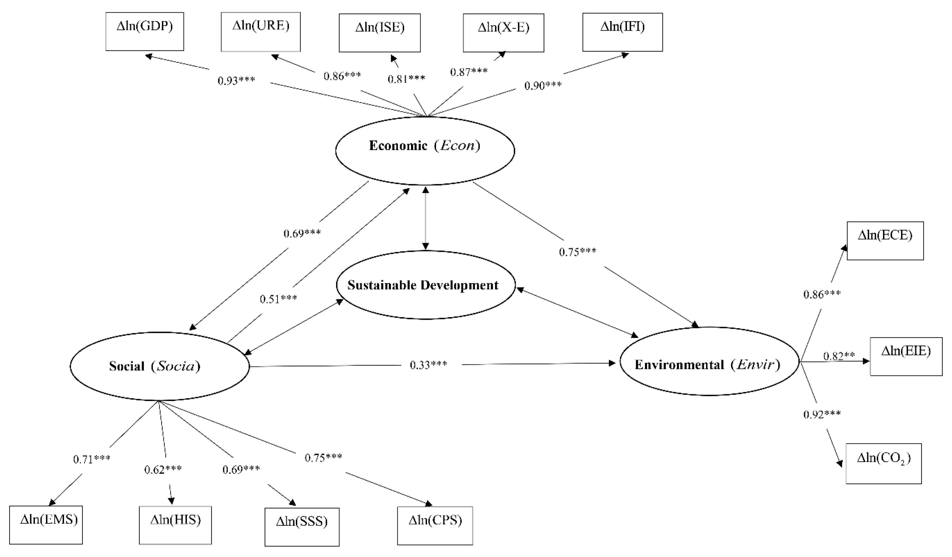
• Determine a variable framework based on the path analysis [56,57], which contains both latent variables (economic $(Econ)$, social $(Socia)$, and environmental $(Envir)$, while the observed variables contained 12 factors that are economic indicators; these are per capita GDP $(GDP)$, urbanization rate $(URE)$, industrial structure $(ISE)$, net exports $(X-E)$, and indirect foreign investment $(IFI)$. The authors have found the data regarding these economical indicators from the Office of the National Economic and Social Development Board (NESDB) and National Statistic Office Ministry of Information and Communication Technology. For the social indicators, which are employment $(EMS)$, health and illness $(HIS)$, social security $(SSS)$, and consumer protection $(CPS)$, the authors found the data from the Office of the National Economic and Social Development Board (NESDB) and the National Statistic Office Ministry of Information and Communication Technology. For the environmental indicators, which are energy consumption $(ECE)$, energy intensity $(EIE)$, and carbon dioxide emissions $(C{O}_2)$, the authors found the data from the Department of Alternative Energy Development and Efficiency.
• Perform a unit root test of the observed variables according to the concept of the augmented Dickey–Fuller test [58], and analyze a long-term causal relationship by using the theory of Johansen Juselius [59,60,61].
• Take the co-integrated variables at the same level to build a path analysis–GMM model, which features both short-term and long-term causal relationships, adding to the presentation of direct and indirect effects [61].
• Assess a best linear unbiased estimation (BLUE) feature of the path analysis–GMM model, and test its goodness of fit [62,63].
• Compare the effectiveness of the path analysis–GMM model with other models, including multiple regression, the grey model, ANN model, back propagation neural network (BP) model, and ARIMA model through a performance measure of MAPE and RMSE.
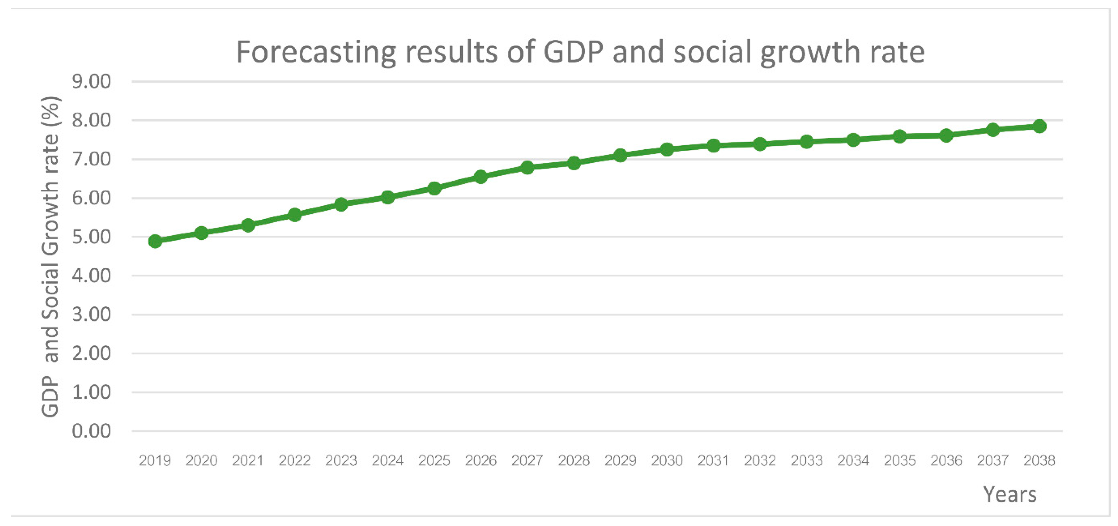
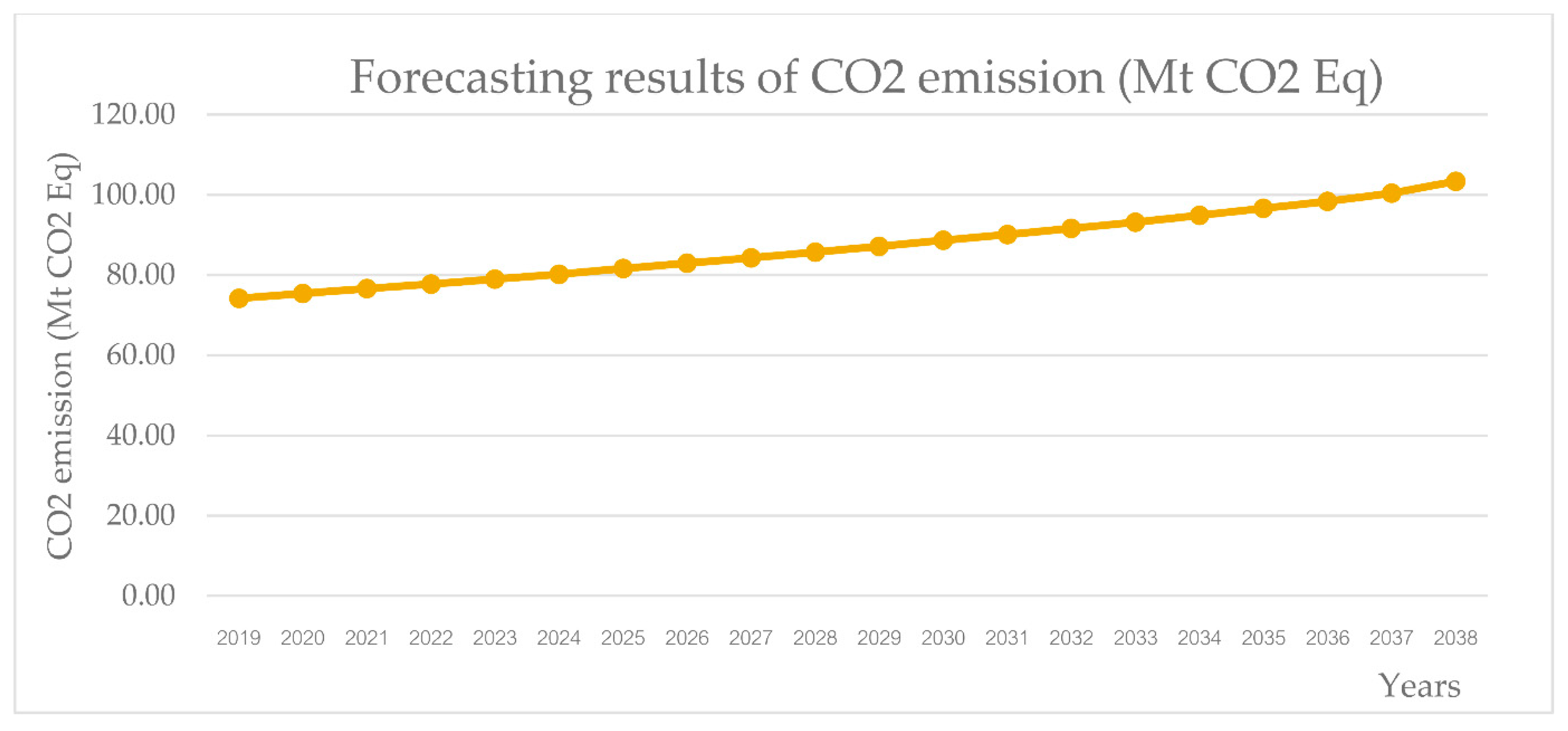
• Forecast the future economic growth and CO₂ emissions by using the path analysis–GMM model from 2019 to 2038, totaling 20 years. The flowchart of the path analysis–GMM model is shown in Figure 8.

4. Empirical Analysis

4.1. Screening of Influencing Factors for Model Input

In this paper, the path analysis framework was determined. There were three factors of the latent variables, namely, economic $(Econ)$, social $(Socia)$, and environmental $(Envir)$, while the observed variables contained 12 factors including per capita gross domestic product $(GDP)$, urbanization rate $(URE)$, industrial structure $(ISE)$, net exports $(X-E)$, indirect foreign investment $(IFI)$, employment $(EMS)$, health and illness $(HIS)$, social security $(SSS)$, consumer protection $(CPS)$, energy consumption $(ECE)$, energy intensity $(EIE)$, and carbon dioxide emissions $(C{O}_2)$. As for the correlation test, the factors will be undergone for R Pearson correlation coefficient of sustainable development dimension’s indicators before constructing the path analysis–GMM model, as illustrated in

Table 1. R Pearson correlation coefficient of sustainable development dimension’s indicators.

$\mathbf{Dimensions}\mathbf{of}\mathbf{Sustainable}\mathbf{Development}({\mathit{X}}_{\mathit{i}})$	Parameters	$\mathbf{Dimensions}\mathbf{of}\mathbf{Sustainable}\mathbf{Development}({\mathit{Y}}_{\mathit{i}})$
		$\mathbf{Economic}(\mathit{E}\mathit{c}\mathit{o}\mathit{n})$	$\mathbf{Social}(\mathit{S}\mathit{o}\mathit{c}\mathit{i}\mathit{a})$	$\mathbf{Environmental}(\mathit{E}\mathit{n}\mathit{v}\mathit{i}\mathit{r})$
Economic $(Econ)$	$r(X,Y)$	1	0.73 ***	–0.61 ***
	p-value	-	0.00	0.00
Social $(Socia)$	$r(X,Y)$	0.49 ***	1	–0.65 ***
	p-value	0.00	-	0.00
Environmental $(Envir)$	$r(X,Y)$	–0.67 ***	−0.51 ***	1
	p-value	0.00	0.00	-

*** denotes significance $\alpha =0.01$.

.

Table 1 is the analysis of the R Pearson correlation coefficient of the sustainable development dimension’s indicators. The results from the above analysis show that every factor has a significant relationship at the stated significance level, $\alpha =0.01$. The economic factors $(Econ)$ are relative to the social factors $(Socia)$ with a positive relationship trend, while the economic factors $(Econ)$ are relative to the environmental $(Envir)$ factors in a negative direction. The above findings show that all of the factors are relative to each other, and that is appropriate for further application in the model construction.

In structuring a framework of the path analysis model, the stationary observed variables at level I (0) or the first level I (1) must be identified and selected. This can be done with the application of the unit root test based on the augmented Dickey–Fuller theory. In this paper, only the stationary observed variables at the same level were taken. Here, the study found that the 12 causal factors were stationary at the first difference I (1), as illustrated in

Table 2. Unit root test at first difference I (1).

Tau Test		MacKinnon Critical Value
Variables	Value	1%	5%	10%
$\mathsf{\Delta }\ln \left(\mathrm{GDP}\right)$	−5.99 ***	−4.25	−3.05	−2.70
$\mathsf{\Delta }\ln (\mathrm{URE})$	−5.51 ***	−4.25	−3.05	−2.70
$\mathsf{\Delta }\ln \left(\mathrm{ISE}\right)$	−4.95 ***	−4.25	−3.05	−2.70
$\mathsf{\Delta }\ln (\mathrm{X}-\mathrm{E})$	−4.05 ***	−4.25	−3.05	−2.70
$\mathsf{\Delta }\ln \left(\mathrm{IFI}\right)$	−5.21 ***	−4.25	−3.05	−2.70
$\mathsf{\Delta }\ln \left(\mathrm{EMS}\right)$	−4.75 ***	−4.25	−3.05	−2.70
$\mathsf{\Delta }\ln \left(\mathrm{HIS}\right)$	−4.31 ***	−4.25	−3.05	−2.70
$\mathsf{\Delta }\ln \left(\mathrm{SSS}\right)$	−4.29 ***	−4.25	−3.05	−2.70
$\mathsf{\Delta }\ln \left(\mathrm{CPS}\right)$	−4.67 ***	−4.25	−3.05	−2.70
$\mathsf{\Delta }\ln \left(\mathrm{ECE}\right)$	−6.55 ***	−4.25	−3.05	−2.70
$\mathsf{\Delta }\ln \left(\mathrm{EIE}\right)$	−4.90 ***	−4.25	−3.05	−2.70
$\mathsf{\Delta }\ln (\mathrm{C}{\mathrm{O}}_2)$	−6.07 ***	−4.25	−3.05	−2.70

Note: $GDP$ is the per capita GDP, $URE$ is the urbanization rate, $ISE$ is the industrial structure, $X-E$ is the net exports, $IFI$ is the indirect foreign investment, $(EMS)$ is the employment, $(HIS)$ is the health and illness, $(SSS)$ is the social security, $(CPS)$ is the consumer protection, $ECE$ is the energy consumption, $EIE$ is the energy intensity, and $C{O}_2$ is the carbon dioxide emissions. *** denotes a significance, $\alpha$ = 0.01, compared to the Tau test with the MacKinnon critical value, $\mathsf{\Delta }$ is the first difference, and $\ln$ is the natural logarithm.

.

Table 2 shows that all of the factors were non-stationary at Level I (0). Therefore, the first difference was required, and all of the factors were found to be stationary at Level I (1). This indicates that the value of the Tau test was greater than the MacKinnon critical value, signifying that every factor was significant at 1%, 5%, and 10%. Thus, it was suitable to use them for the co-integration test proposed by Johansen and Juselius, as shown in

Table 3. Co-integration test by Johansen and Juselius.

Variables	Hypothesized No of CE(S)	Trace Statistic Test	Max-Eigen Statistic Test	MacKinnon Critical Value
				1%	5%
$\mathsf{\Delta }\ln \left(\mathrm{GDP}\right)$, $\mathsf{\Delta }\ln (\mathrm{URE})$, $\mathsf{\Delta }\ln \left(\mathrm{ISE}\right)$, $\mathsf{\Delta }\ln (\mathrm{X}-\mathrm{E})$, $\mathsf{\Delta }\ln \left(\mathrm{IFI}\right)$, $\mathsf{\Delta }\ln \left(\mathrm{EMS}\right)$, $\mathsf{\Delta }\ln \left(\mathrm{HIS}\right)$, $\mathsf{\Delta }\ln \left(\mathrm{SSS}\right)$, $\mathsf{\Delta }\ln \left(\mathrm{CPS}\right)$, $\mathsf{\Delta }\ln \left(\mathrm{ECE}\right)$, $\mathsf{\Delta }\ln \left(\mathrm{EIE}\right)$, $\mathsf{\Delta }\ln (\mathrm{C}{\mathrm{O}}_2)$	None **	210.50 **	235.05 **	15.75	12.50
	At Most 1 **	75.95 **	94.60 **	7.50	5.55

** denotes significance α = 0.01.

.

4.2. Analysis of Co-Integration

According to Table 3, the outcomes showed that all observed variables had a significant level at 1% and 5% because the trace values were 210.50 and 75.95, which were higher than the MacKinnon critical values. In addition, the maximum eigenvalue test results were 235.05 and 94.60, which were higher than the MacKinnon critical values. Hence, this indicates that all variables are suitable for the modeling of a path analysis-GMM model.

4.3. Formation of Analysis Modeling with the Path Analysis-GMM Model

The path analysis-GMM model is built upon a short- and long-term causal relationship, where the study showed that such a relationship of latent variables had a direct causal, and indirect effect. This can be illustrated further in Figure 9. In fact, the path analysis-GMM model was tested and qualified for a BLUE feature.

Figure 9 demonstrates the analysis of the casual relationship in the path analysis–GMM model, where the latent variables are economic $(Econ)$, social $(Socia)$, and environmental $(Envir)$, while the observed variables consist of per capita GDP $(GDP)$, urbanization rate $(URE)$, industrial structure $(ISE)$, net exports $(X-E)$, indirect foreign investment $(IFI)$, employment $(EMS)$, health and illness $(HIS)$, social security $(SSS)$, consumer protection $(CPS)$, energy consumption $(ECE)$, energy intensity $(EIE)$, carbon dioxide emissions $(C{O}_2)$, and $EC{M}_{t-1}$. From the study, it provides a finding of which factors had direct effects, causal effects, and indirect effects, where the results can be seen in

Table 4. Results of relationship size analysis of the path analysis–GMM model.

Dependent Variables	Type of Effect	Independent Variables
		$\mathbf{Economic}(\mathit{E}\mathit{c}\mathit{o}\mathit{n})$	$\mathbf{Social}(\mathit{S}\mathit{o}\mathit{c}\mathit{i}\mathit{a})$	$\mathbf{Environmental}(\mathit{E}\mathit{n}\mathit{v}\mathit{i}\mathit{r})$	$\mathbf{Error}\mathbf{Correction}\mathbf{Mechanism}(\mathit{E}\mathit{C}{\mathit{M}}_{\mathit{t}-1})$
Economic $(Econ)$	DE	-	0.51 ***	-	−0.62 ***
	IE	-	-	-	-
Social $(Socia)$	DE	0.69 ***	-	-	−0.55 ***
	IE	-	-	-	-
Environmental $(Envir)$	DE	0.75 ***	0.33 ***	-	−0.04 **
	IE	0.21 ***	0.27 ***	-	-

Note: In the above, *** denotes significance $\alpha$ = 0.01, ** denotes significance α = 0.05, ${\chi }^2/df$ is 1.10, root mean square of error approximation ($RMSEA$) is 0.03, root mean squared residual ($RMR$) is 0.005, goodness of fit index ($GFI$) is 0.97, adjusted goodness of fit index ($AGFI$) is 0.95, R-squared is 0.95, the F-statistic is 121.00 (probability is 0.00), the Autoregressive Condition Heteroscedastic test (ARCH test) is 25.75 (probability is 0.1), the Lagrange multiplier test (LM test) is 1.27 (probability is 0.10), DE is the direct effect, and IE is the indirect effect.

.

Table 4 illustrates the parameters of the path analysis–GMM model at the statistically significant levels of 1% and 5%. With the analyzed findings, the path analysis–GMM model was deemed to be ideal due to its qualification of goodness of fit, where the values of RMSEA and RMR reached 0, while the GFI and AGFI values approached 1. Furthermore, when the model was tested for a BLUE feature, the result was positive, indicating that the path analysis–GMM model was an appropriate model to analyze the magnitude of the relationship. In addition, the problems of heteroskedasticity, multicollinearity, and autocorrelation were not found. Furthermore, the R-square value was equal to 95%, and the F-test value was greater than the F-critical value at a significance level of 1%. Therefore, the path analysis–GMM model can be used to analyze the magnitude of the relationship to the sustainable development policy. In detail, $(Econ)$ had a direct effect on, which was equivalent to 69% at a significance level of 1%. This indicates that when $(Econ)$ changed by about 1%, it affected $(Socia)$ by 69%. Meanwhile, the change in $(Socia)$ had a direct effect on $(Econ)$, which was equivalent to 51% at a significance level of 1%. This implies that when $(Socia)$ changes by about 1%, the variable $(Econ)$ will change by about 51%. Furthermore, the study showed that the relationship between $(Econ)$ and $(Socia)$ was a causal relationship. This type of relationship between $(Econ)$ and $(Socia)$ can also be called a cause-and-effect relationship.

In addition to this, $(Econ)$ was found to have a direct effect on $(Envir)$, which was equivalent to 75% at a significance level of 1%, implying that when $(Econ)$ changed by about 1%, it would affect $(Envir)$, which changed up to 75%. In terms of $(Econ)$, it had an indirect effect on $(Envir)$, which was equivalent to 21% at a significance level of 1%. This explains that when $(Econ)$ changed by about 1%, it influenced $(Envir)$ to change up to 21%, which is made transferable through $(Socia)$.

As for $(Socia)$, it had a direct effect on $(Envir)$ of about 33% at a significance level of 1%, which tells us that when $(Socia)$ makes a change of about 1%, it will make a change in $(Envir)$ of about 33%. Whereas $(Socia)$ was observed to have an indirect effect on $(Envir)$ of about 27% at a significance level of 1%, implying that when $(Socia)$ changed by about 1%, it would change $(Envir)$ up to 27%, which is made transferable through $(Econ)$.

In the case of ${\mathrm{ECM}}_{\mathrm{t}-1}$, it had a direct effect on $(Econ)$, where the parameter value was –0.62 at a significance level of 1%. This indicates that the adjustment rate of $(Econ)$ in the path analysis–GMM model toward equilibrium was 62%. In another case, ${\mathrm{ECM}}_{\mathrm{t}-1}$ had a direct effect on $(Socia)$, whose parameter value was –0.55 at a significance level of 1%. This implies that the adjustment rate of $(Socia)$ in the path analysis–GMM model toward equilibrium was 55%. In addition to ${\mathrm{ECM}}_{\mathrm{t}-1}$, it also had a direct effect on $(Envir)$, whose parameter value was –0.04 at a significance level of 5%. This explains that the adjustment rate of $(Envir)$ in the path analysis–GMM model toward equilibrium was 4%.

In the path analysis–GMM model, there was a comparison of model effectiveness by using the MAPE and RMSE. The mentioned values were taken to compare the same value types of other studied models consisting of multiple regression, the grey model, ANN model, BP model, and ARIMA model, as illustrated below.

Table 5. The performance monitoring of the forecasting models. ARIMA: autoregressive integrated moving average model, ANN: artificial neural natural model, BP: back propagation neural network, MAPE: mean absolute percentage error, RMSE: root mean square error.

Forecasting Model	MAPE (%)	RMSE (%)
Multiple Regression model	18.99	23.07
Grey model	14.09	15.26
ANN model	12.05	14.09
BP model	9.01	8.87
ARIMA model	5.11	4.39
Path analysis–GMM model	1.01	1.25

expresses the path analysis–GMM model with the lowest values of MAPE and RMSE, which were equivalent to 1.01% and 1.25%, respectively. The next textual lines elaborate a comparison between these two values with the same value types in other models. By looking at the ARIMA model, its MAPE and RMSE were 5.11% and 4.39%, respectively, while the BP model generated MAPE and RMSE with values of 9.01% and 8.87%, respectively. In the ANN model, the MAPE and RMSE were 12.05% and 14.09%, respectively, whereas the grey model produced values of MAPE and RMSE at 14.09% and 15.26%, respectively. Finally, the multiple regression model provided MAPE and RMSE values of 18.99% and 23.07%, respectively. Compared to those values, the path analysis–GMM model stands to be right and suitable for future forecasting.

4.4. A Forecasting Model on the Changes of Economic and Social Growth and CO₂ Emissions Based on the Path Analysis–GMM Model

Here, we applied the path analysis–GMM model to forecast the changes of both economic and social growth as well as CO₂ emissions from the energy consumption over the next 20 years (2019–2038), as illustrated in Figure 10 and Figure 11.

Figure 10 shows that economic and social growth in the next 20 years, ranging from 2019 to 2038, is most likely to increase with a growth rate of 7.85% (2038/2019). This demonstrates that Thailand has the capacity to develop its economy and society to achieve the national goals set by the government from 2019 to 2038.

Figure 11 shows that the CO₂ emissions in 20 years, from 2019 to 2038, in Thailand will increase at a growth rate of 39.37% (2038/2019) or 103.37 Mt CO₂ eq. by 2038. This shows that greenhouse gases emission will tends to increase gradually from 2019 to 2038.

5. Conclusions and Discussion

In the past, the implementation outcomes of the development policy for sustainability in the form of economic, social, and environmental growth since 1990 until the present were not satisfactory. This reflects the inefficiency of the national management, despite the economy growing and society improving. The sad fact is that the environment is being devastated as the other two aspects are growing. This is unacceptable, yet the same aspect regarding the environment has the potential for a negative effect in the future. In order to reduce this negative consequence, this study’s model is introduced as a policy-making tool for Thailand to support in its national management and policy making, as so to achieve the goal of sustainability.

With all of the research processes in place, this paper has achieved tremendous outcomes; developing the path analysis–GMM model is one of the research results. The above model presents the relationship of latent variables in three aspects: economic, social, and environmental. Each aspect has its own observed variables. The observed variables in the economy include per capita GDP urbanization (GDP), rate (URE), industrial structure (ISE), net exports (IFI), and indirect foreign investment (X-E), while the observed variables in society are related to employment (EMS), health and illness (HIS), social security (SSS), and customer protection (CPS). In the environmental aspect, energy consumption (EIE), energy intensity (ECE), and carbon dioxide emissions are the observed variables. From this study, it indicates that the economic, social, and environmental factors are directly and indirectly related, yet are causal. Here, the latent variables in each factor were correlated and influential over one another, enabling them to support national policy formulation in order to achieve future sustainable development. The path analysis model–GMM model had a goodness of fit feature, fulfilling all of the criteria. Additionally, it was identified to be a BLUE, which indicates its appropriate future application for long-term forecasting. In particular, this model differs from other existing models, as it outperforms at its highest effectiveness with the lowest value of MAPE and RMSE when compared to the original models, including the ARIMA model, BP model, ANN model, grey model, and multiple regression, respectively. However, when the model was used to forecast the economic and social growth during the period of 2019 to 2038, they were found to rise with a growth of 7.85% (2038), which goes as projected and targeted by the government from the past to the present (1990–2038). However, when the path analysis–GMM model was used to forecast the CO₂ emissions of the energy consumption in Thailand from 2019 to 2038, it was found that CO₂ emissions kept rising, and did not satisfy the government plans. This implies that Thailand failed to achieve sustainable development from 1990 to 2038, although Thailand has made national management strategies. Therefore, those in charge of policies and governance must emphasize this in the policy planning, and revise current policies in order to achieve national sustainability. In fact, such action is urgent, because the environmental recovery is slowing. This is supported by this study, where the results produced a parameter of ${\mathrm{ECM}}_{\mathrm{t}-1}$ of only about 4%, which shows a slow environmental adjustment toward the equilibrium. Such a percentage was lower than the adjustment rate of the economic and social balance, respectively. If the Thai government does not prioritize this and make it urgent, it will worsen the environmental damage more than ever, and make the issue more complex. In the meantime, a sustainability plan will not be materialized in the future.

Based on previous relevant studies, we distinguished this research with other past research studies. In this paper, we established the path analysis–GMM model by adapting the concept and theory of path analysis in the causality analysis. At the same time, the estimation of the parameter was done by using a GMM model. In fact, the software of linear structural relations (LISREL) was deployed along with Econometric Views (EVIEWS). Thus, such a model became a suitable and effective model for long-term forecasting when compared to other models. In addition, the model was a BLUE model by ensuring that there were no problems of heteroskedasticity, multicollinearity, and autocorrelation. This makes the model useful to expend in academic research and implement future development planning in Thailand.

As for recommendations for future applications of this research, researchers are encouraged to give full attention to the analysis process and determination of the observed variables, because each factor will have an impact on the causal relationship of the latent variables, as well as the estimation of the parameter. Additionally, there is a requirement of advanced statistics to maximize the effectiveness and fulfill past research gaps. The estimation of the parameter by using a method of ordinary least squares was found to be highly inaccurate and failed to qualify a feature of BLUE. In addition, the method of error correction mechanism is needed to explore how each factor adjusts toward equilibrium, which will facilitate future planning.

The limitation of this research lies in the old-fashioned sustainable development policy. This means that there are no new scenarios that have been put into the planning. By having new scenarios, it will allow the country to make better decisions, while the influential magnitude over changes is better determined. Moreover, long-term prediction becomes challenging because of the changes in scenarios. Therefore, in further research or study on the path–GMM model, different scenarios should be taken into consideration and depth analysis.

References

1. Achawangkul, Y. Thailand’s Alternative Energy Development Plan. Available online: http://www.unescap.org/sites/default/files/MoE%20_%20AE%20policies.pdf (accessed on 1 October 2018).
2. Office of the National Economic and Social Development Board (NESDB). Available online: http://www.nesdb.go.th/nesdb_en/more_news.php?cid=154&filename=index (accessed on 1 October 2018).
3. National Statistic Office Ministry of Information and Communication Technology. Available online: http://web.nso.go.th/index.htm (accessed on 2 October 2018).
4. Department of Alternative Energy Development and Efficiency. Available online: http://www.dede.go.th/ewtadmin/ewt/dede_web/ewt_news.php?nid=47140 (accessed on 2 October 2018).
5. Thailand Greenhouse Gas Management Organization (Public Organization). Available online: http://www.tgo.or.th/2015/thai/content.php?s1=7&s2=16&sub3=sub3 (accessed on 2 October 2018).
6. Hu, Y.; Guo, D.; Wang, M.; Zhang, Z.; Wang, S. The relationship between energy consumption and economic growth: Evidence from China’s industrial sectors. Energies 2015, 8, 9392–9406. [Google Scholar] [CrossRef]
7. Zhao, H.; Zhao, H.; Han, X.; He, Z.; Guo, S. Economic growth, electricity consumption, labor force and capital input: A more comprehensive analysis on North China using panel data. Energies 2016, 9, 891. [Google Scholar] [CrossRef]
8. Armeanu, D.S.; Vintilă, G.; Gherghina, S.C. Does Renewable Energy Drive Sustainable Economic Growth? Multivariate Panel Data Evidence for EU-28 Countries. Energies 2017, 10, 381. [Google Scholar] [CrossRef]
9. To, W.-M.; Lee, P.K.C. Energy Consumption and economic development in Hong Kong, China. Energies 2017, 10, 1883. [Google Scholar] [CrossRef]
10. Gómez, M.; Ciarreta, A.; Zarraga, A. Linear and nonlinear causality between energy consumption and economic growth: The case of Mexico 1965–2014. Energies 2018, 11, 784. [Google Scholar] [CrossRef]
11. Arango-Miranda, R.; Hausler, R.; Romero-Lopez, R.; Glaus, M.; Ibarra-Zavaleta, S.P. Carbon Dioxide Emissions, Energy Consumption and Economic Growth: A Comparative Empirical Study of Selected Developed and Developing Countries. “The Role of Exergy”. Energies 2018, 11, 2668. [Google Scholar] [CrossRef]
12. Chang, C.-C. A multivariate causality test of carbon dioxide emissions, energy consumption and economic growth in China. Appl. Energy 2010, 87, 3533–3537. [Google Scholar] [CrossRef]
13. Kivyiro, P.; Arminen, H. Carbon dioxide emissions, energy consumption, economic growth, and foreign direct investment: Causality analysis for Sub-Saharan Africa. Energy 2014, 74, 595–606. [Google Scholar] [CrossRef]
14. Wesseh, P.K.; Zoumara, B. Causal independence between energy consumption and economic growth in Liberia: Evidence from a non-parametric bootstrapped causality test Energy. Policy 2012, 50, 518–527. [Google Scholar] [CrossRef]
15. Yoo, S.-H.; Ku, S.-J. Causal relationship between nuclear energy consumption and economic growth: A multi-country analysis. Energy Policy 2009, 37, 1905–1913. [Google Scholar] [CrossRef]
16. Chang, T.; Gatwabuyege, F.; Gupta, R.; Inglesi-Lotz, R.; Manjezi, N.C.; Simo-Kengne, B.D. Causal relationship between nuclear energy consumption and economic growth in G6 countries: Evidence from panel Granger causality tests. Nucl. Energy 2014, 77, 187–193. [Google Scholar] [CrossRef] [Green Version]
17. Nasreen, S.; Anwar, S. Causal relationship between trade openness, economic growth and energy consumption: A panel data analysis of Asian countries. Energy Policy 2014, 69, 82–91. [Google Scholar] [CrossRef]
18. Zhangm, Z.; Ren, X. Causal relationships between Energy consumption and economic growth. Energy Procedia 2011, 5, 2065–2071. [Google Scholar]
19. Kasman, A.; Duman, Y.S. CO2 emissions, economic growth, energy consumption, trade and urbanization in new EU member and candidate countries: A panel data analysis. Econ. Model. 2015, 44, 97–103. [Google Scholar] [CrossRef]
20. Omri, A. CO2 emissions, energy consumption and economic growth nexus in MENA countries: Evidence from simultaneous equations models. Energy Econ. 2013, 40, 657–664. [Google Scholar] [CrossRef]
21. Begum, R.A.; Sohag, K.; Abdullah, S.M.S.; Jaafar, M. CO2 emissions, energy consumption, economic and population growth in Malaysia. Renew. Sustain. Energy Rev. 2015, 41, 594–601. [Google Scholar] [CrossRef]
22. Ifeakachukwu, N.P. Disaggregate energy consumption and sectoral output in Nigeria. Sci. J. Energy Eng. 2017, 5, 136–145. [Google Scholar] [CrossRef]
23. Yang, G.; Wang, H.; Zhou, J.; Liu, X. Analyzing and predicting the economic growth, energy consumption and CO2 emissions in Shanghai. Energy Environ. Res. 2012, 2, 83. [Google Scholar] [CrossRef]
24. Soytas, U.; Sari, R. Energy consumption, economic growth, and carbon emissions: Challenges faced by an EU candidate member. Ecol. Econ. 2009, 68, 1667–1675. [Google Scholar] [CrossRef]
25. Al-Mulali, U. Oil consumption, CO2 emission and economic growth in MENA countries. Energy 2011, 36, 6165–6171. [Google Scholar] [CrossRef]
26. Emodi, N.V.; Emodi, C.C.; Emodi, A.S.A. Reinvestigating the Relationship between CO2 Emission, Energy Consumption and Economic Growth in Nigeria Considering Structural Breaks. Int. J. Civ. Mech. Energy Sci. 2016, 2, 075–090. [Google Scholar]
27. Dagher, L.; Yacoubian, T. The causal relationship between energy consumption and economic growth in Lebanon. Energy Policy 2012, 50, 795–801. [Google Scholar] [CrossRef]
28. Tang, C.F.; Abosedra, S. The impacts of tourism, energy consumption and political instability on economic growth in the MENA countries. Energy Policy 2014, 68, 458–464. [Google Scholar] [CrossRef]
29. Mudarissov, B.A.; Lee, Y. The relationship between energy consumption and economic growth in Kazakhstan. Geosyst. Eng. 2014, 17, 63–68. [Google Scholar] [CrossRef]
30. Yu, H.; Pan, S.-Y.; Tang, B.-J.; Mi, Z.-F.; Zhang, Y.; Wei, Y.-M. Urban energy consumption and CO2 emissions in Beijing: Current and future. Energy Effic. 2015, 8, 527–543. [Google Scholar] [CrossRef]
31. Alam, M.J.; Begum, I.A.; Buysse, J.; Rahman, S.; Huylenbroeck, G.V. Dynamic modeling of causal relationship between energy consumption, CO2 emissions and economic growth in India. Renew. Sustain. Energy Rev. 2011, 15, 3243–3251. [Google Scholar] [CrossRef]
32. Xiong, S.; Fu, Y.; Ray, A. Bayesian nonparametric modeling of categorical data for information fusion and causal inference. Entropy 2018, 20, 396. [Google Scholar] [CrossRef]
33. Ye, L.; Zhang, X. Nonlinear Granger causality between health care expenditure and economic growth in the OECD and major developing countries. Int. J. Environ. Res. Public Health 2018, 15, 1953. [Google Scholar] [CrossRef] [PubMed]
34. Li, M.; Wang, W.; De, G.; Ji, X.; Tan, Z. Forecasting carbon emissions related to energy consumption in Beijing-Tianjin-Hebei region based on grey prediction theory and extreme learning machine optimized by support vector machine algorithm. Energies 2018, 11, 2475. [Google Scholar] [CrossRef]
35. Boussetta, S.; Balsamo, G.; Beljaars, A.; Panareda, A.-A.; Calvet, J.-C.; Jacobs, C.; Hurk, B.; Viterbo, P.; Lafont, S.; Dutra, E.; et al. Natural land carbon dioxide exchanges in the ECMWF integrated forecasting system: Implementation and offline validation. J. Geophys. Res. Atmos. 2013, 118, 5923–5946. [Google Scholar] [CrossRef] [Green Version]
36. Zhu, L.; He, L.; Shang, P.; Zhang, Y.; Ma, Z. Influencing Factors and Scenario Forecasts of Carbon Emissions of the Chinese Power Industry: Based on a Generalized Divisia Index Model and Monte Carlo Simulation. Energies 2018, 11, 2398. [Google Scholar] [CrossRef]
37. Khairalla, M.A.; Ning, X.; AL-Jallad, N.T.; El-Faroug, M.O. Short-Term Forecasting for Energy Consumption through Stacking Heterogeneous Ensemble Learning Model. Energies 2018, 11, 1605. [Google Scholar] [CrossRef]
38. Ekonomou, L. Greek long-term energy consumption prediction using artificial neural networks. Energy 2010, 35, 512–517. [Google Scholar] [CrossRef] [Green Version]
39. Dombayci, Ö.A. The prediction of heating energy consumption in a model house by using artificial neural networks in Denizli-Turkey. Adv. Eng. Softw. 2010, 41, 141–147. [Google Scholar] [CrossRef]
40. Yaïci, W.; Entchev, E. Performance prediction of a solar thermal energy system using artificial neural networks. Appl. Therm. Eng. 2014, 73, 1348–1359. [Google Scholar] [CrossRef]
41. Kalogiroua, S.A.; Mathioulakis, E.; Belessiotis, V. Artificial neural networks for the performance prediction of large solar systems. Renew. Energy 2014, 63, 90–97. [Google Scholar] [CrossRef]
42. Liu, B.; Fu, C.; Bielefield, A.; Liu, Y.Q. Forecasting of Chinese primary energy consumption in 2021 with GRU artificial neural network. Energies 2017, 10, 1453. [Google Scholar] [CrossRef]
43. Li, S.; Li, R. Comparison of forecasting energy consumption in Shandong, China using the ARIMA Model, GM Model, and ARIMA-GM Model. Sustainability 2017, 9, 1181. [Google Scholar]
44. Dai, S.; Niu, D.; Li, Y. Forecasting of Energy Consumption in China Based on Ensemble Empirical Mode Decomposition and Least Squares Support Vector Machine Optimized by Improved Shuffled Frog Leaping Algorithm. Appl. Sci. 2018, 8, 678. [Google Scholar] [CrossRef]
45. Zeng, B.; Zhou, M.; Zhang, J. Forecasting the Energy Consumption of China’s Manufacturing Using a Homologous Grey Prediction Model. Sustainability 2017, 9, 1975. [Google Scholar] [CrossRef]
46. Nelson, R.R.; Phelps, E.S. Investment in humans, technological diffusion and Economic growth. Am. Econ. Rev. 1966, 56, 67–75. [Google Scholar]
47. Scicchitano, S. On the complementarity between on-the-job training and R&D: A brief overview. Econ. Bull. 2007, 15, 1–11. [Google Scholar]
48. Benhabib, J.; Spiegel, M.M. The role of human capital in economic development: Evidence from aggregate cross-country data. J. Monetary Econ. 1994, 34, 143–173. [Google Scholar] [CrossRef]
49. Redding, S. Low-skill, low-quality trap: Strategic Complementarities between human capital and R&D. Econ. J. 1996, 106, 458–470. [Google Scholar]
50. Scicchitano, S. Complementarity between heterogeneous human capital and R&D: Can job-training avoid low development traps? Empirica 2010, 37, 361–380. [Google Scholar]
51. Janicke, M. Green growth: From a growing Eco-industry to economic sustainability. Energy Policy 2012, 48, 13–21. [Google Scholar] [CrossRef]
52. Fabrizi, A.; Guarini, G.; Meliciani, V. Green patents, regulatory policies and research network policies. Res. Policy 2018, 47, 1018–1031. [Google Scholar] [CrossRef]
53. Foster, A.; Rosenzweig, M. Technical Change and Human-Capital Returns and Investments: Evidence from the Green Revolution. Am. Econ. Rev. 1996, 86, 931–953. [Google Scholar]
54. De Marchi, V.; Grandinetti, R. Knowledge strategies for environmental innovations: The case of Italian manufacturing firms. J. Knowl. Manag. 2013, 17, 569–582. [Google Scholar] [CrossRef]
55. Cheng, C.C.J.; Yang, C.-L.; Sheu, C. The link between eco-innovation and business performance: A Taiwanese industry context. J. Clean. Prod. 2014, 64, 81–90. [Google Scholar] [CrossRef]
56. Barbara, M.B. Structural Equation Modeling with Mplus: Basic Concepts, Application, and Programming; Taylor & Francis Group: New York, NY, USA, 2012. [Google Scholar]
57. Shipley, B. Cause and Correlation in Biology: A User’s Guide to Path Analysis, Structural Equations and Causal Inference; Cambridge University Press: Cambridge, UK, 2000. [Google Scholar]
58. Dickey, D.A.; Fuller, W.A. Likelihood ratio statistics for autoregressive time series with a unit root. Econometrica 1981, 49, 1057–1072. [Google Scholar] [CrossRef]
59. Johansen, S.; Juselius, K. Maximum likelihood estimation and inference on cointegration with applications to the demand for money. Oxf. Bull. Econ. Stat. 1990, 52, 169–210. [Google Scholar] [CrossRef]
60. Johansen, S. Likelihood-Based Inference in Cointegrated Vector Autoregressive Models; Oxford University Press: New York, NY, USA, 1995. [Google Scholar]
61. MacKinnon, J. Critical Values for Cointegration Test in Long-Run Economic Relationships; Engle, R., Granger, C., Eds.; Oxford University Press: Oxford, UK, 1991. [Google Scholar]
62. Enders, W. Applied Econometrics Time Series; Wiley Series in Probability and Statistics; University of Alabama: Tuscaloosa, AL, USA, 2010. [Google Scholar]
63. Harvey, A.C. Forecasting, Structural Time Series Models and the Kalman Filter; Cambridge University Press: Cambridge, UK, 1989. [Google Scholar]
Figure 1. Path analysis–generalized method of moments (GMM) model [56,57].
Resources 07 00087 g001
Figure 2. Path analysis–GMM model 1 [56,57].
Resources 07 00087 g002
Figure 3. Path analysis–GMM model 2 [56,57].
Resources 07 00087 g003
Figure 4. Path analysis–GMM model 3 [56,57].
Resources 07 00087 g004
Figure 5. Path analysis–GMM model 4 [56,57].
Resources 07 00087 g005
Figure 6. Path analysis–GMM model 5 [56,57].
Resources 07 00087 g006
Figure 7. Path analysis–GMM model 6 [56,57].
Resources 07 00087 g007
Figure 8. The flowchart of the path analysis–GMM model.
Resources 07 00087 g008
Figure 9. The casual relationship in the path analysis–GMM model.
Resources 07 00087 g009
Figure 10. The forecasting results of economic and social growth from 2019 to 2038 in Thailand.
Resources 07 00087 g010
Figure 11. The forecasting results of CO2 emissions from 2019 to 2038 in Thailand.
Resources 07 00087 g011