Optimal Pump Scheduling for Urban Drainage under Variable Flow Conditions

Abstract

The paper is focused on the optimal scheduling of a drainage pumping station, complying with variations in the pump rotational speed and a recurrent pattern for the inflow discharge. The paper is structured in several consecutive steps. In the first step, the experimental set-up is described and results of calibration tests on different pumping machines are presented to obtain equations linking significant variables (discharge, head, power, efficiency). Then, those equations are utilized to build a mixed-integer optimization model able to find the scheduling solution that minimizes required pumping energy. The model is solved with respect to a case study referred to a urban drainage system in Naples (Italy) and optimization results are analysed to provide insights on the algorithm computational performance and on the influence of pumping machine characteristics on the overall efficiency savings. With reference to the simulated scenarios, an average value of 32% energy can be saved with an optimized control. Its actual value depends on the hydraulic characteristics of the system.

1. Introduction

Nowadays, the issue of management efficiency is of great concern in the context of water infrastructures. Focus is usually given to the reduction of cost of production [1], energy recovery [2], reduction of water losses [3], reduction of pipe breaks and maintenance operations [4]. Cost of production especially includes cost of the energy used for pumping, which, according to recent reports [5,6], constitutes 4% of the entire amount of national electricity consumed in U.S. [4,7] and 7% of the electrical energy worldwide [8,9]. Reduction of pumping energy use within water networks is one of the most promising fields in the context of energy recovery and efficiency [10,11,12].

Pumping systems within water supply and drainage networks are equipped with multiple pumps, starting with a minimum number of two, one of them is kept for replacement purposes. Pumping systems has been commonly designed to work at fixed speed and constant hydraulic conditions (head and discharge) which are close to the Best Efficiency Point (BEP) of the pump, so to have the best possible performances. Given the presence of multiple pumps in the system, and possible variations in the operating conditions (variable discharges and variable tank level to make an example), a scheduling is needed to optimize system performances. A modern trend in the management of pumping systems is based on the use of variable speed drives to change the impeller rotational speed of one or more pumps. This approach works well in pipelines with large friction losses and the energy use will reduce if the pumps works for a longer time at lower speed and with smaller discharges [13] when compared to fixed speed operations. Several examples of scheduling optimization exist in literature, with different optimization algorithms, different variables and different objective functions; the evolution of research in the field of energy efficiency optimization complies with the development of more and more sophisticated optimization tools and algorithms. A first attempt of reducing operational costs in water networks concerns the use of linear programming [14], integer linear programming [15], non-linear programming [16,17] and dynamic programming [18], with limited possibilities of generalizing results to any water network different from those tested. More recently, heuristic algorithms, such as genetic algorithms, ant-colony or harmony search [19,20,21,22], were applied in the coupling with hydraulic simulators, that were often overcome by using Artificial Neural Networks to reproduce results of the hydraulic simulations [23]. The use of ANNs improved computational times, making it possible to use these tools for real time control of pumping systems [24,25,26,27]. Some authors [28,29,30] developed an energy efficiency model for pump scheduling with multiple objective functions. One last energy efficiency method is the data-mining approach, where neural network algorithms are applied to develop models for predicting the pump energy consumption and the flow rate after pumping, based on previously collected data [9,31].

In the cited literature, pump scheduling optimization output usually consists of a set of values describing whether each pump is working or not at a given time (ON/OFF scheduling) [4,32] and which its rotational speed is [33], usually with one-hour pace [9]. For wastewater pumping systems (both in combined and separated drainage networks), the main control is given by the water level in a storage tank [34] upstream of the pumps; however, any efficient method for energy consumption reduction should reproduce a control system which is able to deal with the highly complex, non-linear behaviour of stormwater flow rates [11]. This complexity increases if the pump speed is considered in scheduling optimization.

Aim of the Paper and Methodology

Variable speed control and pump scheduling has been applied to clear water pumping stations in order to reduce the energy use so far. This work focuses on the optimal scheduling of a drainage pumping station. This problem has not been deeply investigated in the technical literature yet, due to the complexity of the mathematical formulation. Generally, these kinds of utilities are equipped with one or more sewage pumps working at constant speed (CS), whose activation is controlled by the water level within the wet well. When the pumping station is equipped with only one pump, if the water level exceeds an assigned value, the pump turns on; conversely, as the water surface decreases below a minimum value, the pump turns off. Some pumping stations are equipped with more than one pump: in those cases there are usually different set points to control each of the pumps.

The main scopes of this study are:

• Formulating a complete mathematical model of a drainage pumping system
• Optimizing the pumping system aiming at reducing the required energy
• Showing the benefit of such an optimization comparing the results with a classical CS plant.

To achieve such objectives, the water level set points are removed and a new control technique is presented, where both the instantaneous rotational speed of the pump and the ON/OFF sequence are optimized. Such a flexibility in the control system makes the mathematical model quite complex, since introducing integer variables and non linear equations. Thus, a mixed-integer non-linear optimization model has been developed and a deterministic algorithm, i.e., a branch-and-bound non-linear optimization algorithm, has been selected to solve it. To the author’s knowledge, only a few studies on this topic have been presented so far [11,35], dealing with either simplified models or heuristic approaches.

A real flow pattern of a drainage system has been selected as a case study and different scenarios have been simulated to investigate the performance of the optimization model. The results show that the energy savings obtainable by the scheduling optimization depend on the characteristics of the hydraulic system: the comparison between the CS control and the optimized control demonstrate that an average value of $32\%$ energy can be saved, with a peak value of more than $70\%$ only in the best case. The presented mathematical model and the encouraging results achieved suggest the possibility to develop real-time algorithms to control drainage and sewer pumps to reduce their energetic impact.

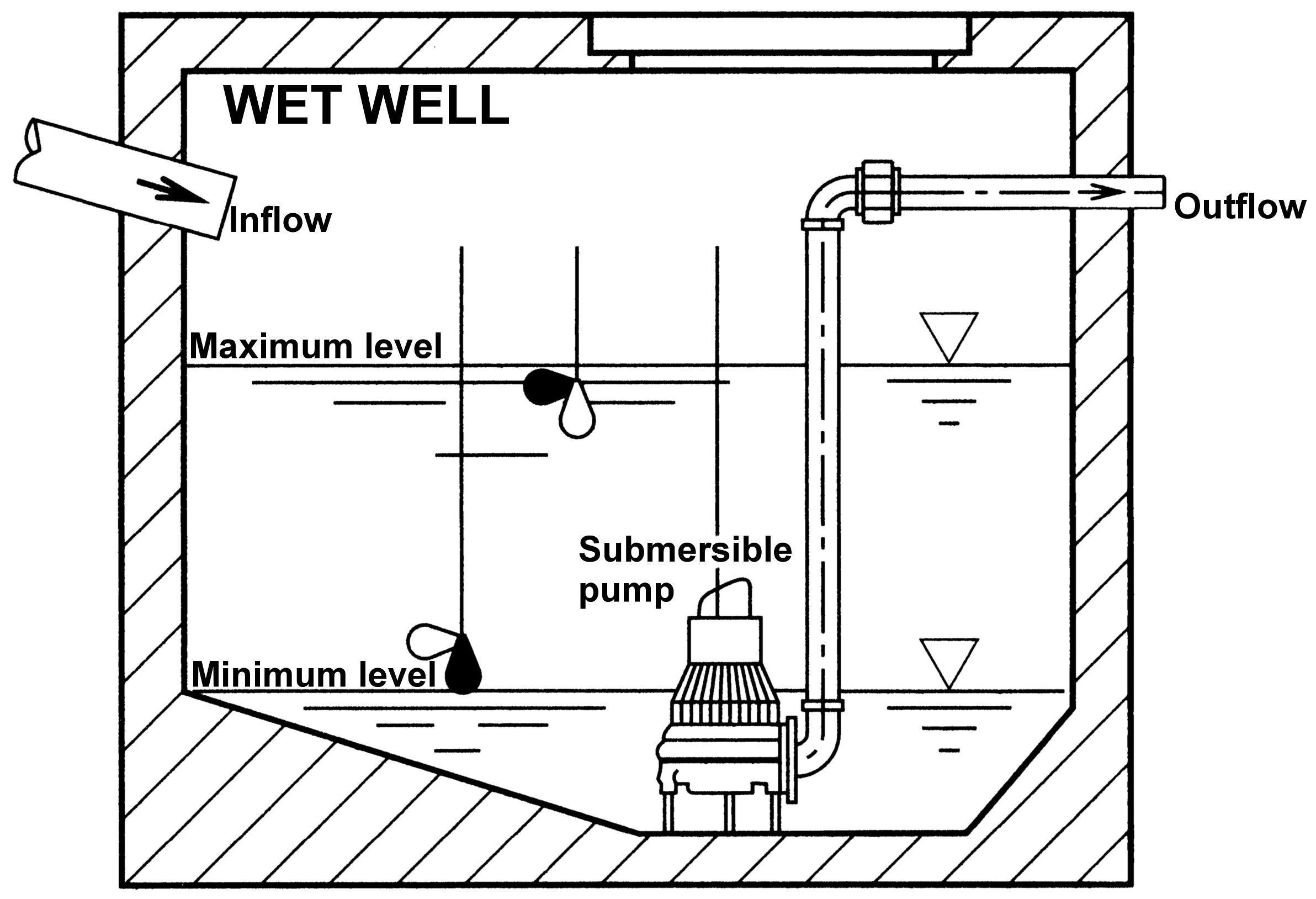
2. Pumping Station Description and Case Study

2.1. Classical Design

A pumping station is designed to collect and transport water to a point of higher elevation. The inflow water is stored in a wet well, where the submersible pump is located. In larger plants, surface pumps could be alternatively installed into dry wells and connected to the tank with a suction pipe. The pump lifts the water through a pressurized pipe toward another collecting system (i.e., a tank or a channel). Generally, the pumps work at constant rotational speed and fairly constant discharge, while the inflow is time dependent. If the grid frequency is not modified (i.e., 50 Hz in EU and 60 Hz in USA) the motor velocity (N) attains its maximum value $N_{max}$. The difference between the inflow and the outflow causes modifications to the water level within the wet well. The classical control of the constant speed (CS) pump is based on the water level: when it rises above a certain level the pump is started. The pump is selected so that its discharge is higher than the maximum inflow: in this way, as the pump is started, the water level decreases. As the water level reaches a minimum value, the pump is turned off and the cycle starts again. A sketch of the wet well is shown in Figure 1.

In the larger pumping stations, two or more pumps are placed to work in parallel, and different water levels are set to start and stop each of the parallel pumps. Since each pump operates in constant conditions, it is selected so that, at the selected discharge (Q), it exhibits the maximum efficiency. In other words, the designed outflow corresponds to the Best Efficiency Point (BEP) of the pump ($Q_{N_{max}}^{BEP}$). The time interval between two consecutive starts of the pump, $\tau$, with $Q^{in}$ inflow discharge, is then equal to:

$$\tau =W\frac{Q_{N_{max}}^{BEP}}{Q^{in}(Q_{N_{max}}^{BEP}-Q^{in})}$$

(1)

where W is the volume of water stored between the maximum and the minimum water levels within the well. The number of starts per hour, $S^h$ can be calculated as:

$$S^h=\frac{3600}{\tau }$$

(2)

where $\tau$ is expressed in seconds. If the inflow discharge $Q_{in}$ is considered as a $\theta$ portion of the $Q_{N_{max}}^{BEP}$, then the number of starts per hour can be written as:

$$S^h=3600\frac{Q_{N_{max}}^{BEP}}{W}\theta (1-\theta )$$

(3)

where the volume W is expressed in m${}^3$, $Q_{N_{max}}^{BEP}$ in m${}^3$/s and $S^h$ in starts per hour. For a wet well with a single pump, in order to avoid that the number of starts per hour ($S^h$) exceeds the maximum value indicated by the pump manufacturer ($S_{max}^h$), the value of $\theta$ must be set to $0.5$, as it can be demonstrated by deriving Equation (3) with respect to $\theta$. Then, the volume can be calculated as:

$$W=900\frac{Q_{N_{max}}^{BEP}}{S_{max}^h}$$

(4)

This formula, that relates the volume of the wet well only to the characteristics of the chosen pump, ensures that the number of starts per hour will never exceed the maximum allowed value, whatever the inflow discharge. The maximum number of starts occurs when the inflow discharge is the half of $Q_{N_{max}}^{BEP}$ and reduces otherwise. The choice of the pump in the design is crucial: a larger pump allows dealing with larger inflow discharge, but implies an increase of the volume, with a subsequent increase of the building costs and of the retention time. The latter can be calculated as the ratio between the volume of the well and the average input discharge [36]. The retention time should be kept short to avoid septicity in the tank if it collects sewage or wastewater. The effect of the pump choice is discussed hereafter.

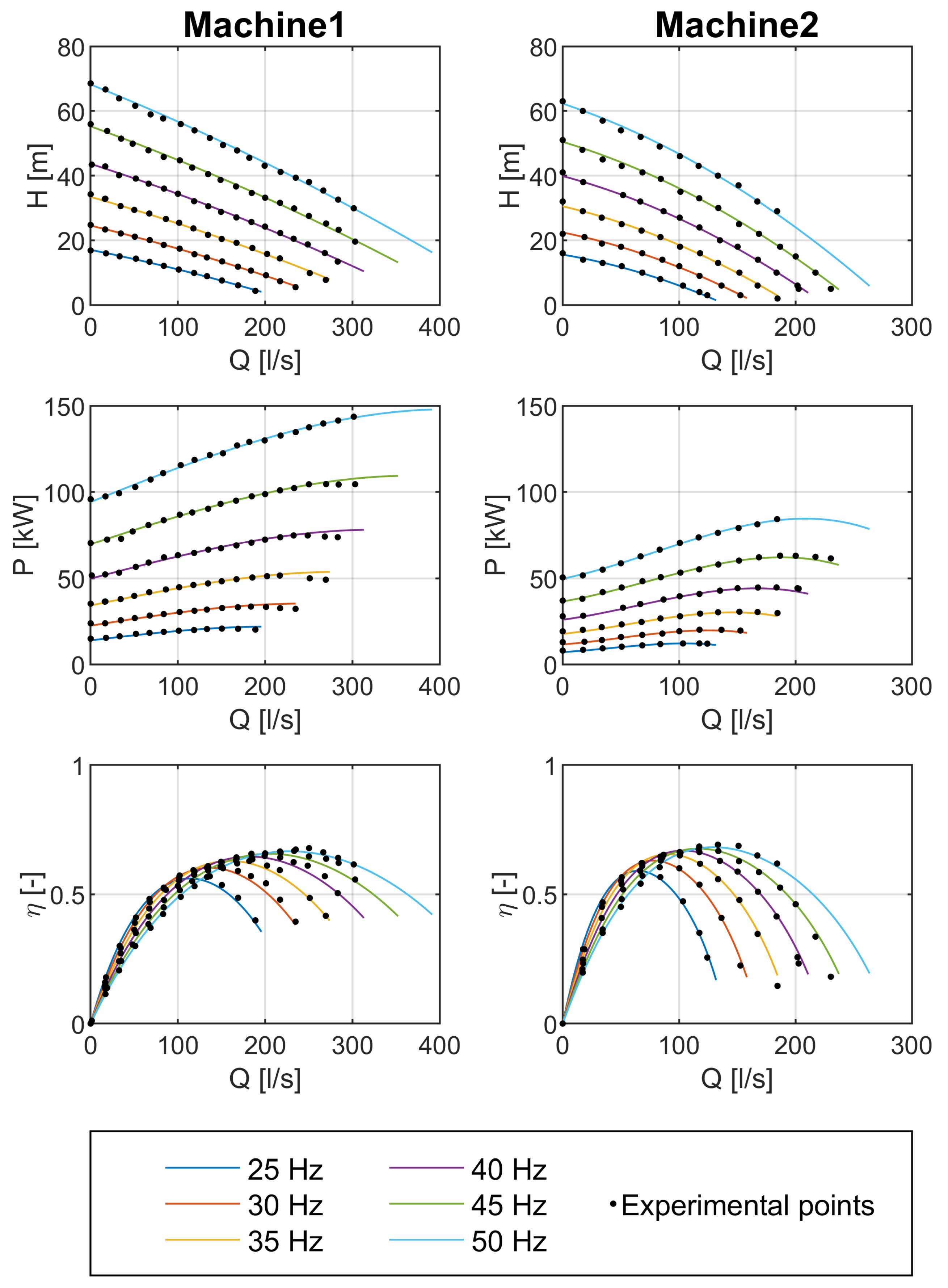
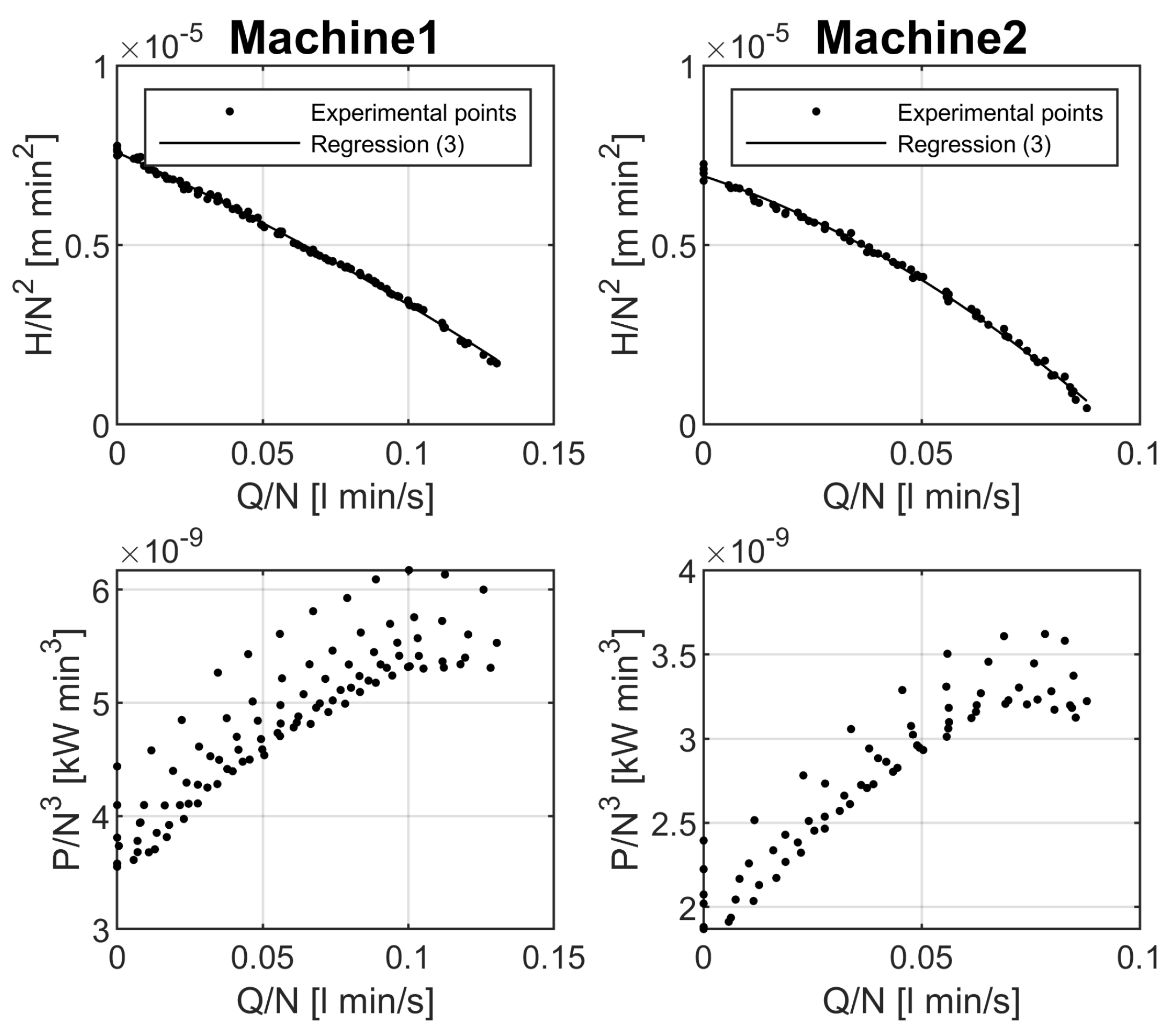
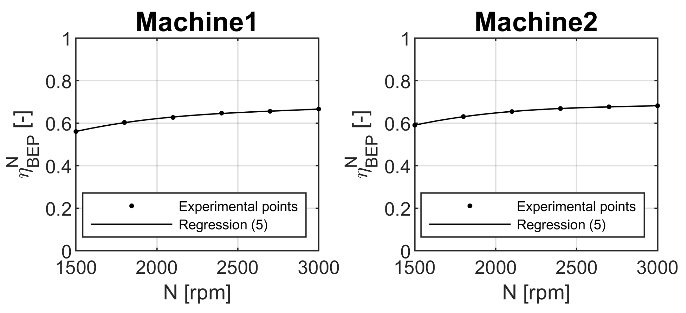
2.2. Experimental Investigation of the Behaviour of Two Submersible Pumps

Two submersible sewage pumps have been tested in the HELAB, the HydroEnergy Laboratory of the University of Naples (CeSMA). The laboratory has been specifically designed for the experimental tests of turbomachines according to ISO 9906 regulation. A large underground storage reservoir (110 m${}^3$ of water) is used to feed the pump. The pumps were located on the bottom of the tank and connected to a 250 mm pipe that conveyed the water through an electro-magnetic discharge meter (accuracy < 0.5%) and then back to the tank. The pressure was measured with a piezoelectric transducer (accuracy < 0.5%). A digital power meter (accuracy < 0.5%) was used to measure the input power. A SCADA system ensured the automatic and simultaneous acquisition of the data. A speed-driver was used to modify the electric frequency (f) and to regulate the speed of the asynchronous motor. For each of the six tested frequencies (50, 45, 40, 35, 30 and 25 Hz respectively), a gate valve was used to set different discharge values. For each discharge, all the measurements were averaged on 500 samples (with a $0.01$ s sampling rate) to reduce the fluctuation of the signal. For each of the two pumps, the maximum number of starts per hour, namely $S_{max}^h$ suggested by the manufacturer is 10. Thus, a complete set of experimental points of discharge (Q), head (H), power (P) has been obtained. The rotational speed (N, in rpm) of the pump can be calculated (if the slip of the motor is neglected) by:

$$N=\frac{60f}{p_p}$$

(5)

where $p_p$ is the number of pole pairs of the motor. The efficiency ($\eta$) has been calculated as the ratio between the hydraulic and the electric power:

$$\eta =\frac{\gamma HQ}{P}$$

(6)

being $\gamma$ the specific weight of water, equal to 9806 N/m${}^3$. For each frequency, the head curve ($H_N(Q)$) and the power curve ($P_N(Q)$) can be interpolated by a polynomial regression (second and third order respectively). Thus, the efficiency can be calculated by Equation (6).

Figure 2 displays the experimental points and the interpolation curves of the two pumps. The best efficiency of both pumps decreases as the frequency decreases. Turbomachinery affinity laws can be used to simulate the pump behaviour under variable speed [37,38] but, unfortunately, they do not get the efficiency reduction [39,40,41]. Indeed, Figure 3 shows that the dispersion of experimental point on the chart ($Q/N,H/N^2$) is negligible, while it is considerable in the chart ($Q/N,P/N^3$).

Thus, according to affinity laws, a unique interpolating polynomial curve (calculated on all the experimental points) has been used to calculate the head, namely:

$$H_N=\left[c_h^2{\left(\frac{Q}{N}\right)}^2+c_h^1\left(\frac{Q}{N}\right)+c_h^0\right]·N^2$$

(7)

while, for the power, a polynomial best fit has been calculated only for $f=50$ Hz, i.e., $N=N_{max}=3000$ rpm on the values of $p^{N_{max}}$

$$p_{N_{max}}=c_p^3{\left(\frac{Q}{N_{max}}\right)}^3+c_p^2{\left(\frac{Q}{N_{max}}\right)}^2+c_p^1\left(\frac{Q}{N_{max}}\right)+c_p^0$$

(8)

being ${\displaystyle p_{N_{max}}=\frac{P_{N_{max}}}{{N_{max}}^3}}$. In order to calculate the power for any N rotational speed, a correction to the affinity laws should be introduced. For each N rotational speed, the best efficiency (${\eta }_{BEP}^N$) can be calculated as:

$${\eta }_N^{BEP}=c_{\eta }^2{N}^2+c_{\eta }^{1}N+c_{\eta }^0$$

(9)

where N is the speed of the pump calculated by Equation (5), as shown by Figure 4.

Thus, a new parameter can be introduced, namely the relative efficiency e [42]:

$$e=\frac{{\eta }_N(Q)}{{\eta }_N^{BEP}}$$

(10)

As shown by Figure 5, the data $(Q/N,e)$ lies on the same curve, with a little dispersion. Thus, for each value of Q and N, e can be calculated by a polynomial regression on $(Q/N)$

$$e=c_e^3{\left(\frac{Q}{N}\right)}^3+c_e^2{\left(\frac{Q}{N}\right)}^2+c_e^1\left(\frac{Q}{N}\right)+c_e^0$$

(11)

while the efficiency can be calculated by Equation (10). Finally, the power P can be calculated by coupling Equations (6) and (8)–(10):

$$P_N(Q)=p_{N_{max}}·N^3·e·{\eta }_N^{BEP}$$

(12)

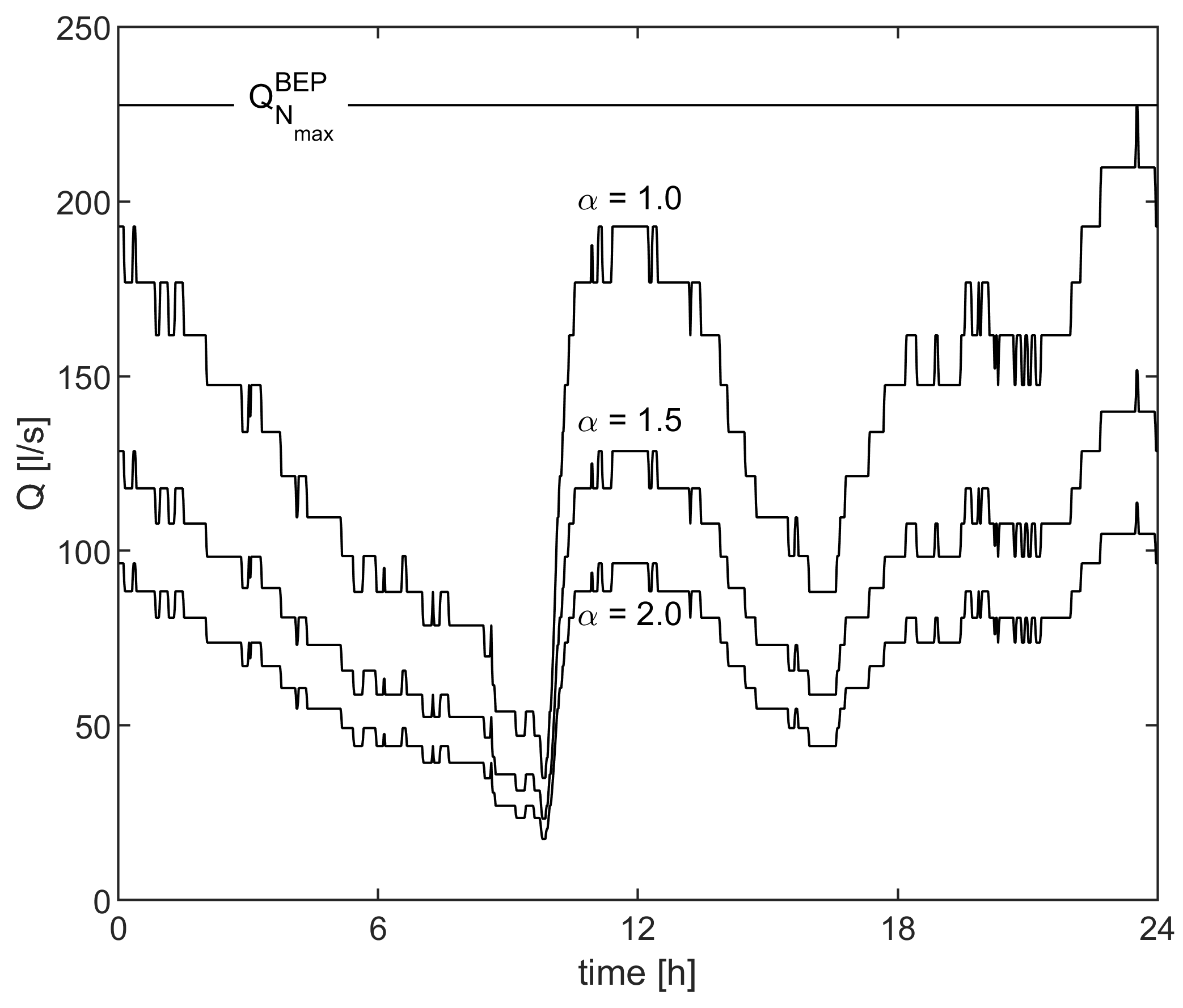
2.3. Input Discharge Pattern

Data used in the present study describe the wastewater flow arriving at the pumping station of Coroglio (Naples, Italy) and collected along the “Arena S. Antonio” (ASA) urban basin. ASA is the largest drainage basin in Western Naples (Italy), having a total area of 1760 ha and a length of the main channel equal to 8.5 km. Originally, it was a stormwater sewer system, but after a strong urbanization of the area it now collects wastewater as well [43]; the catchment is mainly urbanized, with a total percentage of impervious area equal to 62%. The sewer starts at 159 m a.s.l., whereas its terminal section, located at Coroglio treatment plant, has an average altitude of 1 m a.s.l. Different cross-section configurations occur along the main sewer, with a terminal rectangular cross-section with a width of 9 m and a height of 3.7 m.

Runoff data is expressed in terms of water depth in the channel cross-section; data were recorded by means of an ultrasound level gauge at the terminal section of the sewer, 80 m before the pre-treatment plant in Coroglio. The time step of the recording is 90 s. The modelling of the whole system, described in [44], allowed for the estimation of the head-discharge relation for the measurement section and the subsequent estimation of flow rates corresponding to measured heads in dry periods of the year 2016. In the present paper, flow rates describing the daily wastewater pattern of the ASA basin for the day with maximum average daily discharge, which occurred on 18 June 2012 and were aggregated at the time scale of 15 min, were adopted.

The scaled daily pattern $q(t)$ was obtained dividing the measured discharge $Q_{exp}(t)$ by its maximum value:

$$q(t)=\frac{Q_{exp}(t)}{max(Q_{exp})}$$

(13)

Then, for each simulation, the input discharge was calculated setting the maximum input flow rate $Q_{max}^{in}$ as a fraction of the BEP discharge $Q_{BEP}^{N_{max}}$:

$$Q_{max}^{in}=\frac{Q_{N_{max}}^{BEP}}{\alpha }$$

(14)

where $\alpha$ is a coefficient that in this study has been set to 1, $1.5$ and 2. The value of $\alpha$ affects two aspects of the design of the pumping station. For an assigned inflow pattern, higher values of $\alpha$ lead to an oversized plant, with a larger pump, and then a larger wet well (see (4)). On the contrary, the resilience of the plant is higher, because, even if the maximum inflow discharge increases more than the design value, the pump is able to deal with it. Once the value of $\alpha$ was set, then the input discharge pattern $Q_{in}(t)$ was obtained:

$$Q_{in}(t)=q(t)·Q_{max}^{in}$$

(15)

The input pattern, and the effect of $\alpha$ on it, is shown in Figure 6 with reference to the BEP discharge of the first machine.

2.4. Plant Behaviour

The pumping head $H_{man}$ can be calculated from the pumping discharge, by using a quadratic head-loss formula,

$$H_{man}=H_0-H_w(t)+K{Q_p(t)}^2$$

(16)

$H_0$ being the static head when the wet well is empty, $H_w$ the water level in the wet well, depending on time t and K a coefficient depending on the material and the diameter of the outlet pipe. $H_0$ can be set as a ratio of the BEP head at maximum speed $H_{N_{max}}^{BEP}$, namely $\beta$:

$$\beta =\frac{H_0}{H_{N_{max}}^{BEP}}$$

(17)

If the pump is correctly designed, the pumping head $H_{man}$ corresponding to $Q_{N_{max}}^{BEP}$ is close to $H_{N_{max}}^{BEP}$. Then, the coefficient K can be calculated as follows:

$$K=\frac{H_{N_{max}}^{BEP}-H_0}{{Q_{N_{max}}^{BEP}}^2}=\frac{H_{N_{max}}^{BEP}-\beta H_{N_{max}}^{BEP}}{{Q_{N_{max}}^{BEP}}^2}$$

(18)

The effect of $\beta$ on the plant head curve is showed in Figure 7, together with the pump head curves.

The water level into the wet well $H_w$ can be calculated by the continuity equation:

$$Q_{in}(t)-Q_p(t)=\frac{d{W}_w}{dt}$$

(19)

$W_w$ being the volume of water inside the wet well. If S is the cross section of the wet well, then $W_w=S·H_w$. Thus, from the continuity equation, the water level in the wet well can be written as:

$$H_w(t)=H_w(t-dt)+\frac{Q_{in}(t)-Q_p(t)}{S}dt$$

(20)

3. Optimization Model

The optimization model has been written in order to minimize the energy requested to pump the water out of the wet well. Thus, the objective function $E_T$ has been set as follows:

$$E_T={\int }_{T}P(t)dt$$

(21)

T being the time window and $P(t)$ the instantaneous power requested by the pump at the instant t. This equation should be of course discretized, in order to be solved. Thus, the optimizing function becomes:

$$E_T=\sum _{i=1}^{n_T}{P}_i\Delta t$$

(22)

i being the generic time interval whose length is $\Delta t$. During $\Delta t$, each variable is assumed constant. For each i time interval, the power $P_i$ is a function of the rotational speed of the pump ($N_i$) and of the pumped discharge ($Q_i$), as expressed by Equation (12). Furthermore, the pump can be either switched on or off. Thus, a new binary variable has been added, namely the switch $I_i$, which is equal to 1 if the pump is on at the i-th interval, and 0 otherwise. Thus, the requested power for each time interval can be calculated as follows:

$$P_i=P(Q_i,N_i,I_i)=\left({p^{N_{max}}}_i·N_i^3·e_i·{\eta }_{BEP}^N\right)·I_i$$

(23)

From Equation (23), the power at each time interval appears as a function of the discharge, the rotational speed and the switch. The rotational speed can be set between the value corresponding to the maximum grid frequency (namely 50 Hz, corresponding to 3000 rpm) and cannot be lower than 1500 rpm to avoid a danger heating of the machine [45]. Once the rotational speed is selected, the discharge can be calculated: if the pump is switched off, the discharge is obviously zero; otherwise, it can be calculated by equating the head curve of the pump in Equation (7) and that of the plant in Equation (16), as follows:

$$H_0-{H_w}_i+K{Q_i}^2=c_h^2{Q_i}^2+c_h^1{Q}_i{N}_i+c_h^0{N_i}^2$$

(24)

The water level in the wet well, ${H_w}_i$ that appears in Equation (24) is related to the continuity equation, namely Equation (20), which can be written by applying a centered finite difference scheme:

$${H_w}_i={H_w}_{i-1}+\frac{{Q_{in}}_i+{Q_{in}}_{i-1}-Q_i-Q_{i-1}}{2S}\Delta t$$

(25)

Actually, only the speed and the switch are independent variables, while the discharge and the water level in the wet well could be calculated by means of Equations (24) and (25). Nevertheless, in order to improve the coding, they can be set as decision variables, subjected to some constraints. In addition to Equation (25), which is a linear constraint involving ${H_w}_i$ and $Q_i$, the pumped discharge of each time step can be set between a maximum and a minimum value, as follows:

$$0\le Q_i\le Q_{max}^{ad}·I_i$$

(26)

The right side of such a constraint is written to force the discharge to zero if the pump is switched off. $Q_{max}^{ad}$ is set to a high value, e.g., 3 times $Q_{BEP}$. Furthermore, the momentum equation can be modified as follows, in order to include the switch ($I_i$):

$$(H_0-{H_w}_i)·I_i+K{Q_i}^2=c_h^2{Q_i}^2+c_h^1{Q}_i{N}_i+c_h^0{N_i}^2·I_i$$

(27)

Such equality is satisfied if the pumping head equals the plant equation and collapses to an identity if the pump is switched off. Moreover, a minimum and a maximum bond are fixed also for the water level in the wet well:

$$H_w^{min}\le {H_w}_i\le H_w^{max}$$

(28)

Finally, a last constraint that involves $I_i$ can be written, considering the maximum allowable starts per hour of the pump ($S_{max}^h$). This last non-linear constraint can be written with reference to a new variable, that counts the number of starts for each one-hour window, ${S^h}_i$, that is a non linear function of $I_i$. It can be calculated as the sum of the occurrence of the event $(I_j-I_{j-1})>0$), where j is the generic time interval of a one-hour window before the i instant. Hence,

$${S^h}_i\le S_{max}^h$$

(29)

All the equations written above can be summarized in the following model, written for the T time window:

$$\left\{\begin{array}{c}\begin{array}{cc}\hfill \underset{N_i,I_i,Q_i,{H_w}_i}{minimize}& E_T=\sum _T{P}_i\Delta t\hfill \\ \hfill \mathrm{subject}\mathrm{to}& \begin{array}{c}(H_0-{H_w}_i)·I_i+K{Q_i}^2=c_h^2{Q_i}^2+c_h^1{Q}_i{N}_i+c_h^0{N_i}^2·I_i\hfill \\ {H_w}_i={H_w}_{i-1}+\frac{{Q_{in}}_i+{Q_{in}}_{i-1}-Q_i-Q_{i-1}}{2S}\Delta t\hfill \\ 0\le Q_i\le Q_{max}^{ad}·I_i\hfill \\ 1500\le N_i\le 3000\hfill \\ 0\le I_i\le 1\hfill \\ H_w^{min}\le {H_w}_i\le H_w^{max}\hfill \\ {S_h}_i\le S_{max}\hfill \\ I_i\in \mathbb{Z},Q_i\in \mathbb{R},N_i\in \mathbb{R}\hfill \\ \forall i=1\dots n_T\hfill \end{array}\hfill \end{array}\hfill \end{array}\right.$$

(30)

Resolution of the Optimization Model

The optimization problem involves linear and non linear constraints, continuous and integer variables and the objective is a non linear function of the selected variables. The problem is classified as mixed integer non linear problem (MINLP). The Basic Open-source Nonlinear Mixed INteger programming (BONMIN) [46] code has been chosen to solve the optimization. The selected algorithm is a branch-and-bound based algorithm [47] specifically designed for mixed integer non linear problems and has been successfully used in hydraulic problems in recent times [48]. For each step, the algorithm solves the continuous relaxed problem through the Interior Point OPTimizer (IPOPT) [49] and the Coin-or branch and cut (Cbc) algorithm [50] to solve the mixed integer problem. Even if the algorithm is designed for convex problems, it can retrieve heuristic solutions in case of non-convex problems [51]. The problem described by Equation (30) is quite complex and the convexity has not been proven herein. Thus, all the options for the resolution of non-convex problems have been selected.

The problem can be quite large, depending on the choice of the time window, T, and the length of the time interval, $\Delta t$. Each of the four variables is a vector with $n_T$ elements, while the 11 constraints in Equation (30) can be written for any i interval. Thus the problem has $4·n_T$ variables and $11·n_T$ constraints. A Mixed Integer Non Linear Programming is classified as a NP-hard problem [52], where the computational time and resources exponentially increase with the number of variables. If the input pattern is considered periodic, i.e., the pattern keeps happening every day, the optimization should be performed on the whole daily pattern. The choice of the length of the time interval $\Delta t$ is crucial: it cannot be too short, in order to avoid a too large number of variables, while a too long interval produces unreliable results, due to the coarse discretization of the problem. Furthermore, the filling time (with the maximum input discharge) of a wet well is generally lower than thousands of seconds: then, $\Delta t$ should be lower than the filling time, in order to avoid the complete filling of the wet well when the pump is switched off. In this paper, $\Delta t$ has been chosen equal to 60 s.

Thus, in order to get reliable results in a reasonable time, once $\Delta t$ has been chosen, the whole day has been divided in $n_w$ time windows of T length (being $n_w·T=1day$), and the optimization problem has been solved for each of them. The optimal solution for the whole day, i.e., the optimal sequence of speeds and switches, has been obtained as the union of $n_w$ consecutive solutions. Hence, the optimal daily energy, $E_{opt}$, can be calculated as the sum of the energy of each time window $E_T$:

$$E_{opt}=\sum _{T=1}^{n_w}{E}_T$$

(31)

In this way, only a nearly-optimal solution can be found, and in this paper the dependency of the results on the length of the window has been investigated.

4. Application and Results

The optimization model has been applied to several different situations. Two different wet wells have been designed for the two pumps, based on Equation (4), resulting in $W=26.6$ m${}^3$ and $15.19$ m${}^3$ respectively. A constant cross section wet well has been chosen, with a 10 m${}^2$ base surface, then $H_{max}$ results 2.66 m and 1.52 m respectively. Different scenarios have been created by selecting the values of the $\alpha$ and the $\beta$ coefficients. This means that, assigned the pump (machine 1 or 2), different input patterns have been calculated by setting the $\alpha$ value equal to 1, $1.5$ and 2 respectively. The resulting values of $Q_{max}^{in}$ are shown in

Table 1. Parameters of 30 the different studied scenarios, resulting from the choice of the machine and different values of $\alpha$ and $\beta$.

Machine	$\mathit{\alpha }$	$\mathit{\beta }$	${\mathit{Q}}_{\mathit{max}}$	${\mathit{H}}_0$	${\mathit{E}}_{\mathit{ref}}$	${\mathit{E}}_{\mathit{cs}}$
[-]	[-]	[-]	[L/s]	[m]	kWh/day	kWh/day
1	1.00	0.00	236.66	0.00	616.9	1960.8
1	1.00	0.25	236.66	9.71	790.4	1956.7
1	1.00	0.50	236.66	19.42	963.9	1951.0
1	1.00	0.75	236.66	29.13	1137.4	1939.4
1	1.00	1.00	236.66	38.84	1310.8	1914.4
1	1.50	0.00	157.78	0.00	182.8	1305.5
1	1.50	0.25	157.78	9.71	355.6	1306.0
1	1.50	0.50	157.78	19.42	528.3	1298.8
1	1.50	0.75	157.78	29.13	701.1	1291.5
1	1.50	1.00	157.78	38.84	873.9	1274.7
1	2.00	0.00	118.33	0.00	77.1	978.1
1	2.00	0.25	118.33	9.71	221.7	979.5
1	2.00	0.50	118.33	19.42	366.3	975.6
1	2.00	0.75	118.33	29.13	510.8	969.0
1	2.00	1.00	118.33	38.84	655.4	957.2
2	1.00	0.00	135.04	0.00	356.5	1112.8
2	1.00	0.25	135.04	9.83	456.7	1113.7
2	1.00	0.50	135.04	19.67	557.0	1110.7
2	1.00	0.75	135.04	29.50	657.2	1106.2
2	1.00	1.00	135.04	39.33	757.5	1098.3
2	1.50	0.00	90.03	0.00	105.6	743.7
2	1.50	0.25	90.03	9.83	205.5	741.7
2	1.50	0.50	90.03	19.67	305.3	739.3
2	1.50	0.75	90.03	29.50	405.2	738.7
2	1.50	1.00	90.03	39.33	505.0	732.2
2	2.00	0.00	67.52	0.00	44.6	557.0
2	2.00	0.25	67.52	9.83	128.1	556.3
2	2.00	0.50	67.52	19.67	211.7	554.5
2	2.00	0.75	67.52	29.50	295.2	554.7
2	2.00	1.00	67.52	39.33	378.7	549.5

. Different plants have been simulated by setting $\beta$ equal to 0, $0.25$, $0.5$, $0.75$ and 1 respectively, resulting in different values of $H_0$ and head loss. For each scenario, a reference value of daily requested energy, namely $E_{ref}$ has been calculated, as follows:

$$E_{ref}={\int }_{day}\gamma Q^{in}(t)[H_0+K{Q^{in}}^2(t)]dt$$

(32)

Each scenario has been optimized, setting a time window of 30 min and a $\Delta t$ of 1 min, so that $n_T=30$. Thus, for each time window, 120 optimal variables have been found. For the first instant of the day, the water level within has been set as half of the maximum level.

Table 2. Results of the optimization with a time window of 30 min (C.T.—computational time).

Machine	$\mathit{\alpha }$	$\mathit{\beta }$	${\mathit{E}}_{\mathit{ref}}$	${\mathit{E}}_{\mathit{cs}}$	${\mathit{E}}_{\mathit{opt}}$	${\mathit{\eta }}_{\mathit{cs}}$	${\mathit{\eta }}_{\mathit{opt}}$	$\mathit{\epsilon }$	C.T.
[-]	[-]	[-]	[kWh/day]	[kWh/day]	[kWh/day]	[-]	[-]	[-]	[min]
1	1.0	0.00	616.9	1960.8	924.5	0.315	0.667	2.121	1.8
1	1.0	0.25	790.4	1956.7	1132.3	0.404	0.698	1.728	1.3
1	1.0	0.50	963.9	1951.0	1404.9	0.494	0.686	1.389	1.6
1	1.0	0.75	1137.4	1939.4	1684.4	0.586	0.675	1.151	1.4
1	1.0	1.00	1310.8	1914.4	1924.8	0.685	0.681	0.995	2.4
1	1.5	0.00	182.8	1305.5	384.2	0.140	0.476	3.398	6.6
1	1.5	0.25	355.6	1306.0	541.9	0.272	0.656	2.410	1.6
1	1.5	0.50	528.3	1298.8	829.3	0.407	0.637	1.566	21.2
1	1.5	0.75	701.1	1291.5	1129.8	0.543	0.621	1.143	904.6
1	1.5	1.00	873.9	1274.7	1321.8	0.686	0.661	0.964	3.0
1	2.0	0.00	77.1	978.1	284.5	0.079	0.271	3.438	5.4
1	2.0	0.25	221.7	979.5	373.5	0.226	0.594	2.623	1.4
1	2.0	0.50	366.3	975.6	622.6	0.375	0.588	1.567	2906.8
1	2.0	0.75	510.8	969.0	867.2	0.527	0.589	1.117	383.3
1	2.0	1.00	655.4	957.2	1004.3	0.685	0.653	0.953	3.5
2	1.0	0.00	356.5	1112.8	538.5	0.320	0.662	2.067	2.3
2	1.0	0.25	456.7	1113.7	660.5	0.410	0.692	1.686	1.2
2	1.0	0.50	557.0	1110.7	817.6	0.501	0.681	1.358	28.6
2	1.0	0.75	657.2	1106.2	975.0	0.594	0.674	1.135	1.4
2	1.0	1.00	757.5	1098.3	1093.7	0.690	0.693	1.004	2.5
2	1.5	0.00	105.6	743.7	218.8	0.142	0.483	3.399	2.2
2	1.5	0.25	205.5	741.7	316.9	0.277	0.648	2.340	1.6
2	1.5	0.50	305.3	739.3	484.7	0.413	0.630	1.525	16,559.1
2	1.5	0.75	405.2	738.7	643.4	0.548	0.630	1.148	1.6
2	1.5	1.00	505.0	732.2	740.0	0.690	0.682	0.990	2.6
2	2.0	0.00	44.6	557.0	159.3	0.080	0.280	3.496	2.5
2	2.0	0.25	128.1	556.3	214.4	0.230	0.598	2.595	1.3
2	2.0	0.50	211.7	554.5	362.8	0.382	0.583	1.529	977.0
2	2.0	0.75	295.2	554.7	486.9	0.532	0.606	1.139	2.1
2	2.0	1.00	378.7	549.5	562.0	0.689	0.674	0.978	2.5

shows the values of energy required by the optimal solution $E_{opt}$, as well as the calculated values $E_{cs}$, namely the daily energy required by CS pumping station, i.e., a pumping station where the pump operates only at its maximum speed and its starts and stops are controlled only by the water level has been also calculated. Two new parameters, namely ${\eta }_{cs}$ and ${\eta }_{opt}$, calculated as the ratio between $E_{cs}$ or $E_{opt}$ respectively and $E_{ref}$ are also shown.

The values of ${\eta }_{CS}$ demonstrate that, as the maximum inflow approaches the BEP discharge, the efficiency of the pump station increases. Furthermore, the values of ${\eta }_{OPT}$ are even larger than ${\eta }_{CS}$, demonstrating that the optimal regulation allows a better energy efficiency of the system.

The benefit column, namely $\epsilon$, shows the ratio between $E_{cs}$ and $E_{opt}$. The higher $\epsilon$ values are larger than 2 and occur when $\beta$ is zero. This means that, with such an optimization, more than half of the energy requested by the classical operation can be saved. The $\epsilon$ value decreases as $\beta$ increases. Values of $\epsilon$ lower than 1 (resulting from values of $E_{opt}$ slightly higher than $E_{cs}$) occur when $\beta$ is equal to 1. This can be considered a weakness of the model, since the constant speed operation is a feasible solution for the optimization model and should be selected by the algorithm (thus, a $\epsilon$ equal to 1 should be a lower bound). Values of $\epsilon$ slightly lower than 1 could be due either to the discretization or to the non convexity of the problem. Among the different scenarios, an average value of $32\%$ energy can be saved with an optimized control. The last column of the Table shows the computational time. It is highly variable and, even if in the majority of the cases is reasonable, reaches a maximum value of 11.5 days. A pattern of the computational time is apparently not detectable. The unstable behaviour of the optimization algorithm is probably due to the non-convexity of the problem, together with the choice of dividing the entire day in multiple time windows.

Figure 8 shows the dependency of ${\eta }_{cl}$ and ${\eta }_{opt}$ on $\alpha$ and $\beta$. The efficiency of the optimal regulation is generally larger than the efficiency of the classical regulation, but, the difference reduces as $\beta$ increases, i.e., the head loss reduces. The efficiency of both systems is higher when $\alpha$ is lower and when $\alpha$ is equal to 1 the efficiency of the optimal regulation is close to the maximum value, independently from the value of $\beta$. The efficiency of the optimal scheduling is fairly constant as $\beta$ exceeds $0.25$. This means that, if the head loss changes during the life of the plant, the efficiency of the system can be kept constant during the years through an optimal scheduling of the pump operations.

Figure 9 shows the benefit, $\epsilon$, that can be obtained when the optimal regulation is used to replace the classical system. Such a benefit decreases as $\beta$ increases, i.e., as the head loss reduces, following the behaviour of ${\eta }_{CS}$ and ${\eta }_{OPT}$. The reduction of the benefit as $\beta$ increases is due to two reasons: when the head loss reduces, a reduction in the output discharge produces smaller reductions in the required head, as shown in Figure 7. Consequently, the total energy required to pump the entire volume of water slightly depends on the output discharge. Furthermore, as shown in Figure 7, as $\beta$ approaches 1, the plant line intersects regions of the pump performance where the efficiency is lower. Thus, a speed regulation aimed at a reduction of the outflow discharge becomes less effective.

The highest value of $\epsilon$ is $3.44$ and occurs when $\alpha$ is equal to $2.0$ and $\beta$ is equal to zero. This means that up to more than $70\%$ energy can be saved. A similiar behaviour occurs for $\alpha$ equal to $1.5$. Lower benefits can be obtained when $\alpha$ is equal to 1.

For the first five scenarios, the dependency of the best solution on the time window has been tested, repeating the optimization with a time window of 60 and 120 min respectively. In each of the three cases, the timestep is fixed and equal to 1 min. The results are shown in

Table 3. Comparison of the optimization results with different values of time window (T).

T	${\mathit{E}}_{\mathit{opt}}$	${\mathit{\eta }}_{\mathit{opt}}$	$\mathit{\epsilon }$	C.T.
[min]	[kWh/day]	[-]	[-]	[min]
30	924.5	0.667	2.121	1.8
30	1132.3	0.698	1.728	1.3
30	1404.9	0.686	1.389	1.6
30	1684.4	0.675	1.151	1.4
30	1924.8	0.681	0.995	2.4
60	920.8	0.670	2.129	1.8
60	1127.9	0.701	1.735	1.5
60	1399.3	0.689	1.394	2.0
60	1676.7	0.678	1.157	1.8
60	1910.2	0.686	1.002	2.2
120	918.6	0.672	2.135	6.6
120	1125.7	0.702	1.738	2.4
120	1396.5	0.690	1.397	3.4
120	1672.6	0.680	1.159	2.0
120	1902.0	0.689	1.007	3.5

. The improvement in terms of saved energy is really low, demonstrating that a time window of 30 min is sufficient to get the optimal result.

5. Conclusions

In the present paper, an optimization problem is described concerning the pump scheduling of a drainage pumping station. Compared to current literature, the main difficulty lies in the pump rotational speed, that is able to vary in a given range altering the usual operational field of the machine. To comply with the peculiarities of the problem, the paper is structured into several consecutive steps:

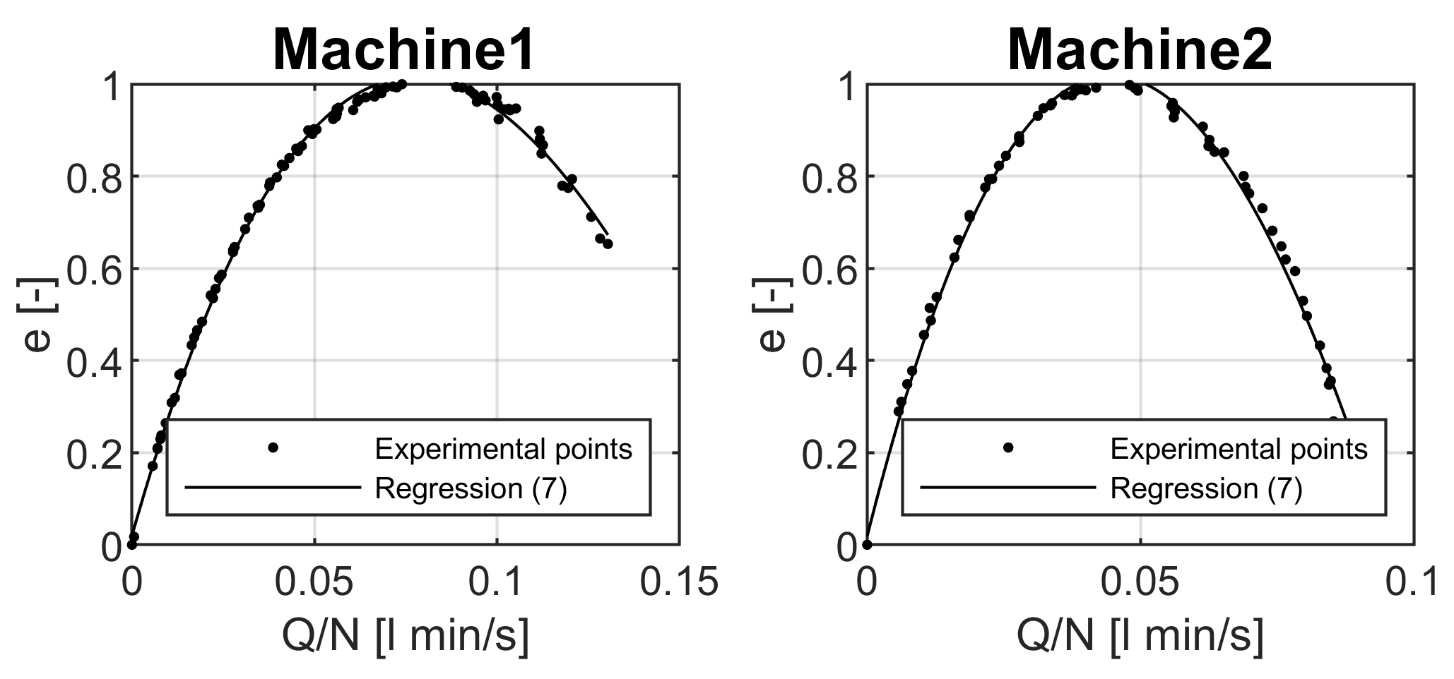
• An experimental campaign is undertaken to explore the effects of variable speed on the pumping efficiency. Specifically, in accordance with the affinity laws, an empirical equation is provided to compute the pumping head (Equation (7)), whereas a novel approach based on the concept of relative efficiency (Equation (10)) is provided to compute the pumping power under variable speed conditions (Equation (12)).
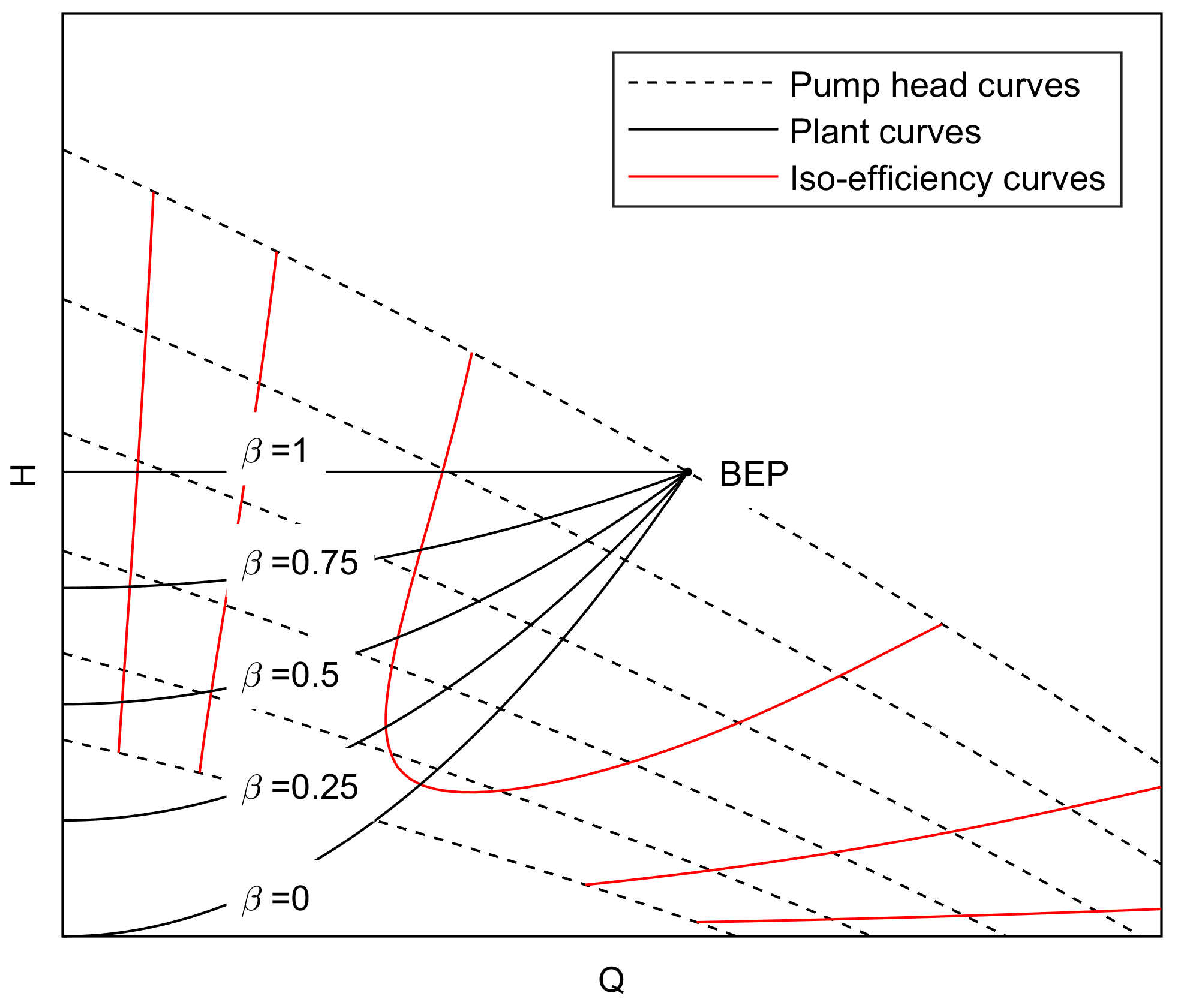
• On the basis of the above-mentioned theoretical framework, a mixed-integer optimization problem (Equation (30)) is built that is made up of an objective function (the overall pumping energy) to be minimized and a set of constraints for the variables of interest. The model is also able to comply with the ON/OFF switch of the pump, and two parameters ($\alpha$ and $\beta$) are introduced to simulate different scenarios for the inflow discharge and the plant configuration. The influence of the time window and step for computations is also discussed.
• The model is solved for a case study (a literature sewage daily pattern provided for the City of Naples, Italy) relying on a literature algorithm, and some indicators are analyzed to test the computational performance of the algorithm and the overall energy savings given by the optimal solution for the different scenarios. The case study was developed assuming a known inflow pattern and a constant energy cost during the day.

The optimization results show that, if the pump scheduling, i.e., the pump starts and rotational speed, is optimized, meaningful energy saving can be pursued. The amount of saving depends on the plant characteristics, in terms of inflow discharge and head loss. Among the different simulated scenarios, the average ratio of saved energy is equal to $32\%$, with a peak value of more than $70\%$ in the most convenient scenario. The efficiency of the optimal system increases as the difference between the pump maximum discharge and the inflow decreases, while the effect of the head losses is mild and the efficiency of the optimal scheduling is fairly constant if the head loss is not too high, i.e., the static head is higher than one fourth of the BEP head of the pump. This could mean that the efficiency of an optimal scheduled plant can be kept fairly constant over the years, even if the plant head loss changes due to the wear of the pipeline.Nevertheless, when the head loss of the pumping pipeline reduces to zero, the benefit due to an optimized control, when compared to a classical control based on the water level, becomes negligible. The optimization algorithm that has been implemented showed good performance in terms of computational time, even if in certain cases it extends to several days, with no detectable patterns. In order to keep the optimization problem small, the entire day is divided into multiple time windows. The final solution is the sum of the optimal scheduling of each time window. A final comparison shows that a time window of 30 min is sufficient to detect the optimal solution and a further extension of it does not give significant improvements in terms of energy saving.

This entire study is developed assuming hypothesis of knowing the inflow pattern and considering a constant cost of the energy. Future developments could include (i) the variability of the energy cost during the day, e.g., saving energy during the day and working more during the night and (ii) a real time optimized control to face the random variability of the inflow pattern.

References

1. Carravetta, A.; Fecarotta, O.; Golia, U.M.; La Rocca, M.; Martino, R.; Padulano, R.; Tucciarelli, T. Optimization of Osmotic Desalination Plants for Water Supply Networks. Water Resour. Manag. 2016, 30, 3965–3978. [Google Scholar] [CrossRef] [Green Version]
2. Carravetta, A.; Fecarotta, O.; Ramos, H. A new low-cost installation scheme of PATs for pico-hydropower to recover energy in residential areas. Renew. Energy 2018. [Google Scholar] [CrossRef]
3. Vairavamoorthy, K.; Lumbers, J. Leakage Reduction in Water Distribution Systems: Optimal Valve Control. J. Hydraul. Eng. 1998, 124, 1146–1154. [Google Scholar] [CrossRef]
4. Castro-Gama, M.; Pan, Q.; Lanfranchi, E.A.; Jonoski, A.; Solomatine, D.P. Pump Scheduling for a Large Water Distribution Network Milan, Italy. Procedia Eng. 2017, 186, 436–443. [Google Scholar] [CrossRef]
5. Goldstein, R.; Smith, W. Water & Sustainability: U.S. Electricity Consumption for Water Supply & Treatment—The Next Half Century. Water Supply 2002, 4, 93. [Google Scholar] [CrossRef]
6. Bunn, S.M.; Reynolds, L. The energy-efficiency benefits of pump-scheduling optimization for potable water supplies. IBM J. Res. Dev. 2009, 53, 5:1–5:13. [Google Scholar] [CrossRef]
7. Zhang, Z.; He, X.; Kusiak, A. Data-driven minimization of pump operating and maintenance cost. Eng. Appl. Artif. Intell. 2015, 40, 37–46. [Google Scholar] [CrossRef]
8. Plappally, A.K.; Lienhard, V.J.H. Energy requirements for water production, treatment, end use, reclamation, and disposal. Renew. Sustain. Energy Rev. 2012, 16, 4818–4848. [Google Scholar] [CrossRef]
9. Zhang, Z.; Kusiak, A.; Zeng, Y.; Wei, X. Modeling and optimization of a wastewater pumping system with data-mining methods. Appl. Energy 2016, 164, 303–311. [Google Scholar] [CrossRef]
10. Boulos, P.F.; Wu, Z.; Orr, C.H.; Moore, M.; Hsiung, P.; Thomas, D. Optimal Pump Operation of Water Distribution Systems Using Genetic Algorithms. Available online: https://pdfs.semanticscholar.org/30bd/0b8898b9c7eede6581df60fe8aaf2964d0f7.pdf?_ga=2.184499744.767898400.1542030914-596395705.1542030914 (accessed on 12 November 2018).
11. Ostojin, S.; Mounce, S.R.S.; Boxall, J.B.J. An artificial intelligence approach for optimizing pumping in sewer systems. J. Hydroinform. 2011, 13, 295–306. [Google Scholar] [CrossRef] [Green Version]
12. Carravetta, A.; Antipodi, L.; Golia, U.; Fecarotta, O. Energy saving in a water supply network by coupling a pump and a Pump As Turbine (PAT) in a turbopump. Water 2017, 9, 62. [Google Scholar] [CrossRef]
13. Carravetta, A.; Conte, M.; Antipodi, L. Energy efficiency index for water supply systems. In Proceedings of the AEIT International Annual Conference (AEIT), Naples, Italy, 14–16 October 2015; pp. 1–4. [Google Scholar]
14. Jowitt, P.W.; Germanopoulos, G. Optimal Pump Scheduling in Water? Supply Networks. J. Water Resour. Plan. Manag. 1992, 118, 406–422. [Google Scholar] [CrossRef]
15. Little, K.W.; McCrodden, B.J. Minimization of raw water pumping costs using MILP. J. Water Resour. Plan. Manag. 1989, 115, 511–522. [Google Scholar] [CrossRef]
16. Ormsbee, L.E.; Walski, T.M.; Chase, D.V.; Sharp, W.W. Methodology for Improving Pump Operation Efficiency. J. Water Resour. Plan. Manag. 1989, 115, 148–164. [Google Scholar] [CrossRef]
17. Tabesh, M. Scheduling and operating costs in water distribution networks. Proc. Inst. Civ. Eng. 2013, 166, 432. [Google Scholar]
18. Lansey, K.; Awumah, K. Optimal Pump Operations Considering Pump Switches. J. Water Resour. Plan. Manag. 1994, 120, 17–35. [Google Scholar] [CrossRef]
19. Van Zyl, J.E.; Savic, D.A.; Walters, G.A. Operational optimization of water distribution systems using a hybrid genetic algorithm. J. Water Resour. Plan. Manag. 2004, 130, 160–170. [Google Scholar] [CrossRef]
20. Hashemi, S.S.; Tabesh, M.; Ataeekia, B. Ant-colony optimization of pumping schedule to minimize the energy cost using variable-speed pumps in water distribution networks. Urban Water J. 2014, 11, 335–347. [Google Scholar] [CrossRef]
21. De Paola, F.; Fontana, N.; Giugni, M.; Marini, G.; Pugliese, F. An application of the Harmony-Search Multi-Objective (HSMO) optimization algorithm for the solution of pump scheduling problem. Procedia Eng. 2016, 162, 494–502. [Google Scholar] [CrossRef]
22. De Paola, F.; Fontana, N.; Giugni, M.; Marini, G.; Pugliese, F. Optimal solving of the pump scheduling problem by using a Harmony Search optimization algorithm. J. Hydroinform. 2017, 19, 879–889. [Google Scholar] [CrossRef]
23. Shamir, U.; Salomons, E. Optimal Real-Time Operation of Urban Water Distribution Systems Using Reduced Models. J. Water Resour. Plan. Manag. 2008, 134, 181–185. [Google Scholar] [CrossRef]
24. Alvisi, S.; Franchini, M.; Marinelli, A. A short-term, pattern-based model for water-demand forecasting. J. Hydroinform. 2007, 9, 39. [Google Scholar] [CrossRef]
25. Jamieson, D.G.; Shamir, U.; Martinez, F.; Franchini, M. Conceptual design of a generic, real-time, near-optimal control system for water-distribution networks. J. Hydroinform. 2007, 9, 3. [Google Scholar] [CrossRef]
26. Martínez, F.; Hernández, V.; Alonso, J.M.; Rao, Z.; Alvisi, S. Optimizing the operation of the Valencia water-distribution network. J. Hydroinform. 2007, 9, 65. [Google Scholar] [CrossRef]
27. Rao, Z.; Alvarruiz, F. Use of an artificial neural network to capture the domain knowledge of a conventional hydraulic simulation model. J. Hydroinform. 2007, 9, 15. [Google Scholar] [CrossRef]
28. Barán, B.; Von Lücken, C.; Sotelo, A. Multi-objective pump scheduling optimisation using evolutionary strategies. Adv. Eng. Softw. 2005, 36, 39–47. [Google Scholar] [CrossRef]
29. Wang, J.Y.; Chang, T.P.; Chen, J.S. An enhanced genetic algorithm for bi-objective pump scheduling in water supply. Expert Syst. Appl. 2009, 36, 10249–10258. [Google Scholar] [CrossRef]
30. Kougias, I.P.; Theodossiou, N.P. Multiobjective Pump Scheduling Optimization Using Harmony Search Algorithm (HSA) and Polyphonic HSA. Water Resour. Manag. 2013, 27, 1249–1261. [Google Scholar] [CrossRef]
31. Zeng, Y.; Zhang, Z.; Kusiak, A.; Tang, F.; Wei, X. Optimizing wastewater pumping system with data-driven models and a greedy electromagnetism-like algorithm. Stoch. Environ. Res. Risk Assess. 2016, 30, 1263–1275. [Google Scholar] [CrossRef]
32. Giacomello, C.; Kapelan, Z.; Nicolini, M. Fast Hybrid Optimization Method for Effective Pump Scheduling. J. Water Resour. Plan. Manag. 2013, 139, 175–183. [Google Scholar] [CrossRef]
33. Sperlich, A.; Pfeiffer, D.; Burgschweiger, J.; Campbell, E.; Beck, M.; Gnirss, R.; Ernst, M. Energy Efficient Operation of Variable Speed Submersible Pumps: Simulation of a Ground Water Well Field. Water 2018, 10, 1255. [Google Scholar] [CrossRef]
34. Behandish, M.; Wu, Z.Y. Concurrent pump scheduling and storage level optimization using meta-models and evolutionary algorithms. Procedia Eng. 2014, 70, 103–112. [Google Scholar] [CrossRef]
35. Chabal, L.; Stanko, S. Sewerage pumping station optimization under real conditions. Geosci. Eng. 2014, 60, 19–28. [Google Scholar] [CrossRef]
36. Boon, A.G. Septicity in sewers: Causes, consequences and containment. Water Sci. Technol. 1995, 31, 237–253. [Google Scholar] [CrossRef]
37. Fecarotta, O.; Ramos, H.M.; Derakhshan, S.; Del Giudice, G.; Carravetta, A. Fine Tuning a PAT Hydropower Plant in a Water Supply Network to Improve System Effectiveness. J. Water Resour. Plan. Manag. 2018, 144, 04018038. [Google Scholar] [CrossRef]
38. Pugliese, F.; De Paola, F.; Fontana, N.; Giugni, M.; Marini, G. Performance of vertical-axis pumps as turbines. J. Hydraul. Res. 2018, 1–12. [Google Scholar] [CrossRef]
39. Fecarotta, O.; Carravetta, A.; Ramos, H.M.; Martino, R. An improved affinity model to enhance variable operating strategy for pumps used as turbines. J. Hydraul. Res. 2016, 54, 332–341. [Google Scholar] [CrossRef]
40. Simpson, A.R.; Marchi, A. Evaluating the approximation of the affinity laws and improving the efficiency estimate for variable speed pumps. J. Hydraul. Eng. 2013, 139, 1314–1317. [Google Scholar] [CrossRef]
41. Carravetta, A.; Conte, M.C.; Fecarotta, O.; Ramos, H.M. Evaluation of PAT performances by modified affinity law. Procedia Eng. 2014, 89, 581–587. [Google Scholar] [CrossRef]
42. Morani, M.; Carravetta, A.; Del Giudice, G.; McNabola, A.; Fecarotta, O. A Comparison of Energy Recovery by PATs against Direct Variable Speed Pumping in Water Distribution Networks. Fluids 2018, 3, 41. [Google Scholar] [CrossRef]
43. Padulano, R.; Del Giudice, G. A Mixed Strategy Based on Self-Organizing Map for Water Demand Pattern Profiling of Large-Size Smart Water Grid Data. Water Resour. Manag. 2018, 32, 3671–3685. [Google Scholar] [CrossRef]
44. Del Giudice, G.; Padulano, R. Sensitivity analysis and calibration of a rainfall-runoff model with the combined use of EPA-SWMM and genetic algorithm. Acta Geophys. 2016, 64, 1755–1778. [Google Scholar] [CrossRef]
45. Carravetta, A.; Del Giudice, G.; Fecarotta, O.; Ramos, H.M. Pump as turbine (PAT) design in water distribution network by system effectiveness. Water 2013, 5, 1211–1225. [Google Scholar] [CrossRef]
46. Belotti, P.; Kirches, C.; Leyffer, S.; Linderoth, J.; Luedtke, J.; Mahajan, A. Mixed-integer nonlinear optimization. Acta Numer. 2013, 22, 1–131. [Google Scholar] [CrossRef]
47. Bonami, P.; Biegler, L.T.; Conn, A.R.; Cornuéjols, G.; Grossmann, I.E.; Laird, C.D.; Lee, J.; Lodi, A.; Margot, F.; Sawaya, N.; et al. An algorithmic framework for convex mixed integer nonlinear programs. Discret. Optim. 2008, 5, 186–204. [Google Scholar] [CrossRef]
48. Fecarotta, O.; McNabola, A. Optimal Location of Pump as Turbines (PATs) in Water Distribution Networks to Recover Energy and Reduce Leakage. Water Resour. Manag. 2017. [Google Scholar] [CrossRef]
49. Wächter, A.; Biegler, L.T. On the implementation of an interior-point filter line-search algorithm for large-scale nonlinear programming. Math. Program. 2006, 106, 25–57. [Google Scholar] [CrossRef]
50. Schoenemann, T. Computing optimal alignments for the IBM-3 translation model. In Proceedings of the Fourteenth Conference on Computational Natural Language Learning, Uppsala, Sweden, 15–16 July 2010; Association for Computational Linguistics: Stroudsburg, PA, USA, 2010; pp. 98–106. [Google Scholar]
51. Bonami, P.; Lee, J. BONMIN Users’ Manual. 2009. Available online: https://projects.coin-or.org/Bonmin/browser/stable/0.1/Bonmin/doc/BONMIN_UsersManual.pdf?format=raw (accessed on 12 November 2018).
52. Burer, S.; Letchford, A.N. Non-convex mixed-integer nonlinear programming: A survey. Surv. Oper. Res. Manag. Sci. 2012, 17, 97–106. [Google Scholar] [CrossRef] [Green Version]
Figure 1. Sketch of the wet well of the pumping station with a single submersible pump.
Resources 07 00073 g001
Figure 2. Performance curves of the two tested machines (Machine 1 on the left column, Machine 2 on the right column).
Resources 07 00073 g002
Figure 3. Experimental points of Q / N , H / N 2 and P / N 3 for the two machines (Machine 1 on the left column, Machine 2 on the right column).
Resources 07 00073 g003
Figure 4. Best efficiency variation with the rotational speed (Machine 1 on the left column, Machine 2 on the right column).
Resources 07 00073 g004
Figure 5. Relative efficiency of both machines (Machine 1 on the left column, Machine 2 on the right column).
Resources 07 00073 g005
Figure 6. BEP discharge of the first machine and input pattern depending on α .
Resources 07 00073 g006
Figure 7. Pump head curves and plant curve depending on β .
Resources 07 00073 g007
Figure 8. Efficiency of optimal ( η o p t ) and classical ( η c l ) sytems with α and β .
Resources 07 00073 g008
Figure 9. Variation of the benefit ( ε ) of the optimal system with α and β .
Resources 07 00073 g009