Review

System Dynamics Modeling for Agricultural and Natural Resource Management Issues: Review of Some Past Cases and Forecasting Future Roles

1
Department of Agriculture, Agribusiness, and Environmental Science, Texas A&M University-Kingsville, Kingsville, TX 78363, USA
2
Department of Natural Resource Management, South Dakota State University, Brookings, SD 57006, USA
3
Department of Natural Resource Management and West River Ag Center, South Dakota State University, Rapid City, SD 57702, USA
4
Department of Animal Science, Texas A&M University, College Station, TX 77843, USA
5
Sezione di Scienze Zootecniche, Dipartimento di Agraria, University of Sassari, Sassaari 07100, Italy
*
Author to whom correspondence should be addressed.
Resources 2016, 5(4), 40; https://doi.org/10.3390/resources5040040
Submission received: 15 September 2016 / Revised: 10 November 2016 / Accepted: 15 November 2016 / Published: 22 November 2016

Abstract

:
Contemporary issues in agriculture and natural resource management (AGNR) span a wide spectrum of challenges and scales—from global climate change to resiliency in national and regional food systems to the sustainability of livelihoods of small-holder farmers—all of which may be characterized as complex problems. With rapid development of tools and technologies over the previous half century (e.g., computer simulation), a plethora of disciplines have developed methods to address individual components of these multifaceted, complex problems, oftentimes neglecting unintended consequences to other systems. A systems thinking approach is needed to (1) address these contemporary AGNR issues given their multi- and interdisciplinary aspects; (2) utilize a holistic perspective to accommodate all of the elements of the problem; and (3) include qualitative and quantitative techniques to incorporate “soft” and “hard” elements into the analyses. System dynamics (SD) methodology is uniquely suited to investigate AGNR given their inherently complex behaviors. In this paper, we review applications of SD to AGNR and discuss the potential contributions and roles of SD in addressing emergent problems of the 21st century. We identified numerous SD cases applied to water, soil, food systems, and smallholder issues. More importantly, several case studies are shown illustrating the tradeoffs between short-term and long-term strategies and the pitfalls of relying on quick fixes to AGNR problems (known as “fixes that backfire” and “shifting the burden”, well-known, commonly occurring, systemic structures—or archetypes—observed across numerous management situations [Senge, P.M. The Fifth Discipline, 1st ed.; Doubleday: New York, NY, USA, 1990.]). We conclude that common attempts to alleviate AGNR problems, across continents and regardless of the type of resources involved, have suffered from reliance on short-term management strategies. To effectively address AGNR problems, longer-term thinking and strategies aimed at fundamental solutions will be needed to better identify and minimize the often delayed, and unintended, consequences arising from feedback between management interventions and AGNR systems.

1. Introduction

Contemporary agriculture and natural resource (AGNR) problems are becoming increasingly evident and affect the livelihoods of people and resources globally, such as local or global changes in climate (e.g., drought frequency and intensity; [1,2,3,4]), hydrological or water resource management issues (e.g., water security; agricultural water management; [5,6,7,8]), land resource issues (e.g., land transformation, soil quality and soil erosion, urbanization; [9,10,11,12]), biodiversity resource conservation [13,14,15], agriculture and food system challenges (e.g., food security, human health; [16,17,18,19,20]), and/or rural economic conditions and small-holder development. In many circumstances, these problems could be characterized as complex, as they have many interacting and overlapping feedbacks, where a systems approach to problem solving has been increasingly promoted, including strategies for enhancing ecosystem services [21], agricultural intensification [22], manipulation of multiple leverage points [23], and improving systems and resources integration [24].
Complex problems differ from simple or complicated problems in that they exhibit several key system properties: (a) components are tightly coupled and organized (“everything influences almost everything else”); (b) observed behaviors are dynamic (“change occurs at many time scales”); (c) interventions are most often policy resistant (“obvious solutions fail or make things worse”); (d) causal relationships are counterintuitive (“causes and effects are distant in time and space”); and (e) tradeoffs in preferred system pathways are presented (“long-term and short-term solutions are often at odds”) [25,26]. In the real-world, resources and systems often overlap and interact through complex feedback processes, which involve numerous variables, can operate at multiple temporal and spatial scales, and involve human decision making that can exacerbate perturbations or create new and unintended problems [26]. Because of the importance of human decision making, mental models of system stakeholders must be accounted for. Mental models “are deeply ingrained assumptions, generalizations, or even pictures or images that influence how we understand the world and how we take action” [25]. Mental models are dynamic in the sense that they can change as the stakeholder learns new or forgets old information, adopts or discards systems of belief, can change with changing perceptions about the system or problem of interest, and are always incomplete [25,27,28].
Because AGNR systems are complex and difficult to comprehend, previous efforts to address AGNR challenges have historically used traditional methods that are familiar and easy to accept [29], and that were promoted within disciplinary silos. In many of these methods, scientists employ a linear mental model of problems, which assumes simple cause-and-effect relationships between system components and focuses on progressively narrower model boundaries of investigative efforts to isolate components [30,31]. Such isolation exposes any analysis to the risk of not adequately recognizing or diagnosing root causes of issues or not incorporating all of the pertinent factors at work [30,31,32], which could lead to flawed or unsustainable recommendations regarding strategy or policy implementation as well as perpetuating the symptoms of the original problem (i.e., not adequately addressing the root problem) or making the problem even worse. For many of the problems described above, the problem symptoms continue to persist or are amplified (as shown in the above case descriptions [1,2,3,4,5,6,7,8,9,10,11,12,13,14,15,16,17,18,19,20]), despite the massive attempts to curtail the problems (e.g., Kyoto and Paris climate agreements; the “Green Revolution” of the 20th century).
System dynamics (SD) is a scientific framework for addressing complex, nonlinear feedback systems [33]. As a methodology, SD draws upon both qualitative (e.g., survey and interview methods) and quantitative techniques (e.g., computer programming and simulation), emphasizes stakeholder involvement (to define mental models within the system), and encourages the researchers themselves to adopt a nonlinear mental model (to seek and describe the feedback processes of a problem’s dynamics). Specifically, SD modeling tools have proven to be useful in addressing AGNR problems. Our objective is to review the use of SD methodology, primarily the use of simulation modeling, for AGNR problems and provide a discussion on the role of SD for future applications in addressing 21st-century resource challenges. We begin with an overview of what SD modeling is and the general tenets of the methodology. Then, we overview successful examples of SD applications to a variety of AGNR issues. From those successful examples, we discuss the potential contribution and role of SD in addressing contemporary natural resource issues.

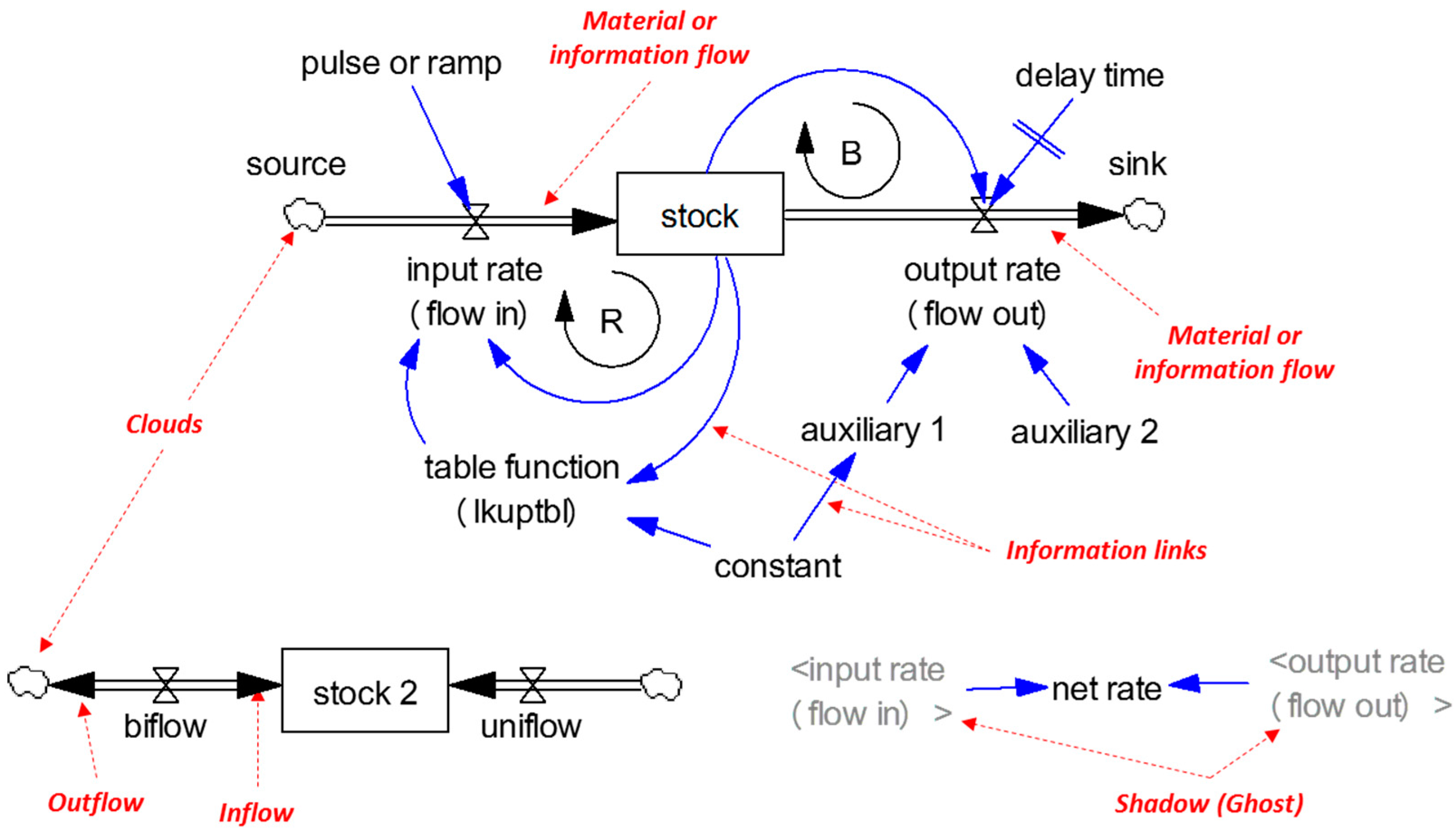
2. What Is System Dynamics (SD) Modeling Methodology?

The SD method was developed to enhance learning in complex systems, is fundamentally an interdisciplinary science (i.e., pertaining to more than one branch of knowledge; where two or more scientific disciplines are involved in a coordinated scientific investigation), is grounded in the theory of nonlinear dynamics and feedback control, and draws on cognitive and social psychology, economics, and other social sciences to incorporate human dimensions and decision making [33].
There are five general steps (similar to many other modeling approaches) used in applying the SD modeling process: (1) problem articulation; (2) development of a dynamic hypothesis; (3) formulation of a simulation model; (4) testing the simulation model; and (5) policy or strategy design, experimentation, and analysis (Table 1) [33]. The first step describes the researchers’ intentional effort to “admire the problem” rather than jumping to conclusions about the underlying mechanisms perpetuating an issue [34]. This may be achieved through stakeholder interviews or surveys, focus groups, eliciting mental models of the problem from key personnel, as well as collecting or aggregating all the relevant data that can describe the behavior of the problem over time (i.e., a reference mode). The second step aims to synthesize all that is known about the problem into an endogenous (i.e., feedback-based) theory upon which to evaluate the quantitative model (step 3). These first two steps are often associated or compared to “soft systems” methodology due to the emphasis placed on stakeholder engagement, defining decision-making criteria and mental models of the system actors/stakeholders, and conceptual modeling of the root causes of the problem of interest [33,34,35].
The third step is the construction of the quantitative model. Construction is aided by icon-based programming (consisting of stocks, flows, auxiliaries, information links, and clouds; Figure 1) used to conceptualize the primary feedback mechanisms and describe them using coupled partial differential equations. Practitioners advise modelers just setting out to “challenge the clouds” (clouds representing the boundaries of the quantitative model) by expanding their own mental and conceptual models about the problem at hand and resisting temptations to reduce the number of components included in the model for the sake of simplicity alone [36]. The fourth step attempts to “break” the model (i.e., test the model with extreme conditions and/or parameter values far outside the calibrated values which closely correspond to values in the real world) to investigate if assumed parameter values are realistic, if the direction of model responses correspond to expected feedback polarity to check model consistency, and to identify variables that could break the system or improve system function (e.g., potential leverage points) [33,37]. The third and fourth steps are often compared to “hard systems” methodology used in other types of systems analyses due to the emphasis placed on specifying system equations, objectives, constraints, ensuring basic natural laws are respected, and testing the model to understand its change in behavior quantitatively [33,37,38]. Interdisciplinary science is built into the SD methodology by the integration of both “soft” and “hard” components of a system or problem. The final step involves asking and applying “What if?” questions to the model based on proposed strategy or policy interventions (e.g., “what if government subsidies are raised or lowered?”; “what if different management practices are implemented?”) to identify places of management leverage or potential, and future tipping points. This summarizes the basic SD process behind the real-world applications described below. For methodological considerations of SD applied to different disciplines, see [39,40,41,42,43,44,45].

3. Application of System Dynamics to Agriculture and Natural Resource Problems

Before proceeding to the contemporary cases we have reviewed, it is important to acknowledge the first SD model incorporating AGNR relationships, which was the pioneering work of the World3 model published in The Limits to Growth in 1972 ([46]; updated in 1991 and 2004 [47,48]). The World3 model explored the upper limits of human developmental capacity by modeling the interacting feedback loops among five factors: population growth, food per capita production, nonrenewable resource depletion, industrial output, and pollution generation. Food production was considered one of the main drivers of population growth and was limited by reduced land fertility caused by pollution, which in turn was driven by population growth. The model assumed that higher food demand would cause higher land (arable) allocation to food production, thereby representing a limit to human population growth, and food production increases would cease due to land degradation when the arable land reaches its maximum level. Scenarios run with the World3 model resulted in overshoot and collapse of the human population in the mid-21st century due to the depletion of natural resources. The authors were largely criticized both for the novelty and uncertainty of the model and were labeled “pessimistic.” However, a recent comparison of the observed world data from 1970 to 2000 with the original estimates performed by [46] showed that historical data match favorably with the modeled trends [49,50,51].
Having summarized some persistent agriculture and natural resource (AGNR) problems and given an overview of the system dynamics (SD) modeling methodology (including the seminal work in The Limits to Growth study), this section reviews the application of SD to some contemporary AGNR problems, including hydrology and water resources; agriculture, land and soil resources; food system resiliency; and small holder development. Of the case studies presented, many involved stakeholder outreach and participation. Such activities were outside the scope of this review. Here we focus primarily on the integration of multiple scientific disciplines through the use of SD modeling. Although brief, each section directs the reader to multiple relevant resources that provide more detailed descriptions of the work described.

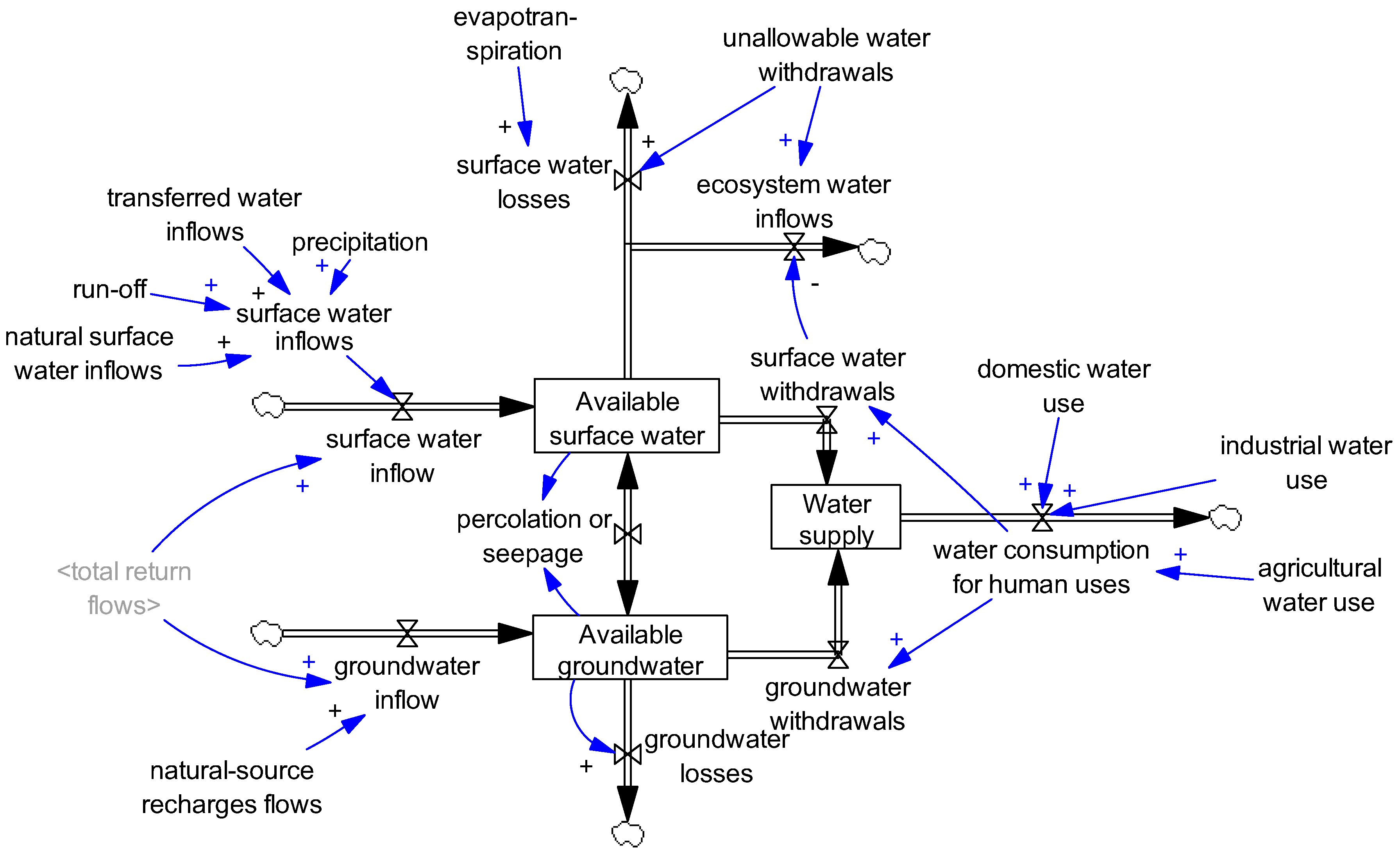
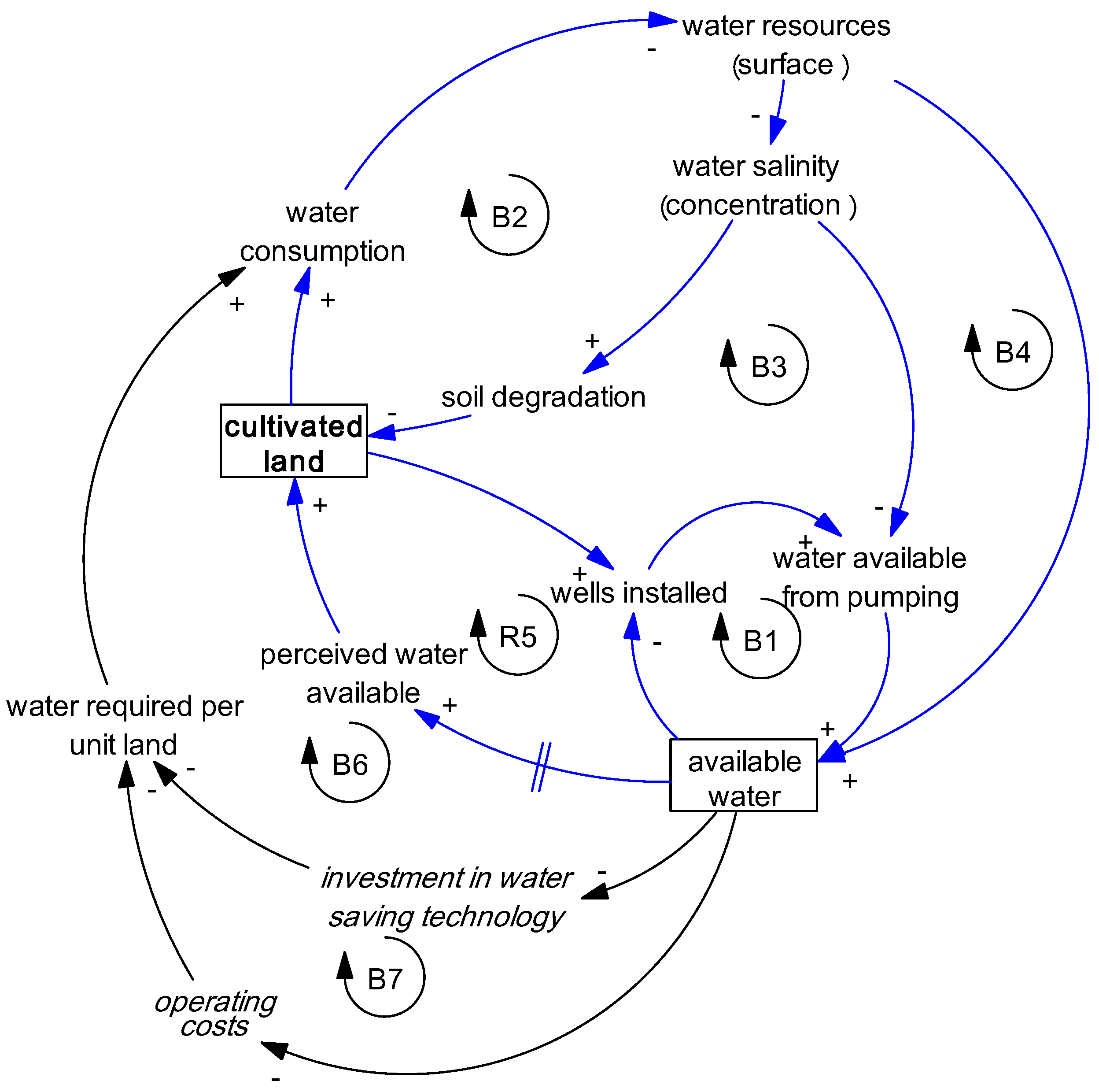
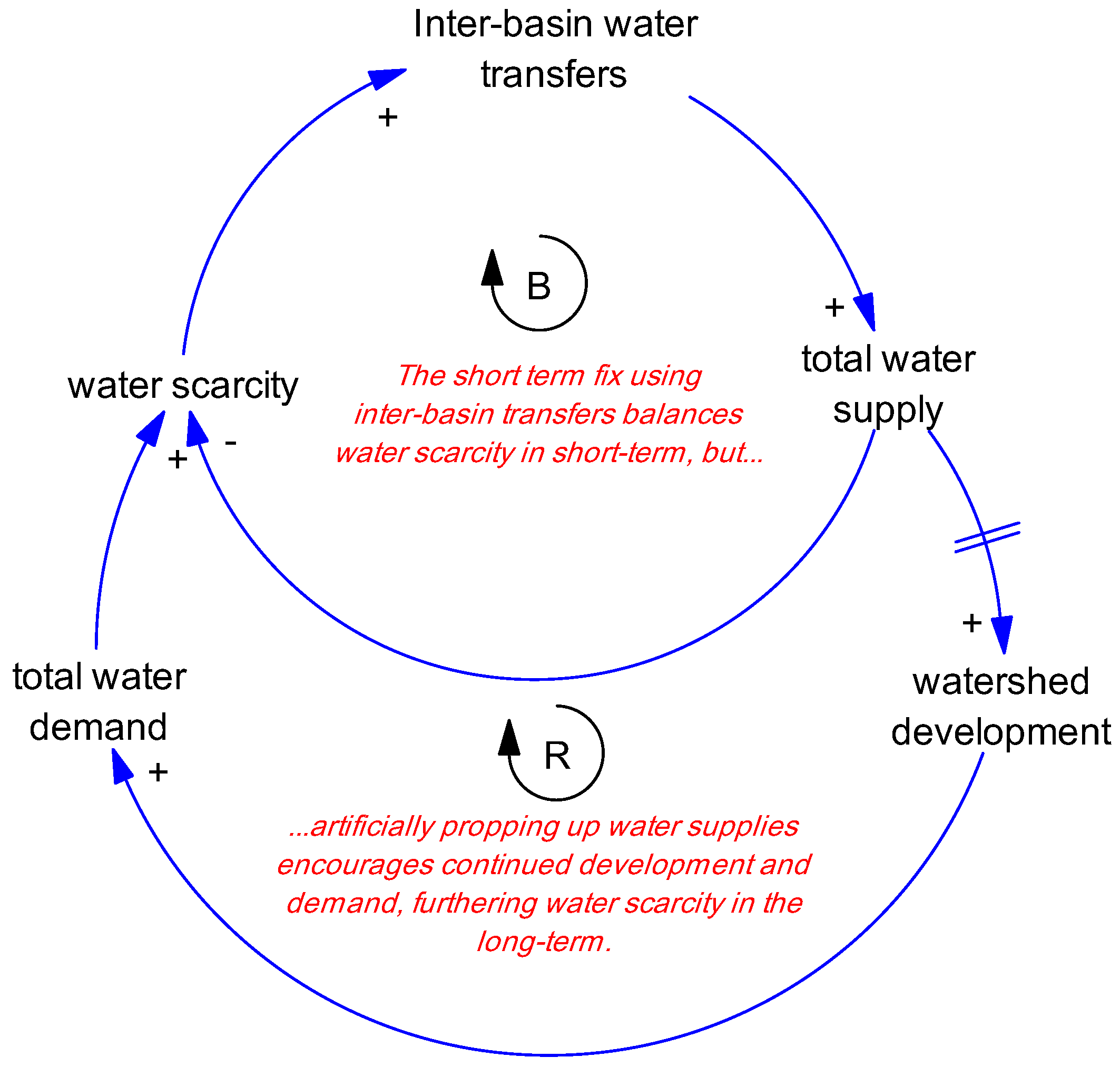
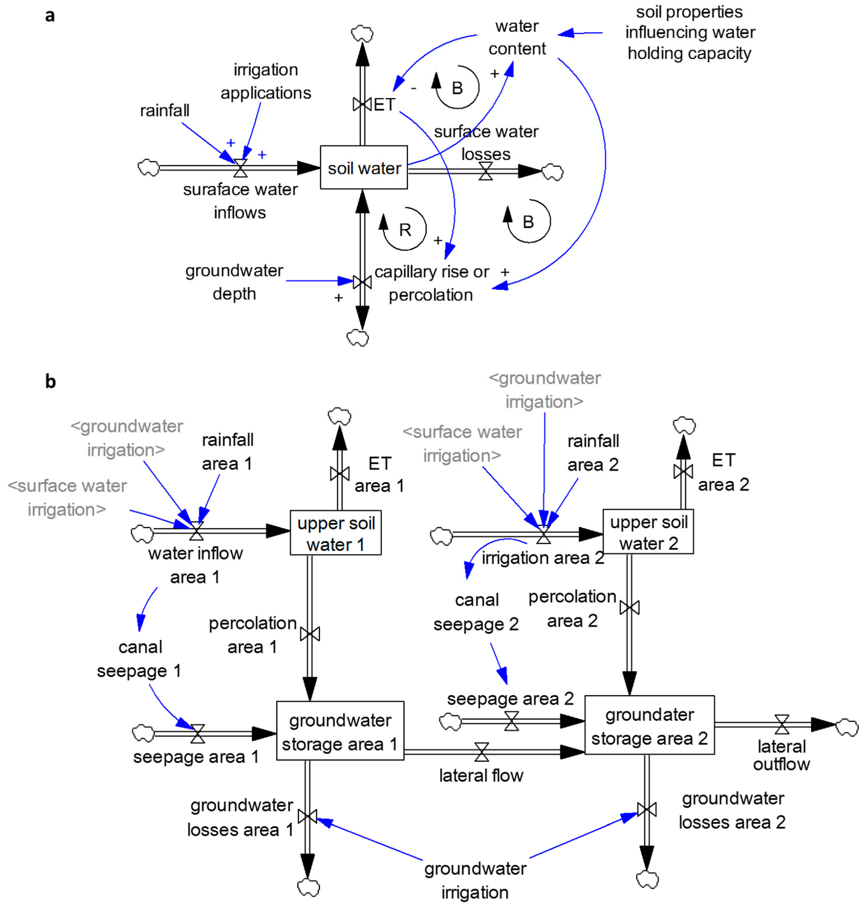
3.1. Hydrology and Water Resource Management

Hydrology and water resource management issues are inherently complex due to local climate characteristics (including variability in rainfall distribution patterns), surface water-groundwater connectivity, natural and man-made reservoir storage, growing populations and demand, among other factors. These characteristics make hydrologic and water resource management problems well suited to study by SD methodology. Scientists have used SD to study such problems beginning as the early as the 1980s with applications on small-scale hydropower analyses [51]. Various SD applications in hydrologic and water resource management problems can generally be categorized into two types: (1) water resource or watershed planning problems (where the research is used to better understand the current situation and/or to inform stakeholders regarding the current state of the system); and (2) scenario analyses of the impacts economics or policies have on water resources (i.e., to explore the behavior space of the current system given changed conditions or alternative strategies). In real-world situations, planning and analysis activities are often performed in tandem (i.e., one activity informs the other—a feedback loop in decisions and results) since they are each a respective step in the resource management process. In the literature, however, articles often focus on one activity or the other. Below, we provide some citations of each use (planning or analysis) with some illustrative applications.
Because of the integrative abilities of the SD method to connect physical and social system components, the emphasis on stakeholder participation, as well as the visual attractiveness of SD models, SD has been an effective tool for water resource planning problems throughout the world. There are many examples, both peer-reviewed [52,53,54,55,56,57,58] or presented at conferences [59,60,61]. Two illustrative cases dealing with groundwater management planning are shown, one in the Tenggeli Desert region, China, using qualitative causal loop diagramming [62], and another in the Palouse region, USA, which created a quantitative model to estimate groundwater drawdown rates useful for regional water planning and management [63].
Water resource planning case 1 Yaoba Oasis, China: Yaoba Oasis is an artificial oasis developed in the 1960s to resettle displaced herdsmen (“ecological refugees”) and relieve pressure from stressed grasslands [62]. Due to the arid environment, groundwater was pumped to support irrigation of newly cultivated land (Figure 2, loop 1). By doing so, aquifer levels were lowered, allowing salt water from the underground Taosuhu Lake to flow into the aquifer as water tables were lowered. Increased water salinity has degraded soils and limited the expansion of cultivated land (Figure 2, loop 2) as well as usable irrigation water (loop 3). As water wells are discarded due to salinity issues, water tables can recover and reduce salinity issues (loop 4). However, due to the delay in management perceptions of water availability, cultivated land continues to grow despite ongoing salinity concerns and a depleting water supply (loop 5). This behavior mimics both “fixes that backfire” (Figure 2) and “tragedy of the commons” archetypes [25,64]. Several contributing policies (subsidized water resource fees to reduce costs of crop production) as well as interventions (encouraging water-saving crops; investments in irrigation technology and well management, and institutional strengthening; loops 6 and 7) were identified. The addition of such strategies into the feedback loop structure highlighted potentially important leverage points for stakeholders regarding mechanisms to balance water consumption with water availability; similar situations of water resource constraints and strategies have been occurring globally.
Water resource planning case 2 The Palouse, USA: The Palouse region in Washington and Idaho, USA, has a growing rural population that is dependent on groundwater, relying on two basalt aquifers for potable water [63]. By synthesizing existing water resources data, researchers developed an SD model to simulate the Palouse hydrologic cycle and project trends in aquifer characteristics assuming that the current infrastructure does not change. By integrating population dynamics and hydrological processes at the surface with the geologic characteristics of the region, they found, in the near future, groundwater withdrawals will likely exceed recharge rates, making maintenance of groundwater resources unsustainable [63]. Another important result was identification of uncertainty in key system components (e.g., storativity and recharge) which are not readily affected by groundwater management efforts. This was a major contribution to the water resource planning effort since a better understanding of the behaviors of inflows and outflows of the aquifer helped inform stakeholders about managing the water resource. For additional material regarding systems thinking applied to water resource planning, see [65].
Similar to SD applications in water resource planning, water resource problem analyses (i.e., testing changing conditions or alternative policies) have had widespread application in the literature [55,66,67,68,69,70,71,72,73,74,75] as well as in the System Dynamics Society [76,77,78,79,80,81] across a broad range of issues from energy production to agriculture to municipal water management. We highlight two cases, one dealing with sensitivity analyses of uncertain socioeconomic parameters in a traditional irrigation community in northern New Mexico, USA [75], and another on scenario analyses of alternative water transfer policies in the Zayandeh-Rud River Basin of Iran [72].
Water resource analysis case 1 New Mexico, USA: Historic irrigation communities in northern New Mexico, USA (known as “acequias”) provide an array of ecosystem and socioeconomic goods and services based on the mechanisms of water distribution and management along hand-dug canals supplied by mountain snowmelt runoff. An SD model was developed to integrate information regarding community leadership, local hydrology, and agricultural economics. The researchers then tested (via scenario and sensitivity analyses) the extent to which community resource management practices centering on shared resources (e.g., water for floodplain irrigation) and community mutualism (i.e., shared responsibility of residents to maintain irrigation policies and cultural traditions) influenced the irrigation system function and ecosystem goods and services [75]. Similar to [63], the model revealed uncertainty in numerous system components, which the researchers explored through comprehensive sensitivity analyses. Sensitivity analyses revealed that agricultural profitability, community make-up (i.e., percentage of residents with historical familial ties), and land use (residential vs. cultivated) were key determinants of irrigation system response. This was due to their influence on feedback processes responding to input parameter perturbations [75]. Their results correspond well with other types of system analysis efforts in the field of socio-hydrology [82].
Water resource analysis case 2 Zayandeh-Rud River Basin, Iran: The Zayandeh-Rud River Basin has traditionally used a supply-chain oriented approach to deal with water stress in the past 60 years [72]. Researchers integrated the basin hydrologic, socioeconomic, and agricultural sub-systems (e.g., the hydrology sub-system, Figure 3) and tested alternative policy options for managing water stress, including business as usual (BAU; basin transfers assumed constant; ag water use efficiency = 45%), agricultural water demand management I, II, and III (AWDM; basin transfers similar to BAU but with different cropping patterns of 80% or 45% water use efficiency), and inter-basin water transfer with and without demand management (IBWT; representing transfers with or without groundwater pumping and improvements in agricultural water use efficiency). Forecasts for each of the policy scenario tests revealed divergent dynamics between the BAU scenario (increasing water shortages) and the AWD and IBWT strategies (consistent or decreasing water shortages). Their results indicated that common policy options for managing water shortages (primarily inter-basin transfers) promoted the growth of the system, and therefore, water demand, further perpetuating water shortage problems. Without considering the dynamics of the interrelated problems (i.e., the connections between hydrology, socioeconomics, and agriculture), water managers are bound to succumb to recurring and more severe water shortage problems. Management “quick-fix” strategies that are often employed (e.g., water transfers) are diagnosed by a common SD archetype (a commonly occurring systemic structure observed across numerous management situations) called “fixes that backfire” [25]. Overcoming this phenomenon requires a shift from short-term to long-term thinking (Figure 4) [25].

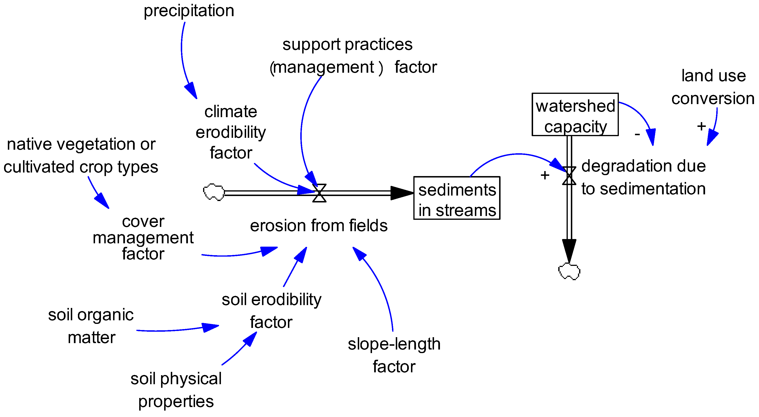
3.2. Agricultural Land and Soil Resources

As global populations continue to grow and more land becomes devoted to agriculture, agricultural production will have to be sustained on lands and soils traditionally not rated for intensive or long-term cultivation [11,16,17,19], creating elevated risk of soil erosion and other environmental externalities resulting from agricultural production [11,22,83]. Land use and agricultural practices may vary widely and can change based on modifications in public policies, pressure from urban expansion, changing economic conditions and profitability, and personal and cultural characteristics, among other factors. Because of the variety of influences, SD provides a useful framework for investigating how these socioeconomic characteristics influence the sustainability of land and soil resources, including both their productivity and ecosystem goods and services [84,85,86]. Land and soil models identified by our review may be categorized as: (1) soil modeling at the field scale via horizons; and (2) land management and erosion prevention at the watershed scale. Soil models at the field scale have focused on nutrient management [87], infiltration and water-holding capacity useful for reclamation decisions [88], or soil-water interactions useful for managing irrigation application for improved water use efficiency, reduced salinity, and reduced costs [89]. Likewise, several modeling efforts have documented the development, evaluation, and application of SD models representing reconstructed watersheds [90,91,92], which have been used to test and corroborate the implemented reclamation strategies within certain ranges of hydrologic conditions as well as compare different vegetation alternative for future reclaimed covers. Here, we highlight three illustrative SD applications, one at the soil layer scale, and two at the watershed scale.
Soil management at the soil layer scale with groundwater interactions: Due to the complex nature of water behavior in soils, managing irrigation water can be challenging due to common unintended consequences, including soil salinity issues as well as water table reductions due to reliance on pumping. In order to better understand the complex (nonlinear) interdependent relationships throughout the soil profile affecting soil water storage and the agricultural system, researchers developed a two-part SD model of soil-water-plant relationships with a dynamic link for interactions with the shallow groundwater table to account for natural recharge as well as pumping [89]. The surface layer model (Figure 5a) consisted of two balancing loops (ET → soil water content drawdown → reduction in ET; water content increase → percolation → reduction in soil water at surface) and one reinforcing loop (ET → capillary rise → soil water content → ET) around the soil water stock, while the surface-ground water interaction incorporated seepage, percolation, and lateral flows (Figure 5b). The model was then used to understand supplemental irrigation in aerobic rice systems, and demonstrated various water table drawdowns depending on irrigation application and groundwater abstraction rates. Because maintaining a sustainable groundwater resource is critical to sustainability, increasing irrigation applications can result in a “fix that backfires,” since continued irrigation applications may draw down the water table to the point that maintaining irrigation is too costly for the agricultural system.
Land management and soil erosion case 1 Alqueva, Portugal: The first case studied erosion and sedimentation in the Alqueva dam watershed, an agriculturally dominated area in southern Portugal [93]. The model used the Revised Universal Soil Loss Equation (RUSLE; [94]), which involves complex equations and large quantities of data. SD enabled the authors to circumvent this challenge by using the structural concepts of RUSLE and account for their interconnections while still generating meaningful predictions of soil erosion and sediment deposition at the watershed level (Figure 6). Their findings indicated erosion rates of 2.5–249.4 tons/ha. To aid in the improvement of agriculture practices utilized by farmers in the watershed, the model also identified the most influential factors on soil erosion given the particular soils in the watershed, aiding efforts to prevent soil loss and maximize capital for soil erosion prevention and remediation efforts.
Land management and soil erosion case 2 Keelung River, Taiwan: The second soil erosion case evaluated soil erosion and nutrient impact using an SD model in the Keelung watershed, one of Taiwan’s largest rivers which runs through the capital city Taipei [95]. For two decades prior to the study, Taipei’s urban and agriculture expansion had encroached on areas with steep slopes making the soils increasingly susceptible to erosion. Using a modified version of the generalized Watershed Loading Function [96], they estimated daily erosion up to 18,000 tons/day. Perhaps more importantly, the model captured the complexity of the problem by accounting for feedback between erosion, runoff, sediment, and economic (policy) sub-models. The economic component included subsidies to mitigate environmental risks, including afforestation subsidies, which reduced soil-related damage compared to the status quo. The approach the researchers developed offered a unique interface and data integration to conduct policy analyses for complex AGNR problems (Figure 7), allowing integration of other common computing platforms with SD. It is likely that advancements in Python™ and Statistical Program R [97] will continue to improve GIS integration into SD models.

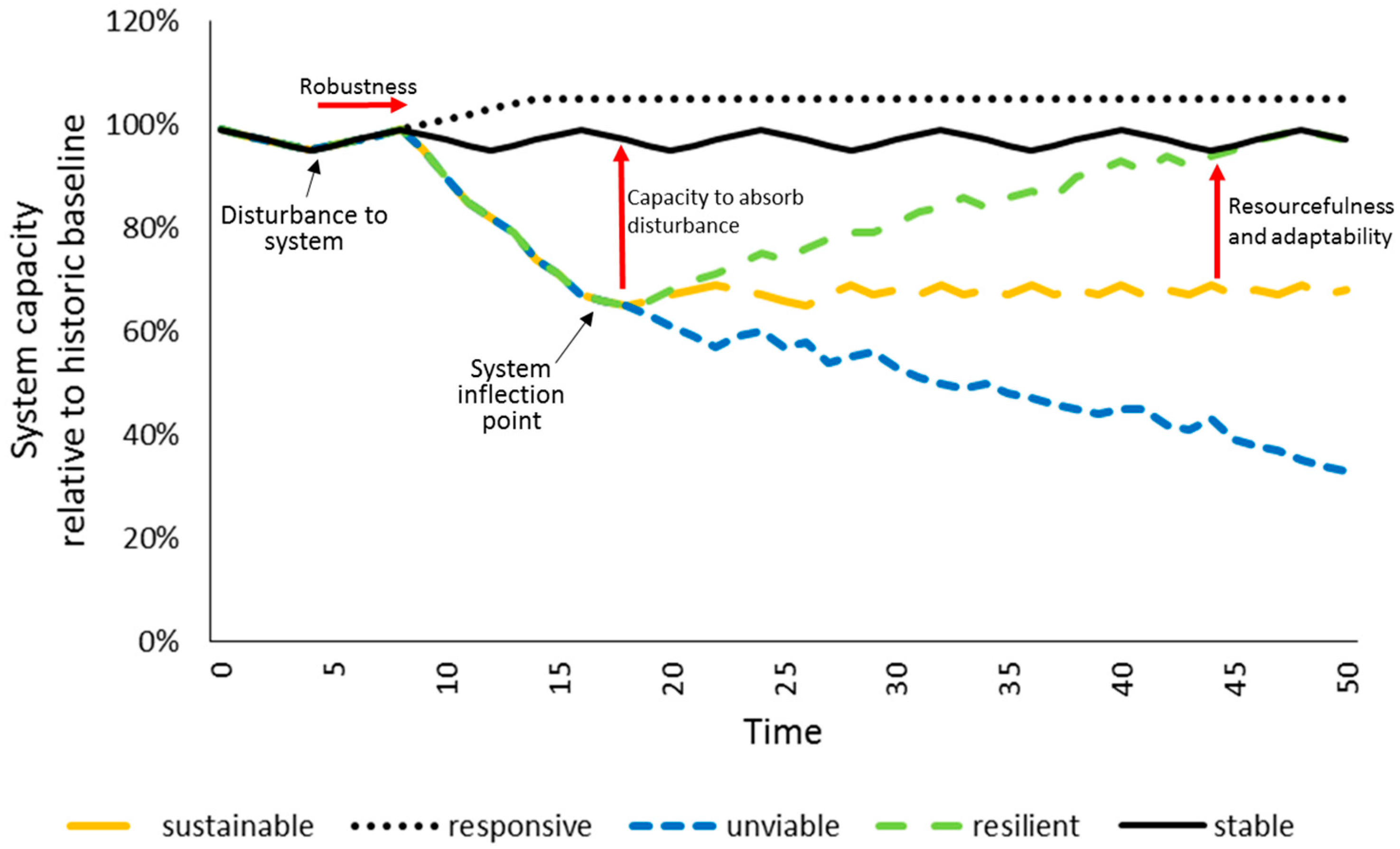
3.3. Food System Resiliency

From food to food systems: World population increase in the 20th century and ongoing challenges of under- or malnourished populations has increased global food insecurity trends and therefore pressure on food security (i.e., all people at all times have physical and economic access to sufficient and nutritious food to meet their needs for an active life [98]) provided by food systems (i.e., the set of activities from production to consumption, including geographic, biophysical, human and socioeconomic features, and environmental constraints [99]). Since then, models of single food-related variables have been used to predict future outcomes and support territorial food security policies. In particular, food production and consumption and partial indicators of food security are often used to deduce implications of future trends [100] or by performing descriptive flow analysis [101]. On the other hand, focus on food-related boundaries continue to change from those in the last century as society moves from food products to food systems. Others have compared the main features of modern food systems to traditional food systems showing that the modern transformation may be attributed to: increases in urban populations relative to rural populations; increased number of national and global stakeholders of food production relative to local agents; enhancement of the processing phases of the food system relative to production phases; and affirmation of the long-supply chains relative to shorter or more local supply chains [102].
The main factors limiting the achievement of food security were traditionally linked to production shocks due to natural factors (i.e., climate trends such as poor rainfall). However, in modern food systems, food security has been more associated with variation in international prices, foreign trade problems, and income shocks causing food poverty [102]. It is now evident that food systems are affected by AGNR drivers but also produce outcomes in social capital (welfare, employment, wealth, etc.) and natural capital (environmental security, ecosystem services, stock variation, etc.) [93]. In response to these issues, food policies enacted by national ministries or departments of agriculture have switched from agricultural technology and production improvements to regulation around industrial competition, health and food safety, and waste management related to the food chains [99,102].
Other papers have reported insights to support food security policy at territorial and local levels. A non-exhaustive list of published models focusing on regional or local food systems was presented by [103]. SD models have focused on closing the food sufficiency gap. For example, in Colombia, food sufficiency is highly dependent on the land use and food demand, requiring a sustainable goal-seeking behavior of increasing producer training, service infrastructure, as well as adjustments in irrigation and drainage. Models have corroborated that increased productivity and efficiency will be required rather than agricultural land expansion [104]. Other uses of SD in food system research include food system distribution optimization for developing and transition countries [105] showing how food dynamics are deeply embedded in urban and rural dynamics and therefore the food systems cannot be managed as separate parts (e.g., urban versus rural; production versus retailing) [106,107,108].
To be sustainable, food policies have to be directed toward efficient AGNR management, including the supporting infrastructure of the food system (e.g., technology, organizational quality, roads, urban planning, etc.) and will have to be based on minimizing food gaps and maximizing food resilience. The pressure or temptation to lower food security and food system resiliency goals (e.g., 100% to 90% of food gaps closed by 2050) will be immense [107], leading to “drifting goals” behaviors among policymakers likely to support food resiliency for some albeit to the exclusion of others through the persistence of the food availability gap (Figure 8). The food availability gap varies due to two primary drivers: food demand (B1; which is the desired goal) and current food supplies provided by the system (B2; representing urban and rural resources) [106]. Rash policies directed towards infrastructure development in order to facilitate exchanges and food distribution (e.g., road building to generate greater accessibility) might be effective in the short-term but will incentivize continued urbanization, exacerbating congestion of the infrastructure and thereby eroding the ability to deliver food supplies, creating a “fix that backfires” (loops B2 and R3). Policies on resource use should account for natural limits to the system and respect the “limits to growth” (i.e., natural resources capacity; B2 and R4). In this context, it should be identified and emphasized that policies that degrade natural resource capacity (the carrying capacity of the system) might negatively affect food system production and increase the food gap. It indicates that food policy design should be oriented to maintain the system’s capacity to produce and distribute food, taking into account the current socioeconomic structures and the nation-state as a whole in order to support their human developmental capacity while respecting the natural constraints enforced by the local environmental and biophysical limits [108].
From food systems to food resilience: Systems perspectives of food systems that utilize holistic approaches such as SD (which focus on the relationships among the parts rather than the parts only [25,32]) can account for whole-system interactions and improve sustainability outcomes of food systems [109]. Internal and external drivers of change that appear as long-term pressures to the system can increase the system’s insecurity and exacerbate the problem of low food system resilience.
As described by [109], resilience thinking may assume different definitions depending on the area of application. The same authors reported that, in general, resilience is a dynamic concept that is broadly defined as the capacity of a system to continue to achieve goals despite disturbances and shocks [109]. This is an essential part of sustainability and might be measured by the system’s performance in the long run. Resilience is complementary to the concept of sustainability (e.g., the measure of the system performance in the long run) by measuring the capacity of the system to face disturbances. Therefore, food system resiliency was defined as “the capacity over time of a food system and its units at multiple levels, to provide sufficient, appropriate and accessible food to all, in the face of various and even unforeseen disturbances” [109]. A more resilient system can absorb a shock with a more rapid recovery than a less resilient one (Figure 9). Reduced resilience can cause incomplete system recovery resulting in sustainability albeit at an overall lower system capacity (similar behaviors are observed in the system archetype of drifting goals, where original standards are abandoned or forgotten in favor of short-term success or new, albeit lower, standards of resilience). Following the resilience action cycle approach, food resilience problems have been studied and analyzed with SD to develop viable solutions for sustainable economies, especially in developing countries [110,111,112,113]. To build resilience in food systems with aid from quantitative models, three different boundary-scale levels are recommended [109]: (1) national and regional on which territorial policies will be considered; (2) supply chain on which special products and value-chains are considered from local to global level, and (3) individual perspectives regarding smallholders and their livelihoods.

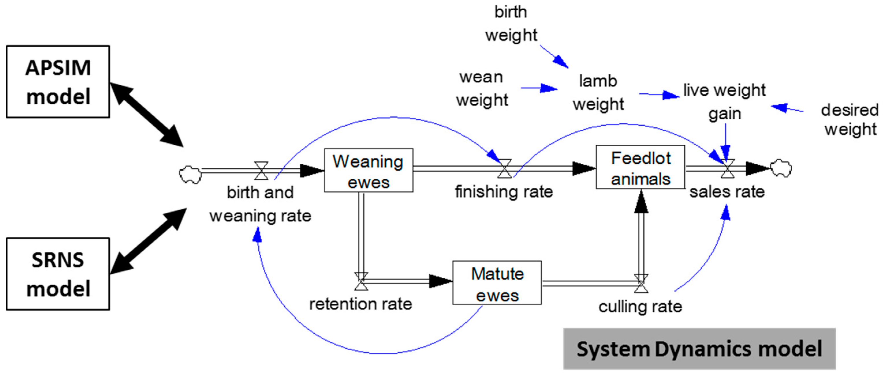
3.4. Integration of Smallholder Crop-Livestock Production and Smallholder Development

Sustainable intensification is a topic recently disseminated to solve social and economic inequalities around the world, and livestock is an intrinsic part of this sustainability enigma [114]. However, because of the complexity of the social-economic-environmental aspects of sustainability, system-oriented approaches for decision making are needed to succeed [24,115,116]. A holistic approach for integrating the crop-livestock-social components of sustainable intensification is required for effective deployment of technologies and assessment of failures. Many attempts in using decision support systems have been documented [114], but the application of SD in livestock is incipient [116]. Smallholder animal farmers are part of the sustainable livestock intensification program; mainly those in tropical regions that are mostly vulnerable to climate change [114]. The social aspect of smallholder crop-livestock production systems is extremely important because it entails subsistence farmers and herders, and small communities that are adapted to specific regions. SD models can be used to link social, economic, production, and environmental aspects because they rely on a big-picture perspective rather than being concerned with small details. For example, researchers have used an SD model to understand the functioning of mixed farming systems in the tropics, specifically in the Yucatán peninsula, including different components such as nutrition and management of sheep; partitioning of nutrients; flock dynamics; local and regional sheep production, marketing and economics; and labor [117]. A multi-objective modeling approach was adopted by combining different computer programs: the Agriculture Production Systems Simulator (APSIM) for crop modeling [118] and the Small Ruminant Nutrition System (SRNS) for animal modeling [119] with an SD model interfacing both programs (Figure 10). Applying their model to compare specialized systems versus mixed farming, they concluded the mixed farming scenario provided more income than specialized enterprises [120]. They suggested that for smallholders in that region, specialization was not sustainable, and therefore, mixed crop-livestock was the best production option.
Smallholders are considered the core of rural growth, especial in developing countries. Smallholders are often subsidence farmers that consider food security as the main objective and profit as the second objective [121]. SD models developed in the last decade were applied to describe rural communities and smallholder farm dynamics to support technical choices [121,122], promote rural growth and improve an efficient use of the AGNR [113,123,124], increase the technical training of farmers in rural communities of developing countries [125], and integrate smallholders in their socioeconomic and environmental context [126].

4. Discussion on the Roles of System Dynamics for Emergent Agriculture and Natural Resource Management Challenges

Based on the above cases, it is clear that SD has a role in addressing AGNR management problems. The role of SD in contemporary AGNR problems dates back to the earliest SD models, including World3 [46], and over the subsequent decades, SD has branched out into varying disciplines in order to account for greater specificity and complexity of the AGNR problems at hand. It is now evident that food systems are primarily affected by AGNR drivers. However, they also produce outcomes in social capital (welfare, employment, wealth, etc.) and natural capital (environmental security, ecosystem services, etc.) through feedback mechanisms between food consumer and producer sectors [99]. SD models have increased their focus on natural resource constraints that potentially limit the behavior of socioecological systems (e.g., food system infrastructure; growth of urban centers) (see [108]). We have highlighted several noteworthy cases of SD applied to water resources, land and soil, food systems, or smallholder livelihood issues. In each of these cases, the SD modeling method facilitated identification of key insights not previously recognized by researchers or practitioners in their respective disciplines. It follows from these cases that AGNR features and dynamics need to be included in future model boundaries of investigations around social and political stability, especially those where natural resources may be a component of the problem or conflict. Incorporating agricultural system resiliency measures into SD models will be useful if the aim is to find appropriate adaptation strategies to changing conditions in the long term [126].
Interestingly, several system archetypes were identified in a number of the case studies (e.g., fixes that backfire [62,65,89,106], Figure 2, Figure 4, and Figure 8; drifting goals [106,109,114], Figure 8 and Figure 9; limits to growth [106]; and tragedy of the commons [62]). The two most commonly identified archetypes were fixes that backfire and drifting goals. The generic fix that backfires situation is characterized by a “quick fix” to alleviate a problem (which works in the short term), but employing the fix creates unintended consequences that reinforce, or perpetuate, the original problem (i.e., the problem persists in the long term). The feedback loop structure is a balancing loop (the “quick fix”) embedded within a reinforcing loop (the unintended consequence). On the other hand, the drifting goals situation is characterized by the person, organization, or system that strives to meet a certain goal (e.g., a quality standard; profitability or production goal), but while waiting to see the results of invested efforts, it becomes easier to be satisfied with less and therefore lower the original goal [25]. The feedback loop structure of the drifting goals archetype is two connected balancing loops (one long-term loop capturing the invested effort to meet the original goal; one short-term loop that captures the pressure to lower the goal to a level that is easier to achieve).
Within SD modeling, archetypes are not unrelated [127,128]. We find that AGNR problems, based on the above cases, are on a path to falling into the common trap known as shifting the burden (Figure 11). The shifting the burden archetype is characterized by two balancing loops (similar to drifting goals) embedded within a reinforcing loop (similar to fixes that backfire). One loop captures a long-term solution to alleviate a chronic problem (e.g., meet societal needs for food and fiber production through regenerative solutions that protect biodiversity and enhance soil and water resources; B1 in Figure 11). Another loop captures the “quick-fix” solution (e.g., reliance on capitalizing easily attainable resources without regard for any social or environmental externalities; “take-make-waste” within B2 of Figure 11). The “quick fix” also represents lowering the overall sustainability goal (i.e., content with “take-make-waste” alternatives since they are generally faster and cheaper). The trap of shifting the burden lies in the unintended consequences (i.e., R loop in Figure 11), where reliance on short-term solutions are reinforced through unintended consequences on social systems (e.g., sunk costs which reduce management adaptability) and environmental systems (e.g., degraded ecosystems that lengthen restoration times and overall productivity). These short-term actions are often based on erroneous assumptions (e.g., infinite and cheap energy; non-limiting waste disposal capacity; non-limiting water and soil; stronger environmental resilience; etc.) [129]. In order to formulate effective policies that support fundamental solutions in the long term, supporting systemic perspectives and testing proposed strategies with tested models and scenarios of future behaviors will require collaborative approaches, where system researchers and stakeholders work together to identify and implement sustainable strategies [129,130]. Although our review has focused on examples of discipline integration through SD modeling, readers interested in stakeholder outreach and participation and how SD can provide aid in the decision-making process are encouraged to see [130].
Whether or not researchers fully adopt SD as their chosen methodology (and certainly not all scientists will become SD modelers in the sense they formulate models and test different policies), future approaches will increasingly become interdisciplinary in order to deal with the multifaceted and complex nature of AGNR problems. In such cases, the recognition and adoption of SD can hold great value, given it provides a proven modeling methodology to identify, describe, and quantitatively test the feedback loops interacting within a given system [33]. Even in most circumstances where not all of the interdisciplinary team members are SD modelers, they will still be integral to the research investigation due to their disciplinary expertise, which can enlighten researchers from other disciplines about the complexity of each respective component of the problem as well as inform the model formulation through the provision of expert knowledge (either personally or through guidance in the scientific literature) to the model developers.
Another unique capability that was observed in multiple case studies is that SD has the ability to connect and interface with other computer programs in a user-friendly manner. This makes SD a useful and necessary tool that should be integrated with different modeling platforms. Those platforms might be less adept at capturing feedback loop-driven processes and could offer different useful information such as data specialization in the case of GIS, agent behavior with agent-based modeling platforms, or input values to set up initial conditions in the case of empirical models specially developed for technical purposes. SD aids in “seeing the big picture” and with the array of SD programs, researchers now have a suite of model-building platforms that can integrate other types of models that otherwise could not be used in tandem.
A major limitation of the SD approach is the risk to formulating erroneous policies by trusting simulations of poor (i.e., unvalidated) models that produce inaccurate results (due to poor technical and evaluation considerations). The wide-ranging availability of modeling tools and software has made model development easier (particularly for novices without deep knowledge of biophysical or socioeconomic processes) and tempts modelers to quickly develop and test models without fully understanding the endogenous dynamics. Model critique and evaluation is critical before policy strategy recommendations are made. In order to build confidence in model results and recommendations, good modeling practices require (1) use of local knowledge and/or historical data to calibrate model predictions to reality; (2) sensitivity analyses of key variables (e.g., Monte Carlo simulation) and model boundary and extreme condition testing to gauge the model’s respect of physical and economic laws; and (3) analysis of scenarios compared to expert opinions (for model calibration and evaluation techniques, see [33,131,132]). Other limitations or criticisms of SD modeling include applications to the work type of problems, incorrectly applying the SD modeling method and its frameworks, and/or the tendency to build unnecessarily large models for “big” problems (for robust descriptions of these and other limitations as well as their handling strategies, see [133,134,135]). In this sense, SD modeling requires equal collaboration across boundaries [129]. For the scientific community, it will require increasing model building and model evaluation capacities, especially enhancing interdisciplinary approaches in modeling, as well as robust protocols of policy evaluation on the effects of applied actions on AGNR systems. Since all models are simplifications of reality and systems continually evolve, it is important that models are updated and improved as we learn more about the complex interrelationships contributing to the problems we face.
Finally, adoption of SD to a wider range of practitioners will remain difficult due to learning barriers observed in complex systems (e.g., limited information; confounding variables and ambiguity; misperceptions of feedback; flawed cognitive maps or (linear) mental models; defensive routines [136,137]). Overcoming these barriers requires improving the learning process (including primary and secondary education offerings in systems thinking), developing learning opportunities through management flight simulators (interactive computer models allowing participants to practice and learn dynamic decision making in real-time), reorganizing organizations to incentivize individuals to pursue systemic cause-and-effect solutions [136,137], and perhaps most importantly, overcoming deeply ingrained preconceptions by pausing to “admiring the problem” to assist in the shift from short-term to long-term thinking (Figure 11; [129]).

5. Conclusions

In this paper, we have described a variety of agriculture and natural resource management (AGNR) problems occurring globally. System dynamics (SD) provides a valuable framework for investigating these complex AGNR issues, specifically through the use of computer simulation modeling. After briefly describing the SD methodology, we provided an extensive review of SD applications to water, soil, food systems, and smallholder issues and illustrated in these cases several system archetype behaviors (e.g., fixes that backfire; drifting goals). Continuing down these paths are likely to lead to reliance upon short-term solutions to AGNR problems (i.e., “quick fixes” or “take-make-waste”), making it more difficult to employ fundamental solutions (e.g., regenerative solutions). If AGNR goals continue to “drift” (i.e., settle for lower sustainability goals regarding resource use and externalities), AGNR systems are likely to fall into the trap of “shifting the burden,” where reliance on “quick fixes” become the only feasible alternative. We conclude that common attempts to alleviate AGNR problems, across continents and regardless of the types of resources involved, have suffered from reliance on short-term management strategies. To effectively address AGNR problems, longer-term thinking and strategies aimed at fundamental solutions will be needed to better identify and minimize the often delayed, and unintended, consequences arising from feedback between management interventions and AGNR systems.
The ability of SD to aid in recognition of complex interacting factors and scientifically test different management or policy strategies was also of key importance. Several cases described ways in which SD was used to integrate with different types of models (e.g., RUSLE or APSIM) or computer applications (e.g., Microsoft Excel or ArcGIS), highlighting the potential that SD programs have to address complex AGNR issues by integrating different types of scientists and models into collaborative interdisciplinary investigations. However, adoption of SD into other disciplines remains slow due to a number of barriers, hindering more transformative or transdisciplinary research. Overcoming these barriers is possible and it will be essential to integrate concepts and models across a wide array of sciences in order to adequately address the emerging AGNR challenges. Due to the strengths embedded in SD methodology, SD provides a valuable framework to investigate AGNR problems, both independently and in tandem with other types of models and disciplines. SD should be a central tool for conducting transdisciplinary research capable of addressing our most pressing AGNR issues.

Acknowledgments

We’d like to thank two anonymous reviewers for their very helpful comments provided during the review process—both of which greatly improved the paper.

Author Contributions

B.T. organized the outline of the manuscript and Section 1 and Section 2. H.M., L.T., and A.A. constructed Section 3 and Section 4 and provided editorial comments throughout the entire manuscript. R.G. constructed the conclusions and abstract and provided editorial comments and direction throughout the development of the manuscript.

Conflicts of Interest

The authors declare no conflict of interest.

References

  1. Trenberth, K.E.; Dai, A.; van der Schrier, G.; Jones, P.D.; Barinchivich, J.; Briffa, K.R.; Sheffield, J. Global warming and changes in drought. Nat. Clim. Chang. 2013, 4, 17–22. [Google Scholar] [CrossRef]
  2. Akerlof, K.; Maiback, E.W.; Fitzgerald, D.; Cedeno, A.Y.; Neuman, A. Do people “personally experience” global warming, and if so how, and does it matter? Glob. Environ. Chang. 2012. [Google Scholar] [CrossRef]
  3. Corlett, R.T.; Westcott, D.A. Will plant movements keep up with climate change? Trends Ecol. Evol. 2013. [Google Scholar] [CrossRef] [PubMed]
  4. Sheffield, J.; Wood, E.F.; Roderick, M.I. Little change in global drought over the past 60 years. Nature 2012, 491, 435–438. [Google Scholar] [CrossRef] [PubMed]
  5. Taylor, R.G.; Scanlan, B.; Doll, P.; Rodell, M.; van Beek, R.; Wada, Y.; Longuevergne, L.; Leblanc, M.; Famiglietti, J.S.; Edmunds, M.; et al. Groundwater and climate change. Nat. Clim. Chang. 2012. [Google Scholar] [CrossRef] [Green Version]
  6. Haddeland, I.; Heinke, J.; Biemans, H.; Eisner, S.; Florke, M.; Hanasaki, N.; Konzmann, M.; Ludwig, F.; Masald, Y.; Schewe, J.; et al. Global water resources affected by human interventions and climate change. PNAS 2014, 111, 3251–3256. [Google Scholar] [CrossRef] [PubMed]
  7. Walsh, C.L.; Blenkinsop, S.; Fowler, H.J.; Burton, A.; Dawson, R.J.; Glenis, V.; Manning, L.J.; Kilsby, C.G. Adaptation of water resource systems to an uncertain future. Hydrol. Earth Syst. Sci. Discuss. 2015, 12, 8853–8889. [Google Scholar] [CrossRef]
  8. Savenige, H.H.G.; Hoekstra, A.Y.; van der Zaag, P. Evolving water science in the Anthropocene. Hydrol. Earth Syst. Sci. 2014, 18, 319–332. [Google Scholar] [CrossRef]
  9. Mahmood, R.; Pielke, R.A., Sr.; Hubbard, K.G.; Niyogi, D.; Dirmeyer, P.A.; McAlpine, C.; Carleton, A.M.; Hale, R.; Gameda, S.; Beltran-Przekurat, A.; et al. Land cover changes and their biogeophysical effects on climate. Int. J. Climatol. 2014, 34, 929–953. [Google Scholar] [CrossRef]
  10. Seto, K.C.; Gueralp, B.; Hutyra, L.R. Global forecasts of urban expansion to 2030 and direct impacts on biodiversity and carbon pools. PNAS 2012, 109, 16083–16088. [Google Scholar] [CrossRef] [PubMed]
  11. Van den Bergh, J.C.J.M.; Grazi, F. Ecological footprint policy? Land use as an environmental indicator. J. Ind. Ecol. 2013. [Google Scholar] [CrossRef]
  12. Nepstad, D.C.; Boyd, W.; Stickler, C.M.; Bezerra, T.; Azevedo, A. Responding to climate change and the global land crisis: REDD+, market transformation and low emissions rural development. Philos. Trans. R. Soc. B 2013. [Google Scholar] [CrossRef] [PubMed]
  13. Bellard, C.; Bertelsmeier, C.; Leadley, P.; Thuiller, W.; Courchamp, F. Impacts of climate change on the future of biodiversity. Ecol. Lett. 2012, 15, 365–377. [Google Scholar] [CrossRef] [PubMed]
  14. Cheung, W.W.L.; Sarmiento, J.L.; Dunne, J.; Frolicher, T.L.; Lam, V.W.Y.; Deng Palomares, M.L.; Watson, R.; Pauly, D. Shrinking of fishes exacerbates impacts of global ocean changes on marine ecosystems. Nat. Clim. Chang. 2012. [Google Scholar] [CrossRef]
  15. Pauls, S.U.; Nowak, C.; Balint, M.; Pfenninger, M. The impact of global climate change on genetic diversity within populations and species. Mol. Ecol. 2013, 22, 925–946. [Google Scholar] [CrossRef] [PubMed]
  16. Wheeler, T.; von Braun, J. Climate Change Impacts on Global Food Security. Science 2013, 341, 508–513. [Google Scholar] [CrossRef] [PubMed]
  17. Van Ittersum, M.K.; Cassman, K.G.; Grassini, P.; Wolf, J.; Tittonell, P.; Hochman, Z. Yield gap analysis with local to global relevance—A review. Field Crops Res. 2013, 143, 4–17. [Google Scholar] [CrossRef]
  18. Vermeulen, S.J.; Campbell, B.M.; Ingram, J.S.I. Climate Change and Food Systems. Annu. Rev. Environ. Resour. 2012, 37, 195–222. [Google Scholar] [CrossRef]
  19. Teixeira, E.I.; Fischer, G.; van Velthuizen, H.; Walter, C.; Ewert, F. Global hot-spots of heat stress on agricultural crops due to climate change. Agric. For. Meteorol. 2013, 170, 206–215. [Google Scholar] [CrossRef]
  20. Shindell, D.; Kuylenstierna, J.C.I.; Vignati, E.; van Dingene, R.; Amann, M.; Klimont, Z.; Anenberg, S.C.; Muller, N.; Janssens-Maenhout, G.; Raes, F.; et al. Simultaneously mitigating near-term climate change and improving human health and food security. Science 2012, 335. [Google Scholar] [CrossRef] [PubMed]
  21. Bommarco, R.; Kleijn, D.; Potts, S.G. Ecological intensification: Harnessing ecosystem services for food security. Trends Ecol. Evol. 2012. [Google Scholar] [CrossRef] [PubMed]
  22. Garnett, T.; Appleby, M.C.; Balmford, A.; Bateman, I.J.; Benton, T.G.; Bloomer, P.; Burlingame, B.; Dawkins, M.; Dolan, L.; Fraser, D.; et al. Sustainable intensification in agriculture: Premises and policies. Science 2013, 341, 33–34. [Google Scholar] [CrossRef] [PubMed] [Green Version]
  23. West, P.C.; Gerber, J.S.; Engstrom, P.M.; Mueller, N.D.; Brauman, K.A.; Carlson, K.M.; Cassidy, E.S.; Johnston, M.; MacDonald, G.K.; Ray, D.K.; et al. Leverage points for improving global food security and the environment. Science 2014, 345, 325–328. [Google Scholar] [CrossRef] [PubMed]
  24. Liu, J.; Mooney, H.; Hull, V.; Davis, S.J.; Gaskell, J.; Hertel, T.; Lubchenco, J.; Seto, K.C.; Gleick, P.; Kremen, C.; et al. Systems integration and global sustainability. Science 2015, 347. [Google Scholar] [CrossRef] [PubMed]
  25. Senge, P.M. The Fifth Discipline, 1st ed.; Doubleday: New York, NY, USA, 1990. [Google Scholar]
  26. Cilliers, P.; Biggs, H.C.; Blignaut, S.; Choles, A.G.; Hofmeyr, J.-H.S.; Jewitt, G.P.W.; Roux, D.J. Complexity, modeling, and natural resource management. Ecol. Soc. 2013, 18, 1. [Google Scholar] [CrossRef]
  27. Doyle, J.K.; Ford, D.N. Mental Models Concepts for system dynamics research. Syst. Dyn. Rev. 1998, 14, 3–29. [Google Scholar] [CrossRef]
  28. Forrester, J.W. The “model versus a modeling process”. Syst. Dyn. Rev. 1985, 1, 133–134. [Google Scholar] [CrossRef]
  29. Beautement, P.; Broenner, C. Complexity Demystified: A Guide for Practitioners; Triarchy Press: Devon, UK, 2011. [Google Scholar]
  30. Bawden, R.J. Systems Thinking and Practice in Agriculture. J. Dairy Sci. 1991, 74, 2362–2373. [Google Scholar] [CrossRef]
  31. Dahlberg, K. Beyond the Green Revolution, 1st ed.; Plenum Press: New York, NY, USA, 1979. [Google Scholar]
  32. Stirzaker, R.; Biggs, H.; Roux, D.; Cilliers, P. Requisite simplicities to help negotiate complex problems. Ambio 2010, 39, 600–607. [Google Scholar] [CrossRef] [PubMed]
  33. Sterman, J.D. Business Dynamics, 1st ed.; Irwin McGraw-Hill: New York, NY, USA, 2000. [Google Scholar]
  34. Goodman, M. “Everyone’s Problem to Solve: Systems Thinking Cross-Functionally”. The Systems Thinker Newsletter, June/July 2006. Available online: https://thesystemsthinker.com/everyones-problem-to-solve-systems-thinking-cross-functionally/ (accessed on 14 September 2016).
  35. Lane, D.C. Should System Dynamics be Described as a ‘Hard’ or ‘Deterministic’ Systems Approach? Syst. Res. Behav. Sci. 2000, 17, 3–22. [Google Scholar] [CrossRef]
  36. Richmond, B. An Introduction to Systems Thinking, STELLA, 3rd ed.; High Performance Systems, Inc.: Lebanon, NH, USA, 2001. [Google Scholar]
  37. Miller, J. Active nonlinear tests (ANTs) of complex simulation models. Manag. Sci. 1998, 44, 820–830. [Google Scholar] [CrossRef]
  38. Checkland, P.; Holwell, S. “Classic” OR and “soft” OR—An asymmetric complementarity. In Systems Modeling: Theory and Practice; Pidd, M., Ed.; John Wiley & Sons, Inc.: Chichester, UK, 2004. [Google Scholar]
  39. Ford, A. Modeling the Environment, 1st ed.; Island Press: Washington, DC, USA, 1999. [Google Scholar]
  40. Deaton, M.I.; Winebrake, J.J. Dynamic Modeling of Environmental Systems, 1st ed.; Springer: New York, NY, USA, 2000. [Google Scholar]
  41. Grant, W.E.; Pedersen, E.K.; Marin, S.L. Ecology and Natural Resource Management Systems Analysis and Simulation, 1st ed.; John Wiley and Sons, Inc.: New York, NY, USA, 1997. [Google Scholar]
  42. McGarvey, B.; Hannon, B. Dynamic Modeling for Business Management, 1st ed.; Springer: New York, NY, USA, 2004. [Google Scholar]
  43. Ruth, M.; Hannon, B. Model Dynamic Economic Systems; Springer: New York, NY, USA, 1997. [Google Scholar]
  44. Hannon, B.; Ruth, M. Modeling Dynamic Biological Systems; Springer: New York, NY, USA, 1997. [Google Scholar]
  45. Costanza, R.; Voinov, A. Landscape Simulation Modeling; Springer: New York, NY, USA, 2004. [Google Scholar]
  46. Meadows, D.; Randers, J.; Meadows, D.; Behrens, W.W. The Limits to Growth; Universe Books: New York, NY, USA, 1972. [Google Scholar]
  47. Meadows, D.H.; Meadows, D.L.; Randers, J. Beyond the Limits; Chelsey Green: Post Mills, VT, USA, 1992. [Google Scholar]
  48. Meadows, D.H.; Randers, J.; Meadows, D.L. Limits to Growth—The 30-Year Update; Chelsea Green: White River Junction, VT, USA, 2004. [Google Scholar]
  49. Turner, G. A comparison of the Limits to Growth with 30 years of reality. Glob. Environ. Chang. 2008, 18, 397–411. [Google Scholar] [CrossRef]
  50. Meadows, D.L. Evaluating past forecasts: Reflections on one critique of The Limits to Growth. In Sustainability or Collapse? An Integrated History and Future of People on Earth; Costanza, R., Grqumlich, L., Steffen, W., Eds.; MIT Press: Cambridge, MA, USA, 2007; pp. 399–415. [Google Scholar]
  51. Paqualino, R.; Monasterolo, I.; Jones, A.W.; Philips, A. Understanding Global Systems Today—A Calibration of the World3-03 Model between 1995 and 2012. Sustainability 2015, 7, 9864–9889. [Google Scholar] [CrossRef]
  52. Kirshen, P.H. Computer Model for Small-Scale Hydropower Policy Analysis. J. Water Resour. Plan. Manag. 1981, 107, 61–76. [Google Scholar]
  53. Simonovic, S.P.; Fahmy, H.; El-Shorbagy, A. The Use of Object-Oriented Modeling for Water Resources Planning in Egypt. Water Resour. Manag. 1997, 11, 243–261. [Google Scholar] [CrossRef]
  54. Hoekema, D.J.; Sridhar, V. A System Dynamics Model for Conjunctive Management of Water Resources in the Snake River Basin. J. Am. Water Resour. Assoc. 2013, 49, 1327–1350. [Google Scholar] [CrossRef]
  55. Tidwell, V.C.; Passell, H.D.; Conrad, S.H.; Thomas, R.P. System dynamics modeling for community-based water planning: Application to the Middle Rio Grande. Aquat. Sci. 2004, 66, 357–372. [Google Scholar] [CrossRef]
  56. Sehlke, G.; Jacobson, J. System dynamics modeling of transboundary systems: The Bear River basin model. Ground Water 2005, 43, 722–730. [Google Scholar] [CrossRef] [PubMed]
  57. Beall, A.; Fiedler, F.; Boll, J.; Cosens, B. Sustainable Water Resource Management and Participatory System Dynamics. Case Study: Developing the Palouse Basin Participatory Model. Sustainability 2011, 3, 720–742. [Google Scholar] [CrossRef]
  58. Ryu, J.H.; Contor, B.; Johnson, G.; Allen, R.; Tracy, J. System Dynamics to Sustainable Water Resources Management in the Eastern Snake Plain Aquifer Under Water Supply Uncertainty. J. Am. Water Resour. Assoc. 2012, 48, 1204–1220. [Google Scholar] [CrossRef]
  59. Bender, M.J.; Simonovic, S.P. A Systems Approach for Collaborative Decision Support in Water Resources Planning. Int. J. Technol. Manag. 2000, 19, 546–556. [Google Scholar] [CrossRef]
  60. Mojtahedzadeh, M.T. A Dynamic Model for Development Planning in an Arid Area. In Proceedings of the 1992 International System Dynamics Conference, Utrecht, The Netherlands, 14–17 July 1992.
  61. Ho, C.C.; Yang, C.C.; Chang, L.C.; Chen, T.W. The Application of System Dynamics Modeling to Study Impact of Water Resources Planning and Management in Taiwan. In Proceedings of the 23rd International Conference of the System Dynamics Society, Boston, MA, USA, 17–21 July 2005.
  62. Xu, H.G. Exploring effective policies for underground water management in artificial oasis: A system dynamics analysis of a case study of Yaoba Oasis. J. Environ. Sci. 2001, 13, 476–480. [Google Scholar]
  63. Dhungel, R.; Fiedler, F. Water Balance to Recharge Calculation: Implications for Watershed Management Using Systems Dynamics Approach. Hydrology 2016, 3, 13. [Google Scholar] [CrossRef]
  64. Hardin, G. The tradegy of the commons. Science 1968, 13, 1243–1248. [Google Scholar]
  65. Mirchi, A.; Madani, K.; Watkins, D.; Ahmad, S. Synthesis of System Dynamics Tools for Holistic Conceptualization of Water Resources Problems. Water Resour. Manag. 2012, 26, 2421–2442. [Google Scholar] [CrossRef]
  66. Xu, Z.X.; Takeuchi, K.; Ishidaira, H.; Zhang, X.W. Sustainability Analysis for Yellow River Water Resources Using the System Dynamics Approach. Water Resour. Manag. 2002, 16, 239–261. [Google Scholar] [CrossRef]
  67. Davies, E.G.R.; Simonovic, S.P. Global water resources modeling with an integrated model of the social-economic-environmental system. Adv. Water Resour. 2011, 34, 684–700. [Google Scholar] [CrossRef]
  68. Tidwell, V.; Kobos, P.; Malczynski, L.; Klise, G.; Castillo, C. Exploring the Water-Thermoelectric Power Nexus. J. Water Resour. Plan. Manag. 2011, 138, 491–501. [Google Scholar] [CrossRef]
  69. Roach, J.; Tidwell, V. A Compartmental-Spatial System Dynamics Approach to Ground Water Modeling. Ground Water 2009, 47, 686–689. [Google Scholar] [CrossRef] [PubMed]
  70. Bassi, A.M.; Tan, Z.; Goss, S. An Integrated Assessment of Investments towards Global Water Sustainability. Water 2010, 2, 726–741. [Google Scholar] [CrossRef]
  71. Balali, H.; Viaggi, D. Applying a System Dynamics Approach for Modeling Groundwater Dynamics to Depletion under Different Economical and Climate Change Scenarios. Water 2015, 7, 5258–5271. [Google Scholar] [CrossRef]
  72. Gohari, A.; Eslamian, S.; Mirchi, A.; Abedi-Koupaei, J.; Bavani, A.M.; Madani, K. Water transfer as a solution to water shortage: A fix that can backfire. J. Hydrol. 2013, 491, 23–39. [Google Scholar] [CrossRef]
  73. Stave, K.A. A system dynamics model to facilitate public understanding of water management options in Las Vegas, Nevada. J. Environ. Manag. 2003, 67, 303–313. [Google Scholar] [CrossRef]
  74. Ahmad, S.; Simonovic, S.P. System Dynamics Modeling of Reservoir Operations for Flood Management. J. Comput. Civ. Eng. 2000, 14, 190–198. [Google Scholar] [CrossRef]
  75. Turner, B.L.; Tidwell, V.; Fernald, A.; Rivera, J.; Rodriguez, S.; Guldan, S.; Ochoa, C.; Hurd, B.; Boykin, K.; Cibils, A. Modeling acequia irrigation systems using system dynamics: Model development, evaluation, and sensitivity analyses to investigate effects of socio-economic and biophysical feedbacks. Sustainability 2016, 8, 1019. [Google Scholar] [CrossRef]
  76. Keith, B.; Enos, J.; Garlick, C.B.; Simmons, G.; Copeland, D.; Cortizo, M. Limits to Population Growth and Water Resource Adequacy in the Nile River Basin, 1994–2100. In Proceedings of the 31st International Conference of the System Dynamics Society, Boston, MA, USA, 21–25 July 2013.
  77. Keith, B.; Horton, R.; Bower, E.; Lee, J.; Pinelli, A.; Dittrick, D. Estimating the Effect of Climate Change on the Hydrology of the Nile River in the 21st Century. In Proceedings of the 32nd International Conference of the System Dynamics Society, Delft, The Netherlands, 20–24 July 2014.
  78. Kwakkel, J.H.; Slinger, J.S. A System Dynamics Model-Based Exploratory Analysis of Salt Water Intrusion in Coastal Aquifers. In Proceedings of the 30th International Conference of the System Dynamics Society, St. Gallen, Switzerland, 22–26 July 2012.
  79. Shanshan, D.; Lanhai, L.; Honggang, X. The system dynamic study of regional development of Manas Basin Under the constraints of water resources. In Proceedings of the 28th International Conference of the System Dynamics Society, Seoul, Korea, 25–29 July 2010.
  80. Hansen, J.K. Estimating Impacts of Water Scarcity Pricing. In Proceedings of the 27th International Conference of the System Dynamics Society, Albuquerque, NM, USA, 26–30 July 2009.
  81. Luo, Y.; Khan, S.; Cui, Y. A System Dynamics Model for Sustainable Irrigation Water Management in the Lower Yellow River Basin. In Proceedings of the 23rd International Conference of the System Dynamics Society, Boston, MA, USA, 25–29 July 2005.
  82. Elshafei, Y.; Tonts, M.; Sivapalan, M.; Hipsey, M.R. Sensitivity of emergent sociohydrologic dynamics to internal system properties and external sociopolitical factors: Implications for water management. Water Resour. Res. 2016, 52. [Google Scholar] [CrossRef]
  83. Turner, B.L.; Wuellner, M.; Nichols, T.; Gates, R.; Tedeschi, L.O.; Dunn, B.H. Development and Evaluation of a System Dynamics model for Investigating Agriculturally Driven Land Transformation in the North Central United States. Nat. Resour. Model. 2016, 29, 179–228. [Google Scholar] [CrossRef]
  84. Rozman, C.; Pažek, K.; Škraba, A.; Turk, J.; Kljajiċ, M. Determination of Effective Policies for Ecological Agriculture Development with System Dynamics—Case Study in Slovenia. In Proceedings of the 30th International Conference of the System Dynamics Society, St. Gallen, Switzerland, 22–26 July 2012.
  85. Amelia, D.F.; Kopainsky, B.; Nyanga, P.H. Exploratory Model of Conservation Agriculture Adoption and Diffusion in Zambia: A Dynamic Perspective. In Proceedings of the 32nd International Conference of the System Dynamics Society, Delft, The Netherlands, 20–24 July 2014.
  86. Dent, J.B.; Edward-Jones, G.; McGregor, M.J. Simulation of Ecological, Social and Economic Factors in Agricultural Systems. Agric. Syst. 1995, 49, 337–351. [Google Scholar] [CrossRef]
  87. Saysel, A.K. Analyzing Soil Nitrogen Management with Dynamic Simulation Experiments. In Proceedings of the 16th International Conference of the System Dynamics Society, Delft, The Netherlands, 20–24 July 2014.
  88. Huang, M.; Elshorbagy, A.; Barbour, S.L.; Zettl, J.D.; Si, B.C. System dynamics modeling of infiltration and drainage in layered coarse soil. Can. J. Soil Sci. 2011, 91, 185–197. [Google Scholar] [CrossRef]
  89. Khan, S.; Yufeng, L.; Ahmad, A. Analysing complex behavior of hydrological systems through a system dynamics approach. Environ. Model. Softw. 2009, 24, 1363–1372. [Google Scholar] [CrossRef]
  90. Elshorbagy, A.; Jutla, A.; Barbour, L.; Kells, J. System dynamics approach to assess the sustainability of reclamation of disturbed watersheds. Can. J. Civ. Eng. 2005, 32, 144–158. [Google Scholar] [CrossRef]
  91. Elshorbagy, A.; Jutla, A.; Kells, J. Simulation of the hydrological processes on reconstructed watersheds using system dynamics. Hydrol. Sci. J. 2007, 52, 538–562. [Google Scholar] [CrossRef]
  92. Keshta, N.; Elshorbagy, A.; Carey, S. A generic system dynamics model for simulating and evaluating the hydrological performance of reconstructed watersheds. Hydrol. Earth Syst. Sci. 2009, 13, 865–881. [Google Scholar] [CrossRef]
  93. Cakula, A.; Ferreira, V.; Panagopoulos, T. Dynamic Model of Soil Erosion and Sediment Deposit in Watersheds. In Recent Researches in Environment, Energy Systems and Sustainability; Ramos, R.A.R., Straupe, I., Panagopoulos, T., Eds.; WSEAS Press: Faro, Portugal, 2012; pp. 33–38. [Google Scholar]
  94. Widman, N. RUSLE2-Instructions and Users Guide. United States Department of Agriculture; Natural Resources Conservation Service: Washington, DC, USA, 2004.
  95. Yeh, S.C.; Wang, C.A.; Yu, H.C. Simulation of soil erosion and nutrient impact using an integrated system dynamics model in a watershed in Taiwan. Environ. Model. Softw. 2006, 21, 937–948. [Google Scholar] [CrossRef]
  96. Haith, D.A.; Shoemaker, L.L. Generalized watershed loading function for stream flow nutrients. Water Resour. Bull. 1987, 12, 471–478. [Google Scholar] [CrossRef]
  97. Duggen, J. System Dynamics Modeling with R; Springer International Publishing: Cham, Switzerland, 2016. [Google Scholar]
  98. United Nations Food and Agriculture Organization. Rome Declaration. 1996. Available online: http://www.fao.org/docrep/003/w3613e/w3613e00.htm (accessed on 13 September 2016).
  99. Ericksen, P.J. Conceptualizing food systems for global environmental change research. Glob. Environ. Chang. 2008, 18, 234–245. [Google Scholar] [CrossRef]
  100. Gomez, M.I.; Ricketts, K.D. Food value chain transformations in developing countries: Selected hypotheses on nutritional implications. Food Policy 2013, 42, 139–150. [Google Scholar] [CrossRef]
  101. Pina, W.H.A.; Pardo Martinez, C.I. Urban material flows analysis: An approach for Bogotà, Colombia. Ecol. Indic. 2014, 42, 32–42. [Google Scholar] [CrossRef]
  102. Maxwell, L.; Slater, R. Food Policy old and New. Dev. Policy Rev. 2003, 21, 531–553. [Google Scholar] [CrossRef]
  103. Giraldo, D.P.; Betancour, M.; Arango, S. Food Security in Developing countries, a systemic perspective. In Proceedings of the 26th International Conference of the System Dynamics Society, Athens, Greece, 20–24 July 2008.
  104. Giraldo, D.P.; Betancour, M.; Arango, S. Effects of Food Availability Policies on National Food Security: Colombian case. In Proceedings of the 32nd International Conference of the System Dynamics Society, Washington, DC, USA, 24–28 July 2011.
  105. Aragrande, M.; Argenti, O. Studying Food Supply and Distribution Systems to Cities in Developing Countries and Countries in Transition. Methodological and Operational Guide; “Food into Cities” Collection, DT/36-01E; FAO: Rome, Italy, 2001. [Google Scholar]
  106. Armendariz, V.; Atzori, A.; Armenia, A.; Romano, A. Analyzing Food Supply and Distribution Systems using complex systems methodologies. In Proceedings of the 9th Igls-Forum on System Dynamics and Innovation in Food Networks, Innsbruck, Austria, 9–13 February 2015.
  107. Armendariz, V.; Atzori, A.; Armenia, A. Understanding the Dynamics of Food Supply and Distribution Systems (FSDS); “Complex-Systems Dynamics Principles Applied to Food Systems” Initiative from FAO “Meeting Urban Food Needs” Project; FAO: Rome, Italy, 2015. [Google Scholar]
  108. Armendariz, V.; Armenia, S.; Atzori, A. SD Updates of FAO Methodological Guide to manage the Food Supply and Distribution Systems (FSDS). In Proceedings of the 33rd International Conference of the System Dynamics Society, Cambridge, MA, USA, 19–23 July 2015.
  109. Tendall, D.M.; Jörin, J.; Kopainsky, B.; Edwards, P.; Shreck, A.; Le Quang, B.; Grant, M.; Six, J. Food system resilience: Defining the concept. Glob. Food Secur. 2015, 6, 17–23. [Google Scholar] [CrossRef]
  110. Stave, K.; Kopainsky, B. A system dynamics approach for examining mechanisms and pathways of food supply vulnerability. J. Environ. Stud. Sci. 2015, 5, 321–336. [Google Scholar] [CrossRef]
  111. Kopainsky, B.; Huber, R.; Pedercini, M. Food provision and environmental goals in the Swiss agri-food system: System dynamics and the social-ecological systems framework. Syst. Res. Behav. Sci. 2015, 32, 414–432. [Google Scholar] [CrossRef]
  112. Kopainsky, B.; Nicholson, C.F. System dynamics and sustainable intensification of food systems: Complementarities and challenges. In Proceedings of the 33rd International Conference of the System Dynamics Society, Cambridge, MA, USA, 19–23 July 2015.
  113. Stephens, E.; Nicholson, C.; Brown, D.; Parsons, D.; Barrett, C.; Lehmann, J.; Mbugua, D.; Ngoze, S.; Pell, A.; Riha, S. Modeling the Impacts of Natural-Resource Based Poverty Traps on Food Security in Kenya: The Crops, Livestock and Soils in Smallholder Economic Systems (CLASSES) Model. Food Secur. 2012, 4, 423–439. [Google Scholar] [CrossRef]
  114. Tedeschi, L.O.; Muir, J.P.; Riley, D.G.; Fox, D.G. The role of ruminant animals in sustainable livestock intensification programs. Int. J. Sustain. Dev. World Ecol. 2015, 22, 452–465. [Google Scholar] [CrossRef]
  115. Garnett, T.; Godfray, C. Sustainable Intensification in Agriculture: Navigating a Course through Competing Food System Priorities; Food Climate Research Network and the Oxford Martin Programme on the Future of Food, University of Oxford: Oxford, UK, 2012; 51p. Available online: http://www.futureoffood.ox.ac.uk/sustainable-intensification (accessed on 13 February 2015).
  116. Tedeschi, L.O.; Nicholson, C.F.; Rich, E. Using System Dynamics modelling approach to develop management tools for animal production with emphasis on small ruminants. Small Rumin. Res. 2011, 98, 102–110. [Google Scholar] [CrossRef]
  117. Parsons, D.; Nicholson, C.F.; Blake, R.W.; Ketterings, Q.M.; Ramírez-Avilés, L.; Fox, D.G.; Tedeschi, L.O.; Cherney, J.H. Development and evaluation of an integrated simulation model for assessing smallholder crop-livestock production in Yucatán, Mexico. Agric. Syst. 2010, 104, 1–12. [Google Scholar] [CrossRef]
  118. Keating, B.A.; Carberry, P.S.; Hammer, G.L.; Probert, M.E.; Robertson, M.J.; Holzworth, D.; Huth, N.I.; Hargreaves, J.N.G.; Meinke, H.; Hochman, Z.; et al. An overview of APSIM, a model designed for farming systems simulation. Eur. J. Agron. 2003, 18, 267–288. [Google Scholar] [CrossRef]
  119. Tedeschi, L.O.; Cannas, A.; Fox, D.G. A nutrition mathematical model to account for dietary supply and requirements of energy and nutrients for domesticated small ruminants: The development and evaluation of the Small Ruminant Nutrition System. Small Rumin. Res. 2010, 89, 174–184. [Google Scholar] [CrossRef]
  120. Parsons, D.; Nicholson, C.F.; Blake, R.W.; Ketterings, Q.M.; Ramírez-Avilés, L.; Cherney, J.H.; Fox, D.G. Application of a simulation model for assessing integration of smallholder shifting cultivation and sheep production in Yucatán, Mexico. Agric. Syst. 2010, 104, 13–19. [Google Scholar] [CrossRef]
  121. Gerber, A. Agricultural theory in system dynamics: A case study from Zambia. In Proceedings of the 33rd International Conference of the System Dynamics Society, Cambridge, MA, USA, 19–23 July 2015.
  122. Derwisch, S.; Morone, P.; Tröger, K.; Kopainsky, B. Investigating the drivers of innovation diffusion in a low income country context. The case of adoption of improved maize seed in Malawi. Futures 2016, 81, 161–175. [Google Scholar] [CrossRef]
  123. Pedercini, M.; Barney, G.O. Dynamic analysis of interventions designed to achieve Millennium Development Goals (MDG): The Case of Ghana. Socio-Econ. Plan. Sci. 2010, 44, 89–99. [Google Scholar] [CrossRef]
  124. Molina, R.; Atzori, A.S.; Campos, R.; Sanchez, H. Using System Thinking to study sustainability of Colombian dairy system. Bus. Syst. Rev. 2014, 3, 123–141. [Google Scholar]
  125. Hager, G.; Kopainsky, B.; Nyanga, P. Learning as conceptual change during community based group interventions. A case study with smallholder farmers in Zambia. In Proceedings of the 33rd International Conference of the System Dynamics Society, Cambridge, MA, USA, 19–23 July 2015.
  126. Herrera, H.; Kopainsky, B. Rethinking agriculture in a shrinking world: Operationalization of resilience with a System Dynamics perspective. In Proceedings of the 33rd International Conference of the System Dynamics Society, Cambridge, MA, USA, 19–23 July 2015.
  127. Senge, P.M. The Fifth Discipline Fieldbook: Strategies and Tools for Building a Learning Organization; Doubleday: New York, NY, USA, 1994. [Google Scholar]
  128. Goodman, M. Using the Archetype Family Tree as a Diagnostic Tool. The Systems Thinker. Available online: https://thesystemsthinker.com/using-the-archetype-family-tree-as-a-diagnostic-tool/ (accessed on 20 October 2016).
  129. Senge, P.M. The Necessary Revolution: How Individuals and Organizations Are Working Together to Create a Sustainable World; Nicholas Brealey: London, UK, 2010. [Google Scholar]
  130. Bourget, L. (Ed.) Converging Waters Integrating Collaborative Modeling with Participatory Processes to Make Water Resources Decisions; Institute for Water Resources, U.S. Army Corps of Engineers: Alexandria, VA, USA, 2011; Available online: http://www.iwr.usace.army.mil/Portals/70/docs/maasswhite/Converging_Waters.pdf (accessed on 19 October 2016).
  131. Tedeschi, L.O. Assessment of the adequacy of mathematical models. Agric. Syst. 2005, 89, 225–247. [Google Scholar] [CrossRef]
  132. Oliva, R. Model calibration as a testing strategy for system dynamics models. Eur. J. Oper. Res. 2003, 151, 552–568. [Google Scholar] [CrossRef]
  133. Featherson, C.R.; Doolan, M. A Critical Review of the Criticisms of System Dynamics. In Proceedings of the 30th International Conference of the System Dynamics Society, St. Gallen, Switzerland, 22–26 July 2012.
  134. Barlas, Y. Leverage points to march “upward from the aimless plateau”. Syst. Dyn. Rev. 2007, 23, 469–473. [Google Scholar] [CrossRef]
  135. Forrester, J.W. System dynamics-the next fifty years. Syst. Dyn. Rev. 2007, 23, 359–370. [Google Scholar] [CrossRef]
  136. Richmond, B. Systems Thinking: Four Key Questions; High Performance Systems, Inc.: Lebanon, NH, USA, 1991. [Google Scholar]
  137. Sterman, J.D. Learning in and about complex systems. Syst. Dyn. Rev. 1994, 10, 291–330. [Google Scholar] [CrossRef]
Figure 1. Icons used in system dynamics programming. Stocks represent accumulations (expressed mathematically as integrals). Inflows and outflows change the level of the stock over the given time-step and are influenced by current system stock levels, auxiliary functions (which can take on any large number of potential mathematical functions; e.g., pulses; ramps; graphical or table; etc.), and delays, each connected through an information link. Clouds represent the model boundaries (i.e., sources and sinks), while shadows represent variables used in one location that have been formulated in another. The “R” symbol represents reinforcing (or positive) feedback (also denoted “+”) while the “B” symbol represents balancing (or negative) feedback processes (also denoted “−”). Here the Vensim PLE program (Ventana Systems, Inc., Harvard, MA, USA) is used, although there are some different SD programs available (e.g., iThink; STELLA; Powersim Studio; AnyLogic; etc.).
Resources 05 00040 g001
Figure 2. Feedback loop structure of cultivated land in the Yaoba oasis region, constrained by water availability, salinity, and well discarding (negative/balancing feedback loops B1–B4) and perpetuated by delayed perceptions of water availability (positive/reinforcing feedback loop R5), with potential leverage points (negative/balancing feedback loops B6 and B7); adapted and modified based on [56]. The common “fix” (installing more wells to pump water) eventually “backfires” as the perceived water availability outpaces actual water available, further developing more land in cultivation.
Resources 05 00040 g002
Figure 3. Hydrology sub-system similarly adapted and simplified from [65], displaying natural and anthropogenic-driven water flows, including domestic, industrial, and agricultural water demand that drives inter-basin transfers from surface water, further developing the watershed and ultimately total water demand.
Resources 05 00040 g003
Figure 4. “Fixes that backfire” archetype identified by [65]. The “quick fix” of delivering inter-basin transfers alleviates (or balances) water scarcity in the short-term, but makes it worse in the long-term by encouraging (or reinforcing) watershed development. Adapted and expanded based on [65].
Resources 05 00040 g004
Figure 5. Soil water model used to simulate (a) soil water in the surface layer used for estimating soil-water (irrigation)-plant interactions; and (b) the surface water-groundwater interactions driven by irrigation applications and groundwater abstraction between fields. Adapted and simplified from [90].
Resources 05 00040 g005
Figure 6. Soil erosion model based on the RUSLE framework used to simulate erosion dynamics at the field scale, based on local soil, climate, and management practices, with land use change in the watershed. Adapted and simplified from [94].
Resources 05 00040 g006
Figure 7. Conceptual diagram displaying the interface capabilities of SD with other programs used in land use and soil erosion analyses; modified from [96].
Resources 05 00040 g007
Figure 8. Systems analysis of food supply and distribution system (FSDS) adapted from [106]. Each labeled loop indicates an individual flow of information and/or materials. Well-known systemic structures, or archetypes, can be identified considering synergistic actions of the loops: drifting goals (B1 and B2); fixes that backfire (B2 and R3), and limits to growth (B2 and R4), where natural resources capacity represents the system-carrying capacity.
Resources 05 00040 g008
Figure 9. The food system resilience concept, adapted after both [109,114], displaying how a disturbance event acts on the function of food security and the possible responses from the food system depending on the system robustness (ability to withstand force), redundancy (ability to absorb force), flexibility (ability to recover rapidly), and resourcefulness and adaptability (ability to return the system back to previous condition). Possible system responses include proactive responses to improve system capacity, stable systems able to resist disturbances, sustainable equilibrium with low redundancy and high capacity losses, resilient recovery back to previous conditions, or unviable system degradation. Both system degradation and stable equilibria at a reduced level are both characteristic of the drifting goals archetype. Time is relative to the system in question, potentially days to years.
Resources 05 00040 g009
Figure 10. A graphical representation of an SD model interfacing with two non-SD models (APSIM and SRNS). Adapted and simplified from [119].
Resources 05 00040 g010
Figure 11. Shifting the burden archetype seen across many agricultural and natural resource problems, where societal needs can be met through long-term (regenerative) solutions or short-term (wasteful) solutions. Often short-term solutions are employed because they are faster and less expensive, but create unintended consequences that hinder society’s ability to invest in long-term solutions through more degraded systems and sunk costs associated with relying on short-term strategies.
Resources 05 00040 g011
Table 1. An overview of the steps employed in the system dynamics (SD) methodology.
Step of the Process 1Purpose/Objective 1Description of Activities 2Advice of Practitioners
1. Problem articulationDetermine boundaries, variables, time horizons, and data sources1. Interviews/surveys
2. Describing mental models
3. Collecting/aggregating reference mode data
“Admire the problem” [34]
2. Development of dynamic hypothesisInitial explanation of the endogenous dynamics of the problem at hand1. Identify current theories of the problem
2. Causal loop diagramming
3. Stock-and-flow mapping
3. Formulation of a simulation modelMove from qualitative to quantitative understanding of the problem1. Specifying model structure, decision rules
2. Parameter estimation and setting initial conditions
3. Checking model consistency with dynamic hypothesis
“Challenge the clouds” [33,36]
4. Testing the simulation modelBuilding confidence in the quantitative model1. Reference mode comparisons
2. Extreme condition testing
3. Sensitivity analyses
“Try to ‘break’ the model” [33,37]
5. Policy/strategy design and analysisIdentifying leverage or tipping points1. Scenario design and analysis
2. Stakeholder outreach
“Ask ‚‘What if?’” [33]
1 From [33]; 2 A non-exhaustive list of activities.

