Article

Optimizing Sowing Calendars for Climate-Resilient Common Bean Production in Central-Southern Brazil: A Functional Data Analysis Approach


by
Ludmilla Ferreira Justino
1,
Alexandre Bryan Heinemann
2,*,
David Henriques da Matta
3,
Luís Fernando Stone
2,
Felipe Waks Andrade
3 and
Silvando Carlos da Silva
2
1
Escola de Agronomia (EA), Campus Samambaia, Universidade Federal de Goiás (UFG), Av. Esperança s/n, Goiânia 74690-900, GO, Brazil
2
Embrapa Arroz e Feijão Rodovia, GO-462 km 12 Zona Rural, Santo Antônio de Goiás 75375-000, GO, Brazil
3
Instituto de Matemática e Estatística (IME), Campus Samambaia, Universidade Federal de Goiás (UFG), Av. Esperança s/n, Goiânia 74690-900, GO, Brazil
*
Author to whom correspondence should be addressed.
Resources 2026, 15(3), 40; https://doi.org/10.3390/resources15030040
Submission received: 16 January 2026 / Revised: 27 February 2026 / Accepted: 28 February 2026 / Published: 4 March 2026

Abstract

Addressing the intertwined challenges of food security and climate vulnerability requires robust and regionally tailored strategies for staple crops such as common beans. Although adjusting sowing dates is a key adaptive practice, spatio-temporal climate variability complicates the identification of optimal planting windows. This study integrates crop modeling with Functional Data Analysis (FDA) to quantify sowing-date-dependent yield losses for rainfed common beans across Central-Southern Brazil. The CSM-CROPGRO-Dry Bean model, driven by long-term climate data (1980–2016), soil properties, and management practices, was used to simulate yields for the BRS Estilo cultivar. FDA was subsequently applied to cluster yield-loss curves across municipalities and growing seasons, generating representative regional risk profiles. The results reveal clear spatial patterns. During the wet season, earlier sowing minimizes losses in Goiás, Minas Gerais, and western Paraná, whereas later sowing is beneficial in São Paulo, Santa Catarina, and eastern Paraná. In the dry season, earlier sowing consistently reduces losses across most regions. These patterns are primarily driven by water deficits and suboptimal temperatures during critical phenological phases. The resulting spatio-temporal sowing calendar provides an evidence-based decision-support tool to help farmers mitigate climatic risks. Moreover, it offers a scientific foundation for policymakers to refine sustainable management practices, improve crop insurance design, and enhance agricultural resilience and productivity under increasing climate uncertainty.

1. Introduction

The pursuit of sustainable agricultural intensification must contend with a triad of pressures: rising global food demand, increasing resource scarcity, and the acute vulnerabilities imposed by climate change [1,2]. For staple crops, these pressures translate directly into heightened production risks, with climatic variability representing a predominant source of yield uncertainty. The common bean (Phaseolus vulgaris L.) epitomizes this vulnerability. As the most important legume for direct human consumption and a critical source of protein, particularly in developing countries and in Brazil, a major global producer, its role in food security is undeniable [3,4,5]. However, the crop is highly sensitive to abiotic stress. Water deficit and extreme temperatures during the reproductive phase can induce flower abortion, impair pollen viability, and drastically reduce grain yield and quality [6,7,8,9,10]. Consequently, quantifying and mitigating climatic risk are fundamental to ensuring the productivity and sustainability of common bean systems [11,12].
A cornerstone strategy for climate risk mitigation is the tactical adjustment of sowing dates, a low-cost agronomic practice that aligns critical crop stages with more favorable climatic windows [13,14]. This strategy is especially important in rainfed, low-input systems dominated by smallholder farms, which prevail in many common bean-producing regions of Brazil. Understanding the major constraints affecting the crop during rainfed seasons is essential for guiding technological development and improving yields [15]. The effectiveness of sowing date adjustment, however, is not universal; it is inherently spatial and seasonal, shaped by complex interactions among local climate patterns, soil-water-holding capacity, and crop phenology. Identifying optimal sowing window therefore requires precise, location-specific assessment of how yield-loss risk evolves throughout the planting period. Beyond the farm level, such spatially explicit risk quantification is also critical for informing broader sustainable development instruments, including equitable agricultural insurance schemes and regional adaptation policies [16,17,18,19].
Crop simulation models, such as the CSM-CROPGRO family, have proven invaluable for extrapolating point-based physiological understanding across landscapes and seasons [20,21]. However, a key analytical challenge remains: traditional analyses of simulated outputs often struggle to synthesize the continuous, high-dimensional data that describe yield-response curves across multiple sowing dates and locations. This limitation constrains the extraction of generalized yet spatially nuanced risk patterns. Although previous studies have characterized bean production environments and modeled management responses in Brazil [15,22,23,24,25], a systematic, region-wide functional analysis of sowing-date-dependent yield-loss curves, capable of distilling complex spatio-temporal patterns into actionable insights, remains lacking for the climatically diverse Central-Southern production hub.
To address this gap, we propose a novel methodological integration that combines process-based crop modeling with Functional Data Analysis (FDA), a statistical framework specifically designed to analyze data in the form of curves or functions. FDA surpasses conventional multivariate approaches by treating curves as continuous entities, preserving their overall shape and allowing natural smoothing to manage noise and irregularities commonly found in agronomic datasets. Rather than summarizing temporal responses using a limited number of discrete points, FDA captures nonlinear variations over time or space, such as yield peaks or asymmetric stress responses, through flexible basis functions (e.g., splines or Fourier series) and principal components that efficiently summarize variability [26]. Our primary objectives were to (i) quantify the functional relationship between sowing date and the relative yield loss for rainfed common beans across municipalities in Central-Southern Brazil during the wet and dry seasons and (ii) apply FDA to cluster these functional responses, thereby identifying homogeneous risk regions and constructing a robust spatio-temporal sowing calendar. This approach moves beyond discrete sowing-dates comparisons by modeling the entire continuum of risk. It provides a more powerful framework for developing targeted and sustainable agricultural strategies that enhance resilience, from field-level management to policy design.

2. Materials and Methods

2.1. Study Area Description

The study area encompasses the principal rainfed common bean-producing municipalities in Central-Southern Brazil, comprising the Midwest, Southeast, and South regions of the country. Municipalities were selected based on their consistent production relevance, defined as achieving yields at or above the national average for at least five years during the 2010–2019 period, in either the wet or dry season [27]. This criterion ensures that the analysis focuses on established and agronomically relevant production zones.
Central-Southern Brazil constitutes the national epicenter of common bean cultivation. In the 2024/2025 growing season, the region accounted for approximately 96% of national production of colored bean types and 100% of black beans during the wet season. Its importance remains high in the dry season, contributing 79% of colored beans and 100% of black beans nationwide [28]. The final sets of municipalities analyzed for each season are presented in Table S1 (wet season) and Table S2 (dry season). Prior to analysis, these municipalities were further filtered to retain the most representative and spatially coherent groups, as detailed in Section 2.6 (Determining Yield-Loss Risk).
The study area exhibits marked agroclimatic diversity, which is fundamental to interpreting spatial risk patterns. As illustrated in Figure 1B, it spans a range of Köppen-Geiger climate zones, predominantly humid subtropical (Cfa, Cfb), tropical savanna (Aw), and temperate oceanic (Cfb) climates [29]. This climatic gradient is accompanied by considerable variability in predominant soil classes (Figure 1A), ranging from highly weathered Oxisols and Ultisols to comparatively more fertile Alfisols. These differences strongly influence soil-water-holding capacity and, consequently, crop productivity and climatic risk exposure.

2.2. Crop Modeling

The CSM-CROPGRO-Dry Bean model was used to simulate daily growth, development, and yield of rainfed common beans across multiple sowing dates and municipalities. This process-based model integrates genotype, environment, and management factors to dynamically simulate key physiological processes, including photosynthesis, respiration, transpiration, and soil water balance, in response to daily weather inputs (maximum and minimum temperature, solar radiation, and rainfall) and soil profile properties [30].
The widely adapted BRS Estilo cultivar (Carioca commercial group) was selected for the simulations. Characterized by an indeterminate type II growth habit, BRS Estilo is recommended for cultivation during both the wet and dry seasons across Brazil and serves as a standard genotype in national breeding programs, representing the yield potential of modern commercial varieties. The cultivar-specific genetic coefficients for BRS Estilo (Supplementary Table S5) were derived from previous parameterization and validation studies, which demonstrated the model’s accuracy in simulating phenology and grain yield under Brazilian conditions [31].

2.3. Soil Database

Soil data were prepared at the municipal level to parameterize the crop model. For each selected municipality (Section 2.1), the predominant soil class, defined as the class occupying the largest area, was identified based on maps from the Brazilian National Soil Program [32]. This procedure resulted in five major soil classes according to the World Reference Base for Soil Resources (WRB): Acrisol, Cambisol, Ferralsol, Nitisol, and Regosol.
Detailed hydrophysical parameters (e.g., soil layer depth, texture, bulk density, saturation, field capacity, and permanent wilting point) were primarily obtained from the Brazilian Soil Hydrophysical Database (HYBRAS) [33]. To ensure representativeness, HYBRAS records were filtered to include only soil profiles from cultivated areas within the studied states, prioritizing those with the deepest available layer information. HYBRAS provided complete parameter sets for Acrisol, Cambisol, Nitisol, and Regosol. For Ferralsol, the dominant and highly weathered soil class in many Brazilian agricultural regions, representative hydrophysical parameters were sourced from the Embrapa Rice & Beans database. This dataset comprises more than one hundred soil analyses from Ferralsol-dominated areas where common bean multi-environment trials (METs) were conducted, thereby ensuring strong agronomic relevance.
A summary of all soil parameters used in the simulations is provided in Supplementary Table S6. The assigned soil class and corresponding sowing window for each municipality in the wet and dry seasons are listed in Supplementary Tables S1 and S2, respectively.

2.4. Climate Data

Daily gridded weather data (maximum and minimum air temperature, global solar radiation, and rainfall) spanning 1980–2016 were sourced from the high-resolution meteorological dataset for Brazil described by Xavier et al. [34]. This long-term series was used to drive the crop model simulations, thereby capturing historical climatic variability across the study region.
For each simulation scenario, key environmental covariates were extracted from the model outputs. These included seasonal water deficit (quantified as the average daily water stress index for photosynthesis, WSPD), average temperature during critical phenological stages, and cumulative solar radiation. To evaluate their influence on yield-loss risk, these covariates were summarized according to the Yield-Loss Risk Classification (Section 2.6) and are presented numerically in Supplementary Table S7. A visual synthesis of the behavior of each normalized covariate across risk categories is provided in Section 3.3 (“Environmental Covariates”) using a radar chart, facilitating intuitive comparison of the multivariate environmental profiles associated with each risk level.

2.5. Sowing Dates

Sowing dates for each municipality were selected using the ZARC-Plantio Certo application, v. 23.0.0 [35], taking into account the mandatory fallow period established for each region. The fallow period for common bean is a phytosanitary measure designed to reduce the incidence of whitefly (Bemisia tabaci) and the viruses it transmits. We determined the recommended dates for each municipality focusing on group II cultivars (with an 80–95 day cycle). In ZARC-Plantio Certo, all soil classes and risk levels (20%, 30%, and 40% probability of adverse weather events) were considered. The final sowing dates are listed in Tables S1 and S2 (Supplementary Information).
We simulated the attainable yield for each season (wet and dry), municipality, and corresponding soil class (Table S1 for the wet season and Table S2 for the dry season), as well as for each sowing date at 10-day intervals (see Tables S1 and S2 for the start and end of the sowing window by municipality) and for each year (1980 to 2016), under rainfed conditions without accounting for nutrient limitations or symbiotic relationships. A planting density of 27 plants m−2 with 45 cm row spacing was assumed. Simulations began six months prior to the first sowing date to establish the soil water profile based on rainfall patterns.

2.6. Determining Yield-Loss Risk

2.6.1. Functional Data Analysis (FDA)

To analyze the complex temporal patterns of sowing-date-dependent yield loss, we adopted a Functional Data Analysis (FDA) framework. Simulated yield data generated by the CSM-CROPGRO-Dry Bean model were first converted into yield-loss curves, in which each curve represents the continuum of relative yield loss across the sowing window for a given municipality and season.
FDA treats such time-series data as continuous functions rather than as discrete points, offering several advantages for this application. It preserves the intrinsic temporal covariance structure, enables the extraction of dynamic features through derivatives (e.g., rate of risk change), reduces dimensionality efficiently, and provides inherent smoothing to mitigate noise [36,37,38]. This properties makes FDA particularly well suited to capturing the shape and variability of agronomic response curves, as demonstrated in recent agricultural applications [39,40,41,42] and across fields such as climatology and economics [43,44].
Within this functional framework, we applied a functional K-means clustering algorithm [45] to group municipalities with similar yield-loss curve shapes. This approach identifies spatially coherent regions in which common bean production faces analogous climatic risk profiles across the sowing calendar, moving beyond location-based grouping to a risk-pattern-based classification.

2.6.2. Yield Loss by Municipality

To transition from discrete, year-specific yield simulations to a continuous functional representation, we combined all simulated yield data for each municipality. This process aggregated yields across all simulated years (1980–2016) for every sowing date, thereby constructing a continuous yield response curve for each location. This curve represents expected yield as a function of the sowing date, smoothing over inter-annual climate variability (Figure S1A, Supplementary Information; example shown for Rio Verde, wet season).
Each simulated yield curve was subsequently converted into a yield-loss curve using Equation (1). This transformation expresses the relative yield reduction at each sowing date compared to an optimal reference (e.g., the maximum simulated yield for that municipality). The resulting yield-loss curves, used as functional data in our analysis, depict the continuum of climatic risk across the sowing window (Figure S1B, Supplementary Information).
Y L i j ( K ) = 100 1 Y S i j ( K ) Y R i j
where
  • YLij(K) represents the yield-loss curve for the i-th municipality in the j-th year at the k-th sowing date, expressed as relative yield loss (%);
  • YSij(K) represents the simulated yield curve (kg ha−1) for the i-th municipality in the j-th year at the k-th sowing date;
  • YRij represents the maximum simulated yield (kg ha−1) for the i-th municipality in the j-th year over the sowing window (i.e., across k).

2.6.3. Classification of Yield-Loss Curves

To enable functional analysis, municipalities were first stratified according to their respective sowing date sequences. This step was necessary because FDA requires a consistent number of temporal observations (sowing dates) per curve, and these sequences varied among municipalities due to local restrictions defined by the Agricultural Climate Risk Zoning (ZARC).
Within each sequence-defined stratum, we applied a functional K-means clustering algorithm (kmeans.fd function from the fda.usc package [46]) to group yield-loss curves based on their functional shape (temporal pattern) and amplitude (loss intensity). The optimal number of clusters (k = 3) was selected to capture distinct risk patterns while maintaining interpretability, resulting in groups characterized by contrasting trends in both the timing and severity of yield loss (Figure S2, Supplementary Information).
Because each municipality was represented by multiple annual yield-loss curves (one per simulation year), a modal classification procedure was applied after clustering. The cluster to which the majority of annual curves for a given municipality belonged was assigned as the final classification for that location. Annual curves not aligning with the municipality’s modal group were excluded from subsequent analyses, thereby ensuring a consistent, location-level risk classification.
From each modal group, a mean functional yield-loss curve was computed to represent the archetypal risk profile of that set of municipalities (Figure S3, Supplementary Information). To focus on the most representative production zones, we selected the two largest modal groups for each season: in the wet season, those characterized by sowing windows from October to December and August to December and, in the dry season, those spanning January–early March and January–late March.
The yield-loss risk classification adopted in this study was partially based on the framework proposed by Tebaldi and Lobell [47], widely used in climate impact assessments. Specifically, we retained their definitions of mild (0–10%) and moderate (>10–30%) yield-loss risk. Because higher levels of yield loss are not further differentiated in the original framework, we introduced an additional subdivision to better reflect the severity of impacts under rainfed common bean production conditions in Brazil. In particular, yield losses above 30% were subdivided into two categories: intense risk (>30–70%) and severe risk (>70–100%), representing progressively more critical levels of production loss, including conditions approaching crop failure. These categories formed the basis for constructing a spatio-temporal sowing calendar mapping climatic risk across the study region.
All data processing, functional analyses, and statistical computations were performed using R software version 4.4.0 [48].

3. Results and Discussion

3.1. Wet-Season Common Bean Yield Loss

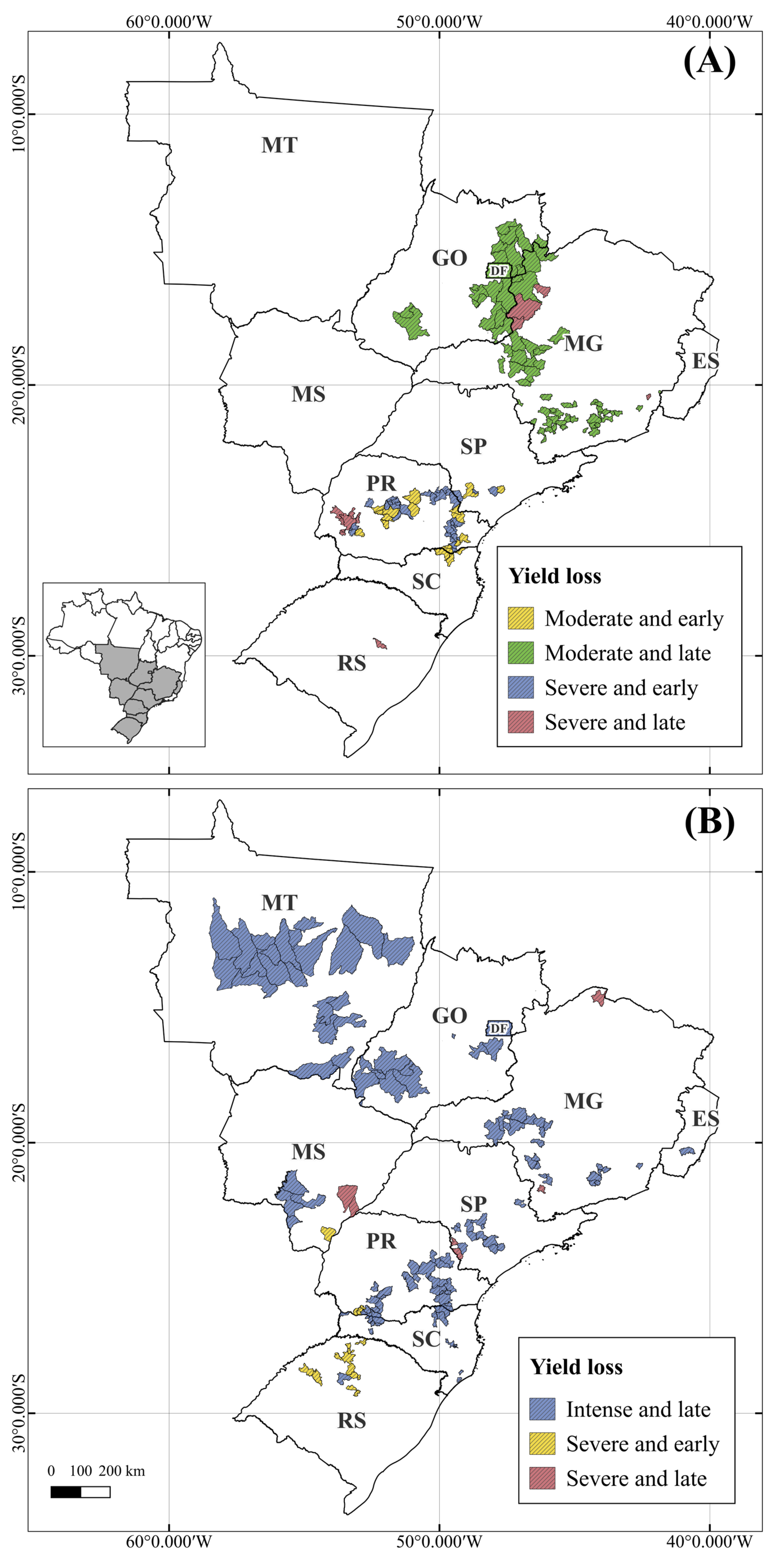
During the wet season, moderate and late yield loss predominates between latitudes −14.1° and −22.1° (Figure 2A, green color), encompassing municipalities in Goiás, Minas Gerais, and the Federal District, where the common bean sowing window extends from mid-October to late December. These areas are predominantly covered by the Cerrado biome and share similar soil and climatic characteristics, including low natural soil fertility and a tropical seasonal climate [49]. Pereira et al. [50] grouped these areas into the same macro-region for common bean cultivar recommendations in Brazil. Supporting these findings, Meireles et al. [51] observed a reduction in simulated attainable yield for common beans in Santo Antônio de Goiás (GO), from 1814 kg ha−1 for sowing on 20 October to 1685 kg ha−1 when sowing was delayed to 31 December. They further reported that the lowest yield-loss risks (<20%) occurred when sowing took place within the first 10 to 20 days of November. Heinemann et al. [15] found that optimal environments for wet-season common bean production in Goiás were characterized by higher annual rainfall, a narrower annual temperature range, and sowing between 1 and 20 November. Justino et al. [14,31] also observed reductions in simulated bean yields with delayed sowing in municipalities in Goiás, further corroborating our results.
In contrast, at latitudes between −23.8° and −29.6°, severe and early yield loss is more prevalent (Figure 2A, blue color), followed by moderate and early yield loss (Figure 2A, yellow color). These latitudes correspond to municipalities in Paraná, Rio Grande do Sul, Santa Catarina, and São Paulo, where common beans are sown between August and December. Table S3 (Supplementary Information) provides detailed yield-loss classification for each municipality and sowing date during the wet season.

3.1.1. Characterization of Municipalities with Sowing Between October and December

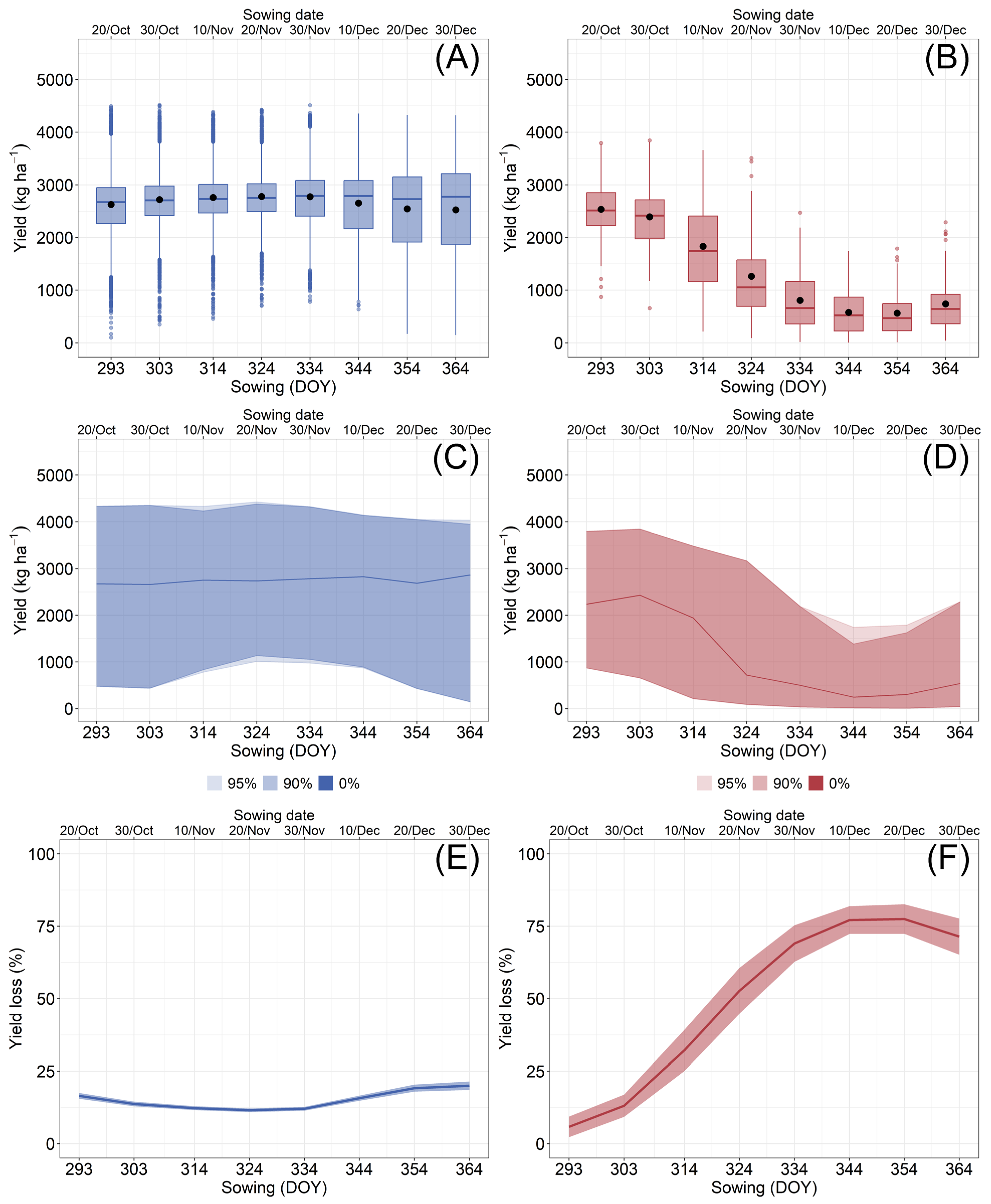
Simulated common bean yields (kg ha−1) for municipalities sown between October and December, classified as having either moderate and late yield loss (Figure 3A,C) or severe and late yield loss (Figure 3B,D), revealed contrasting patterns. In municipalities with moderate and late yield loss, average yields increased slightly as sowing was delayed from 20 October (2536 kg ha−1) to 20 November (2779 kg ha−1), followed by a decline at the final sowing date (2526 kg ha−1 on 30 December). Yield variability also increased with later sowing, with the standard deviation rising from 637 kg ha−1 (20 November) to 922 kg ha−1 (30 December). In contrast, municipalities experiencing severe and late yield loss showed a marked decline in yield as sowing was postponed, decreasing from 2536 kg ha−1 on 20 October to only 563 kg ha−1 on 20 December (Figure 3B,D). Overall, mean yields were substantially higher in the moderate and late yield loss group (2674 kg ha−1) than in the severe and late yield loss group (1338 kg ha−1).
For municipalities characterized by moderate and late yield loss, the lowest yield-loss rates (12–21.5%) were observed at earlier sowing dates, with losses increasing progressively toward 30 December (Figure 3E). Air temperature (mean maximum of 28 °C and minimum of 18 °C) and accumulated global solar radiation (average of 1686 MJ m−2) during the crop cycle varied little across sowing dates (Figure S4A,B, Supplementary Information). However, accumulated rainfall decreased from 728 mm (on 10 November) to 634 mm (on 30 December) (Figure S4C), while mean evapotranspiration remained stable at 369 mm per cycle (Figure S4D).
In municipalities with severe and late yield loss, yield-loss rates increased sharply between 20 October and 20 December, peaking at 83% (Figure 3F). Air temperatures in these areas remained relatively stable across sowing dates, with maximum temperatures averaging 29 °C and minimum temperatures averaging 19 °C (Figure S4A), which were higher than those recorded in the moderate and late yield-loss group. Solar radiation decreased from 20 October (1710 MJ m−2) to 20 November (1670 MJ m−2) and then increased to 1744 MJ m−2 on 30 December (Figure S4B). Accumulated rainfall peaked on 10 November (695 mm) and declined to 539 mm by the final sowing date (Figure S4C).
Comparing the yields between the two yield-loss groups (moderate and late, Figure 3A,C, and severe and late, Figure 3B,D) highlights the contrasting dynamics. In the severe and late group, yields declined sharply starting on 30 October (Figure 3B), while yield-loss rates increased more linearly and stabilized after 10 December (Figure 3F). Maximum and minimum temperatures were about 2 °C higher in municipalities affected by severe and late yield loss (Figure S4A) across all sowing dates. For this group, solar radiation remained lower until 30 November, increasing sharply thereafter for later sowing dates (Figure S4B). Differences in accumulated rainfall between the groups (moderate and late and severe and late) widened as sowing was delayed (Figure S4C), whereas total evapotranspiration was higher in the moderate and late yield-loss group, regardless of sowing date (Figure S4D).

3.1.2. Characterization of Municipalities with Sowing Between Mid-August and Late December

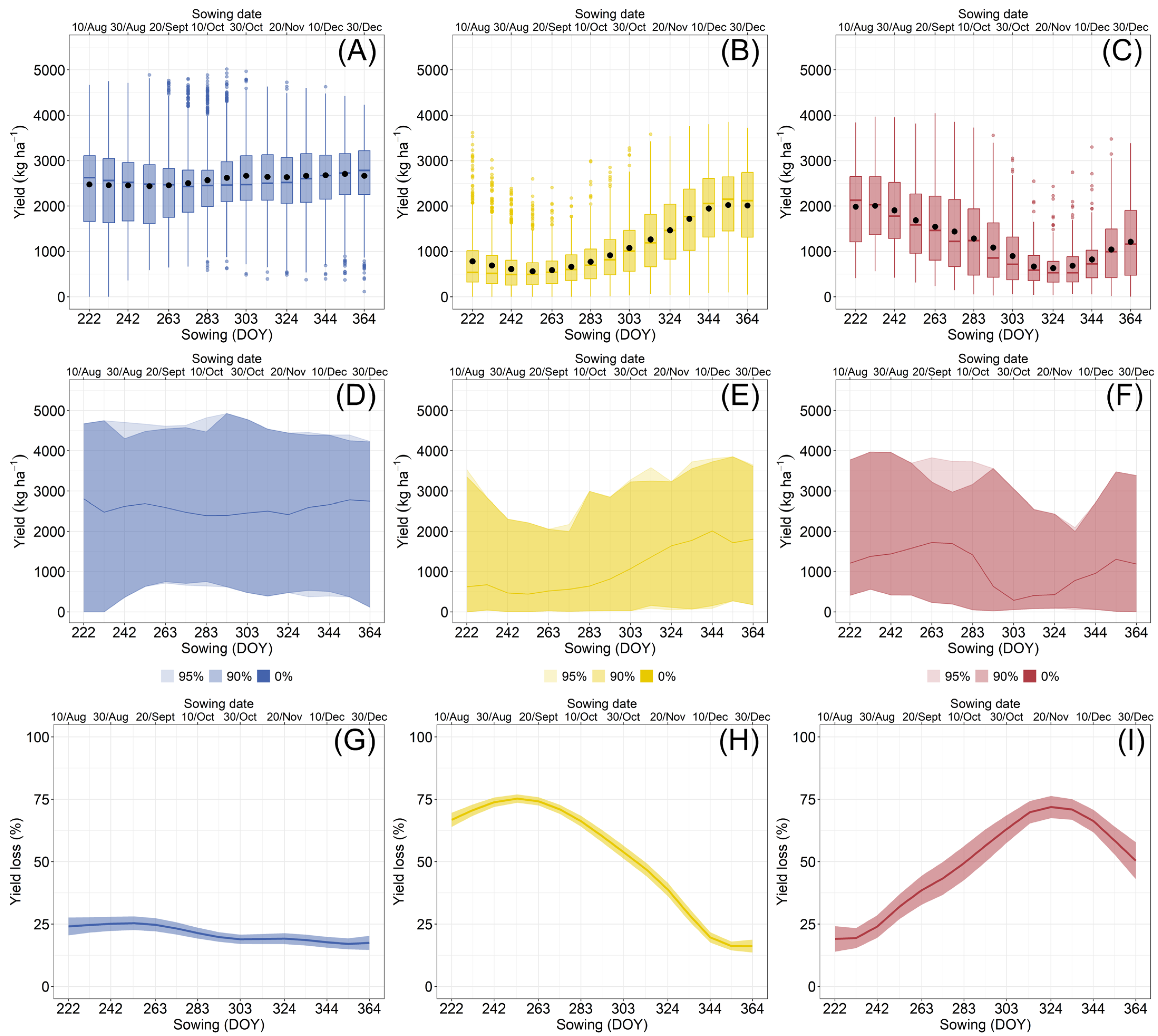
In municipalities with sowing between mid-August and late December classified as having moderate and early yield loss, mean yields decreased slightly from 10 August (2476 kg ha−1) to 10 September (2438 kg ha−1), followed by a steady increase until 20 December (2708 kg ha−1) (Figure 4A,D). For municipalities classified as severe and early yield loss (Figure 4B,E), yields increased as sowing was delayed. The lowest mean yield was recorded on 10 September (563 kg ha−1) and the highest on 20 December (2022 kg ha−1). Conversely, in municipalities classified as having severe and late yield loss, yields declined as sowing was delayed from 10 August (1986 kg ha−1) to 20 November (633 kg ha−1), followed by a partial recovery between 30 November (685 kg ha−1) and 30 December (1213 kg ha−1) (Figure 4C,F). Mean yields for these groups were 2577 kg ha−1 (moderate and early), 1139 kg ha−1 (severe and early), and 1260 kg ha−1 (severe and late).
The moderate and early yield-loss group showed the smallest reduction in maximum yield (28% on 10 September) (Figure 4G). This group also had the lowest average air temperatures across sowing dates, which increased as sowing was delayed (Figure S5A, Supplementary Information). Maximum temperatures ranged from 24.6 °C on 10 August to 27.6 °C on 30 December, while minimum temperatures increased from 13.5 °C to 17.5 °C over the same period. For optimal yields, common bean requires minimum, optimum, and maximum air temperature of 12 °C, 21 °C, and 29 °C, respectively [52]. Air temperatures below 12 °C during the vegetative phase (from emergence to the formation of the third fully developed trifoliate leaf, V0–V4 [53]) slow plant growth, and when such temperatures occur near flowering, they may induce flower abortion, reducing bean yields [54].
In municipalities with severe and early yield-loss group, yield losses decreased as sowing was delayed, from 77% (10 September) to 18% (20 December) (Figure 4H). In contrast, for the severe and late yield-loss group the highest loss (76%) occurred on 20 November and the lowest loss (24%) on 10 August (Figure 4I). As observed in the moderate and early yield-loss group, air temperatures increased with later sowing dates (Figure S5A). In the severe and early yield-loss group, temperatures ranged from 19.7 °C (10 August) to 23 °C (30 December), whereas in the severe and late yield-loss group, they ranged from 21.2 °C to 25 °C across sowing dates. In this region, encompassing São Paulo and southern Brazil, air temperature is a key limiting factor for common bean yield. Caramori et al. [55] reported that in the western and northwestern regions of Paraná, where the municipalities classified as severe and late yield loss are located, air temperatures often exceed the ideal range (12 °C to 29 °C) for common bean cultivation. Additionally, the risk of water deficit during flowering increases from November onward, further reducing yields. In contrast, in the southern and southeastern regions of Paraná, where some of the municipalities classified in the severe and early loss group are located, these risks are lower for later sowing dates. However, sowing between August to September increases the crop’s susceptibility to frost, substantially elevating yield-loss risk [56].
All yield-loss groups showed similar patterns of accumulated global solar radiation across sowing dates (Figure S5B). In the moderate and early yield-loss group, solar radiation peaked on 30 September (1919 MJ m−2) and reached its lowest value on 30 December (1693 MJ m−2). A similar trend was observed for the severe and early group, with maximum solar radiation on 30 September (1951 MJ m−2) and minimum on 30 December (1696 MJ m−2). In the severe and late yield-loss group, solar radiation peaked on 20 October (1946 MJ m−2) and declined to its lowest value on 30 December (1760 MJ m−2).
During earlier sowing dates (10 August–20 October), the severe and early yield-loss group experienced the lowest accumulated rainfall and evapotranspiration, contributing to reduced yields in this period. Conversely, during later sowing dates (30 October to 30 December), which correspond to the lowest yields in the severe and late yield-loss group, accumulated rainfall was lower for this group compared with the others (Figure S5C).

3.2. Dry-Season Common Bean Yield Loss

The dry season is predominantly characterized by the intense and late yield-loss group (83%) (Figure 2B, blue color). In municipalities where common beans are sown between January and early March (in the states of Goiás, Mato Grosso, Mato Grosso do Sul, the Federal District, Minas Gerais, São Paulo, and Rio Grande do Sul), the intense and late yield-loss group is prevalent between latitudes −11.9 and −22.9 (Figure 2B, blue color). At lower latitudes (between −23.5 and −29.33), a higher occurrence of severe and early yield-loss group is observed (Figure 2B, yellow color). Similarly, in municipalities where sowing occurs between January and late March (in the states of Espírito Santo, Paraná, Santa Catarina, and São Paulo), most municipalities (91%) were classified as experiencing intense and late yield loss. Detailed yield-loss classification for each municipality and sowing date during the dry season is presented in Table S4 (Supplementary Information).

3.2.1. Characterization of Municipalities with Sowing Between January and Early March

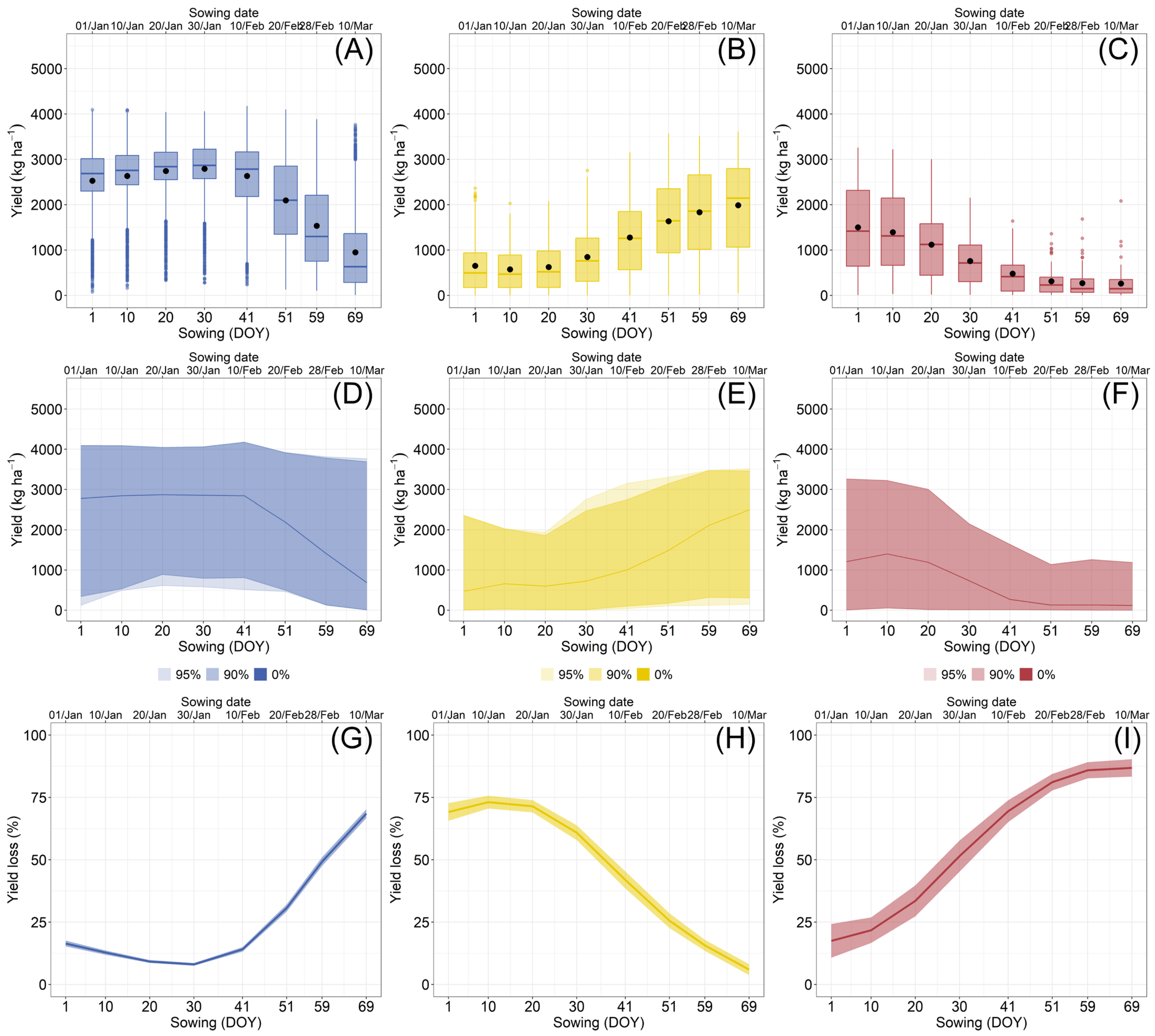
Municipalities with dry-season sowing between January and early March were classified into three groups: intense and late yield loss (Figure 5A,D), severe and early yield loss (Figure 5B,E), and severe and late yield loss (Figure 5C,F). In the late-loss groups (intense and late; severe and late), average yields decreased as sowing was delayed. In contrast, in the severe and early yield loss, yields increased with later sowing dates (Figure 5B,E). For the intense and late group, maximum and minimum yields were 2790 kg ha−1 (30 January) and 949 kg ha−1 (10 March), respectively. In the severe and early group, yields ranged from 573 kg ha−1 (10 January) to 1988 kg ha−1 (10 March). For the severe and late group, the highest yield (1500 kg ha−1) occurred on 1 January, while the lowest (262 kg ha−1) was recorded on 10 March.
Figure 5G–I illustrate the mean functional yield-loss curves (%) as a function of dry-season sowing dates. The sowing dates associated with the highest yields coincided with the lowest yield losses and were, therefore, the most suitable periods for planting. Conversely, dates with the lowest yields corresponded to the greatest losses, indicating less favorable growing conditions. Maximum yield losses reached 70% (10 March) in municipalities classified as intense and late yield loss, 76% (10 January) for municipalities with severe and early yield loss, and 90% (10 March) for municipalities with severe and late yield loss.
The late-loss groups (intense and late; severe and late), predominantly located in the Midwest region and in Minas Gerais, exhibited little variation in maximum and minimum temperatures across sowing dates (Figure S6A). In the intense and late group, maximum air temperature ranged from 29.7 °C (1 January) to 28.8 °C (10 March), while minimum temperatures decline from 19.5 °C to 17.4 °C (over the same period). In the severe and late group, maximum air temperatures ranged from 30.9 °C (1 January) to 28.6 °C (10 March) and minimum temperatures from 20.2 °C (1 January) to 17.1 °C (10 March).
In contrast, the severe and early yield-loss group showed greater variation in both air temperature and accumulated global solar radiation across sowing dates. Maximum temperature decreased from 29.8 °C (1 January) to 24.7 °C (10 March), while minimum temperatures declined from 19 °C (1 January) to 14.5 °C (10 March). Solar radiation also declined, from 1740 MJ m−2 per cycle to 1536 MJ m−2 per cycle between the first and last sowing dates (Figure S6B).
Rainfall was inversely related to yield loss, with higher yield losses observed at sowing dates with lower rainfall (Figure S6C). In the late-loss groups, rainfall decreased as sowing was delayed, with values ranging from 688 mm (1 January) to 284 mm (10 March) for the intense and late-loss group and from 463 mm to 246 mm for the severe and late-loss group. For the severe and early loss group, rainfall ranged from 407 mm to 536 mm between these dates.
The increase in yield losses was exacerbated by low rainfall during the crop’s reproductive phase (from pre-flowering to the maturation phase (R5–R9) [53]), particularly in municipalities classified as experiencing severe and late yield loss. Water deficits occur when evapotranspiration exceeds root water uptake, a condition that is especially detrimental to grain yield [57]. The impact of water stress depends on its timing, duration, and intensity [58]. Common bean is particularly sensitive to drought during flowering and grain filling [53]. Water deficits during flowering can induce flower abortion, while stress during grain filling may lead to abortion of fertilized ovules within pods, ultimately reducing yield [6]. For later sowing dates during the dry season, municipalities classified as experiencing late yield loss often faced rainfall levels during the reproductive phase below crop requirements, thereby increasing yield losses [53].
Common bean requires between 200 and 350 mm of water, ideally well distributed throughout the crop cycle [53,59]. Although total rainfall during most dry-season sowing periods falls within this range, uniform distribution is critical [60]. Reduced and poorly distributed rainfall at later sowing dates increases the likelihood of water deficits during the reproductive phase. Conversely, higher and better-distributed rainfall during both the vegetative and reproductive phases on earlier sowing dates contributed to a lower yield-loss risk for common beans. Therefore, careful planning of sowing dates based on regional rainfall patterns is essential to mitigate the negative effects of water stress on yield [61]. Adequate water supply at critical growth stages is essential for sustaining leaf expansion, photosynthesis, and dry matter accumulation.

3.2.2. Environmental Characterization of Municipalities with Sowing Between January and Late March

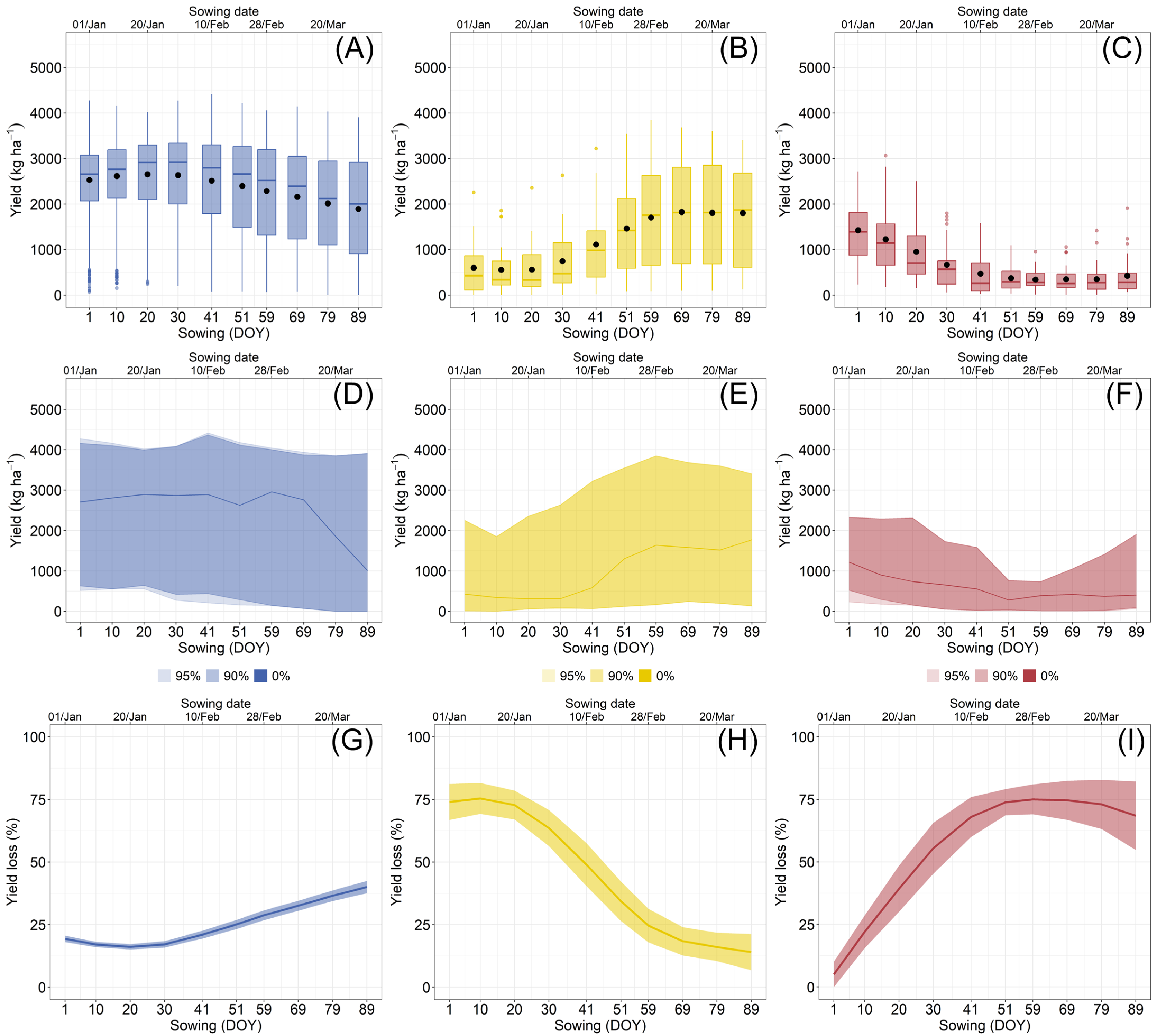
Figure 6 illustrates the simulated yields (kg ha−1) for municipalities sowing common bean during the dry season between January and late March. In the intense and late-loss group (Figure 6A,D), which had an average yield of 2370 kg ha−1, yield decreased as sowing was delayed. The highest yield (2652 kg ha−1) occurred on 20 January and the lowest (1892 kg ha−1) on 30 March, coinciding with group’s maximum yield loss (42%) (Figure 6G).
A similar pattern was observed in the severe and late-loss group (Figure 6C,F), where significant yield reductions occurred when sowing was delayed beyond mid-January. Yield loss exceeded 40% after this period, peaking at 83% for sowing on 20 March (Figure 6I). In contrast, the severe and early loss group (Figure 6B,E) showed increasing yields as sowing was delayed, with maximum values achieved from 10 March onward. The lowest yield loss (21%) was recorded on the last sowing date (30 March), whereas the highest (81%) occurred on the earliest sowing dates (1 and 10 January) (Figure 6H).
Across all groups, later sowing dates were associated with lower air temperature and reduced accumulated solar radiation (Figure S7A,B, Supplementary Information). Maximum air temperatures ranged from 28.3 °C (1 January) to 23 °C (30 March), while minimum temperatures decreased from 18.1 °C (1 January) to 12.7 °C (30 March) over the same period. On average, both maximum and minimum air temperatures in the severe and late-loss group were 0.88 °C higher than in the other groups. In contrast, accumulated solar radiation in the severe and early loss group was approximately 111 MJ m−2 greater.
Global solar radiation is a crucial factor in agricultural production. Crop yield depends on the amount of incident solar radiation, the crop’s ability to intercept it, and its radiation use efficiency [62,63,64]. During the dry season, later sowing dates are associated with lower yields due to reduced accumulated global solar radiation. This reduction limits photosynthetic activity, particularly during critical growth stages such as flowering and grain filling, ultimately decreasing biomass accumulation and grain production [65].
The severe and early yield-loss group also recorded the highest average rainfall (596 mm), with totals ranging from 477 mm (10 January) to 644 mm (30 March). In the intense and late-loss group, rainfall varied only slightly among sowing dates, from 402 mm (20 February) to 488 mm (1 January). In contrast, the severe and late-loss group exhibited a marked decline in rainfall, from 494 mm (1 January) to 303 mm (20 March) (Figure S7C).

3.3. Environmental Covariates

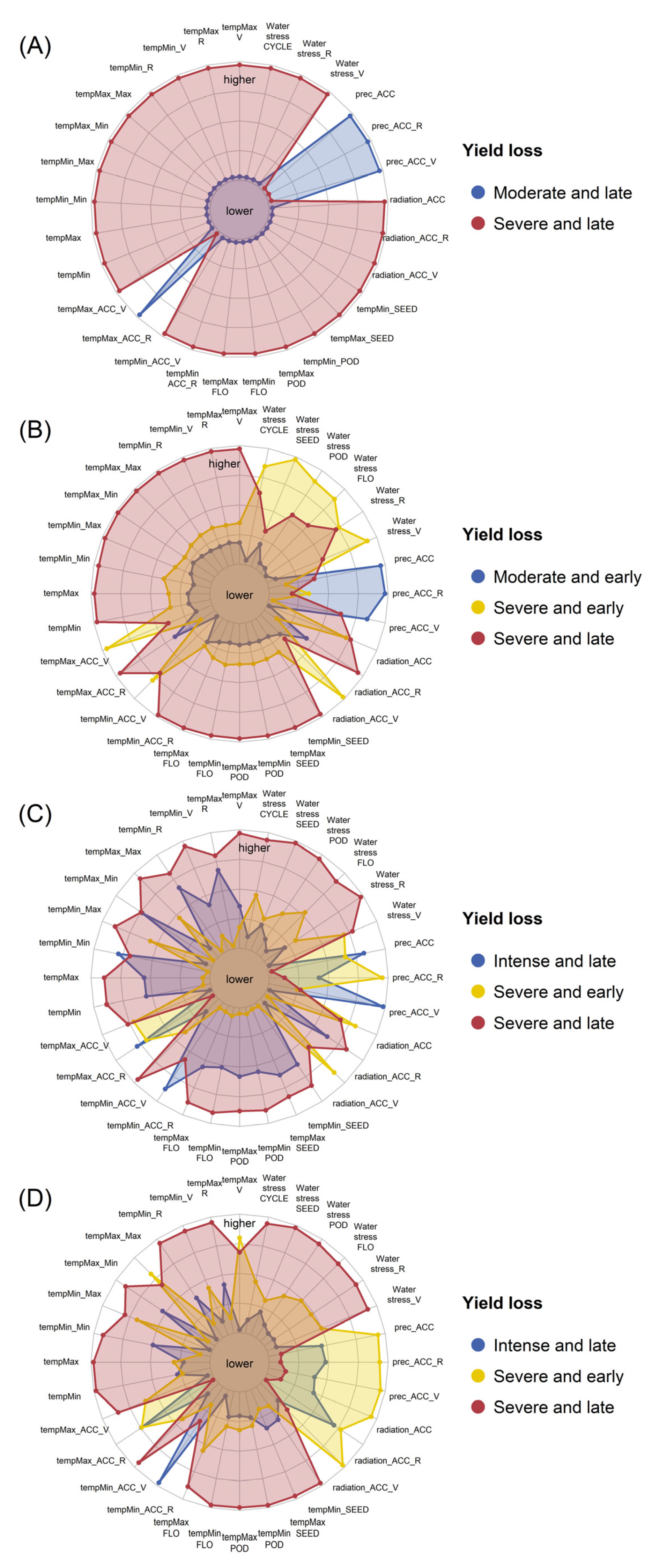
Figure 7A,B presents radar graphs illustrating the characterization of environmental covariates during the common bean growing cycle for yield-loss groups of municipalities with sowing in the wet season between October and December (A) and between August and December (B). For municipalities sowing between October and December (Figure 7A), the moderate and late yield-loss group, located in the states of Goiás, Minas Gerais, and the Federal District, exhibited higher values for all rainfall-related covariates and for the maximum accumulated air temperature during the reproductive stage (tempMax_ACC_R). In contrast, the severe and late yield-loss group, composed of municipalities in Minas Gerais, showed the highest values for all water stress covariates, solar radiation, and air temperature covariates, except for tempMax_ACC_R (Figure 7A).
For municipalities sowing in the wet season between August and December, located in the southern states of Brazil and São Paulo (Figure 7B), the moderate and early yield-loss group displayed higher values for all rainfall covariates. On the other hand, the severe and early yield-loss group showed higher values for all water stress covariates, as well as for tempMax_ACC_V and tempMin_ACC_V. Except for these two temperature covariates, the severe and late yield-loss group exhibited higher values for all other covariates.
Figure 7C,D shows radar graphs of environmental covariates during the common bean cycle for municipalities sowing in the dry season between January and early March (C) and between January and late March (D). For municipalities sowing between January to early March, the severe and late yield-loss group, comprising municipalities in the Southeast and Midwest regions, exhibited the highest values for all water stress covariates, accumulated solar radiation during the reproductive stage (radiation_ACC_R), and most air temperature covariates. Heinemann et al. [59] reported that climatic factors influence common bean yield differently across Brazilian regions and growing seasons. During the dry season, the Midwest region experienced higher air temperature values, lower accumulated rainfall, and lower global solar radiation compared to the South. In contrast, the highest values for tempMin_Min, tempMax_ACC_R, tempMin_ACC_R, prec_ACC, and prec_ACC_V occurred in the group with intense and late yield loss. Meanwhile, the severe and early yield-loss group showed higher values for prec_ACC_R, radiation_ACC, and radiation_ACC_V (Figure 7C).
Similarly, for municipalities sowing between January and late March (Figure 7D), the severe and late yield-loss group displayed higher values for all water stress covariates and most air temperature covariates. In contrast, the severe and early yield-loss group exhibited the highest values for rainfall and global solar radiation.

3.4. Common Bean Sowing Calendar

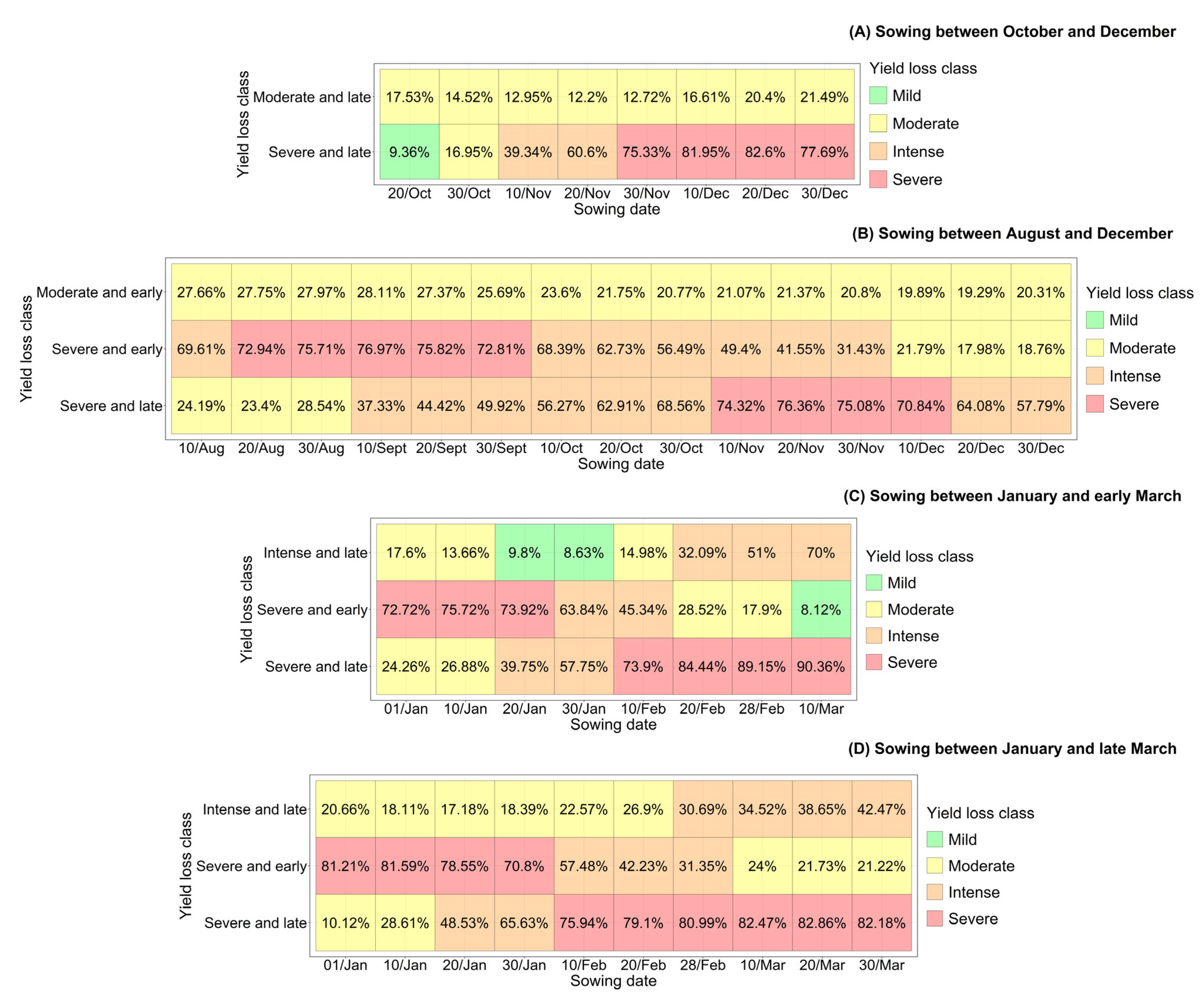
Figure 8A,B shows the common bean sowing calendars for each group of municipalities during the wet season. For municipalities sowing between October and December (Figure 8A), the optimal sowing period, characterized by the lowest yield loss, was between 10 November and 30 November for the moderate and late yield-loss group and between 20 October and 30 October for the severe and late yield-loss group. For the latter group, sowing within this window resulted in mild and moderate yield losses, while later sowing led to severe losses (>70%).
For municipalities sowing between August and December in the wet season (Figure 8B), the periods associated with the lowest yield loss were between 10 December and 20 December for the moderate and early loss group, between 20 December and 30 December for the severe and early loss group, and between 10 August and 20 August for the group classified as severe and late loss.
Overall, the ideal sowing period for common beans during the wet season depends on the timing of minimum and maximum yield loss. In municipalities classified with early yield loss, sowing should be carried out in mid-December. However, in municipalities located in Goiás, Minas Gerais, and the Federal District, classified with late yield loss, sowing should occur in October. In municipalities in Paraná, also classified as late yield loss, August sowing results in the lowest yield loss. This variation underscores regional disparities, which are further evidenced by the sowing calendar, which demonstrated clear spatial heterogeneity. Earlier sowing windows predominate in southern and southeastern Brazil, while progressively later sowing dates are observed toward lower latitudes. This pattern aligns with latitudinal differences in photoperiod and temperature, as well as variations in the onset of the rainy season.
Figure 8C,D presents the sowing calendars for the dry season. For municipalities classified with intense and late yield loss, the most favorable sowing period was mid-January, regardless of the sowing window considered. In municipalities classified with severe and early yield loss, the most suitable sowing dates occurred in March. For those in severe and late yield-loss group, the optimal sowing window was between 1 January and 10 January.
Given the robust nature of the calendar derived from historical data, it is imperative to consider how future climate change might alter its utility and accuracy. Brazil’s climate is projected to undergo significant transformations, particularly regarding rainfall variability and increased temperatures. By the end of this century, the global average temperature is projected to rise by approximately 3.2 °C due to increasing greenhouse gas emissions. Drought events are expected to become more frequent and intense as climate change progresses [66]. Furthermore, research suggests that the frequency and intensity of El Niño-Southern Oscillation (ENSO) events may increase as a result of climate change, leading to more severe droughts in some regions and floods in others [67,68,69,70].
Although climate change will have detrimental effects on agricultural production, the rise in air temperature could benefit cold-climate regions, such as southern Brazil, by creating new opportunities for growing beans in different seasons. However, this temperature increase also impacts other environmental factors, including water availability, wind patterns, and the intensity and duration of sunlight [71]. These effects are expected to be particularly detrimental to sensitive crops like beans, especially in regions with hot and dry climates and suboptimal soil properties, such as the Brazilian Cerrado.
Rattis et al. [72] reported that, despite agricultural expansion and intensification, episodes of hot and dry weather during drought events have led to a reduction in crop yields along the Amazon-Cerrado agricultural frontier. Similarly, Hofmann et al. [73] showed that the suppression of native vegetation and forest fires experienced over the past three decades in the Brazilian Cerrado region have resulted in spatial changes at local and regional scales. The authors emphasize that, in this region, average temperatures have increased, and relative humidity has decreased between 1961 and 2019.
Higher temperatures can accelerate phenological development, shorten the grain-filling period, and intensify reproductive stress. In this perspective, strategies such as supplemental irrigation, the development of drought-tolerant cultivars, preservation of native vegetation, and soil management practices aimed at improving physicochemical properties may help mitigate the negative impacts of climate change on agricultural crops [72,74]. Furthermore, the climatic shifts may require dynamic updating of the sowing calendar based on seasonal forecasts and decadal projections.
Despite the valuable insights provided, the DSSAT CSM-CROPGRO-Dry Bean model presents inherent limitations. It operates on daily weather data, potentially missing crucial sub-daily extremes (e.g., heatwaves) and utilizes generalized soil and management profiles that may not represent local heterogeneity in practices or conditions. Furthermore, genetic coefficients typically reflect a representative cultivar, failing to capture genotypic variability across regions. The model does not account for crop disease, socioeconomic factors such as labor availability, market access, or mechanization, which also influence planting decisions. Moreover, the sowing calendar derived from this model is based on historical climate data, which may not hold under future climate regimes. Without dynamic integration of climate projections, these recommendations risk becoming outdated as climatic conditions evolve [75].
However, the spatio-temporal sowing calendar developed in this study provides valuable information for pricing yield-loss risks in common bean crops associated with climatic factors. It highlights sowing dates with the highest or lowest yield-loss risk, depending on the season. Risk pricing is a key factor in insurance contracts. Accurate risk pricing requires reliable statistical data and appropriate methodologies for each segment [76]. Rural producers often rely on cost-based or yield insurance to mitigate the risks associated with adverse weather conditions.

4. Conclusions

This study demonstrates that the strategic adjustment of sowing dates constitutes a pivotal, yet highly region-specific, lever for enhancing the climate resilience of rainfed common bean production in Central-Southern Brazil. By integrating the CSM-CROPGRO-Dry Bean model with Functional Data Analysis (FDA), we moved beyond discrete sowing-date comparisons to model the continuous yield-loss risk profile across the entire sowing window. This novel methodological approach enabled the synthesis of complex spatio-temporal patterns into actionable insights.
Our results define a clear, spatially differentiated sowing calendar. For the main (wet) season, the optimal strategy diverges geographically: earlier sowing minimizes climatic risk in the core Midwest and Central Highlands (Goiás, Minas Gerais, Federal District, and western Paraná), whereas later sowing is more advantageous in southern and southeastern regions (São Paulo, Santa Catarina, and eastern Paraná). In the dry season, earlier sowing consistently represents the lower-risk strategy across the vast majority of municipalities. These patterns are mechanistically explained by the degree of alignment between critical reproductive stages and periods of water deficit or suboptimal temperatures, with solar radiation exerting a secondary, though still relevant, influence.
These findings provide an evidence-based decision-support tool directly applicable to farm management, allowing producers to tailor sowing dates according to their local climatic risk profile. Crucially, the functional risk curves and resulting spatial clusters also offer a robust quantitative foundation for policymakers and financial institutions. Such information is essential for designing targeted agricultural extension programs, optimizing regional adaptation strategies, and developing actuarially sound and equitable crop insurance schemes that accurately reflect localized production risks.
In the context of sustainable intensification, this study underscores that adapting to climate variability need not rely solely on high-input technological solutions. Optimizing low-cost agronomic practices, informed by sophisticated spatio-temporal analysis, represents a fundamental pathway toward stabilizing yields, safeguarding livelihoods, and strengthening the resilience of a vital food system. Future research can build upon this FDA framework to incorporate climate change projections, evaluate additional cultivars, and integrate other adaptive management practices, thereby further refining strategies for sustainable bean production under increasing climatic uncertainty.

Supplementary Materials

The following supporting information can be downloaded at https://www.mdpi.com/article/10.3390/resources15030040/s1, Figure S1: Description of the process for obtaining yield-loss curves for the municipality of Rio Verde during the wet season: (A) simulated yield curves (kg ha−1) per year (from 1980 to 2016), considering the set of sowing dates from day of year (DOY) 293 to 364; and (B) yield-loss curves (%) per year (from 1980 to 2016), considering the set of sowing dates from day of year (DOY) 293 to 364; Figure S2: Description of the clustering process of yield-loss curves using functional data analysis techniques: (A) clustering of yield-loss curves into three groups, considering the set of sowing dates from day of year (DOY) 1 to 69 during the dry season; and (B) average yield-loss curve for each group of municipalities; Figure S3: Description of the clustering process of yield-loss curves with the same sequence of sowing dates during the wet season. The gray lines represent the yield-loss curves for each municipality/year, while the black line illustrates the average yield-loss curve adjusted by functional data analysis (FDA) for the entire group of municipalities, considering the set of sowing dates from day of year (DOY) 293 to 364.; Figure S4: Median values for maximum and minimum air temperature (°C) (A), accumulated global solar radiation (MJ m−2 cycle−1) (B), accumulated rainfall (mm cycle−1) (C), and evapotranspiration (mm cycle−1) (D) for the groups of municipalities with sowing between mid-October and late December in the wet season, with moderate and late (blue) and severe and late (red) yield loss, depending on the sowing date; Figure S5: Median values for maximum and minimum air temperature (°C) (A), accumulated global solar radiation (MJ m−2 cycle−1) (B), accumulated rainfall (mm cycle−1) (C), and evapotranspiration (mm cycle−1) (D) for the groups of municipalities with sowing between mid-August and late December in the wet season, with moderate and early (blue), severe and early (yellow), and severe and late (red) yield loss, depending on the sowing date. Figure S6: Median values for maximum and minimum air temperature (°C) (A), accumulated global solar radiation (MJ m−2 cycle−1) (B), accumulated rainfall (mm cycle−1) (C), and evapotranspiration (mm cycle−1) (D) for the groups of municipalities with sowing between January and early March in the dry season, with intense and late (blue), severe and early (yellow), and severe and late (red) yield loss, depending on the sowing date; Figure S7: Median values for maximum and minimum air temperature (°C) (A), accumulated global solar radiation (MJ m−2 cycle−1) (B), accumulated rainfall (mm cycle−1) (C), and evapotranspiration (mm cycle−1) (D) for the groups of municipalities with sowing between January and late March in the dry season, with intense and late (blue), severe and early (yellow), and severe and late (red) yield loss, depending on the sowing date. Table S1: Selected common bean-producing municipalities during the wet season, including their respective states, predominant soil classes, and sowing periods (initial and final dates) based on the Agricultural Zoning for Climate Risk (ZARC); Table S2: Selected common bean-producing municipalities during the dry season, including their respective states, predominant soil classes, and sowing periods (initial and final dates) based on the Agricultural Zoning for Climate Risk (ZARC); Table S3: Common bean-producing municipalities during the wet season selected for this study, their respective yield-loss classes and sowing periods; Table S4: Common bean-producing municipalities during the dry season selected for this study, their respective yield-loss classes and sowing periods; Table S5: Specific genetic coefficients for CMS-CROPGRO-Drybean obtained by the parameterization process for the common bean cultivar BRS Estilo; Table S6: Soil parameters used in the simulations were obtained from the HYBRAS database [1], except for those corresponding to Ferralsol soils. For Ferralsol, parameters were sourced from the Embrapa Rice & Beans database, compiled by the Common Bean Breeding Program for each multi-environment trial (MET); Table S7: Acronyms for the environmental features (EF) applied in this study.

Author Contributions

Conceptualization, L.F.J. and D.H.d.M.; Methodology, L.F.J., F.W.A. and D.H.d.M.; Investigation, L.F.J., A.B.H., F.W.A. and D.H.d.M.; Data Curation, A.B.H.; Software, F.W.A.; Visualization, F.W.A. and L.F.J.; Writing—Original Draft, L.F.J. and D.H.d.M.; Writing—Review and Editing, L.F.J., A.B.H., D.H.d.M., L.F.S. and S.C.d.S.; Funding Acquisition, A.B.H.; Supervision, A.B.H. and D.H.d.M. All authors have read and agreed to the published version of the manuscript.

Funding

The authors declare that they have no known competing financial interests or personal relationships that could have appeared to influence the work reported in this paper.

Data Availability Statement

Data will be made available on request.

Conflicts of Interest

The authors declare no competing interests.

References

  1. Şimşek, O. Harvesting sustainability: Innovations and practices in modern agriculture. Green Technol. Sustain. 2025, 3, 100192. [Google Scholar] [CrossRef] [Scilit]
  2. Verma, K.K.; Song, X.-P.; Kumari, A.; Jagadesh, M.; Singh, S.K.; Bhatt, R.; Singh, M.; Seth, C.S.; Li, Y.-R. Climate change adaptation: Challenges for agricultural sustainability. Plant Cell Environ. 2025, 48, 2522–2533. [Google Scholar] [CrossRef] [Scilit] [PubMed]
  3. CGIAR. Consultative Group on International Agricultural Research. Importance of Bean Crop Research. 2025. Available online: https://alliancebioversityciat.org/crops/beans/importance (accessed on 28 July 2025).
  4. Broughton, W.J.; Hernández, G.; Lair, M.; Beebe, S.; Gepts, P.; Venderleyden, J. Beans (Phaseolus spp.)—Model food legumes. Plant Soil 2003, 252, 55–128. [Google Scholar] [CrossRef] [Scilit]
  5. Heinemann, A.B.; Ramirez-Villegas, J.; Stone, L.F.; Didonet, A.D. Climate change determined drought stress profiles in rainfed common bean production systems in Brazil. Agric. For. Meteorol. 2017, 246, 64–77. [Google Scholar] [CrossRef] [Scilit]
  6. Mathobo, R.; Marais, D.; Steyn, J.M. The effect of drought stress on yield, leaf gaseous exchange and chlorophyll fluorescence of dry beans (Phaseolus vulgaris L.). Agric. Water Manag. 2017, 180, 118–125. [Google Scholar] [CrossRef] [Scilit]
  7. Kazai, P.; Noulas, C.; Khah, E.; Vlachostergios, D. Yield and seed quality parameters of common bean cultivars grown under water and heat stress field conditions. AIMS Agric. Food 2019, 4, 285–302. [Google Scholar] [CrossRef] [Scilit]
  8. Rai, A.; Sharma, V.; Heitholt, J. Dry bean [Phaseolus vulgaris L.] growth and yield response to variable irrigation in the arid to semi-arid climate. Sustainability 2020, 12, 3851. [Google Scholar] [CrossRef] [Scilit]
  9. Vargas, Y.; Mayor-Duran, V.M.; Buendia, H.F.; Ruiz-Guzman, H.; Raatz, B. Physiological and genetic characterization of heat stress effects in a common bean RIL population. PLoS ONE 2021, 16, e0249859. [Google Scholar] [CrossRef] [Scilit]
  10. Tene, T.M.; Sari, H.; Canci, H.; Maaruf, A.; Eker, T.; Toker, C. Traits related to heat stress in Phaseolus Species. Agriculture 2023, 13, 953. [Google Scholar] [CrossRef] [Scilit]
  11. Casadebaig, P.; Zheng, B.; Chapman, S.; Huth, N.; Faivre, R.; Chenu, K. Assessment of the potential impacts of wheat plant traits across environments by combining crop modeling and global sensitivity analysis. PLoS ONE 2016, 11, e0146385. [Google Scholar] [CrossRef] [Scilit]
  12. Ramirez-Villegas, J.; Milão, A.M.; Alexandrov, N.; Asseng, S.; Challinor, A.J.; Crossa, J.; Van Eeuwijk, F.; Ghanem, M.E.; Grenier, C.; Heinemann, A.B.; et al. CGIAR modeling approaches for resource-constrained scenarios: I. Accelerating crop breeding for a changing climate. Crop Sci. 2020, 60, 547–567. [Google Scholar] [CrossRef] [Scilit]
  13. Khan, S.; Anwar, S.; Ashraf, M.Y.; Khaliq, B.; Sun, M.; Hussain, S.; Gao, Z.; Noor, H.; Alam, S. Mechanisms and adaptation strategies to improve heat tolerance in rice: A review. Plants 2019, 8, 508. [Google Scholar] [CrossRef] [Scilit] [PubMed]
  14. Justino, L.F.; Alves Júnior, J.; Battisti, R.; Heinemann, A.B.; Leite, C.V.; Evangelista, A.W.P.; Casaroli, D. Assessment of economic returns by using a central pivot system to irrigate common beans during the rainfed season in Central Brazil. Agric. Water Manag. 2019, 224, 105749. [Google Scholar] [CrossRef] [Scilit]
  15. Heinemann, A.B.; Ramirez-Villegas, J.; Souza, T.L.P.O.; Didonet, A.D.; Di Stefano, J.G.; Boote, K.J.; Jarvis, A. Drought impact on rainfed common bean production areas in Brazil. Agric. For. Meteorol. 2016, 225, 57–74. [Google Scholar] [CrossRef] [Scilit]
  16. Alam, A.S.A.F.; Begum, H.; Masud, M.M.; Al-Amin, A.Q.; Leal Filho, W. Agriculture insurance for disaster risk reduction: A case study of Malaysia. Int. J. Disaster Risk Reduct. 2020, 47, 101626. [Google Scholar] [CrossRef] [Scilit]
  17. Budhathoki, N.K.; Lassa, J.A.; Pun, S.; Zander, K.K. Farmers’ interest and willingness-to-pay for index-based crop insurance in the lowlands of Nepal. Land Use Policy 2019, 85, 1–10. [Google Scholar] [CrossRef] [Scilit]
  18. Vyas, S.; Dalhaus, T.; Kropff, M.; Aggarwal, P.; Meuwissen, M.P.M. Mapping global research on agricultural insurance. Environ. Res. Lett. 2021, 16, 103003. [Google Scholar] [CrossRef] [Scilit]
  19. Madaki, M.Y.; Kaechele, H.; Bavorova, M. Agricultural insurance as a climate risk adaptation strategy indeveloping countries: A case of Nigeria. Clim. Policy 2023, 23, 747–762. [Google Scholar] [CrossRef] [Scilit]
  20. Jame, Y.W.; Cutforth, W. Crop growth models for decision support systems. Can. J. Plant Sci. 1996, 76, 9–19. [Google Scholar] [CrossRef] [Scilit]
  21. Jones, J.W.; Antle, J.M.; Basso, B.; Boote, K.J.; Conant, R.T.; Foster, I.; Godfray, H.C.J.; Herrero, M.; Howitt, R.E.; Janssen, S.; et al. Brief history of agricultural systems modeling. Agric. Syst. 2017, 155, 240–254. [Google Scholar] [CrossRef] [Scilit]
  22. Battisti, R.; Sentelhas, P.C. Characterizing Brazilian soybean-growing regions by water deficit patterns. Field Crops Res. 2019, 240, 95–105. [Google Scholar] [CrossRef] [Scilit]
  23. Justino, L.F.; Heinemann, A.B.; da Matta, D.H.; Stone, L.F.; de Oliveira Gonçalves, P.A.; da Silva, S.C. Characterization of common bean production regions in Brazil using machine learning techniques. Agric. Syst. 2025, 224, 104237. [Google Scholar] [CrossRef] [Scilit]
  24. Justino, L.F.; Heinemann, A.B.; da Matta, D.H.; Stone, L.F.; de Oliveira Gonçalves, P.A.; da Silva, S.C. Spatio-temporal dynamics of water stress for common bean production in Goiás, Brazil. Theor. Appl. Climatol. 2025, 156, 224. [Google Scholar] [CrossRef] [Scilit]
  25. Antolin, L.A.S.; Heinemann, A.B.; Marin, F.R. Impact assessment of common bean availability in Brazil under climate change scenarios. Agric. Syst. 2021, 191, 103174. [Google Scholar] [CrossRef] [Scilit]
  26. da Matta, D.H.; dos Santos Coelho, C.A.; dos Santos, L.L.; Stone, L.F.; Heinemann, A.B. Analysis of Goiás State rainfall and temperature similarity patterns during the El Niño-Southern Oscillation phenomenon phases across the years. Theor. Appl. Climatol. 2023, 153, 1013–1031. [Google Scholar] [CrossRef] [Scilit]
  27. IBGE (Instituto Brasileiro de Geografia e Estatística). Produção Agrícola Municipal. 2020. Available online: https://sidra.ibge.gov.br/pesquisa/pam/tabelas (accessed on 3 November 2021).
  28. Conab (Companhia Nacional de Abastecimento). Acompanhamento da Safra Brasileira Grãos—12° Levantamento—Safra 2024/25. 2025. Available online: https://www.gov.br/conab/pt-br/atuacao/informacoes-agropecuarias/safras/safra-de-graos (accessed on 10 October 2025).
  29. Alvares, C.A.; Stape, J.L.; Sentelhas, P.C.; Gonçalves, J.L.M.; Sparovek, G. Koppen’s climate classification map for Brazil. Meteorol. Z. 2013, 22, 711–728. [Google Scholar] [CrossRef] [Scilit]
  30. Hoogenboom, G.; Jones, J.W.; Boote, K.J. Modeling growth, development, and yield of grain legumes using Soygro, Pnutgro, and Beangro: A review. Trans. ASAE 1992, 35, 2043–2056. [Google Scholar] [CrossRef] [Scilit]
  31. Justino, L.F.; Battisti, R.; Stone, L.F.; Heinemann, A.B. In silico assessment of sowing dates and nitrogen management in common bean crops. Eur. J. Agron. 2022, 133, 126434. [Google Scholar] [CrossRef] [Scilit]
  32. PRONASOLOS. Programa Nacional de Levantamento e Interpretação de Solos no Brasil. 2021. Available online: https://geoportal.cprm.gov.br/pronasolos (accessed on 5 May 2021).
  33. Ottoni, M.V.; Ottoni Filho, T.B.; Schaap, M.G.; Lopes-Assad, M.L.R.C.; Rotunno Filho, O.C. Hydrophysical database for Brazilian soils (HYBRAS) and pedotransfer functions for water retention. Vadose Zone J. 2018, 17, 170095. [Google Scholar] [CrossRef] [Scilit]
  34. Xavier, A.C.; Scanlon, B.R.; King, C.W.; Alves, A.I. New improved Brazilian daily weather gridded data (1961–2020). Int. J. Climatol. 2022, 42, 8390–8404. [Google Scholar] [CrossRef] [Scilit]
  35. Embrapa (Empresa Brasileira de Pesquisa Agropecuária). ZARC—Plantio Certo. 2020. Available online: https://www.embrapa.br/busca-de-solucoes-tecnologicas/-/produto-servico/6516/aplicativo-zarc---plantio-certo (accessed on 28 November 2025).
  36. Ferraty, F.; Mas, A.; Vieu, P. Nonparametric regression on functional data: Inference and practical aspects. Aust. N. Z. J. Stat. 2007, 49, 267–286. [Google Scholar] [CrossRef] [Scilit]
  37. Ullah, S.; Finch, C.F. Applications of functional data analysis: A systematic review. BMC Med. Res. Methodol. 2013, 13, 43. [Google Scholar] [CrossRef] [Scilit] [PubMed]
  38. Wang, J.; Chiou, J.; Muller, H. Functional data analysis. Annu. Rev. Stat. Appl. 2016, 3, 257–295. [Google Scholar] [CrossRef] [Scilit]
  39. Kwak, I.Y.; Moore, C.R.; Spalding, E.P.; Broman, K.W. Mapping quantitative trait loci underlying function-valued traits using functional principal component analysis and multi-trait mapping. G3 Genes Genomes Genet. 2016, 6, 79–86. [Google Scholar] [CrossRef] [Scilit]
  40. Shah, D.A.; De Wolf, E.D.; Paul, P.A.; Madden, L.V. Functional data analysis of weather variables linked to Fusarium head blight epidemics in the United States. Phytopathology 2018, 109, 96–110. [Google Scholar] [CrossRef] [Scilit]
  41. Xu, Y.; Li, Y.; Nettleton, D. Nested hierarchical functional data modeling and inference for the analysis of functional plant phenotypes. J. Am. Stat. Assoc. 2018, 113, 593–606. [Google Scholar] [CrossRef] [Scilit]
  42. Xu, Y.; Qiu, Y.; Schnable, J.C. Functional modeling of plant growth dynamics. Plant Phenome J. 2018, 1, 1–10. [Google Scholar] [CrossRef] [Scilit]
  43. Wang, S.; Jank, W.; Shmueli, G. Explaining and forecasting online auction prices and their dynamics using functional data analysis. J. Bus. Econ. Stat. 2008, 26, 144–160. [Google Scholar] [CrossRef] [Scilit]
  44. Beyaztas, U.; Yaseen, Z.M. Drought interval simulation using functional data analysis. J. Hydrol. 2019, 579, 124141. [Google Scholar] [CrossRef] [Scilit]
  45. Kokoszka, P.; Reimherr, M. Introduction to Functional Data Analysis; Taylor & Francis: Boca Raton, FL, USA, 2017; p. 306. [Google Scholar]
  46. Febrero-Bande, M.; de la Fuente, M.O. Statistical computing in functional data analysis: The R Package fda.usc. J. Stat. Softw. 2012, 51, 4. [Google Scholar] [CrossRef] [Scilit]
  47. Tebaldi, C.; Lobell, D. Estimated Impacts of Emission Reductions on Wheat and Maize Crops. Clim. Change 2018, 146, 533–545. [Google Scholar] [CrossRef] [Scilit]
  48. R Core Team. R: A Language and Environment for Statistical Computing; R Foundation for Statistical Computing: Vienna, Austria, 2024; Available online: https://www.R-project.org/ (accessed on 10 June 2024).
  49. de Oliveira, V.A.; Santos, G.G.; Ker, J.C.; Couto, E.G.; Jacomine, P.K.; Corrêa, G.R.; Curi, N.; Schaefer, C.E.G.R. Soils of Cerrados, the Brazilian Savannas. In The Soils of Brazil; Schaefer, C.E.G.R., Ed.; Springer Nature: Cham, Switzerland, 2023; pp. 129–173. [Google Scholar]
  50. Pereira, H.S.; Melo, L.C.; Silva, S.C.; Del Peloso, M.J.; Faria, L.C.; Costa, J.G.C.; Magaldi, M.C.S.; Wendland, A. Regionalização de Áreas Produtoras de Feijão Comum Para Recomendação de Cultivares no Brasil; (Comunicado Técnico no. 187); Embrapa Arroz e Feijão: Santo Antônio de Goiás, Brazil, 2010; p. 6. [Google Scholar]
  51. Meireles, E.J.L.; Pereira, A.R.; Sentelhas, P.C.; Stone, L.F.; Zimmermann, F.J.P. Risco climático de quebra de produtividade da cultura do feijoeiro em Santo Antônio de Goiás, GO. Bragantia 2003, 62, 163–171. [Google Scholar] [CrossRef] [Scilit]
  52. Vieira, C.; de Paula Junior, T.J.; Borém, A. Feijão, 2nd ed.; Universidade Federal de Viçosa: Viçosa, Brazil, 2006; p. 600. [Google Scholar]
  53. Oliveira, L.F.C.; Oliveira, M.G.C.; Wendland, A.; Heinemann, A.B.; Guimarães, C.M.; Ferreira, E.P.B.; Quintela, E.D.; Barbosa, F.R.; Carvalho, M.C.S.; Lobo Junior, M.; et al. Conhecendo a Fenologia do Feijoeiro e seus Aspectos Fitotécnicos, 2nd ed.; Embrapa: Brasília, Brazil, 2018; p. 59. [Google Scholar]
  54. Heinemann, A.B.; Stone, L.F.; Silva, S.C. Feijão. In Agrometeorologia dos Cultivos: O Fator Meteorológico na Produção Agrícola; Monteiro, J.E.B.A., Ed.; Inmet: Brasília, Brazil, 2009; pp. 185–201. [Google Scholar]
  55. Caramori, P.H.; Gonçalves, S.L.; Wrege, M.S.; Caviglione, J.H.; Oliveira, D.; Faria, R.T.; Lollato, M.A.; Mariot, E.J.; Kranz, W.M.; Parra, M.S.; et al. Zoneamento de riscos climáticos e definição de datas de semeadura para o feijão no Paraná. Rev. Bras. Agrometeor. 2001, 9, 477–485. [Google Scholar]
  56. Alvares, C.A.; Sentelhas, P.C.; Stape, J.L. Modeling monthly meteorological and agronomic frost days, based on minimum air temperature, in Center-Southern Brazil. Theor. Appl. Climatol. 2018, 134, 177–191. [Google Scholar] [CrossRef] [Scilit]
  57. Ritchie, J.T. Atmospheric and soil water influences on the plant water balance. Agric. Meteorol. 1974, 14, 183–198. [Google Scholar] [CrossRef] [Scilit]
  58. Beebe, S.E.; Rao, I.M.; Blair, M.B.; Acosta-Gallegos, J.A. Phenotyping common beans for adaptation to drought. Front. Physiol. 2013, 4, 35. [Google Scholar] [CrossRef] [Scilit]
  59. Heinemann, A.B.; Costa-Neto, G.; Fritsche-Neto, R.; Matta, D.H.; Fernandes, I.K. Enviromic prediction is useful to define the limits of climate adaptation: A case study of common bean in Brazil. Field Crops Res. 2022, 286, 108628. [Google Scholar] [CrossRef] [Scilit]
  60. Abdallah, A.M.; Mashaheet, A.M.; Burkey, K.O. Super absorbent polymers mitigate drought stress in corn (Zea mays L.) grown under rainfed conditions. Agric. Water. Manag. 2021, 254, 106946. [Google Scholar] [CrossRef] [Scilit]
  61. Portugal, J.R.; Peres, A.R.; Rodrigues, R.A.F. Aspectos climáticos no feijoeiro. In Aspectos Gerais da Cultura do Feijão—Phaseolus vulgaris L.; Arf, O., Lemos, L.B., Soratto, R.P., Ferrari, S., Eds.; FEPAF: Botucatu, Brazil, 2015; pp. 65–75. [Google Scholar]
  62. Monteith, J.L. Solar radiation and productivity in tropical ecosystems. J. Appl. Ecol. 1972, 9, 747–766. [Google Scholar] [CrossRef] [Scilit]
  63. Huang, M.; Shana, S.; Zhoua, X.; Chena, J.; Caoa, F.; Jianga, L.; Zoua, Y. Leaf photosynthetic performance related to higher radiation use efficiency and grain yield in hybrid rice. Field Crops Res. 2016, 193, 87–93. [Google Scholar] [CrossRef] [Scilit]
  64. Yang, Y.; Xu, W.; Hou, P.; Liu, G.; Liu, W.; Wang, Y.; Zhao, R.; Ming, B.; Xie, R.; Wang, K.; et al. Improving maize grain yield by matching maize growth and solar radiation. Sci. Rep. 2019, 9, 3635. [Google Scholar] [CrossRef] [Scilit] [PubMed]
  65. Worku, W.; Skjelvåg, A.O.; Gislerød, H.R. Responses of common bean (Phaseolus vulgaris L.) to photosynthetic irradiance levels during three phenological phases. Agronomie 2004, 24, 267–274. [Google Scholar] [CrossRef] [Scilit]
  66. IPCC (Intergovernmental Panel on Climate Change). Climate Change 2022: Mitigation of Climate Change. Summary for Policymakers. 2022. Available online: https://www.ipcc.ch/report/ar6/wg3/downloads/report/IPCC_AR6_WGIII_SPM.pdf (accessed on 31 May 2023).
  67. Cai, W.; Borlace, S.; Lengaigne, M.; Van Rensch, P.; Collins, M.; Vecchi, G.; Timmermann, A.; Santoso, A.; McPhaden, M.J.; Wu, L.; et al. Increasing frequency of extreme El Niño events due to greenhouse warming. Nat. Clim. Change 2014, 4, 111–116. [Google Scholar] [CrossRef] [Scilit]
  68. Cai, W.; Wang, G.; Santoso, A.; McPhaden, M.J.; Wu, L.; Jin, F.; Timmermann, A.; Collins, M.; Vecchi, G.; Lengaigne, M.; et al. Increased frequency of extreme La Niña events under greenhouse warming. Nat. Clim. Change 2015, 5, 132–137. [Google Scholar] [CrossRef] [Scilit]
  69. IPCC (Intergovernmental Panel on Climate Change). Climate Change 2021: The Physical Science Basis. 2021. Available online: https://www.ipcc.ch/report/ar6/wg1/downloads/report/IPCC_AR6_WGI_FullReport.pdf (accessed on 27 February 2026).
  70. Sun, Q.; Zwiers, F.; Zhang, X.; Tan, Y. The effect of greenhouse gas–induced warming on the impact of El Niño and La Niña events on daily precipitation extremes in the Boreal Cold Season. J. Clim. 2023, 36, 6393–6407. [Google Scholar] [CrossRef] [Scilit]
  71. Skendžić, S.; Zovko, M.; Živković, I.P.; Lešić, V.; Lemić, D. The impact of climate change on agricultural insect pests. Insects 2021, 12, 440. [Google Scholar] [CrossRef] [Scilit]
  72. Rattis, L.; Brando, P.M.; Macedo, M.N.; Spera, S.A.; Castanho, A.D.A.; Marques, E.Q.; Costa, N.Q.; Silverio, D.V.; Coe, M.T. Climatic limit for agriculture in Brazil. Nat. Clim. Change 2021, 11, 1098–1104. [Google Scholar] [CrossRef] [Scilit]
  73. Hofmann, G.S.; Cardoso, M.F.; Alves, R.J.V.; Weber, E.J.; Barbosa, A.A.; de Toledo, P.M.; Pontual, F.B.; de Salles, L.O.; Hasenack, H.; Cordeiro, J.L.P.; et al. The Brazilian Cerrado is becoming hotter and drier. Glob. Change Biol. 2021, 27, 4060–4073. [Google Scholar] [CrossRef] [Scilit]
  74. Souza, V.S.; Canisares, L.P.; Schiebelbein, B.E.; de Castro Santos, D.; Menillo, R.B.; Pinheiro Junior, C.R.; Cherubin, M.R. Cover crops enhance soil health, crop yield and resilience of tropical agroecosystem. Field Crops Res. 2025, 322, 109755. [Google Scholar] [CrossRef] [Scilit]
  75. Thornton, P.K.; Ericksen, P.J.; Herrero, M.; Challinor, A.J. Climate variability and vulnerability to climate change: A review. Glob. Change Biol. 2014, 20, 3313–3328. [Google Scholar] [CrossRef] [Scilit]
  76. Brisolara, C.S.; Ozaki, V.A. Uma proposição metodológica para a precificação de seguro de receita agrícola no Brasil. Rev. Econ. Sociol. Rural 2022, 60, e235656. [Google Scholar] [CrossRef] [Scilit]
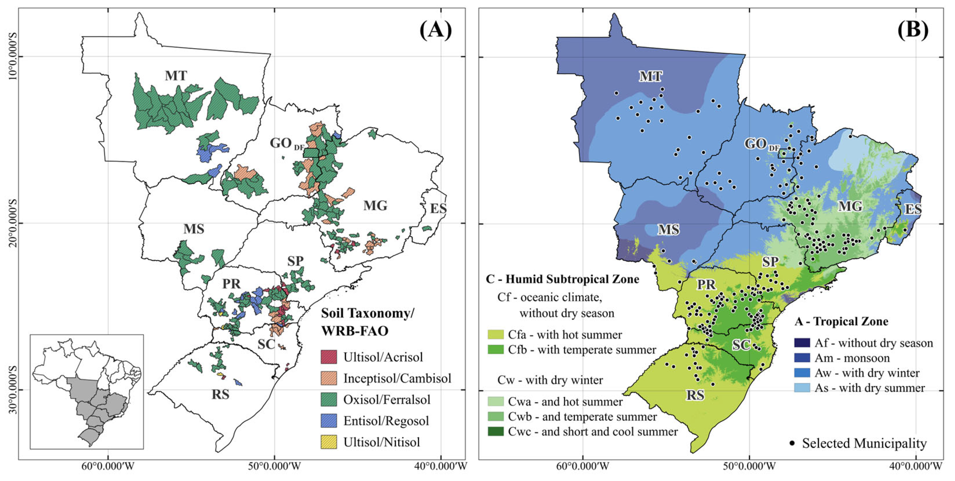
Figure 1. Common bean-producing municipalities selected for this study, their predominant soil classes. The small panel on the left shows the study region in Brazil (A), and the Köppen-Geiger climate classification of the study area (B).
Resources 15 00040 g001
Figure 2. Common bean-producing municipalities during the wet (A) and dry (B) seasons, grouped according to the intensity [mild (0–10%), moderate (>10–30%), intense (>30–70%), or severe (>70–100%)] and timing [early (occurring at the beginning of the sowing window) or late (occurring at the end of the sowing window)] of the maximum observed yield loss.
Resources 15 00040 g002
Figure 3. Simulated common bean yield (kg ha−1) (A,B); functional boxplot of simulated yield (kg ha−1) (C,D); and mean functional yield-loss curves (%) (E,F) for municipalities sown between mid-October and late December during the wet season, classified as moderate and late (blue—A,C,E) or severe and late yield loss (red—B,D,F), as a function of sowing date (day of the year—DOY). The dots in subfigures (A,B) represent the mean yields. Blue and red bands in subfigures (E,F) indicate confidence intervals.
Resources 15 00040 g003
Figure 4. Simulated common bean yield (kg ha−1) (AC); functional boxplot of simulated yield (kg ha−1) (DF); and mean functional yield-loss curves (%) (GI) for municipalities sown between mid-August and late December during the wet season, classified as moderate and early (blue—A,D,G), severe and early (yellow—B,E,H), and severe and late yield loss (red—C,F,I), as a function of sowing date (day of the year—DOY). Dots in subfigures (AC) represent mean yields. The blue, yellow, and red bands in subfigures (GI) indicate confidence intervals.
Resources 15 00040 g004
Figure 5. Simulated common bean yield (kg ha−1) (AC); functional boxplot of simulated yield (kg ha−1) (DF); and mean functional yield-loss curves (%) (GI) for municipalities sown between January and early March during the dry season, classified as intense and late (blue—A,D,G), severe and early (yellow—B,E,H), and severe and late yield loss (red—C,F,I), as a function of sowing date (day of the year—DOY). Dots in subfigures (AC) represent mean yields. The blue, yellow, and red bands indicate confidence intervals.
Resources 15 00040 g005
Figure 6. Simulated common bean yield (kg ha−1) (AC); functional boxplot of simulated yield (kg ha−1) (DF); and mean functional yield-loss curves (%) (GI) for municipalities sown between January and late March during the dry season, classified as intense and late (blue—A,D,G), severe and early (yellow—B,E,H), and severe and late yield loss (red—C,F,I), as a function of sowing date (day of the year—DOY). Dots in subfigures (AC) represent mean yields. The blue, yellow, and red bands indicate confidence intervals.
Resources 15 00040 g006
Figure 7. Radar graph illustrating the characterization of environmental covariates (detailed in Table S7) during the common bean cycle for groups of municipalities with sowing, in the wet season, between October and December (A) and between August and December (B) and, in the dry season, between January and early March (C) and between January and late March (D), classified according to maximum observed yield loss. Points closer to the center of the radar indicate lower values of environmental covariates, whereas points nearer the outer edge indicate higher values. V—vegetative; R—reproductive; FLO—flowering; POD—pod formation; SEED—seed formation; CYCLE—whole crop cycle; and ACC—accumulated. Acronyms for the environmental features (EFs) are described in Figure S7 (Supplementary Materials).
Resources 15 00040 g007
Figure 8. Common bean sowing calendar for groups of municipalities with sowing, during the wet season, between October and December (A) and between August and December (B) and, during the dry season, between January and early March (C) and between January and late March (D), classified according to the maximum observed yield loss. Colors indicate yield-loss categories: 0–10% (mild—green), 10–30% (moderate—yellow), 30–70% (intense—orange), and 70–100% (severe—red).
Resources 15 00040 g008
Disclaimer/Publisher’s Note: The statements, opinions and data contained in all publications are solely those of the individual author(s) and contributor(s) and not of MDPI and/or the editor(s). MDPI and/or the editor(s) disclaim responsibility for any injury to people or property resulting from any ideas, methods, instructions or products referred to in the content.