Article

Towards Transferable Use of Terrain Ruggedness Component in the Geodiversity Index

by
Borut Stojilković
National Education Institute of Slovenia, Poljanska cesta 28, 1000 Ljubljana, Slovenia
Resources 2022, 11(2), 22; https://doi.org/10.3390/resources11020022
Submission received: 30 November 2021 / Revised: 21 January 2022 / Accepted: 7 February 2022 / Published: 14 February 2022
(This article belongs to the Special Issue Geodiversity Assessment: What, Why and How?)

Abstract

:
Geodiversity, as diversity of the abiotic environment, includes terrain ruggedness (or roughness), which is one of the essential parts of geodiversity evaluation. The terrain ruggedness index (R) represents the value of one of the main geodiversity components. The purpose of the study is to discuss the characteristics of R in the scope of geodiversity, and to show how R differs within two specific study areas if we study them using a data scale that covers both areas and only site-specific data. Hence, the main methods include geodiversity element mapping, calculating R based on either the study area or broader-scale data and discussing the differences that arise. The findings show that R should not be calculated only within individual study areas if the results among different study areas are to be compared; rather, it should first be calculated on a larger scale for the whole region in which we are about to compare the specific study areas. The applied value of these results is that such data are then suitable for calculating the geodiversity index (G) according to specific methodological steps and for further analyses.

1. Introduction

Geodiversity, as an abiotic range and expression of variability of geomorphologic, geologic, pedologic, hydrologic, topographic and other characteristics of the environment [1,2,3], has been a subject of study and development for several decades. Many methods have emerged regarding how to calculate the geodiversity index (G) [4], which can be either qualitative [5,6], qualitative–quantitative [7,8,9] or quantitative [3,10,11,12,13]. The latter methods are based on indices and landscape matrixes that combine different aspects and also components of the abiotic environment [4]. They sometimes depend on the purpose of the study [14] or are neutral, and combine the widest range of the abiotic components [15]. Two widely used methods of geodiversity assessment [4,16]—which have also been modified for geodiversity evaluation on micro- [17], mid- and large-scale [18] study areas [17,19] or evaluation purposes [12,20,21]—are the one developed by Pereira et al. [22], which equals the G value to the sum of geological, geomorphological, paleontological, pedological and mineral occurrence sub-indices, and the second one by Serrano and Ruiz-Flaño [3], which divides the multiplication of all geodiversity elements in an area and the terrain ruggedness index (R) of that area with the value of the natural logarithm of the area. The second method, which is to be discussed in greater detail in this article, has been extensively used and applied at various levels—ranging from local [23] to landscape [10] ones—and geographic environments, for example karst [17,24,25] and even the seabed [19], among others. Even though extensive attention has been dedicated to the selection of the geodiversity elements [6], not so many studies discuss the terrain ruggedness (sometimes referred to as roughness [26,27] or rugosity [11]) and its significance in the formula. Ruggedness, which is also used in species distribution studies [28], and had been used for valuing biodiversity prior to geodiversity studies, is used to measure the heterogeneity of the topography, and if its value is larger, it means that the area is more rugged than where the ruggedness values are lower [29].
The terrain characteristics (i.e., its slopes, orientations and, hence, its convexity and concavity [28]) form an integral part of scientific exploration and development in biological studies [30], robotics [31], and other disciplines, as well as when interpreting or valuing either biotic [32] or abiotic environments [33]. When it comes to the abiotic ones, the ruggedness of the terrain becomes explicit, since a plethora of studies gives a special place to the terrain ruggedness when calculating the geodiversity index [11,12,34,35,36]. Namely, they most often multiply the sum of other geodiversity components with the value of R [29], which practically stands for the multiplication of the ruggedness index value and the sum of all other geodiversity elements (e.g., dolines, alluvial fans, lakes) in a block.
The R index by Riley, DeGloria and Elliot [29] has been used extensively, or it has been proposed for such systematic use in various species distribution and other biodiversity studies [37,38,39,40]. It has also been used as a way of including the terrain ruggedness into geodiversity evaluation [3]. It is important because the relief’s ruggedness determines its diversity [26], and is of paramount relevance when interpreting abiotic landscapes in highlands [23,41] as well as in lowlands [26]. Terrain ruggedness has to be included when valuing geodiversity, since the topography affects humidity and sun exposure, as well as erosion and sedimentation processes [42], which is essential for establishing and interpreting the links of geodiversity with biodiversity [43] and climate diversity [44]. It is important to reconsider the position of terrain ruggedness also because the characteristics of digital terrain modeling have evolved in recent decades [45] in order to avoid misinterpretations. Several geodiversity studies [10,26,42] suggest that further studies of ruggedness in terms of geodiversity are needed.
When comparing landscapes in terms of biodiversity, they share a certain level of internal homogeneity [46], which should be taken into account in evaluations and comparisons. The importance of methodological standardization has already been addressed in biodiversity [47,48], which is critical when it comes to ensuring comparability [49]. Even minor differences in protocols bring different results [48]. If the methods are standardized, site data can be put within larger-scale levels and contexts (a regional, landscape or global one) [47]. Similarly, such standardization procedures should be carried out in quantitative geodiversity assessment [16], since geodiversity evaluation has not adopted a unified approach [4]. Unfortunately, present geodiversity evaluation methods are set only for the aims of specific studies [16], which makes their data and results incomparable [50]. That brings out the detail and accuracy as it relates to scale [51]: even if geodiversity assessments are conducted at larger scales and in the same countries (e.g., Brazil [15,22,52]), their results are incomparable because of the absence of connecting data and a unified approach. The comparison possibilities are limited, even on a microscale (e.g., on karst environments [17,23]), if standardized procedures are absent, let alone if the objective is to compare geodiversity on different scale levels of the same area or state (e.g., of Paraná, Brazil [22,36]). That is why common data and methodological steps should be used at specific levels (i.e., global, continental, macro-, meso- and microregional to local [53]) that would cover all the study areas that are potentially to be compared.
Because of these reasons, special attention should be given to what the ruggedness index results show, as well as how and why they differ at different altitudes and among different study areas, if the geodiversity studies are to be standardized, which is one of the main objectives pointed out in the recent studies [54,55,56]. Henceforth, the main aims of the article are:
  • To calculate if there are any differences in the results when calculating R with the same differences between the maximum and minimum values per block at different altitudes;
  • To compare the values of R in two different microregional study areas within one region;
  • To propose a possible standardized way of incorporating the ruggedness component into geodiversity evaluation at different levels.
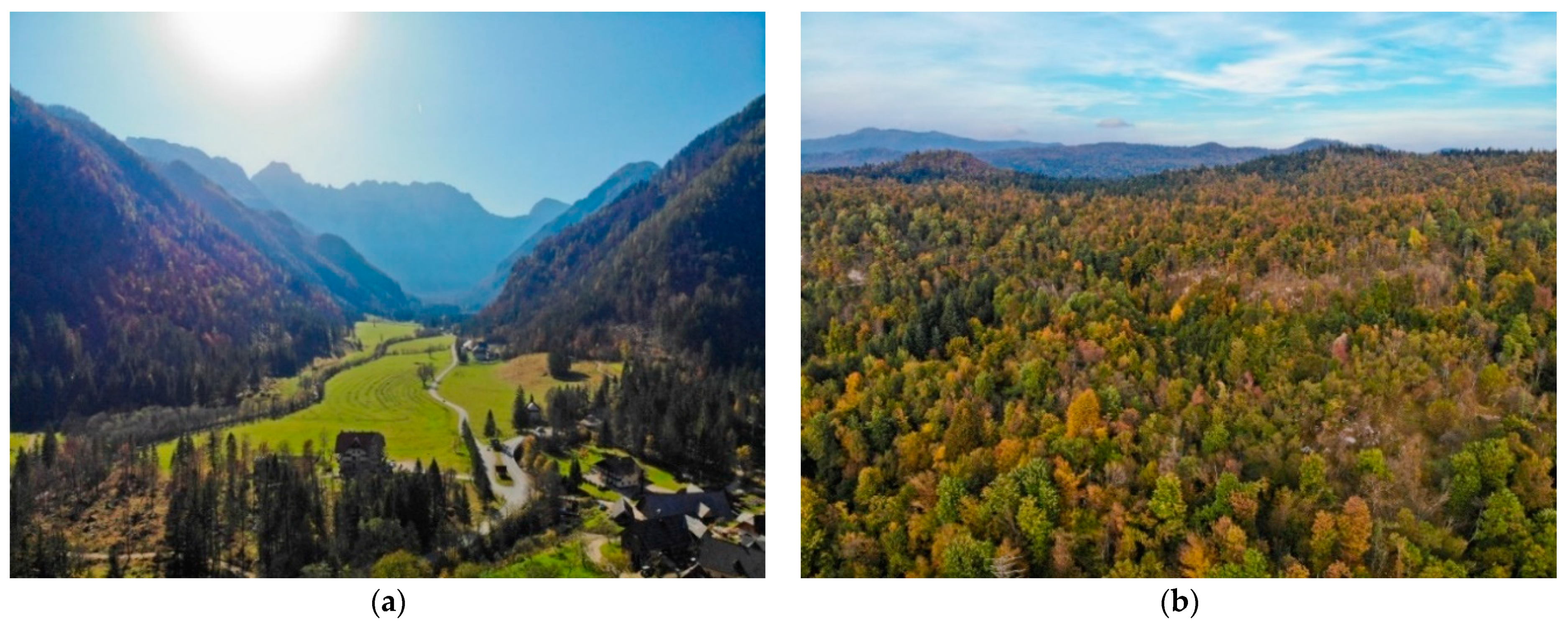
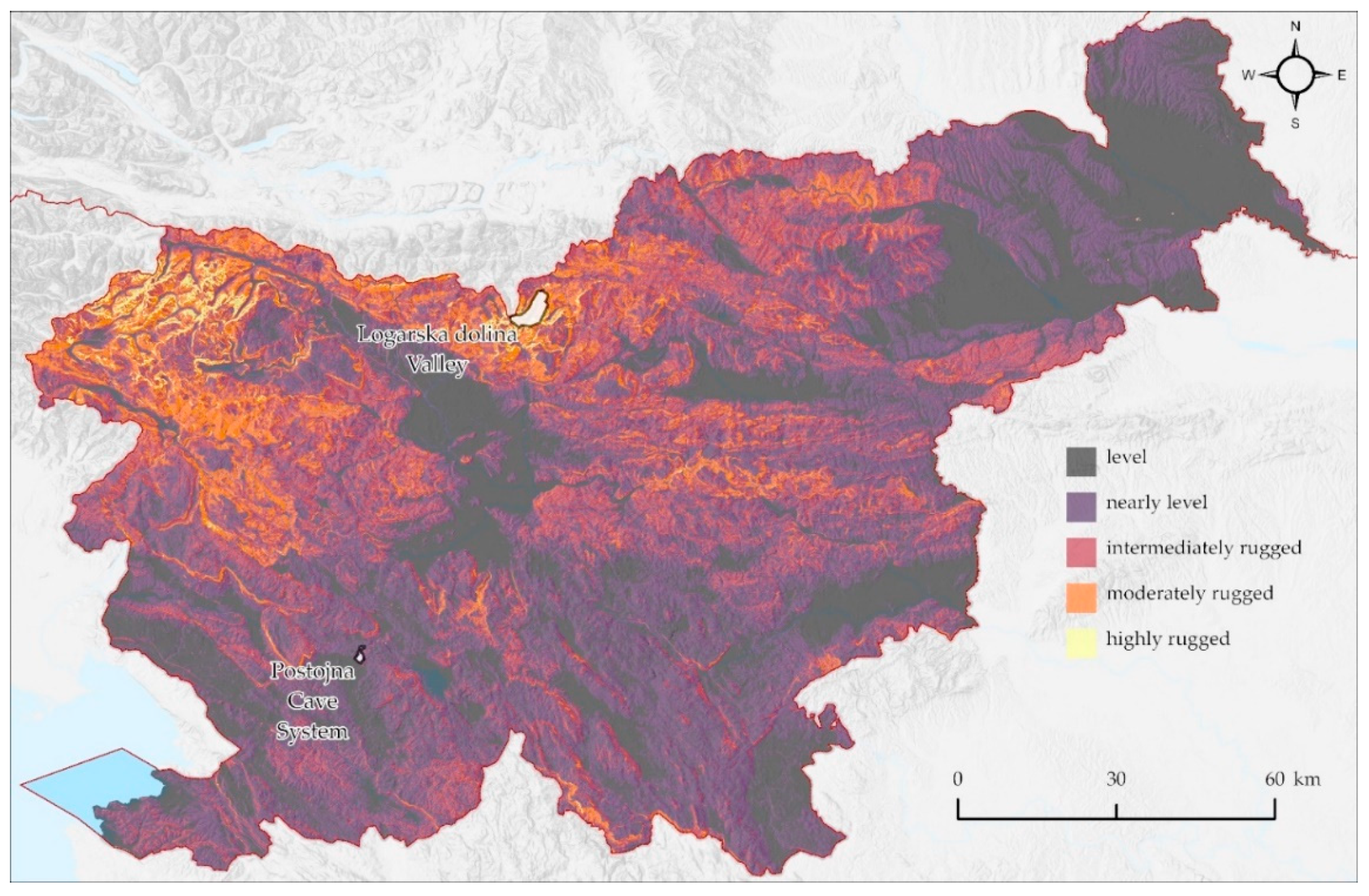
The research niche of the R characteristics in the geodiversity evaluations will be discussed based on the results of using various established geodiversity evaluation methods and procedures [57], which are based on the studies carried out on a classical karst region of the surface area of the Postojna Cave System, and of the Alpine Logar Valley Landscape Park, which underwent glacial and postglacial transformation. Both are situated in Slovenia, Central Europe.

2. Study Areas

Both study areas (Figure 1), the Logar Valley and the surface above the Postojna Cave System, are protected, and they were selected because they are typical representatives of their relief types. They are situated in Slovenia, and serve as a micro-areas of geodiversity evaluation within a greater region—Slovenia.
The Logar Valley is an Alpine valley in the Kamnik–Savinja Alps, which was glacially transformed during the last glaciation [58], and is today one of the key tourist hotspots mainly for hiking and rural tourism. The lateral and terminal moraines of the Logar paleo-glacier are located in the upper part of the valley. Due to its limestone bedrock, there are various smaller caves, springs and shorter creeks that have formed many alluvial fans in the area. The valley floor is filled with glacial and alluvial deposits [59]. Due to its high relief energy, there are many screes and boulder areas beneath numerous cirque systems.
The area of the Postojna Cave System is protected as an area of natural value due to its cave system, as well as its geomorphologic, geologic, hydrologic and biotic characteristics on the surface. The cave system was formed in an Early Cretaceous limestone geologic structure and was influenced by the Postojna anticline. The study area is of 3.42 ha in size [60]. There are numerous caves, dolines, collapse dolines and other typical karst forms and geosites in the area. The area has a small road network and tourism infrastructure, which is extensively used by thousands of tourists annually.

3. Materials and Methods

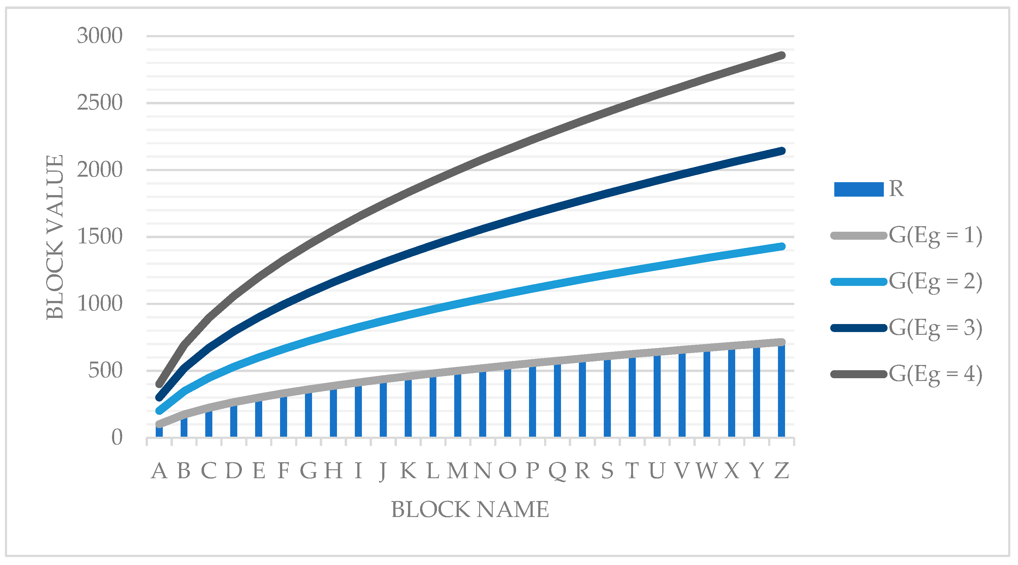
3.1. Calculations of the Ruggedness Index at Different Altitudes

Twenty-six hypothetical blocks were created in the Microsoft Excel environment. In real-life studies, the selection of a certain digital terrain model (DTM)—as well as often also other geodiversity components—depends on the available data [16], which is important to delimit the selection of other geodiversity components. As a hypothetical study, this one is unrelated to block size. Different altitudes were chosen, ranging between the sea level and up to the height of 2600 m. The elevation range within blocks was deliberately the same so that the calculation would show how the values of R differ with altitude. The method, developed by Riley, DeGloria and Elliot [29] was adapted into:
R = | Max 2 Min 2 | ,
where R stands for the ruggedness index, Max is the maximum value (i.e., height above the sea level) and Min is the minimal value per block. The method created by Riley et al. was used because it is often referred to in geodiversity assessments [17,23,41,50,61].
Since often the R values are multiplied with the number of elements per block when calculating G [3], we applied the R values of each block to four different scenarios, where the number of elements per block were ranging from 1 to 4 elements. In this way, we obtained the results and tried to determine whether R differs with altitude and how, in combination with varying number of geodiversity elements, it affects the value of G.

3.2. Form and Size of the Blocks

SAGA-GIS software was used for calculating R, and ArcGIS Pro GIS software was used for all other calculations.
The complete study areas were tessellated with transverse hexagons using the Generate Tessellation tool that subdivided the area in non-overlapping blocks [62], since this options is better than using the squares when determining the neighborhood [63]. Moreover, when using hexagons, the distance between the centers of the neighboring blocks is always the same, and the effect of their border is the smallest among the different geometric shapes [64]. Such block form has already been used in geodiversity assessment [65], since the variations of the distances between the blocks edges and their centers are smaller than with square blocks or equilateral triangles [66]. From the conservation planning point of view, the usage of hexagons results in less fragmented and more efficient portfolios in comparison to rectangular units [67].
The size of the blocks was 10,000 m2, which is the same as if we had used a square block of 100 × 100 m. The reasons for such selection are twofold: the first is that it enables comparisons with other geodiversity evaluations in Slovenia, which use the same surface [50], and the second is that such a size shows differences among the blocks with different numbers of geodiversity components in a way that is neither too fragmented nor too generalized.

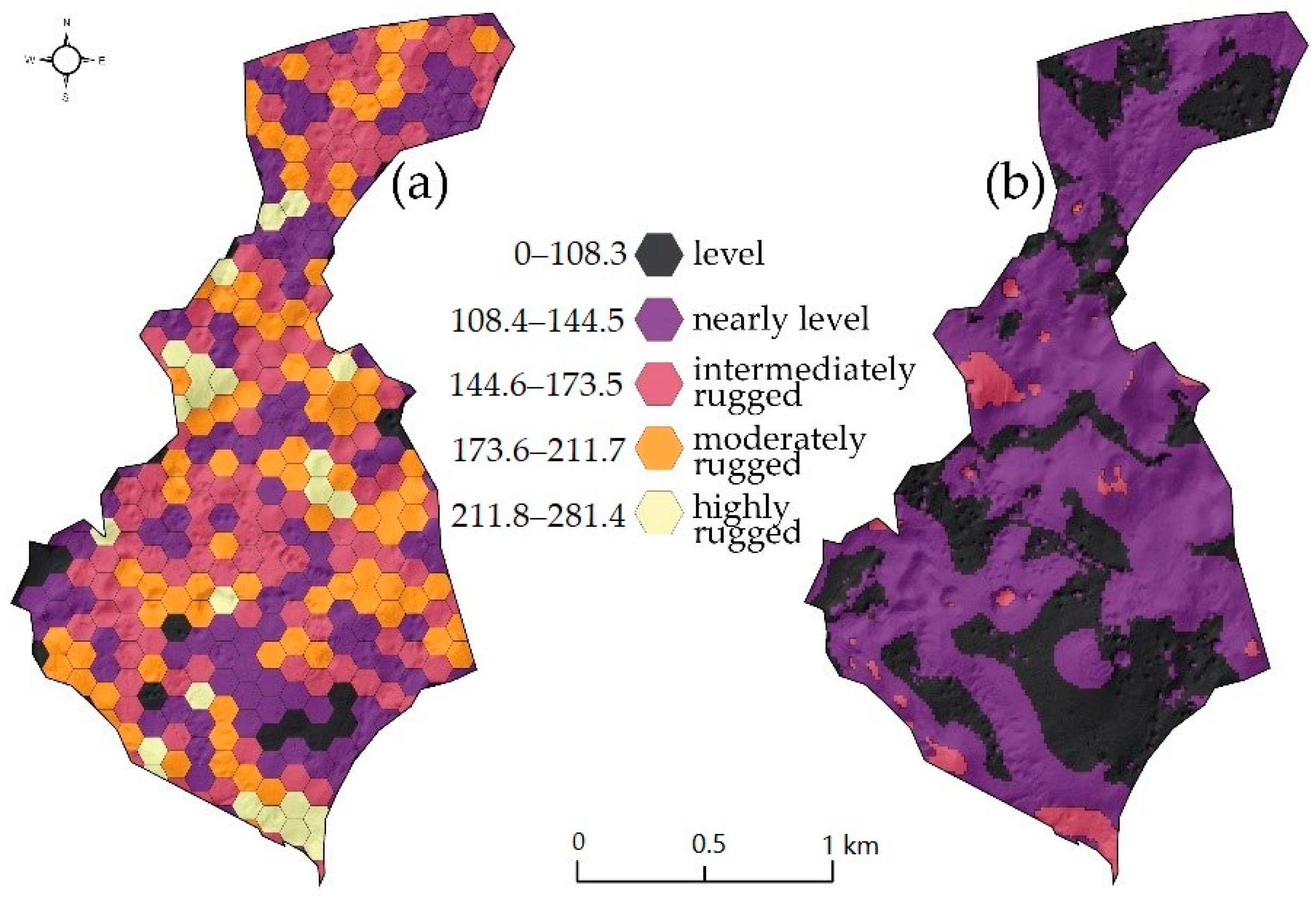
3.3. Calculating Terrain Ruggedness Index

The R index was calculated using a 1 m resolution digital elevation model [68], which was later transformed using the modified formula (Equation 1). Terrain ruggedness composes and affects the value of the geodiversity index, which can be regarded as the topographic element.
Firstly, the lowest and the highest altitudes in specific blocks were determined. Then, both values were used to calculate the ruggedness of the surface [29], using the formula (Equation (1)) described in Section 3.1.
We used a different approach when calculating the index on a higher level. R was calculated for the whole of Slovenia because both study areas are located within it, which makes their results comparable. Different surface processes take place in the areas that belong to different ruggedness classes. That is one of the reasons why different geodiversity elements evolve. Because of that, the proposed method is more suitable than the previously described one.
Using the cubic transformation in ArcGIS Pro, we lessened the resolution of the digital elevation model [68] for the whole of Slovenia; the transformation from 1 m to 5 m was conducted in order to shorten the processing time of calculating R. The second step was calculating R for the whole of Slovenia using SAGA-GIS software and its Terrain Ruggedness Index tool. The analysis was carried out for the radius 100 m and for eight directions. The index was then classified according to Jenks’s method [69], as this is conducted in the majority of quantitative geodiversity evaluation studies. The usual classes, into which the values of the R are classified, are: level, nearly level, slightly rugged, intermediately rugged, moderately rugged, highly rugged and extremely rugged [29]. In order to simplify these classes, we classified the values of R into five ruggedness categories: level, nearly level, intermediately rugged, moderately rugged and highly rugged.
In this way, we calculated the values for every block of cells in the country, which were then used in further calculations.

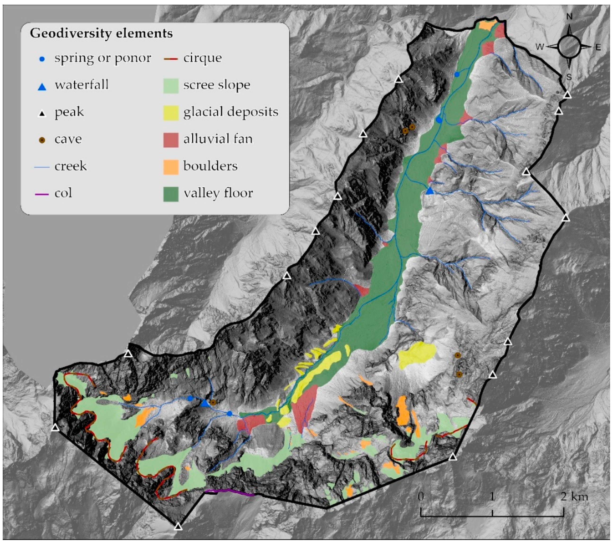
3.4. Mapping Geodiversity Elements

A detailed inventorization of the geomorphologic and hydrologic forms in the study areas was performed using a geomorphologic analytical method [57], and the morphographic map was created using the national topographic map [70], cave database [71] and Lidar data [68], as well as extensive field works in the 2019–2020 period. The morphographic map served as a basis for further spatial analyses.

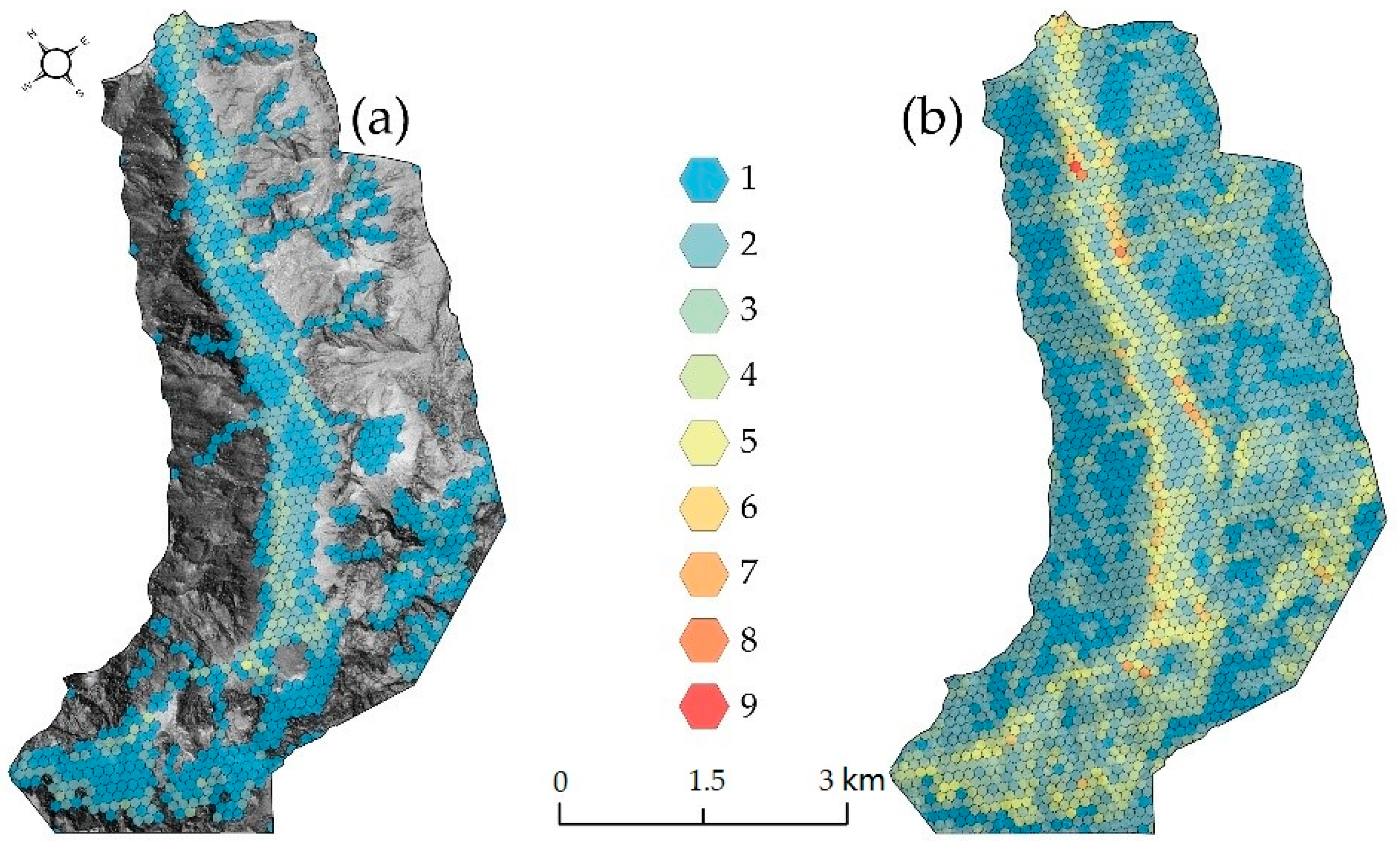
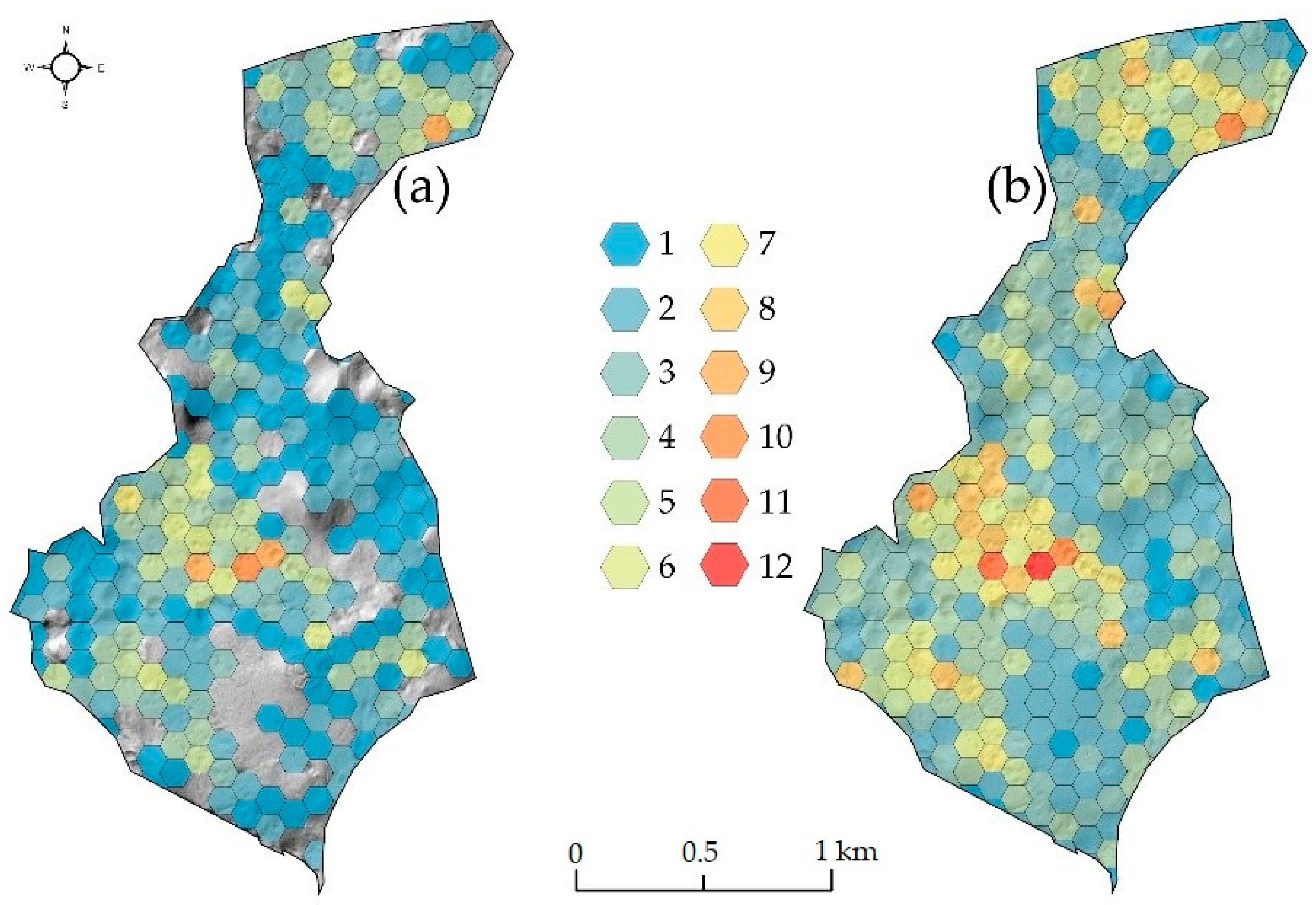
3.5. Calculating Georichness

Georichness, which is also referred to as total geodiversity, is a sum of the geodiversity elements per block [72], and it is, as such, an essential part of geodiversity.
The basic numeric method for calculating G is [3]:
G = E g R ln ( S ) ,
where G represents the geodiversity index, Eg is the number of the geodiversity elements per unit, R is the ruggedness index and ln(S) is the Napierian logarithm of the surface, which regulates the geodiversity value according to the unit area [11]. The formula is regarded as a richness index [18]. Using polygonal units of equal size permits omitting the natural logarithm of the surface area when calculating G:
G = E g R ,
where G represents geodiversity index, Eg is the number of the geodiversity elements per unit and R is the ruggedness index. Such modification has been applied to different study areas [17,23,24].
Only enumerating and summing different geodiversity types does not represent the complexity of geodiversity as a whole [54] since the (un)even distribution of the elements is not included in such a way but only their number per block [73]. That is why further calculations are regarded as georichness (Gr) [72]. Another geodiversity perspective is ‘geoevenness’ (Ge), which remains to be elaborated upon in future research [73].
Since the results in Section 4.1 showed that only multiplying the values of R with the number of other elements per block results in differences if the block is at high or low altitudes, it was decided to calculate the number of different ruggedness classes per block. That procedure outlines the cells with less or more ruggedness classes per block. That is important because, when there are more ruggedness classes in a block, the occurrence of other elements is usually higher. The R classes were used as geodiversity elements, and those classes can be named topographic elements.
G r = E g + E t ,
where Gr represents the georichness value, Eg is the number of the geodiversity elements (geomorphologic, hydrologic, etc.) and Et is the number of topographic elements or ruggedness classes per unit.

4. Results

4.1. Terrain Ruggedness Index at Different Altitudes

In Table 1, the results of calculating index R at different altitudes and the same height difference within blocks are presented. The results vary: block A, with its minimum value at sea level (0 m) and its maximal value 100 m above it, has the R value of 100; block B, being situated in the area of the same elevation range, but between the altitudes of 400 and 500 m above sea level, has higher R values (300). Block C has even higher altitudes that vary from 900 to 1000 m above sea level; thus, analogically, R values are even higher. This simple calculation shows that the R values change with the distance above sea level, even if the height difference per block remains the same. These results have a great impact on the G index as well: namely, the ruggedness value is multiplied by the number of the elements in that block [3], which results in differences among the blocks at different altitudes, even if they have the same number of geodiversity elements within them.
Figure 2 further elaborates on the topic, as it shows the difference among the R values in relation to the number of geodiversity elements per block. Here, 26 hypothetical blocks (A–Z) underwent a calculation of G in four different scenarios (i.e., with Eg values varying from 1 to 4). The results support Gray’s claim [74] that one of the geodiversity hotspots is in high mountain areas, but the reason for this is numerically in the elevation itself. Whether the variability of the geodiversity elements is bigger at higher altitudes in comparison to lower altitudes is a question of further research. The results of the calculations show that both R and G increase with the altitude, even if the difference in block maximum and minimum values is the same.

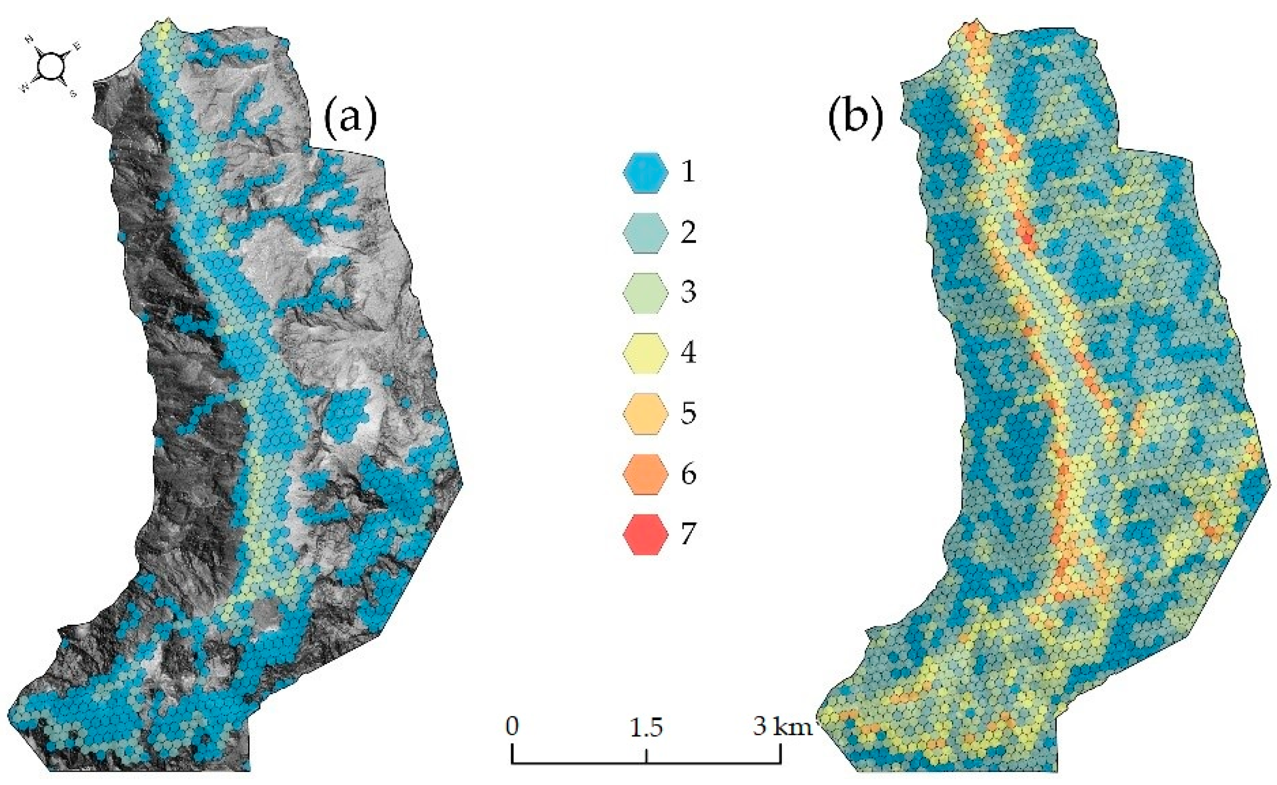
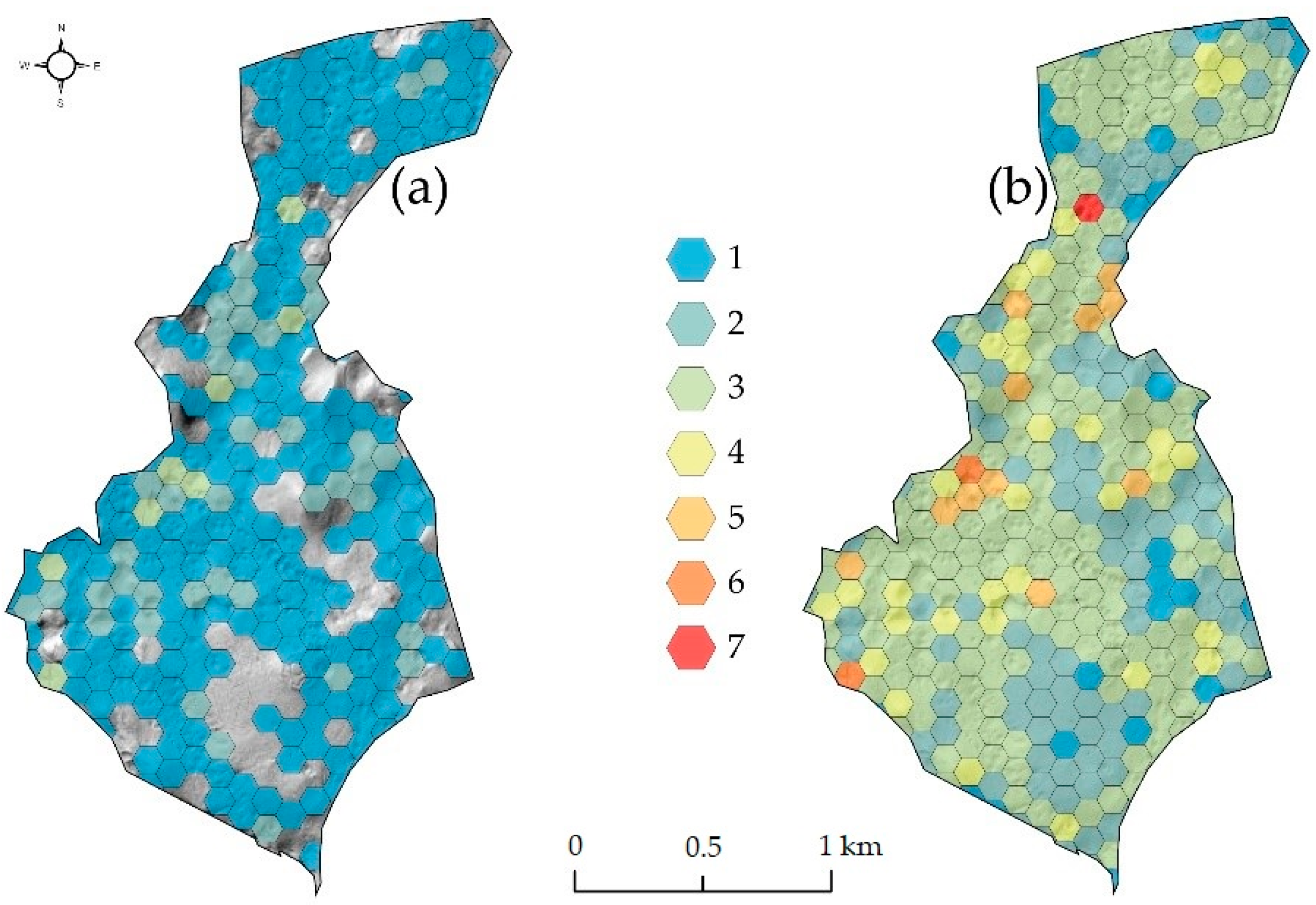
4.2. Terrain Ruggedness Index of Different Study Areas within Specific Regions

The theoretical results of Section 4.1 can be illustrated in both of the actual study areas: the Postojna Cave System protected area is situated at lower altitudes in the classical karst region of Slovenia, and has much smaller height differences at the same distances in comparison to the Logar Valley Landscape Park, which is situated in the Alpine region. Due to that, theoretically, if the R of a block with the same height difference would be calculated in both areas, the result would be higher in the Logar Valley because of its higher altitude.
To calculate the georichness values of the blocks in both areas, we summed the mapped geodiversity elements with the number of R classes that were present in a specific block. As presented in Figure 3, the surface is highly rugged in the high mountain areas of the Julian Alps and the Kamnik–Savinja Alps in the north of the country. It is moderately rugged in the mountainous areas as well, and also in the pre-Alpine area (central Slovenia), as well as in some smaller parts of the Dinaric mountains (central west to southeast Slovenia). Intermediately rugged surfaces encompass the pre-Alpine and Dinaric regions with intermediate ruggedness characteristics. Nearly level and level areas are typical of the greater lowlands, basins and specifically for sub-Pannonian Slovenia in the east of the country.
Each ruggedness class has its predominant physical geographic processes and characteristics that result in typical landforms and other abiotic environmental characteristics. For example, cirque systems are in the areas of highly rugged topography, and alluvial terraces are predominantly in the areas of level topography, but not vice versa. Even if there are no major morphographic or hydrologic forms in an area (e.g., on a slope), that area has its own predominant process (e.g., denudation), which results in specific terrain ruggedness characteristics. Because of that, the classes of the ruggedness index R can be used as specific geodiversity elements when calculating G.
The Logarska dolina Valley, or the Logar Valley, is a typical Alpine valley with a very big difference between the highest and the lowest ruggedness values. It encompasses a level area at the valley floor, as well as areas with big relief energy, which results in a highly rugged surface. The in-between values are consecutively distributed between the level and highly rugged areas, mainly on the valley slopes. However, as seen in Figure 4, the R values per block in study area (a) differ greatly from the R values of Slovenia (b): the differences are mainly visible at the valley bottom, where more blocks are in the lowest class, and on the valley slopes, where there are far more nearly level and intermediately rugged areas than in calculation (b).
If R is calculated for Slovenia and compared to the results, and if R is collected only within the study areas (Figure 4), the slopes of the Logar Valley mainly appear to be moderately rugged in comparison to other slopes in the country, which is the greatest difference of both calculations. However, there is only a slight difference with the highly rugged areas that are located where the slope inclination is the biggest (i.e., in the areas of the cirques and scree slopes, as seen in Figure 5 [41]).
The differences in values are even more obvious for a classical karst landscape in Slovenia, where the relief energy is lower than in the Logar Valley. When R is calculated only for the study area (Figure 6a), the values are distributed in all five classes; in that case, the surface is level only in some spots, where there are either no geomorphologic surface forms in the block areas, or if those elements are bigger than the blocks themselves (e.g., a blind valley, which can be seen in Figure 7). The values of R in calculation (a) are distributed depending on the maximum and minimum elevation values per block within the study area. The highest values are at the hill tops and in the area of contact with the karst at the south, as derived from Figure 7.
The values for R in scenario (b) in the protected area of the Postojna Cave System are distributed differently: at the country level, this study area is mainly level to nearly level, which is a much more realistic image, since there are no high slopes or height differences in the study area (as visible in Figure 1b). The surface is intermediately rugged only at the contact points of different relief types (in the south), or where bigger dolines or higher peaks of the hills are situated. However, if R is calculated only within this study area (Figure 6a), some parts of the area are moderately or even highly rugged, which is a drastic discrepancy with the values of the same R classes in the Logar Valley Landscape Park (Figure 4a).

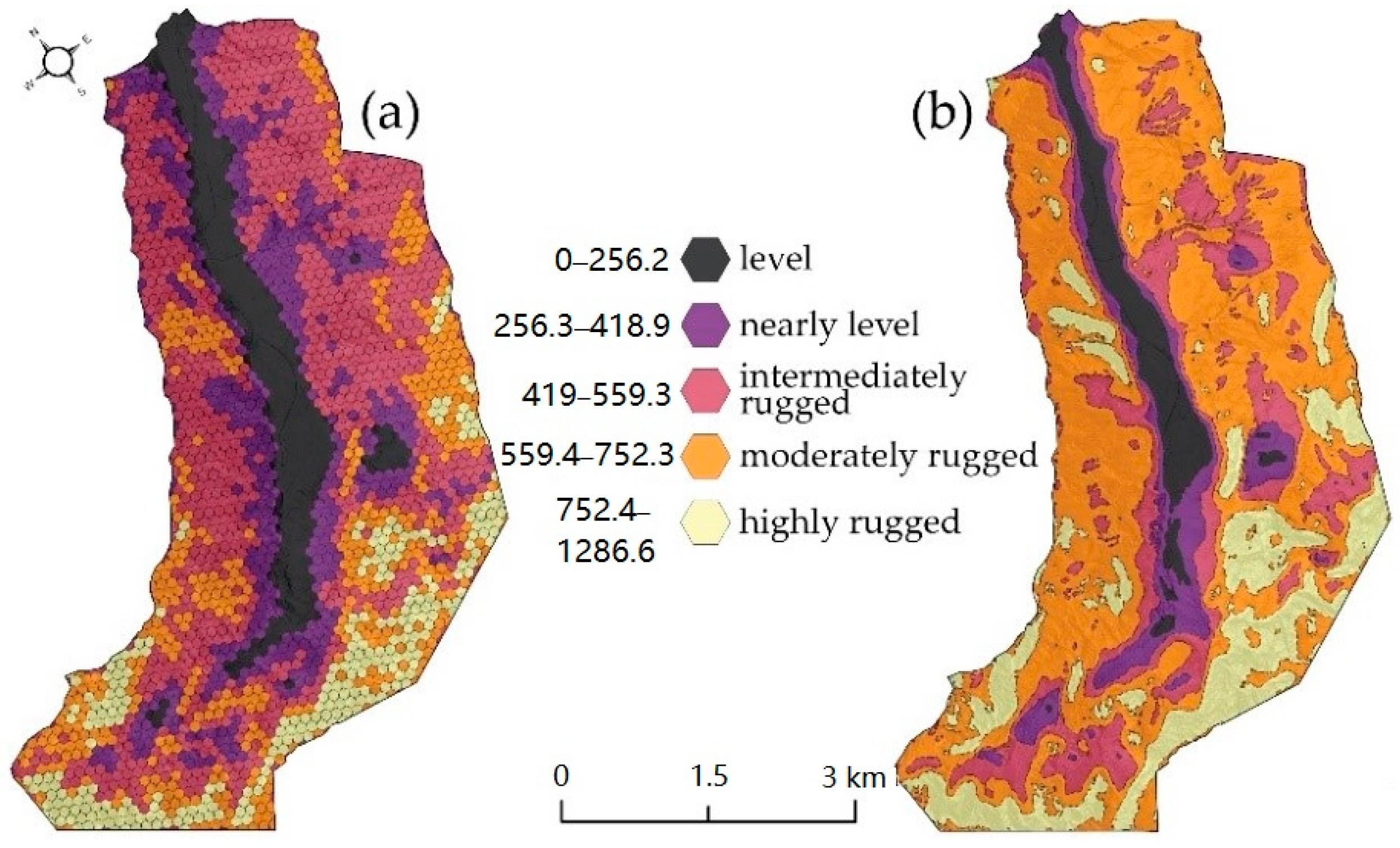
4.3. Terrain Ruggedness Classes as Geodiversity Elements

The purpose of this article is to show how the values of the ruggedness can affect the geodiversity index values. That is why only selected main geodiversity elements were chosen and mapped for both study areas, which are mainly geomorphologic and hydrologic.
The Logar Valley was glacially transformed in the LGM [59], which is reflected in the cirques and glacial deposits (moraine material). Other geodiversity elements in the areas are linked to its limestone and dolomite bedrock [75] and differences in slope steepness: the scree slopes and boulder areas are located in the vicinity of cirque systems, the creeks (36) are either on the valley slopes or at the bottom between springs (four), waterfalls (two) and ponors (one); 11 alluvial fans are located in the intermediately rugged areas at the contact points between the slopes and valley floor. Moreover, 15 peaks are distributed on the valley ridges, as is the biggest col and the cave entrances to smaller caves (four) on both slopes [41]. Since both the scree slope material and the boulders are of the same genetic origin, we considered them as one geodiversity element in further calculations.
The Postojna Cave system is a protected area due to its limestone structure, which is dominated by typical karst landforms: numerous collapse dolines, cave entrances and other forms are linked to past and present geomorphic subsurface processes [76]. There are 331 dolines, 18 collapse dolines and 15 karst peaks; there are also two shorter creeks with springs and ponors, and one blind valley in the SW of the area. The dolines are distributed in four NW to SE stripes, which are separated by areas of collapse dolines and peaks.
The next procedural step was calculating the total number of elements per block. That was performed for both study areas twice, by omitting (a) or including (b) the number of different ruggedness classes in each block, as presented in Figure 8 and Figure 9.
The total number of the elements per block in the Logar Valley in scenarios (a) and (b) is the highest in the area of the valley floor and its contact with other elements (e.g., creeks, alluvial fans). If we omit the ruggedness, the highest number of elements per block is six, but if we add the ruggedness classes, it is nine. In both cases, the highest number is at the contact point of springs, creeks and various topographic changes in the north of the valley. If ruggedness is omitted, there are no elements in the slopes where no other major elements are mapped. However, if the topographic element is added, the values of those blocks vary because the terrain ruggedness varies within the same slopes as well, depending on the height difference in each block.
The total number of elements per block in the protected area of the Postojna Cave System differs as well if we compare scenarios (a) and (b) (Figure 9). When ruggedness is not included (Figure 9a), the total number of elements per block is ten, which is the case with only one block, where ten dolines are located. Another extreme is value one, where only one geodiversity element is located. Where no geodiversity elements were mapped, the value is zero. The higher values are in two types of areas: with the higher numbers of mainly dolines, or dolines in combination with other geomorphologic elements. In contrast, if the topographic elements are added (Figure 9b), the maximum value is twelve and the minimum is one. The latter is in blocks with only one topographic element. The similarity among both scenarios is that the higher values are in the blocks with the higher number of elements. However, in the scenario (b), those blocks are more evenly distributed throughout the study area. From the richness perspective, the highest value has the central part of the area, where the topographic classes vary in combination with many other geodiversity elements.
The diversity of elements (Figure 10 and Figure 11) is different from the total number of the elements (Figure 8 and Figure 9). ’The diversity of elements’ includes different geodiversity elements and not their absolute numbers (e.g., if there are three springs in a block, that is only one geodiversity element).
As visible in Figure 10, if we omit the ruggedness classes (i.e., the topographic elements), the maximum value of the geodiversity elements in the Logar Valley is four, which is in the north where boulders, the alluvial valley floor, the alluvial fan and a creek meet in one block. Since this area is not rugged, it does not have the highest diversity values. The blocks with the highest diversity values are at another location: at the contact point of the valley floor and slope at the eastern and western sides of the valley. In those areas, there are different geomorphologic, hydrologic and topographic elements within a specific block. Such a case is at the eastern slope of the valley, where the highest number of elements per block is seven.
The results of the diversity calculation for the karst study area show different values to the richness calculations. The maximum diversity of the element types per block without ruggedness classes is three, and with ruggedness classes, it is seven. As regards the topographic elements, there are only three different geodiversity elements per block (e.g., a doline, a cave and a peak); in other blocks, there are either two elements, one element (mainly a doline) or there are no elements. When adding different ruggedness classes, the range is from one to seven element types per block: one element is only in the blocks where only one topographic element was located, whereas the highest number of different elements is in the blocks, where different topographic classes are combined with different geomorphologic–hydrologic elements. That block is also the most geodiverse. Including the topographic elements to G leads to higher values of G, especially if the differences in height per block are high in comparison to areas where the surface is level and the differences in height are low.

5. Discussion

Topography is most often the basis of the landform classification [26], and topographical heterogeneity can be quantified objectively using a terrain ruggedness index [29]. Whether used as such or adapted, it has been used in quantitative geodiversity evaluations [17,41,50,61] that are based on the method that explicitly relates to the ruggedness index [3]. The research problem of this article is to investigate the characteristics and influence of the terrain ruggedness index (R) developed by Riley, DeGloria and Elliot [29] in the scope of the geodiversity index (G) by Serrano and Ruiz-Flaño [3]. Following the established methodological procedure of calculating R and G [12,17,39,61], the three aims of the article were completed. Most importantly, a standardized way of incorporating the ruggedness component or the topographic element (Et) into geodiversity was proposed and elaborated upon. It is essential to keep the ruggedness component included in geodiversity because it has an effect on the formation and distribution of other elements, and it shows specific terrain characteristics [77].
The results of multiplying the terrain ruggedness index values with the sum of other geodiversity elements [3] help to distinguish the areas with high and low G index values: theoretically, the G values will be the highest if the R values are high and the sum of other geodiversity components is high as well; the values will be lower if the area encompasses either a smaller number of geodiversity components and high values of R, or lower values of R and a bigger number of other geodiversity components. The G values will be the lowest in the areas that are both level or only slightly rugged, and with a smaller number of other geodiversity components.
The first major finding of the research is that the R values increase with altitude, even if the difference between the minimum and maximum elevation value in a block remains the same. If a block with a specific height difference within it is located at the sea level, its R value will be smaller than if the block with the same height difference is anywhere else above the sea level. When the R values are multiplied with the number of other geodiversity elements within that block, the differences become even greater. This simple calculation shows that a block in an area of high altitude automatically has a higher value when calculating either R or G, regardless of its terrain characteristics. This is one of the reasons why the R and G calculation methods should be adapted to a certain methodology in order for the results to be comparable when valuing the geodiversity of different areas. The added value of such a standardized procedure would become useful, for example, in any environmental protection process, which is one of the aims of valuing geodiversity [78], or when comparing the geodiversity of different areas following the same method, which has been problematic, since no standard geodiversity evaluation procedure has been either agreed upon or widely used [4].
As shown in the cases of classical karst and Alpine areas, the R values differ when the index is calculated within the areas. The R values of a classical karst landscape in Slovenia are much lower than those of the mountainous area, which is reasonable to expect in advance. However, if those values are classified in any way, the classes become incomparable, since the karst area does not have as rugged surfaces as the mountainous area. The input data of different study areas and evaluation methodologies should be standardized [4,79] in order for the results to be comparable. Besides using the input data of the same quality and the same expert-based data regarding geodiversity components and elements selection, one of the possible links is the ruggedness component, which has to be calculated in a region such that it covers all the study areas in which we want to compare the G values. The region in which R is calculated has to be at a higher spatial level than the study areas, and it also has to include the data of all study areas, as it has been demonstrated in this article, where R was calculated at a higher level than the one at which the study areas are: we calculated R for the whole of Slovenia and then used it at a micro level in both study areas. That is analogical to biodiversity comparisons of different areas on a global level, where comparative and standardized data and methods are essential, even if the study areas are on different continents [49].
Table 2 provides a multilevel theoretical comparison of four regions (X, Y, W and Q) and the study areas distributed within them at different levels, which could be one of the guidelines for a standardized ‘geodiversity assessment toolkit’ creation [16]. If two study areas are located within one region (e.g., A1,1 and A1,2), R has to be calculated for the whole region where they are situated (in this case Region X). That is the rule in the cases either if we want to value the geodiversity of the areas separately, or if we want to compare the values of both indices. That has been demonstrated in this article, where Region X is Slovenia and the study areas are at level A. If the study areas are located in two regions, R has to be calculated with common data for both regions (level B). If there are three or more study areas in at least three regions, then R has to be calculated for all three regions (level C) and so forth.
Another question that remains to be answered is the purpose of the geodiversity evaluation. If it is to compare the G values, then the index should be tailored adequately, as shown in Table 2. If there is the potential for an ongoing research where study areas will be added, then it is sensible to calculate R at the beginning at a higher spatial level. However, if the purpose of the geodiversity evaluation is a special one (e.g., for geotourism [25,80,81,82], educational [24,83,84] or other) within one set area, then it is not necessary to use data from higher levels that would also encompass other areas.
The terrain ruggedness determines the diversity of the relief [26]. When R was calculated at a state level, big differences of the values in both study areas emerged: the karst area was much more level than the mountainous one. When the results were classified, specific classes were considered to be topographic geodiversity elements (Et). The two most widely applied methods of calculating G have a fundamental difference: one multiplies the geodiversity elements with the ruggedness index value [3], whereas the other one sums various subindices in order to obtain the G value [22]. One methodological development is to integrate the strong points of both methods: the R values which definitely impact geodiversity [74] can be classified in set classes according to Jenks’s classification [69] at a specific level (derived from the method of Serrano and Ruiz-Flaño [3]) and, as such, can be added (not multiplied) as topographic elements to other geodiversity elements (as it is the case with the method of Pereira et al. [22]). In that way, the georichness of an area is calculated in a much more comparable way to the value of the same parameter types of different areas. If the georichness is calculated in this way, the results become comparable: the quality of data is the same (the same resolutions of DEM and boundaries for the ruggedness classes are used, as are the same expert-based criteria for geodiversity components and elements selection). This is the same with the diversity of the elements: if this method is applied, the complete study areas become covered with at least one element, and their diversity can be compared (as seen in Figure 10 and Figure 11).

6. Conclusions

The principle of an objective comparison of the results is among the most important ones when valuing geodiversity. When using common topographic data, selecting geodiversity elements of the same type and following standard methodologies, it is possible to compare the geodiversity index values of different areas. The first conclusion is that the ruggedness index is methodologically designed in a way that areas of high altitude will have higher ruggedness index values. When it comes to valuing the geodiversity of different study areas, the terrain ruggedness index becomes one of the main elements and factors of the calculation, and should remain so if the geodiversity of two or more areas are compared using an index-based approach. As such, it should be classified, and the classes should be regarded as topographic elements where specific abiotic processes happen. If not—as shown in the article—the ruggedness index values have a too big impact on the geodiversity index values.
Another essential fact to be taken into consideration when calculating the ruggedness index is that it should be calculated transparently at a level that encompasses all study areas in order for the results to be comparable and transferable (e.g., at least on a country level, if there are various studies for different locations within it). The significance of this idea responds to various studies that have pointed out that geodiversity evaluation methodology should be standardized [4,79] in a methodological way, as well as according to the selection of elements (or materials) used in the evaluations.
Future research directions of the methodological development of the geodiversity index should be oriented towards further studies of not only the ruggedness component of the established methods, but also the precise and objective selection of all geodiversity elements. The studies that have already been conducted on this field [6] should be brought together for different relief and landscape types and, as such, they should be standardized [16]. Furthermore, the abiotic and biotic diversities of different areas should be comparable [55], which is why the methods for their assessment ought to be standardized. Another path that the methodological development of assessing geodiversity should take is incorporating other components of the landscape metrics into the geodiversity index [32,46], not only to assess the richness of the elements, but also their even distribution.
The method for calculating the ruggedness index for geodiversity evaluation proposed in the study is applicable to any study area, regardless of its size or intrinsic geographic characteristics. Due to that, the results and the message of this study provide a contribution to the methodological development of valuing geodiversity and, as such, provide a means for further methodological development in valuing the environment holistically and objectively.

Funding

Not applicable.

Institutional Review Board Statement

Not applicable.

Informed Consent Statement

Not applicable.

Data Availability Statement

Not applicable.

Acknowledgments

The author would like to thank the editor, Paulo Pereira, for valuable suggestions when writing the manuscript, as well as to anonymous reviewers for thorough review and meaningful insights into the topic. Special thanks go to Sašo Stefanovski for the help with cartography.

Conflicts of Interest

The author declares no conflict of interest.

References

  1. Nieto, L.M. Geodiversidad: Propuesta de una definición integradora. Boletín Geológico Min. 2001, 112, 3–12. [Google Scholar]
  2. Gray, M. Geodiversity: Valuing and Conserving Abiotic Nature; John Wiley & Sons Ltd.: Chichester, UK, 2004; ISBN 1118525094. [Google Scholar]
  3. Serrano, E.; Ruiz-Flaño, P. Geodiversity: A theoretical and applied concept. Geogr. Helv. 2007, 62, 140–147. [Google Scholar] [CrossRef]
  4. Zwoliński, Z.; Najwer, A.; Giardino, M. Methods for Assessing Geodiversity. In Geoheritage; Reynard, E., Brilha, J., Eds.; Elsevier: Amsterdam, The Netherlands, 2018; pp. 27–52. [Google Scholar] [CrossRef]
  5. Panizza, M. The geomorphodiversity of the Dolomites (Italy): A Key of geoheritage assessment. Geoheritage 2009, 1, 33–42. [Google Scholar] [CrossRef] [Green Version]
  6. Bradbury, J. A keyed classification of natural geodiversity for land management and nature conservation purposes. Proc. Geol. Assoc. 2014, 125, 329–349. [Google Scholar] [CrossRef]
  7. Benito-Calvo, A.; Pérez-González, A.; Magri, O.; Meza, P. Assessing regional geodiversity: The Iberian Peninsula. Earth Surf. Process. Landforms 2009, 34, 1433–1445. [Google Scholar] [CrossRef]
  8. Argyriou, A.V.; Sarris, A.; Teeuw, R.M. Using geoinformatics and geomorphometrics to quantify the geodiversity of Crete, Greece. Int. J. Appl. Earth Obs. Geoinf. 2016, 51, 47–59. [Google Scholar] [CrossRef] [Green Version]
  9. Zakharovskyi, V.; Németh, K. Quantitative-qualitative method for quick assessment of geodiversity. Land 2021, 10, 946. [Google Scholar] [CrossRef]
  10. Hjort, J.; Luoto, M. Geodiversity of high-latitude landscapes in northern Finland. Geomorphology 2010, 115, 109–116. [Google Scholar] [CrossRef]
  11. Pellitero, R.; González-Amuchastegui, M.J.; Ruiz-Flaño, P.; Serrano, E. Geodiversity and Geomorphosite Assessment Applied to a Natural Protected Area: The Ebro and Rudron Gorges Natural Park (Spain). Geoheritage 2011, 3, 163–174. [Google Scholar] [CrossRef]
  12. Melelli, L. Geodiversity: A New Quantitative Index for Natural Protected Areas Enhancement. Geoj. Tour. Geosites 2014, 13, 27–37. [Google Scholar]
  13. Kot, R. The point bonitation method for evaluating geodiversity: A guide with examples (Polish Lowland). Geogr. Ann. Ser. A Phys. Geogr. 2015, 97, 375–393. [Google Scholar] [CrossRef] [Green Version]
  14. Melelli, L.; Vergari, F.; Liucci, L.; Del Monte, M. Geomorphodiversity index: Quantifying the diversity of landforms and physical landscape. Sci. Total Environ. 2017, 584–585, 701–714. [Google Scholar] [CrossRef] [PubMed]
  15. de Paula Silva, J.; Rodrigues, C.; Pereira, D.I. Mapping and Analysis of Geodiversity Indices in the Xingu River Basin, Amazonia, Brazil. Geoheritage 2015, 7, 337–350. [Google Scholar] [CrossRef] [Green Version]
  16. Crisp, J.R.A.; Ellison, J.C.; Fischer, A. Current trends and future directions in quantitative geodiversity assessment. Prog. Phys. Geogr. 2021, 45, 514–540. [Google Scholar] [CrossRef]
  17. Stepišnik, U.; Trenchovska, A. A New Quantitative Model for Comprehensive Geodiversity Evaluation: The Škocjan Caves Regional Park, Slovenia. Geoheritage 2018, 10, 39–48. [Google Scholar] [CrossRef]
  18. Pellitero, R.; Manosso, F.C.; Serrano, E. Mid- and Large-Scale Geodiversity Calculation in Fuentes Carrionas (NW Spain) and Serra do Cadeado (Paraná, Brazil): Methodology and Application for Land Management. Geogr. Ann. Ser. A Phys. Geogr. 2015, 97, 219–235. [Google Scholar] [CrossRef]
  19. Kaskela, A.M.; Kotilainen, A.T. Seabed geodiversity in a glaciated shelf area, the Baltic Sea. Geomorphology 2017, 295, 419–435. [Google Scholar] [CrossRef]
  20. Bétard, F.; Peulvast, J.P. Geodiversity Hotspots: Concept, Method and Cartographic Application for Geoconservation Purposes at a Regional Scale. Environ. Manag. 2019, 63, 822–834. [Google Scholar] [CrossRef]
  21. Perotti, L.; Carraro, G.; Giardino, M.; De Luca, D.A.; Lasagna, M. Geodiversity Evaluation and Water Resources in the Sesia Val Grande UNESCO Geopark (Italy). Water 2019, 11, 2102. [Google Scholar] [CrossRef] [Green Version]
  22. Pereira, D.I.; Pereira, P.; Brilha, J.; Santos, L. Geodiversity assessment of Paraná State (Brazil): An innovative approach. Environ. Manag. 2013, 52, 541–552. [Google Scholar] [CrossRef] [Green Version]
  23. Trenchovska, A.; Stojilković, B. Geodiverziteta Narodnega parka Severni Velebit. In Dinarski kras: Severni Velebit; Stepišnik, U., Ed.; Znanstvena založba Filozofske fakultete Univerze v Ljubljani: Ljubljana, Slovenia, 2019; pp. 108–124. [Google Scholar] [CrossRef]
  24. Stepišnik, U.; Ilc Klun, M.; Repe, B. Vrednotenje izobraževalnega potenciala geodiverzitete na primeru Cerkniškega polja. Dela 2017, 2017, 5–21. [Google Scholar] [CrossRef] [Green Version]
  25. de Sena, Í.S.; de Ruchkys, Ú.A.; Travassos, L.E.P. Geotourism Potential in Karst Geosystems: An example from the Lund Warming Ramsar Site, Minas Gerais, Brazil. Catena 2022, 208, 1–10. [Google Scholar] [CrossRef]
  26. Kot, R.; Leśniak, K. Impact of different roughness coefficients applied to relief diversity evaluation: Chełmno Lakeland (Polish Lowland). Geogr. Ann. Ser. A Phys. Geogr. 2017, 99, 102–114. [Google Scholar] [CrossRef]
  27. Năpăruş-Aljančič, M.; Pătru-Stupariu, I.; Stupariu, M.S. Multiscale wavelet-based analysis to detect hidden geodiversity. Prog. Phys. Geogr. 2017, 41, 601–619. [Google Scholar] [CrossRef]
  28. Olsen, A.C.; Severson, J.P.; Allred, B.W.; Jones, M.O.; Maestas, J.D.; Naugle, D.E.; Yates, K.H.; Hagen, C.A. Reversing Tree Encroachment Increases Usable Space for Sage-Grouse during the Breeding Season. Wildl. Soc. Bull. 2021, 45, 488–497. [Google Scholar] [CrossRef]
  29. Riley, S.J.; DeGloria, S.D.; Elliot, R. A Terrain Ruggedness Index that Qauntifies Topographic Heterogeneity. Intermt. J. Sci. 1999, 5, 23–27. [Google Scholar]
  30. Xiong, Y.; Li, Y.; Xiong, S.; Wu, G.; Deng, O. Multi-scale spatial correlation between vegetation index and terrain attributes in a small watershed of the upper Minjiang River. Ecol. Indic. 2021, 126, 107610. [Google Scholar] [CrossRef]
  31. Zhang, Z.; Wang, L.; Liao, J.; Zhao, J.; Zhou, Z.; Liu, X. Dynamic stability of bio-inspired biped robots for lateral jumping in rugged terrain. Appl. Math. Model. 2021, 97, 113–137. [Google Scholar] [CrossRef]
  32. El Hasnaoui, Y.; Mhammdi, N.; Bajolle, L.; Nourelbait, M.; Bouimetarhan, I.; Cheddadi, R. Locating North African microrefugia for mountain tree species from landscape ruggedness and fossil records. J. African Earth Sci. 2020, 172, 103996. [Google Scholar] [CrossRef]
  33. Shetty, S.; Umesh, P.; Shetty, A. Dependability of rainfall to topography and micro-climate: An observation using geographically weighted regression. Theor. Appl. Climatol. 2022, 147, 217–237. [Google Scholar] [CrossRef]
  34. Martinez-Graña, A.M.; Goy, J.L.; Cimarra, C. 2D to 3D geologic mapping transformation using virtual globes and flight simulators and their applications in the analysis of geodiversity in natural areas. Environ. Earth Sci. 2015, 73, 8023–8034. [Google Scholar] [CrossRef]
  35. Ilić, M.; Stojković, S.; Rundić, L.; Ćalić, J.; Sandić, D. Application of the geodiversity index for the assessment of geodiversity in urban areas: An example of the Belgrade city area, Serbia. Geol. Croat. 2016, 69, 325–336. [Google Scholar] [CrossRef]
  36. Manosso, F.C.; de Nóbrega, M.T. Calculation of Geodiversity from Landscape Units of the Cadeado Range Region in Paraná, Brazil. Geoheritage 2016, 8, 189–199. [Google Scholar] [CrossRef]
  37. Duro, D.C.; Coops, N.C.; Wulder, M.A.; Han, T. Development of a large area biodiversity monitoring system driven by remote sensing. Prog. Phys. Geogr. Earth Environ. 2007, 31, 235–260. [Google Scholar] [CrossRef]
  38. Diao, Y.; Wang, J.; Yang, F.; Wu, W.; Zhou, J.; Wu, R. Identifying optimized on-the-ground priority areas for species conservation in a global biodiversity hotspot. J. Environ. Manage. 2021, 290, 112630. [Google Scholar] [CrossRef] [PubMed]
  39. Laidlaw, M.J.; Butler, D.W. Potential Habitat Modelling Methodology for Queensland, 2nd ed.; Queensland Herbarium, Department of Environment and Science: Brisbane, Australia, 2021. [Google Scholar]
  40. Uribe, S.V.; García, N.; Estades, C.F. Effect of Land Use History on Biodiversity of Pine Plantations. Front. Ecol. Evol. 2021, 9, 1–15. [Google Scholar] [CrossRef]
  41. Stojilković, B. Metodološki problemi vrednotenja geodiverzitete: Primer Krajinskega parka Logarska dolina. Dela 2019, 51–72. [Google Scholar] [CrossRef] [Green Version]
  42. Serrano, E.; Ruiz-Flaño, P.; Arroyo, P. Geodiversity assessment in a rural landscape: Tiermes-Caracena area (Soria, Spain). Mem. Descr. Cart. Geol. d’It. 2009, LXXXVII, 173–179. [Google Scholar]
  43. Jačková, K.; Romportl, D. The Relationship Between Geodiversity and Habitat Richness in Šumava National Park and Křivoklátsko PLA (Czech Republic): A Quantitative Analysis Approach. J. Landsc. Ecol. 2012, 1, 23–38. [Google Scholar] [CrossRef] [Green Version]
  44. Beggs, P.J. New Directions: Climatediversity: A new paradigm for climate science. Atmos. Environ. 2013, 68, 112–113. [Google Scholar] [CrossRef]
  45. Wilson, J.P. Digital terrain modeling. Geomorphology 2012, 137, 107–121. [Google Scholar] [CrossRef]
  46. Burel, F.; Baudry, J.; Butet, A.; Clergeau, P.; Delettre, Y.; Le Coeur, D.; Dubs, F.; Morvan, N.; Paillat, G.; Petit, S.; et al. Comparative biodiversity along a gradient of agricultural landscapes. Acta Oecologica 1998, 19, 47–60. [Google Scholar] [CrossRef]
  47. Core Standardized Methods for Rapid Biological Field Assessment; Larsen, T.H. (Ed.) Conservation International: Arlington, TX, USA, 2016; ISBN 978-11934151-96-9. [Google Scholar]
  48. Ransome, E.; Geller, J.B.; Timmers, M.; Leray, M.; Mahardini, A.; Sembiring, A.; Collins, A.G.; Meyer, C.P. The importance of standardization for biodiversity comparisons: A case study using autonomous reef monitoring structures (ARMS) and metabarcoding to measure cryptic diversity on Mo’orea coral reefs, French Polynesia. PLoS ONE 2017, 12, e0175066. [Google Scholar] [CrossRef] [PubMed] [Green Version]
  49. Junk, W.J.; Brown, M.; Campbell, I.C.; Finlayson, M.; Gopal, B.; Ramberg, L.; Warner, B.G. The comparative biodiversity of seven globally important wetlands: A synthesis. Aquat. Sci. 2006, 68, 400–414. [Google Scholar] [CrossRef]
  50. Stepišnik, U.; Repe, B. Identifikacija vročih točk geodiverzitete na primeru krajinskega parka Rakov Škocjan. Dela 2015, 2015, 45–62. [Google Scholar] [CrossRef]
  51. Brilha, J.; Gray, M.; Pereira, D.I.; Pereira, P. Geodiversity: An integrative review as a contribution to the sustainable management of the whole of nature. Environ. Sci. Policy 2018, 86, 19–28. [Google Scholar] [CrossRef] [Green Version]
  52. Araujo, A.M.; Pereira, D.Í. A New Methodological Contribution for the Geodiversity Assessment: Applicability to Ceará State (Brazil). Geoheritage 2017, 10, 591–605. [Google Scholar] [CrossRef]
  53. Zwoliński, Z. Spatial scales of geodiversity and taxonomic hierarchy levels of landforms. In Proceedings of the 20th EGU General Assembly, EGU2018; EGU: Vienna, Austria, 2018; p. 10778. [Google Scholar]
  54. Manosso, F.C.; Zwoliński, Z.; Najwer, A.; Basso, B.T.; Santos, D.S.; Pagliarini, M.V. Spatial pattern of geodiversity assessment in the Marrecas River drainage basin, Paraná, Brazil. Ecol. Indic. 2021, 126, 107703. [Google Scholar] [CrossRef]
  55. Ibáñez, J.-J.; Brevik, E.C. Divergence in natural diversity studies: The need to standardize methods and goals. Catena 2019, 182, 104110. [Google Scholar] [CrossRef]
  56. Ibáñez, J.J.; Brevik, E.C.; Cerdà, A. Geodiversity and geoheritage: Detecting scientific and geographic biases and gaps through a bibliometric study. Sci. Total Environ. 2019, 659, 1032–1044. [Google Scholar] [CrossRef] [Green Version]
  57. Pavlopoulos, K.; Evelpidou, N.; Vassilopoulos, A. Mapping Geomorphological Environments; Springer: Berlin/Heidelberg, Germany, 2009; ISBN 978-3-642-01949-4. [Google Scholar] [CrossRef]
  58. Stojilković, B. The traces of the last pleistocene glacial maximum in the eastern Kamnik-Savinja Alps. Dela 2017, 2017, 127–141. [Google Scholar] [CrossRef] [Green Version]
  59. Stojilković, B.; Stepišnik, U.; Žebre, M. Pleistocenska poledenitev v Logarski dolini. Dela 2013, 40, 25–38. [Google Scholar] [CrossRef]
  60. ARSO Register Naravnih Vrednot (Območja). Available online: http://gis.arso.gov.si/geoportal/catalog/search/resource/details.page?uuid=%7BD007700F-CE87-4003-8CFA-81B22D11A8A5%7D (accessed on 2 February 2022).
  61. Ferrando, A.; Faccini, F.; Paliaga, G.; Coratza, P. A quantitative gis and ahp based analysis for geodiversity assessment and mapping. Sustainability 2021, 13, 10376. [Google Scholar] [CrossRef]
  62. Gold, C. Tessellations in GIS: Part I—putting it all together. Geo-Spatial Inf. Sci. 2016, 19, 9–25. [Google Scholar] [CrossRef] [Green Version]
  63. Stefanovski, S.; Grk, J.; Hočevar, G. Kvantitativni model vrednotenja geodiverzitete na podlagi raznolikosti in gostote elementov geodiverzitete na primeru kontaktnega krasa med Kočevsko Reko ter Kostelom. Dela 2021, 75–103. [Google Scholar] [CrossRef]
  64. Mlekuž Vrhovnik, D. Modeliranje Pokrajine; Ciglič, R., Geršič, M., Perko, D., Zorn, M., Eds.; Založba ZRC: Ljubljana, Slovenia, 2020; pp. 123–131. ISBN 9789610504696. [Google Scholar] [CrossRef]
  65. Chrobak, A.; Novotný, J.; Struś, P. Geodiversity Assessment as a First Step in Designating Areas of Geotourism Potential. Case Study: Western Carpathians. Front. Earth Sci. 2021, 9, 1–20. [Google Scholar] [CrossRef]
  66. Rappaport, T. The Cellular Concept—System Design Fundamentals. In Wireless Communications: Principles and Practice; Pearson: London, UK, 2002; pp. 57–104. ISBN 0130422320. [Google Scholar]
  67. Nhancale, B.A.; Smith, R.J. The influence of planning unit characteristics on the efficiency and spatial pattern of systematic conservation planning assessments. Biodivers. Conserv. 2011, 20, 1821–1835. [Google Scholar] [CrossRef]
  68. ARSO Digital Elevation Model—LiDAR. Available online: http://gis.arso.gov.si/evode/profile.aspx?id=atlas_voda_Lidar@Arso&culture=en-US (accessed on 2 February 2022).
  69. Jenks, G.F. The Data Model Concept in Statistical Mapping. Int. Yearb. Cartogr. 1967, 7, 186–190. [Google Scholar]
  70. GURS. Surveying and Mapping Authority of the Republic of Slovenia (GURS); National topographic map 1:50,000; GURS: Ljubljana, Slovenia, 2010. [Google Scholar]
  71. Speleological Association of Slovenia (JZS) Cadaster of Caves. Available online: http://kataster.jamarska-zveza.si/ (accessed on 2 February 2022).
  72. Tukiainen, H.; Alahuhta, J.; Field, R.; Ala-Hulkko, T.; Lampinen, R.; Hjort, J. Spatial relationship between biodiversity and geodiversity across a gradient of land-use intensity in high-latitude landscapes. Landsc. Ecol. 2017, 32, 1049–1063. [Google Scholar] [CrossRef]
  73. Stojilković, B. Applying Evenness Measures to Geodiversity and Geomorphodiversity Evaluation. In Proceedings of the Building Connections for Global Geoconservation. In 10th International ProGEO online Symposium; Lozano, G., Luengo, J., Cabrera, A., Juana,, V., Eds.; Instituto Geológico y Minero de España: Madrid, Spain, 2021. [Google Scholar]
  74. Gray, M. Geodiversity: Developing the paradigm. Proc. Geol. Assoc. 2008, 119, 287–298. [Google Scholar] [CrossRef]
  75. Celarc, B. Geološka zgradba severovzhodnega dela Kamniško-Savinjskih Alp. Ph.D. Thesis, Univerza v Ljubljani, Ljubljana, Slovenia, 2004. [Google Scholar]
  76. Prelovšek, M. The Dynamics of the Present-Day Speleogenetic Processes in the Strem Caves of Slovenia; 2012; ISBN 9789612544058. Available online: https://omp.zrc-sazu.si/zalozba/catalog/book/949 (accessed on 2 February 2022).
  77. Cañadas, S.; Flaño, E.R. Geodiversity: Concept, Assessment and Territorial Aplication. Boletín De La Asoc. De Geógrafos Españoles 2007, 389–394. [Google Scholar]
  78. Gordon, J.E.; Barron, H.F. Valuing Geodiversity and Geoconservation: Developing a More Strategic Ecosystem Approach. Scottish Geogr. J. 2012, 128, 278–297. [Google Scholar] [CrossRef]
  79. Lombardo, V.; Piana, F.; Fioraso, G.; Irace, A.; Mimmo, D.; Mosca, P.; Tallone, S.; Barale, L.; Morelli, M.; Giardino, M. The classification scheme of the piemonte geological map and the OntoGeonous initiative. Rend. Online Soc. Geol. Ital. 2016, 39, 117–120. [Google Scholar] [CrossRef]
  80. Kubalíková, L.; Kirchner, K.; Bajer, A. Secondary Geodiversity and its Potential for Urban Geotourism: A Case Study from Brno City, Czech Republic. Quaest. Geogr. 2017, 36, 63–73. [Google Scholar] [CrossRef] [Green Version]
  81. Kubalíková, L. Assessing geotourism resources on a local level: A case study from Southern Moravia (Czech Republic). Resources 2019, 8, 150. [Google Scholar] [CrossRef] [Green Version]
  82. Skibiński, J.; Kultys, K.; Baran-Zgłobicka, B.; Zgłobicki, W. Geoparks in SE Poland as areas of tourism development: Current state and future prospects. Resources 2021, 10, 113. [Google Scholar] [CrossRef]
  83. Sanz, J.; Zamalloa, T.; Maguregi, G.; Fernandez, L.; Echevarria, I. Educational Potential Assessment of Geodiversity Sites: A Proposal and a Case Study in the Basque Country (Spain). Geoheritage 2020, 12, 13. [Google Scholar] [CrossRef]
  84. Lukic, D.; Andjelkovic, S.; Dedjanski, V. Geodiversity and geoheritage in Geography teaching for the purpose of improving students’ competencies in education for sustainable development. Forum Geogr. 2016, 15, 210–217. [Google Scholar] [CrossRef]
Figure 1. The protected areas of (a) the Logar Valley Landscape Park and of (b) the Postojna Cave System protected area.
Resources 11 00022 g001
Figure 2. A 100 m interval between minimum and maximum values in A–Z hypothetical blocks varying from 0 to 2600 m above the sea level.
Resources 11 00022 g002
Figure 3. Terrain ruggedness index of Slovenia and locations of the study areas (data source [60,68,70], modified).
Resources 11 00022 g003
Figure 4. Terrain ruggedness of the Logar Valley Landscape Park (a) per block within the study area and (b) in relation to the ruggedness of Slovenia (data source, [60,68,70], modified).
Resources 11 00022 g004
Figure 5. Main geomorphologic and hydrologic elements in the Logar Valley Landscape Park (data source [41,59,60,68,70], modified).
Resources 11 00022 g005
Figure 6. Terrain ruggedness of the Postojna Cave System protected area (a) per block within the study area and (b) in relation to the ruggedness of Slovenia (data source [60,68,70], modified).
Resources 11 00022 g006
Figure 7. Main geomorphologic and hydrologic elements in the Postojna Cave System protected area (data source [60,68,70], modified).
Resources 11 00022 g007
Figure 8. Total number of elements in the Logar Valley Landscape Park (a) without ruggedness and (b) with ruggedness (data source [60,68,70], modified).
Resources 11 00022 g008
Figure 9. Total number of elements in the Postojna Cave System protected area (a) without ruggedness and (b) with ruggedness (data source [60,68,70], modified).
Resources 11 00022 g009
Figure 10. Diversity of elements in the Logar Valley Landscape Park (a) without ruggedness and (b) with ruggedness (data source [60,68,70], modified).
Resources 11 00022 g010
Figure 11. Diversity of elements in the Postojna Cave System protected area (a) without ruggedness and (b) with ruggedness (data source [60,68,70], modified).
Resources 11 00022 g011
Table 1. Comparison of R and G indices values for the same block value differences at different altitudes using Equations (1) and (3).
BlockMaximum ValueMinimum ValueDifferenceREgG
A10001001002200
B5004001003002600
C100090010045,389287,178
Table 2. A multilevel theoretical comparison of different study areas and different regions when calculating R.
LevelRegion XRegion YRegion WRegion QR for n Surface
Level A Resources 11 00022 i001 Resources 11 00022 i002 Resources 11 00022 i003 Resources 11 00022 i004 For a specific region
Level B Resources 11 00022 i005 Resources 11 00022 i006 Resources 11 00022 i007 Resources 11 00022 i008 Resources 11 00022 i009 Resources 11 00022 i010 Resources 11 00022 i011For regions X and Y, Y and W, and W and G
Level C Resources 11 00022 i012 Resources 11 00022 i013 Resources 11 00022 i014 Resources 11 00022 i015 Resources 11 00022 i016 Resources 11 00022 i017For regions X, Y and W, and Y, W and Q
Level D Resources 11 00022 i018 Resources 11 00022 i019 Resources 11 00022 i020 Resources 11 00022 i021For all four regions
Publisher’s Note: MDPI stays neutral with regard to jurisdictional claims in published maps and institutional affiliations.

