Abstract
Considering the challenges posed by traditional continuous control set model predictive control (CCS-MPC) calculations, this paper proposes an event-triggered-based model predictive control (ET-MPC). First, a novel tracking error state-space model is proposed to improve tracking performance. Second, a reduced-order extended state observer (RESO) is designed to estimate and compensate for the total disturbances, thereby effectively improving robustness against the variations of the load resistance and reference voltage. At the same time, RESO significantly reduces computational complexity and accelerates the convergence speed of state estimation. Subsequently, an event trigger mechanism is introduced to enhance the MPC with a threshold function for the converter status. Finally, the reduced-order extended state observer-based model predictive control (RESO-MPC) is compared with the proposed ET-MPC through experiments. The ripple voltage of ET-MPC is within 2%, and the computational burden is reduced by more than 57%, verifying the effectiveness of the proposed ET-MPC.
1. Introduction
With the rapid development of new energy technologies, power electronics has become a key technology for renewable energy generation [1]. As an important component of power conversion equipment, DC-DC buck converters are commonly utilized as load-side dc converters, such as in electric vehicles (EVs), household appliances, and power supplies for integrated circuits (ICs) [2,3]. In these scenarios, the converter system is required to exhibit excellent steady-state performance, robust stability, and strong anti-disturbance capabilities for handling variations in input voltage and load resistance [4]. In order to satisfy these requirements, various control strategies, such as input/output feedback linearization, model predictive controller, intelligent-based controller, and robust control technology, can achieve satisfactory voltage tracking performances from different perspectives [5,6,7]. In [8], a model predictive control with inductor current as a cost function is proposed to achieve multimode smooth transition by introducing a hysteresis control loop with mode switching rules. The second term in the cost function is used to ensure that the buck-boost mode is used during dead zone operation to achieve a smooth transition. In [9], a model predictive voltage control method for single-inductor multiple-output DC-DC converters is proposed to solve the problem of low cross regulation in continuous conduction mode. Model predictive control (MPC) is a well-established technique in the field of power electronics, renowned for its superior tracking and robustness performances [10,11]. In addition, buck converters are often affected by a variety of disturbances in practical applications, which can originate either from within the system or from the external environment [12]. For example, factors such as model uncertainty, circuit parameter variations, and external disturbances can challenge control performances [13]. In order to deal with these influences in a uniform manner, the internal and external disturbances can be defined as the total disturbances [14]. Extended State Observer (ESO) can not only estimate the state variables of a system but also estimate and compensate for external disturbances and model uncertainties [15]. Its core idea is to extend the total disturbance of the system into a new state variable. The observer estimates it and introduces the estimated result as compensation into the control law, thereby improving the disturbance rejection performance of the system. ESO-based MPC control strategy has gradually become an effective way to achieve satisfactory tracking performance, because the combination of ESO and MPC can enhance disturbance compensation capability within the optimization process, which not only enhances system robustness but also improves trajectory tracking accuracy and dynamic response performance [16].
The converter based on ESO-MPC exhibits excellent transient and steady-state performances. The computational complexity of MPC-based controllers is a serious problem for engineering applications, while the cooperation with the ESO may further aggravate the situation [17]. In addition, for practical converter systems, the prediction horizon is usually limited to a relatively small number of steps because industrial-grade control chips have difficulty handling the large computational load required for long-horizon predictions within a single control cycle [18]. Therefore, it is essential to develop more efficient strategies for MPC-based controllers with lower computation loads.
The event-triggered controller (ETC) is an alternative strategy to solve the above problem, i.e., computation burden [19]. Based on input-to-state stability (ISS), an event-triggered mechanism (ETM) could be established to design the main controller [20]. When the designed triggering conditions are not satisfied, the control system reuses the same control quantities in the next period without re-executing the control algorithm, so the frequency of controller action and data transmission can be reduced with a predesigned triggering condition [21,22]. In [23], considering the constrained problem on a linear system, an event-triggered mechanism is designed to reduce online computations for an explicit robust model predictive controller. For the above-mentioned ESO-MPC composite controllers, ETM can still be used to trigger controller or switch actions. In [17], the internal uncertainties are taken into consideration to alleviate the effects of parameter variations and model uncertainties in modular multilevel converters (MMCs), with reduced switching actions, by designing a novel event-triggered ESO-based finite control set MPC. The estimated state error in [17] is obtained through the extra model prediction process within the MPC controller, which increases the computational burden compared to traditional MPC implementations without this estimation process. To decrease these computations, ET conditions can be designed based on the state error and total disturbances estimated by ESO to check whether the system faces disturbance in steady state.
This paper puts forth an event-triggered-based model predictive control (ET-MPC) approach for DC-DC buck converters. The primary objective is to reduce the computational burden of the MPC controller while maintaining the desired robustness and anti-disturbance ability. In order to satisfy the requisite system specifications, this method treats the inherent parameter uncertainties and external disturbances of the buck converter as a unified total disturbance. In addition, a reduced-order ESO (RESO) is utilized as an alternative to the conventional ESO to accelerate convergence and reduce the computational burden [24]. The principal contributions of this paper are as follows:
- (1)
- RESO is used to estimate state and total disturbance for tracking the error state equation of the DC-DC buck converter.
- (2)
- An ET condition in steady state is designed based on RESO to reduce unnecessary computation and energy consumption in the control chip during the steady state of the buck converter.
The remainder of this paper is organized as follows: In Section 2, the tracking error state-space equation and prediction model are developed based on the state-space model of the DC-DC buck converter system. In Section 3, a novel composite ET-MPC strategy using the RESO method is proposed, and the convergence analysis of RESO and the stability analysis of the closed-loop system are given. Section 4 presents the experimental results, which demonstrate that the proposed ET-MPC strategy achieves a lower computational burden while maintaining a disturbance rejection capability comparable to that of the RESO-MPC strategy. Finally, Section 5 provides the conclusions.
2. Modeling and Prediction of Buck Converter
2.1. Modeling of Buck Converter
The topology of the DC-DC buck converter is shown in Figure 1. The average state-space model of the DC-DC buck converter in CCM can be established as follows:
where iL and vo are inductor current and output voltage, respectively. The parameters of L, C, Vin, R, and μ are the nominal value of inductor, capacitor, input voltage, load resistance, and duty ratio, respectively.
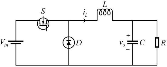
Figure 1.
Topology of DC-DC buck converter.
The conventional model of a buck converter commonly defines the output voltage vo as the state variable to conveniently reveal the dynamic characteristics of the system output voltage. However, in practical applications, the main objective of the control system is to make the actual output voltage track the reference voltage as accurately as possible. The tracking error model, by explicitly introducing the output error as a state variable, provides an intuitive representation of the deviation between the system output voltage and the reference voltage. Therefore, the tracking error model can be derived by defining the system state variable x1 as the error between the output voltage vo and the reference voltage vr, which simplifies the representation of performance indices in the state-space domain. This allows the controller to be designed directly based on the tracking error, facilitating the computation of the optimal control law. In addition, the output tracking error state-space equation can be deduced as follows:
where the state variable , representing the rate of variation in the voltage error, can be defined as the derivative of x1. Then, the following state-space Equation (3) can be obtained by substituting (1) into (2):
where the derivative of the reference voltage vr is assumed to be zero to simplify the model and controller design, as vr is typically set to a constant value or adjusted in a piecewise manner under different operating conditions in practical DC-DC converter applications. There are inevitable errors between the input voltage and the load resistance with their nominal values in practical buck converters, since the tracking error state model can be further reformulated as follows:
where Vin0 and R0 are the nominal value of Vin and R, respectively. Total disturbances d, including parameter variations, input voltage fluctuation and external uncertainties, can be defined as [25]. The state-space equation can be further established as following by defining x1 as the error-based system output variable:
where . Based on continuous-time state-space Equation (5), the discrete-time state-space Equation (6) can be formulated using the forward Euler approximation equation as follows:
where , , , . Matrix Ad and Bdu are the state matrix and control input matrix, respectively. Matrix Bdd and Cd are the disturbance input matrix and output matrix, respectively. The matrix symbol I and time notation Ts represent unit matrix and sampling time, respectively. The forward Euler approximation equation can be shown as follows:
2.2. Prediction of the Buck Converter
To address the limitations of the discrete-time state-space model in representing system states and designing constraints within CCS-MPC, an augmented state-space model is further derived, as shown in Equation (8). The augmented state vector includes both the original state variables and additional output states to facilitate controller design [26].
where state vector satisfies . The system model matrices A, B, Bd and C can be defined as , , and , respectively. Since the optimal control quantity is recalculated every cycle, the disturbances d can be considered to exist only in the current cycle, i.e., . The prediction of the future state quantity is deduced as follows:
where and mean control sequence and gain of control quantities, respectively. The term means the states after N steps predicted from moment k. According to (9), the prediction output matrix Y, defined as , can be obtained as follows:
where the matrices F, Φ, and D can be defined as and , respectively.
3. Control Strategy Design and Analysis
3.1. Design and Convergence Analysis of Reduced-Order Extended State Observer
The discrete-time state-space equation can be extended as follows:
Based on Equation (11), ESO can be further designed as follows:
where l1, l2, l3 are the observer gains. The variables z1, z2, and z3 represent the estimates of x1, x2, and x3, respectively, obtained by ESO. In particular, an estimated value of the total disturbances is defined as the extended state variable z3. Additionally, the output voltage can be directly measured by sensors, so the convergence rate of observer can also be accelerated through reducing its order [27]. In (12), the output voltage x1 can be measured, so the RESO can be designed as following (13) by replacing z1 with x1:
where gains of ESO β1, β2 can be selected with β1 = 2ω, β2 = ω2. The term ω means the bandwidth of ESO [28]. The rate of convergence can be regulated with observer gain, since the convergence rate of ESO increases with large observer gain.
Assumption 1.
For the DC-DC buck converter system, the total disturbances d(t) can be supposed to be bounded and satisfy .
Lemma 1.
[19] Considering that a nonlinear system satisfies input-to-state stable (ISS), the state variable condition is satisfied with the input condition.
The tracking errors between the estimated state and actual states of system are defined as , , so their derivations can be obtained as follows:
The tracking error Equation (14) can be further reformulated as follows:
The characteristic polynomial of (15) can be obtained as follows:
where , . According to Lemma 1, in the event of the disturbance under discussion in this paper satisfying the conditions set forth in Assumption 1, the observer will be convergent.
3.2. Model Predictive Controller Design
The duty ratio of a buck converter is bounded between 0 and 1 in general, so the control quantity should be bounded as . The complete MPC formulation, which includes the cost function, control horizon, predicted outputs, and system constraints, is presented as follows:
where the matrix is the expected sequence. The term is the expected signal at time ki. The expected sequence is 0 sequence, because the system output is based on errors. The diagonal matrix is the weighting coefficients of the cost function. The coefficients and mean feedback factor and the unit matrix, respectively. The partial derivative of the cost function J in Equation (17) should be equal to 0, so the solution can be obtained as follows:
where corresponds to the state feedback control gain under the predictive control framework to ensure that the controller can take into account the current state of the system for more accurate control. The parameter corresponds to the feedback control gain associated with Δd(k). It is used to ensure that the system maintains good performance and achieves control objectives even in the presence of disturbances.
3.3. Triggering Condition of ET-MPC
The event-triggered mechanism is integrated into the RESO-MPC framework, with a flexible design for the event trigger condition. The estimated state error is defined as follows:
where and are the state vector and estimated state in the future, respectively. The current and the next sampling instants are denoted by ti and ti+1, respectively. Subsequently, to ensure that the control system is input-to-state stable (ISS), it is necessary that the estimated state error satisfies the inequality:
where α and γ are both class functions. The variables and denote the Euclidean norm of e(t) and x(t), respectively. Based on (20), it is convenient to judge the stability of the system with external input [22]. Considering that the value of u(t) ranges within [0, 1], Equation (20) is differentiated. Meanwhile, the discrete-time state-space model of the buck converter (6) is substituted to obtain as follows:
where . For a practical DC-DC buck converter system, the range of current and voltage is limited to a certain extent. In addition, the variation speed of the current and voltage is also limited within a certain range by passive components. Therefore, variables and as state-related quantities must have an upper bound. The upper bounds of and are defined as follows:
The upper bounds of and are substituted into inequality (21) as follows:
To prove (24) satisfy inequation (20), variable is defined as follows:
Then, the derivation of (25) can be obtained based on (21) as follows:
Considering that (18) will equal 0 when t = ti, Equation (22) can be further derived as follows:
Inequality (26) can be solved on the basis of (27) as follows:
where . Then, the following Equation (29) can be obtained by substituting Equation (27) into (28):
Then, tet = ti+1-ti is defined as a preset sampling time bounded by the control chip calculation, so Equation (29) can be simplified as follows:
It is apparent that Equation (30) can match the form of (20) properly to ensure ISS, so Equation (30) can be used as a guidance to design the trigger condition. In addition, the tunable coefficient η could be introduced into (30) to balance the quantity of switch actions and performance regulation. Then, (30) can be improved as follows:
In light of the aforementioned derivation and demonstration, it can be posited that the triggering condition required to enable MPC controller can be designed as follows:
Since the controller is designed in discrete time, can be easily obtained based on RESO as follows:
Meanwhile, the total disturbance d can be replaced by its estimated value z3 obtained from the RESO. Equation (33) is substituted into (32), so the triggering condition is expressed as follows:
The left-hand side quantifies the deviation between the predicted and actual state evolution, indicating the extent to which the system deviates from the expected trajectory. It serves as the criterion for determining whether a control update is required. In designing the triggering threshold, it can be observed that the disturbance variation Δd reaches its peak at the initial stage of operation, when the buck converter begins to track the reference voltage. Based on this worst-case scenario, we selected the maximum observed Δd and applied a 1.2× safety margin, resulting in a fixed (Δd)max used for the triggering condition. This ensures feasibility of the triggering mechanism under real operating conditions. So the right-hand side defines an adaptive threshold composed of control gains (e.g., Kd, Bd), the upper bound of disturbance variation (Δd)max, the design parameter η, and the triggering period tet. This threshold reflects the disturbance tolerance and computational capability of the system. In addition, although the triggering condition can ensure that the output converges to the reference value, it is still necessary to introduce the following condition as an additional safeguard, as detailed below:
where ΔUc and m1 are the output voltage ripple and the steady-state error adjustment factor, respectively. The increment Δu(k) denotes the control increment output by the MPC controller at the current moment. The parameter m2 denotes the control increment adjustment factor. The parameter m1 is used to regulate to cope with the existence of steady-state error or the need to relax the constraints, while m2 is used to balance the control dynamics with the use of steady-state characteristics and constraints.
Based on the above ideas, the control flow can be described in detail as the following steps:
- (1)
- Parameter initialization: sequence pointer k, state quantities x1 and x2, and total disturbance d.
- (2)
- The state quantities x1, x2 and the total perturbation d are obtained by sampling and partial processing (including RESO).
- (3)
- Substitute the state quantity x1 and the control increment Δu(k) left over from the previous cycle into (35). If Equation (35) is satisfied, continue to the next step; if not, skip to step 5.
- (4)
- Continue to use the control quantity u of the previous moment and update the pointer k = N, and skip to step 11.
- (5)
- Determine whether k is equal to N + 1. If it is satisfied, skip to step 7; if not, continue to the next step.
- (6)
- Substitute the state quantities x1 and x2 and the total disturbance d into (34). If (34) is satisfied, continue to the next step; if not, skip to step 9.
- (7)
- The sequence of optimal control increments ΔU is calculated by model predictive controller.
- (8)
- Replace the original control sequence with the newly calculated control sequence and set the sequence pointer k to 1. Then skip to step 10.
- (9)
- The optimal control increment sequence ΔU remains unchanged and the sequence pointer k is increased by 1.
- (10)
- The kth control increment of the control increment sequence ΔU is taken and added to the control quantity of the previous cycle to obtain the control quantity u of this cycle.
- (11)
- Processing the control quantity u as a duty cycle and applying it to the DC-DC buck converter.
- (12)
- Determine whether the system needs to end the work. If so, stop the work; if not, return to step 2 and wait for the next cycle to start.
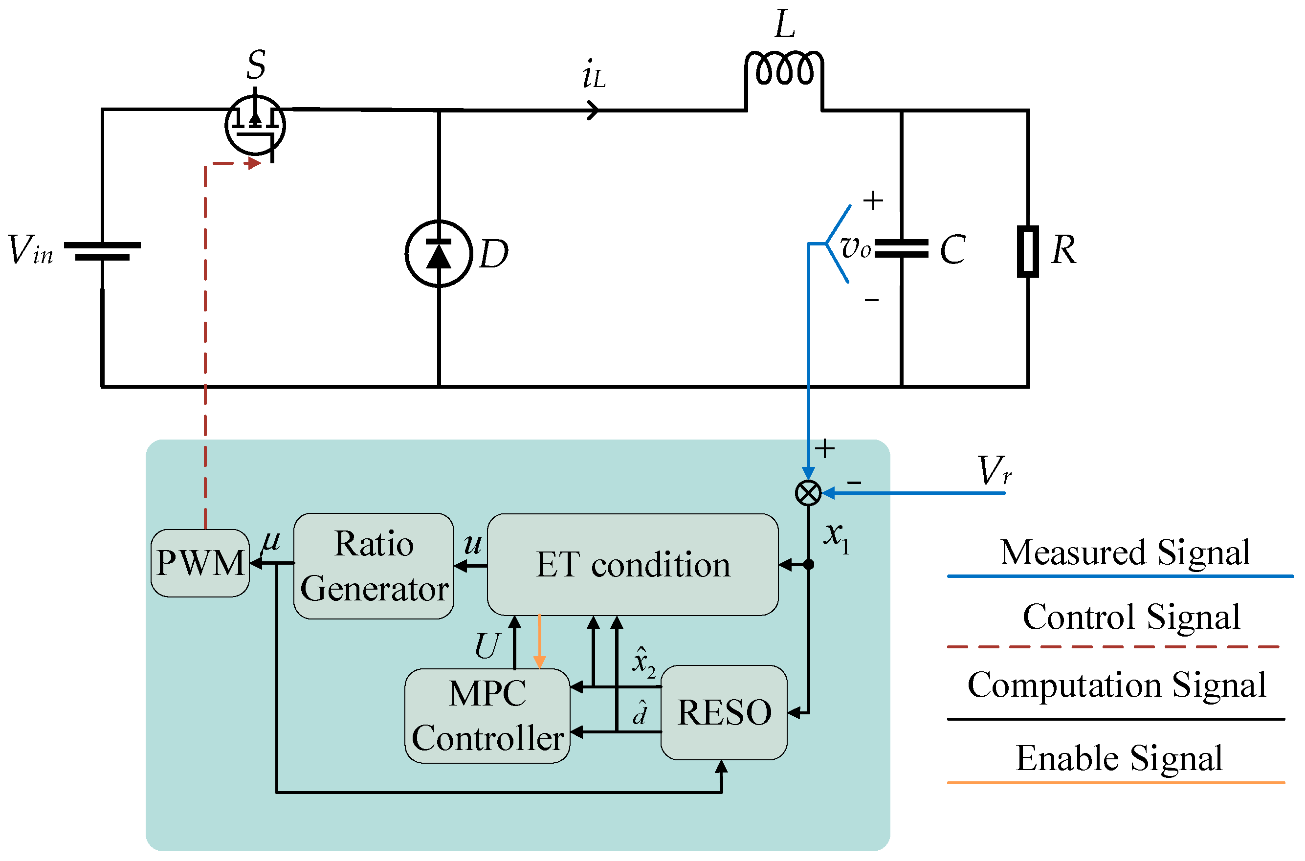
The structure of the proposed event-triggered-based model predictive control strategy for a DC-DC buck converter is illustrated in Figure 2, where the state x1 is directly given to RESO and the conditional trigger. In addition, the MPC controller can be designed by using the estimated values of RESO, i.e., and . Subsequently, the conditional trigger is calculated based on , and . It is then determined whether MPC should operate. The conditional trigger then determines the prevailing operational context on the basis of estimated states and disturbances. This ultimately determinates the actual control quantity u, which is either the previously established control quality u* or the quality derived from the revised control sequence U.
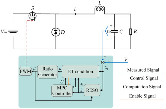
Figure 2.
The structure of the proposed ET-MPC scheme.
3.4. Stability Analysis of Closed-Loop System
Lemma 2.
[29] A closed-loop system controlled by an MPC controller is asymptotically stable if there exists a Lyapunov function V(x) satisfying the following conditions:
(1) V(x(k))≥ 0 for all x and V(0) = 0,
(2) ΔV(x) = V(x(k + 1)) − V(x(k)) < 0 for all x.
Equation (17) is substituted into (18) and simplified as follows:
where KMPC represents the state feedback control gain of the MPC controller. The coefficient Kd represents the feedback control gain related to Δd(ki). By substituting Equation (35) into (6), the closed-loop state-space representation of the system is derived as follows:
To analyze the stability of the closed-loop system, the Lyapunov function can be given as follows:
where and are the control and disturbance matrices of the closed-loop system, respectively. Assuming that the disturbance satisfies the conditions of Assumption 1, the inequality below can be established as follows:
Equation (40) can be further deduced as follows
Thus,
As a result, substituting the values of BMPC and Bd into the formula, Equation (42) shows that the closed-loop system (37) is asymptotically stable with respect to bounded Δd(k).
4. Experimental Verifications and Results Analysis
To evaluate the performance of the proposed ET-MPC scheme, comprehensive experimental comparisons are necessary. These comparisons aim to verify whether ET-MPC reduces computational complexity. At the same time, they assess whether it maintains better steady-state performance and stronger disturbance rejection compared to RESO-MPC.
4.1. Experimental Set-Up
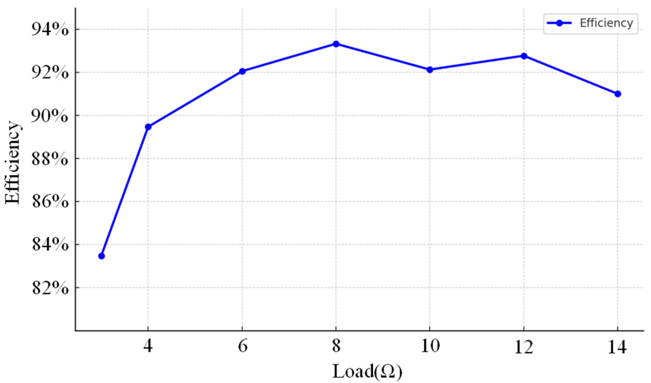
In order to assess the effectiveness of the proposed scheme in actual working conditions, the component parameters of the buck converter are detailed in Table 1. It was established that MOSFETs represented the optimal selection for switching devices, given their suitability for a range of potential applications involving high-frequency and low-power transmission [30]. In this study, the MOSFET model 15N10, manufactured by UMW (Shenzhen, China), is selected for the converter design based on its performance and compatibility with the system requirements. In this experimental setup, the power efficiency of the DC-DC converter can reach up to 93%. The efficiency under different loads is shown in Figure 3. In light of the aforementioned considerations, the experimental switching frequency was set to 50 kHz, while the control frequency was established at 500 Hz.

Table 1.
Parameters of buck converter component.
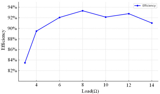
Figure 3.
Efficiency of buck converter.
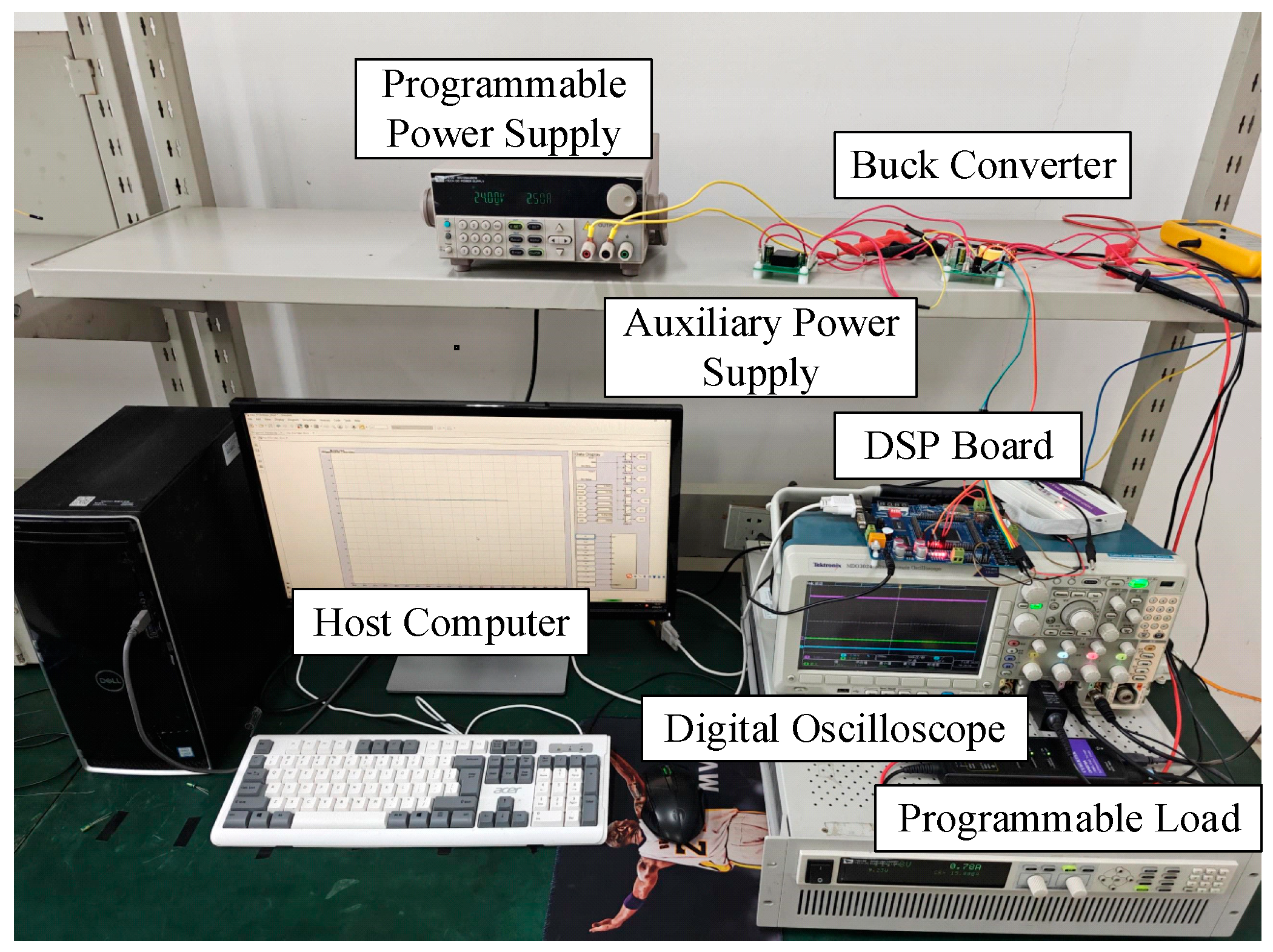
The designed control algorithm is implemented in PC MATLAB(2018b) using a graphical programming language, and the experimental platform is shown in Figure 4. A programmable DC power supply (model IT6722) and a programmable electronic load (model IT8816B), both manufactured by ITECH (New Taipei City, China), are used to provide the input voltage and to simulate varying load conditions, respectively. The input voltage, output voltage, and the trigger signal are observed using a digital oscilloscope. The first step is to automatically generate the control algorithm, then download it to the DSP28335 to complete the online simulation. The output voltage is acquired by the voltage sampling chip in the buck conversion circuit. Subsequently, the acquired voltage signal is transferred to the DSP, and the corresponding duty ratio is calculated by the MPC control algorithm. Ultimately, the PWM waveform will be generated by comparing the duty ratio with the sawtooth waveform to realize the tracking of the output voltage with the buck converter.
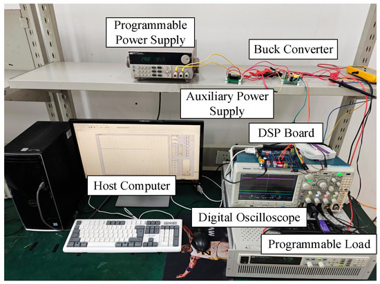
Figure 4.
Experimental test setup.
In order to encompass as many potential scenarios as possible, the experiments can be designed to include three distinct situations:
- (1)
- Variations in load equivalent resistance: The load equivalent resistance undergoes a sudden increase from 4 Ω to 8 Ω, followed by a precipitous decline to 3 Ω.
- (2)
- Variations in input voltage: The input voltage plummets from 24 V to 22 V at a rate of change of −21.67 V/s and surges from 22 V to 25 V at a rate of change of 18.75 V/s.
- (3)
- Variations in reference voltage: The reference voltage undergoes a step change from 12 V to 15 V, before returning to 12 V.
4.2. Experimental Results and Analyses
The experimental results are shown as Figure 5, Figure 6 and Figure 7. The result data are summarized in Table 2, where the amount of computation within 200 ms of the RESO-MPC scheme is selected for comparison with the ET-MPC scheme, since the RESO-MPC controller is always operating. In order to provide a more illustrative representation of the control scheme, the trigger signal is represented by a level signal. Upon the triggering of the MPC program, the trigger signal level will be pulled up; in the absence of such a triggering event, the level will be pulled down.

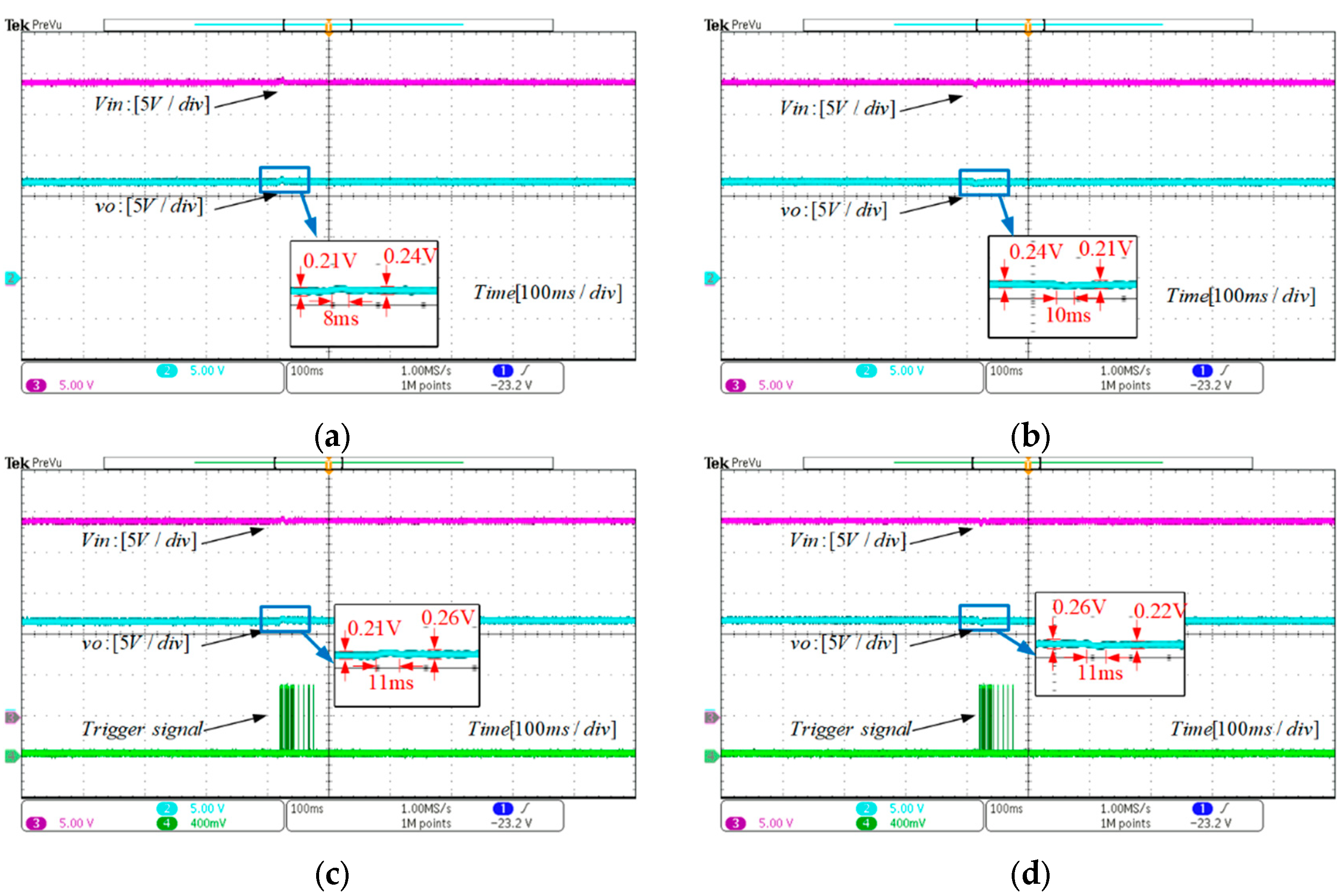
Figure 5.
Experimental transient-response evaluation with load equivalent resistance variations. (a) RESO-MPC with load rise; (b) RESO-MPC with load decline; (c) ET-MPC with load rise; (d) ET-MPC with load decline.
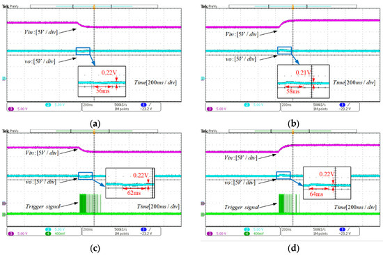
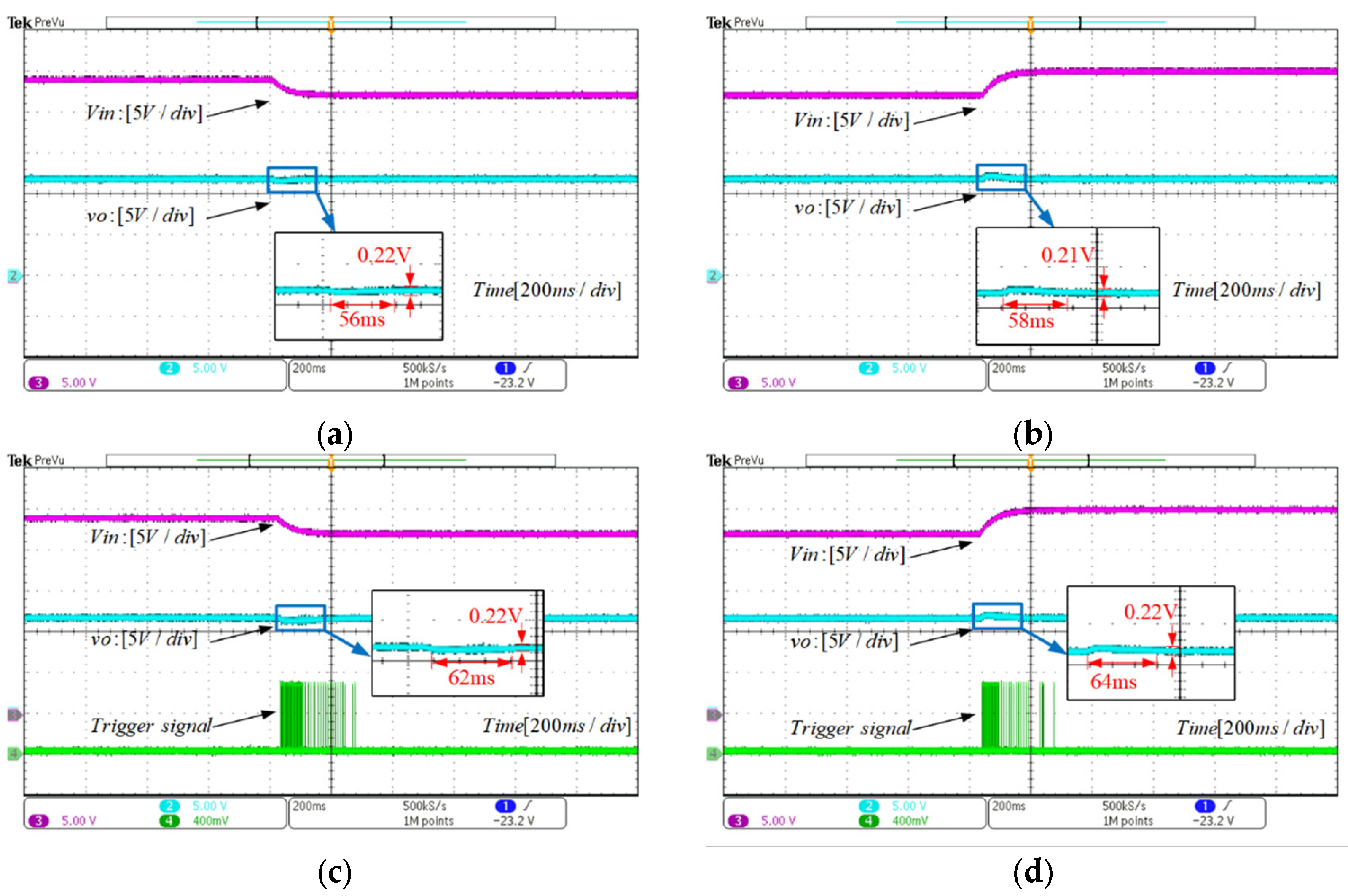
Figure 6.
Experimental transient-response evaluation with input voltage variations. (a) RESO-MPC with input decline; (b) RESO-MPC with input rise; (c) ET-MPC with input decline; (d) ET-MPC with input.
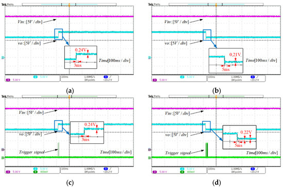
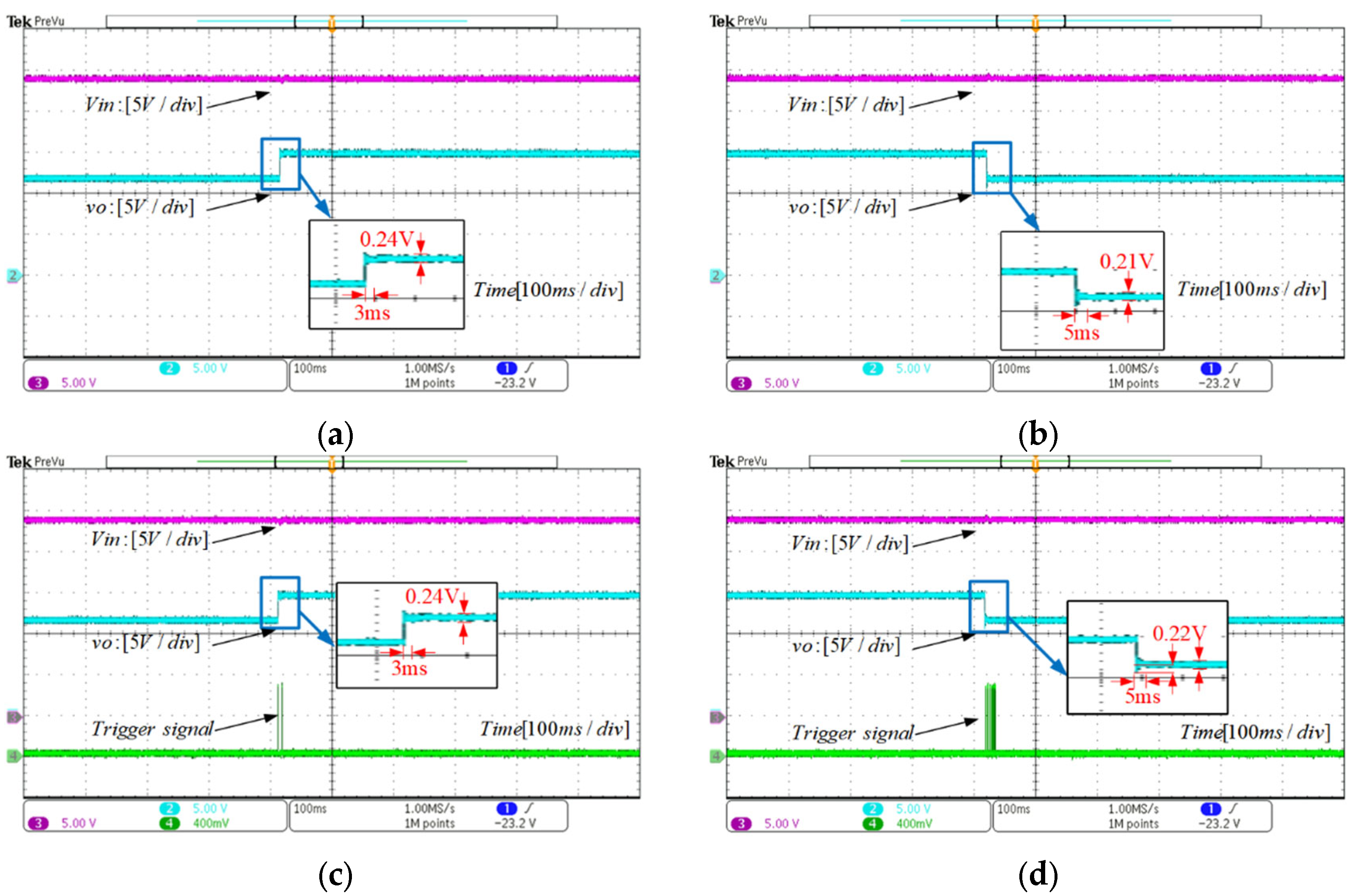
Figure 7.
Experimental transient-response evaluation with reference voltage variations. (a) RESO-MPC with reference rise; (b) RESO-MPC with reference decline; (c) ET-MPC with reference rise; (d) ET-MPC with reference decline.
Table 2.
Experimental results.
4.2.1. Experiment 1: Load Resistance Variations
RESO-MPC and ET-MPC strategies facing sudden load variations are demonstrated in Figure 5a–d. In Figure 5a, it can be seen that under light load conditions, the voltage ripple ΔvC corresponding to the RESO-MPC strategy is 0.21 V, which is 1.75% of the reference voltage. For the ET-MPC strategy, the voltage ripple ΔvC is also 0.21 V under light load conditions, but after the load is changed to 8Ω, the voltage ripple ΔvC of RESO-MPC is slightly better than ET-MPC. The response times of the two control strategies are also almost the same, with RESO-MPC only slightly better than ET-MPC. In addition, the voltage variation Δv of the RESO-MPC strategy due to the load step change is 0.12 V and 0.15 V in Figure 5a,b, respectively. However, the corresponding voltage variation Δv of ET-MPC is 0.13 V and 0.15 V in Figure 5c and Figure 5d, respectively.
4.2.2. Experiment 2: Input Voltage Variations
Figure 6a–d shows the two control strategies in the face of input voltage variations. Unlike the load variation, the input voltage variation leads to a slower response time, which is due to the fact that the change in the input is relatively slow and is not a mutation. However, interestingly, the output voltage under RESO-MPC and ET-MPC controllers only experiences slight fluctuations during input voltage variations because disturbance of the buck converter is compensated by RESO. In Figure 6a,b, the input voltage variations result in response times of 56 ms and 58 ms for the RESO-MPC. It is shown in Figure 6c,d that the response times of the proposed ET-MPC for input voltage variations are 62 ms and 64 ms, which are similar to the RESO-MPC.
4.2.3. Experiment 2: Reference Voltage Variations
Figure 7a–d shows the two control strategies facing the reference voltage variation. In Figure 7a, it can be seen that the voltage ripple ΔvC becomes 0.24 V, which is 1.6% of the reference voltage, after a sudden change of the reference voltage under the RESO-MPC strategy. The voltage ripple ΔvC after a sudden change of the reference voltage under the ET-MPC strategy is also 0.24 V, and the corresponding response times of the two control strategies are also almost the same. However, the static performance of the ET-MPC controller is not as good as that of the RESO-MPC controller, considering that it can lead to steady-state errors when the output error is less than a certain range and the control increment in the previous moment is less than a certain range or when the trigger condition is not reached either.
Above all, the incorporation of an event-triggering mechanism can mitigate the computational constraints associated with the MPC controller, while simultaneously enhancing the resilience of MPC through the integration of a tracking error model and RESO. Therefore, the ET-MPC configuration is particularly well-suited to applications where a single control chip is responsible for multiple controlled converters and is susceptible to external disturbances.
5. Conclusions
The objective of this study was to evaluate the performance of the MPC controller in terms of both steady-state operation and anti-disturbance capability, as well as to assess the computational reduction achieved by the MPC controller in the context of a DC-DC buck converter. A RESO-ERMPC controller has been designed with the objective of reducing the computational burden while maintaining the ability to restrain disturbances caused by variations in input voltage and load. Its effectiveness and efficiency have been validated through experiments compared with RESO-MPC.
The results of experiments indicate that: (1) The proposed ET-MPC controller has less computation than RESO-MPC and MPC. (2) Despite its computational reduction, the proposed controller retains a strong disturbance rejection capacity similar to that of the RESO-MPC controller.
Author Contributions
Methodology, K.C.; Validation, D.C.; Investigation, W.C.; Resources, J.L.; Writing—original draft, Z.Y.; Supervision, S.L. All authors have read and agreed to the published version of the manuscript.
Funding
This research received no external funding.
Data Availability Statement
The original contributions presented in this study are included in the article. Further inquiries can be directed to the corresponding author.
Conflicts of Interest
The authors declare no conflict of interest.
References
- Mohammed, D.M.; Hassan, R.F.; Yasin, N.M.; Alruwaili, M.; Ibrahim, M.A. A Comparative study of direct power control strategies for STATCOM using three-level and five-level diode-clamped inverters. Energies 2025, 18, 3582. [Google Scholar] [CrossRef]
- Zhou, S.; Zhou, G.; He, M.; Mao, S.; Zhao, H.; Liu, G. Stability effect of different modulation parameters in voltage-mode PWM control for CCM switching DC-DC converter. IEEE Trans. Transp. Electrif. 2024, 10, 2408–2422. [Google Scholar] [CrossRef]
- Shrivastava, A.; Calhoun, B.H. A DC–DC converter efficiency model for system level analysis in ultra low power applications. J. Low Power Electron. Appl. 2013, 3, 215–232. [Google Scholar] [CrossRef]
- Veerabathini, A.; Furth, P.M. High-Efficiency Switched-Capacitor DC-DC Converter with Three Decades of Load Current Range Using Adaptively-Biased PFM. J. Low Power Electron. Appl. 2020, 10, 5. [Google Scholar] [CrossRef]
- Garcés-Ruiz, A.; Riffo, S.; González-Castaño, C.; Restrepo, C. Model predictive control with stability guarantee for second-order DC/DC converters. IEEE Trans. Ind. Electron. 2024, 71, 5157–5165. [Google Scholar] [CrossRef]
- Wang, S.; Li, S.; Su, J.; Li, J.; Zhang, L. Extended state observer based nonsingular terminal sliding mode controller for a DC-DC buck converter with disturbances: Theoretical analysis and experimental verification. Int. J. Control 2023, 96, 1661–1671. [Google Scholar] [CrossRef]
- Liu, L.; Zheng, W.X.; Ding, S. An adaptive SOSM controller design by using a sliding-mode-based filter and its application to buck converter. IEEE Trans. Circuits Syst. I Regul. Pap. 2020, 67, 2409–2418. [Google Scholar] [CrossRef]
- Peng, Q.; Zhou, S.; Ma, F.; Huang, G.; Fan, R. A model predictive control of three-level cascaded noninverting buck–boost converter for energy storage system. IEEE Trans. Ind. Electron. 2025, 72, 4933–4942. [Google Scholar] [CrossRef]
- Wang, B.; Kanamarlapudi, V.R.K.; Xian, L.; Peng, X.; Tan, K.T.; So, P.L. Model predictive voltage control for single-inductor multiple-output DC–DC converter with reduced cross regulation. IEEE Trans. Ind. Electron. 2016, 63, 4187–4197. [Google Scholar] [CrossRef]
- Zhang, X.; Chen, R. An improved model predictive voltage control for PMSM drives without motor parameters. CES Trans. Electr. Mach. Syst. 2024, 8, 471–480. [Google Scholar] [CrossRef]
- Rosolia, U.; Guastella, D.C.; Muscato, G.; Borrelli, F. Model predictive control in partially observable multi-modal discrete environments. IEEE Control Syst. Lett. 2023, 7, 2161–2166. [Google Scholar] [CrossRef]
- Zhang, J.; Wang, S. Fractional-order linear active disturbance rejection control strategy for DC-DC BUCK converters. Electronics 2025, 14, 2226. [Google Scholar] [CrossRef]
- Kitaba, T. Modeling the system for hybrid renewable energy using highly efficient converters and generator. CES Trans. Electr. Mach. Syst. 2024, 8, 356–366. [Google Scholar] [CrossRef]
- Lu, H.; Li, J.; Li, S.; Wang, S.; Xiao, Y. Finite-time extended state observer enhanced nonsingular terminal sliding mode control for buck converters in the presence of disturbances: Design, analysis and experiments. Nonlinear Dyn. 2024, 112, 7113–7127. [Google Scholar] [CrossRef]
- Sun, J.; Xu, S.; Ding, S.; Pu, Z.; Yi, J. Adaptive conditional disturbance negation-based nonsmooth-integral control for PMSM drive system. IEEE/ASME Trans. Mechatron. 2024, 29, 3602–3613. [Google Scholar] [CrossRef]
- Zhang, Y.; Jin, J.; Huang, L. Model-free predictive current control of PMSM drives based on extended state observer using ultralocal model. IEEE Trans. Ind. Electron. 2021, 68, 993–1003. [Google Scholar] [CrossRef]
- Liu, X.; Qiu, L.; Wu, W.J.; Ma, J.; Fang, Y.T.; Peng, Z.H.; Wang, D.; Rodríguez, J. Event-triggered ESO-based robust MPC for power converters. IEEE Trans. Ind. Electron. 2023, 70, 2144–2152. [Google Scholar] [CrossRef]
- Sun, C.; Wang, R.; Sun, Q.; Zhang, H. A novel synchronous rectification scheme with low computational burden for LLC resonant converter in EV charger applications. IEEE Trans. Ind. Electron. 2023, 70, 8991–9003. [Google Scholar] [CrossRef]
- Wang, J.; Rong, J.; Yu, L. Reduced-order extended state observer based event-triggered sliding mode control for DC–DC buck converter system with parameter perturbation. Asian J. Control 2021, 23, 1591–1601. [Google Scholar] [CrossRef]
- Peng, C.; Li, F. A survey on recent advances in event-triggered communication and control. Inf. Sci. 2018, 457, 113–125. [Google Scholar] [CrossRef]
- Wang, B.; Huang, J.; Wen, C.; Rodriguez, J.; Garcia, C.; Gooi, H.B.; Zeng, Z. Event-triggered model predictive control for power converters. IEEE Trans. Ind. Electron. 2021, 68, 715–720. [Google Scholar] [CrossRef]
- Tabuada, P. Event-triggered real-time scheduling of stabilizing control tasks. IEEE Trans. Autom. Control 2007, 52, 1680–1685. [Google Scholar] [CrossRef]
- Hu, Z.R.; Shi, P.; Wu, L.G. Polytopic event-triggered robust model predictive control for constrained linear systems. IEEE Trans. Circuits Syst. I Regul. Pap. 2021, 68, 2594–2603. [Google Scholar] [CrossRef]
- Qin, B.; Yan, H.; Zhang, H.; Wang, Y.; Yang, S.X. Enhanced reduced-order extended state observer for motion control of differential driven mobile robot. IEEE Trans. Cybern. 2023, 53, 1299–1310. [Google Scholar] [CrossRef]
- Li, S.Q.; Lu, H.; Li, J.; Zheng, T.; He, Y. Fractional-order sliding mode controller based on ESO for a buck converter with mismatched disturbances: Design and experiments. IEEE Trans. Ind. Electron. 2025, in press. [CrossRef]
- Wang, B.Z.; Li, S.Q.; Kan, S.Q.; Li, J. Enhanced tracking of DC-DC buck converter systems using reduced-order extended state observer-based model predictive control. Int. J. Intell. Syst. 2023, 2, 143–152. [Google Scholar] [CrossRef]
- Sun, Y.; Ma, S. Output regulation of switched singular systems based on extended state observer approach. Appl. Math. Comput. 2021, 399, 126020. [Google Scholar] [CrossRef]
- Ma, C.; Wang, J. Applicability analysis of extended state observer-based control for systems subject to parametric disturbances. ISA Trans. 2022, 130, 226–234. [Google Scholar] [CrossRef]
- Karami, Z.; Shafiee, Q.; Sahoo, S.; Yaribeygi, M.; Bevrani, H.; Dragicevic, T. Hybrid model predictive control of DC-DC boost converters with constant power load. IEEE Trans. Energy Convers. 2021, 36, 1347–1356. [Google Scholar] [CrossRef]
- Li, N.; Zhang, S.; Jiang, Y. Junction temperature estimation model of power MOSFET device based on photovoltaic power enhancer. J. Low Power Electron. Appl. 2025, 15, 17. [Google Scholar] [CrossRef]

Disclaimer/Publisher’s Note: The statements, opinions and data contained in all publications are solely those of the individual author(s) and contributor(s) and not of MDPI and/or the editor(s). MDPI and/or the editor(s) disclaim responsibility for any injury to people or property resulting from any ideas, methods, instructions or products referred to in the content. |
© 2025 by the authors. Licensee MDPI, Basel, Switzerland. This article is an open access article distributed under the terms and conditions of the Creative Commons Attribution (CC BY) license (https://creativecommons.org/licenses/by/4.0/).