Microstrip Line Modeling Taking into Account Dispersion Using a General-Purpose SPICE Simulator

Abstract

XSPICE models for a generic transmission line, a microstrip line, and coupled microstrips are presented. The developed models extend general-purpose circuit simulation tools using RF circuits design features. The models could be used for circuit simulation in frequency, DC, and time domains for any active or passive RF or microwave schematic (including microwave monolithic integrated circuits—MMICs) involving transmission lines. The presented models could be used with any circuit simulation backend supporting XSPICE extensions and could be integrated without patching the core simulator code. The presented XSPICE models for microstrip lines take into account the frequency dependency of characteristic impedance and dispersion. The models were designed using open-source circuit simulation software. This study provides a practical example of the low-noise RF amplifier (LNA) design with Ngspice simulation backend using the proposed models.

1. Introduction

Circuits with distributed parameters are essential components of electronic devices operating in the UHF band and above [1,2]. Examples include communication equipment, wireless network systems [3], radar systems, passive filters [4], RF energy harvesters [5], and more. Lumped inductance and capacitance devices cannot be implemented at these frequencies and cannot be used as the resonant system. At the millimeter waveband and above, the lumped device size may become comparable to that of the wavelength. The circuits with distributed parameters, including microstrip lines, provide a better performance. For example, the Q-factor of the spiral inductor is in the range of 20-50 [6], but for the microstrip line resonator, a Q-factor of 250 may be achieved [2].

The design of both active and passive RF and microwave devices and systems [7], including modern MMICs [8], involves the circuit simulation stage. Proprietary software such as AWR Microwave Office or Keysight ADS is often used for this purpose, offering advanced features for simulating schematics with transmission lines. Open microelectronics process design kits (PDKs) [9] have emerged in recent years. The IHP 130 nm BiCMOS OpenPDK [10] provides SiGe devices operating up to 300 GHz and can be used for RF IC design. The PDK developer recommends using Ngspice as the simulation kernel and Qucs-S as the schematic capture tool when proprietary simulators are unavailable. Several studies [11,12,13] highlight the growing demand for open PDKs in integrated circuit development.

The SPICE [14,15] simulation kernel is an industry standard for circuit simulation [16], with both proprietary and open-source implementations available. Electronic component vendors distribute simulation models as SPICE netlist files. However, most open-source and freeware SPICE-compatible tools lack RF simulation features. The SPICE standard supports two types of transmission line model: a lossless transmission line defined by length and wave impedance; a lossy transmission line defined by inductance (L), capacitance (C), and resistive losses (R or G) per meter; and a uniform distributed RC-line (URC). None of these models accurately represent microstrip lines due to their frequency-dependent parameters. Additionally, SPICE does not support frequency-dependent instance parameters or coupled transmission line models.

Several open-source solutions extend SPICE for RF circuit analysis:

• Qucsator is an open-source simulation backend that supports the simulation of microstrip lines and advanced RF features [17,18]. The main disadvantage of this simulator is its very poor SPICE compatibility. It uses an unique netlist syntax and supports only a limited subset of the SPICE model. This makes difficult to integrate Qucsator into open PDKs.
• Scikit-RF [19] is an extension package for the Python programming language. It enables the calculation of RF circuits using Python scripts and allows us to define the transmission line structure and more complex schematics. This tool does not allow us to import SPICE models.
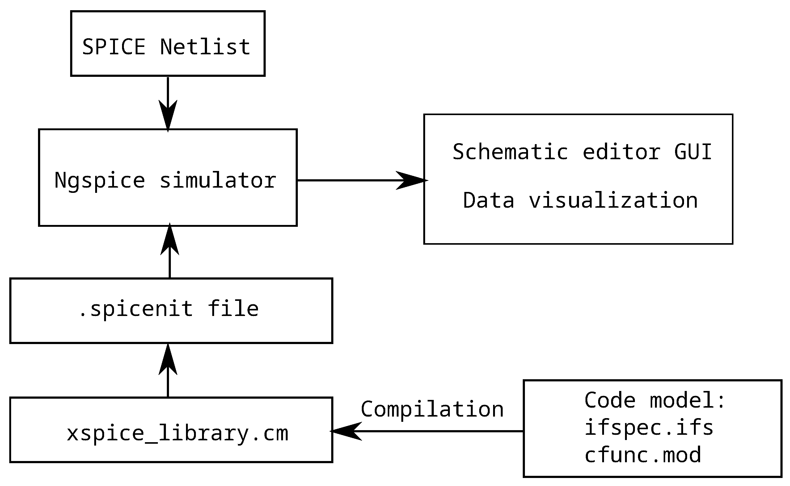
• The Ngspice [20] simulation backend introduces RF simulation features, including scattering matrix (S-parameter) analysis. Ngspice has good compatibility with SPICE models provided by electronic component vendors. This simulation backend may be used from Qucs-S [21] or KiCAD GUI. However, the transmission line models in Ngspice are represented only by lossy and lossless lines, as well as the URC line.

The underlying mathematics of transmission lines models in both proprietary and free simulators is based on works by Hammerstad [22] and Kirschning [23] et al. However, new methods of microstrip structure simulation involving SPICE-EM simulation have emerged in recent years [24,25]. The frequency of the microstrip structure is simulated with an electromagnetic (EM) simulator and then substituted into the SPICE kernel. While precise, this method is computationally intensive, creating a need for faster alternatives to estimate schematic characteristics before EM simulation.

Summarizing all the above, we can conclude that the development of models for SPICE kernels, which could be used in the OpenPDK RF IC design flow, is an important task. There are several ways to add a new model in a SPICE-compatible simulator. Patching the core simulator code should be avoided due to the architecture of modern circuit simulation software. The model should be distributed as a shared object. The recommended strategies are as follows:

• Using a parametrized subnetlist (macromodel) is the most obvious strategy [26]. This device representation method may have performance issues for complex models. The frequency dependency may be not allowed in subnetlist parameters for some SPICE backends because of netlist syntax restrictions.
• The Verilog-A [27] hardware description language (HDL) is the preferred method for adding a model for modern circuit simulators. Verilog-A allows researchers to compile model as a binary shared module and attach it to the simulator. Recompiling and patching the simulation backend itself is not required. Ngspice supports Verilog-A using the OpenVAF compiler [28]. However, Verilog-A cannot be used to the represent transmission line model. Verilog-A describes an electronics device as its current–voltage (IV) curve. In fact, this device is represented as a network of controlled current and voltage sources. This does not allow researchers to define a model in the frequency domain using the two-port circuit matrices, which is required for transmission line representation.
• XSPICE CodeModels [29,30] could be an alternative to Verilog-A models. The XSPICE models could be defined separately for the frequency and time domains. This allows researchers to define frequency-domain models as the impedance or admittance matrix of a two-port circuit. The disadvantage of XSPICE is that it requires researchers to have C programming language knowledge for model design.

Considering the mentioned three strategies, the XSPICE technique could be selected for implementing microstrip line models for the Ngspice simulation backend. This research will provide XSPICE models for both the generic transmission line and microstrip lines, including the coupled line. The novelty of this research is the extension of the simulation features of general-purpose SPICE software. Adding the possibility of microstrip structure simulation will allow us to estimate the RF circuit parameters in a straightforward workflow without needing to switch the simulation kernel and/or export the schematic for third-party RF analysis software for seamless use of the existing SPICE models.

The rest of this study is organized as as follows: Section 2 gives the equations used to design the XSPICE model. Section 3 describes the implementation of the XSPICE models using the equations from the previous section. Section 4 provides simulation results using the designed XSPICE models. Section 5 gives the conclusion and summary of the achieved results.

2. Model Equations

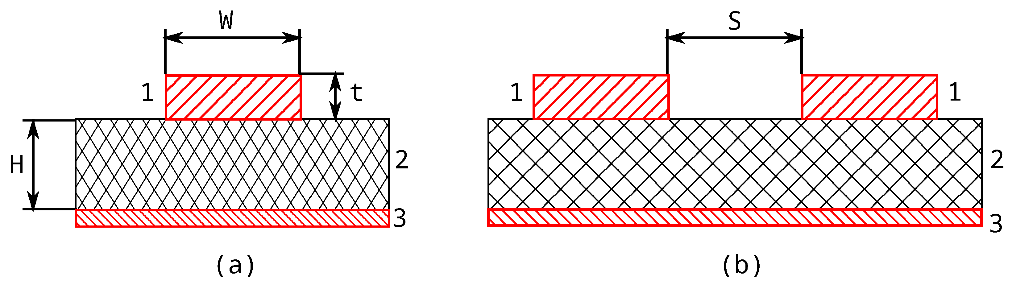
2.1. Microstrip Line and Coupled Microstrips

Microstrip lines consist of metal tracks on a dielectric substrate. The cross-section and dimensions of the microstrip structure are shown in Figure 1. L is the microstrip line length not shown in the figure.

Every transmission line could be characterized by its characteristic impedance $Z_L$. The characteristic impedance of the microstrip line depends not only on the line geometry and substrate properties but also on the frequency as follows: $Z_L=f(L,W,t,h,{\epsilon }_{r_{eff}},\omega )$. The effective relative dielectric permittivity of the substrate ${\epsilon }_{r_{eff}}$ also depends on the frequency. The equations for these dependencies are provided by Hammerstad [22] and Kirschning [23] and are not duplicated here.

The microstrip lines are a particular class of generic transmission lines defined by a known length and characteristic impedances and losses. The microstrip line and generic transmission line share the same equations for both the frequency and time domains. Thus, a model for the generic simple and coupled transmission lines will be considered in the next section. The main difference between the microstrip line model and the generic transmission line is that all components of the Z-parameter matrix depend on the operating frequency.

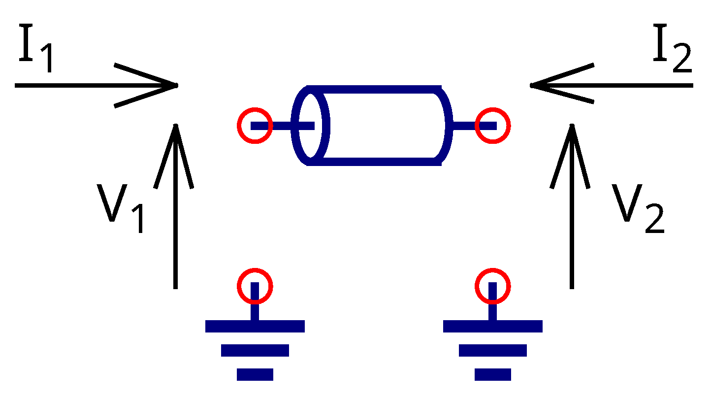
2.2. Generic Transmission Line

A transmission line is a passive electrical circuit with distributed parameters. Wave propagation in the transmission line can be described by the telegrapher equations [31]. Any transmission line can be represented as a two-port circuit, as shown in Figure 2, in which the arrows show the port voltage polarity and port current direction.

The currents and voltages (see Figure 2) at the line terminals can be expressed using the Z-parameter matrix. This form was selected because of some XSPICE restriction. The transient XSPICE model requires representing the circuit port as the current-controlled voltage source (CCVS, resistance type). This corresponds to the Z-matrix in the frequency domain. The port voltages and currents could be determined as follows:

$$\left[\begin{array}{c}{V}_1\\ V_2\end{array}\right]=\left[\begin{array}{cc}{Z}_{11}& Z_{12}\\ Z_{21}& Z_{22}\end{array}\right]·\left[\begin{array}{c}{I}_1\\ I_2\end{array}\right]$$

(1)

$Z_{11}=Z_{22}$ and $Z_{12}=Z_{21}$ because the transmission line is passive and t it is a symmetrical device. Therefore, only two parameters are required to describe the transmission line in the frequency domain. The expression for the Z-parameter can be found using the telegrapher equations solution:

$$Z_{11}={\displaystyle \frac{Z_L}{tanh\gamma L}}$$

(2)

$$Z_{12}={\displaystyle \frac{Z_L}{sinh\gamma L}}$$

(3)

where L is the transmission line length, $Z_L$ is the line characteristic impedance, and $\gamma =\alpha +j\beta$ is the propagation constant. $\alpha$ is the attenuation factor related to the losses in the line conductor and dielectric and $\beta$ is the imaginary part of the propagation constant. It is expressed as follows:

$$\beta =\sqrt{{\epsilon }_{r_{eff}}}\omega /C_0$$

(4)

where $C_0$ is the electromagnetic wave propagation speed in the vacuum and ${\epsilon }_{r_{eff}}$ is the effective relative dielectric permittivity for the propagation media. ${\epsilon }_{r_{eff}}$ may be frequency-dependent. Examples of frequency dependency can be found at [32,33].

The transients in the transmission line can be evaluated from the telegrapher equation solutions in the time domain. The time dependency of the voltages at the line ends is as follows:

$$V_1\left(t\right)=Z_L{I}_1\left(t\right)+A(Z_L{I}_2(t-\tau )+V_2(t-\tau ))$$

(5)

$$V_2\left(t\right)=Z_L{I}_2\left(t\right)+A(Z_L{I}_1(t-\tau )+V_1(t-\tau ))$$

(6)

where $\tau$ is the line propagation delay time:

$$\tau =L/C_0$$

(7)

This equation system simplifies for DC operation as follows:

$$V_1=V_2+Z_L{I}_2$$

(8)

$$V_2=V_1+Z_L{I}_1$$

(9)

According to these equations, the transmission for the DC and time domain can be represented as the equivalent circuit containing two resistors and two current-controlled voltage sources (CCVSs), as shown in Figure 3. The voltage sources V1 and V2 represent Equations (5) and (6).

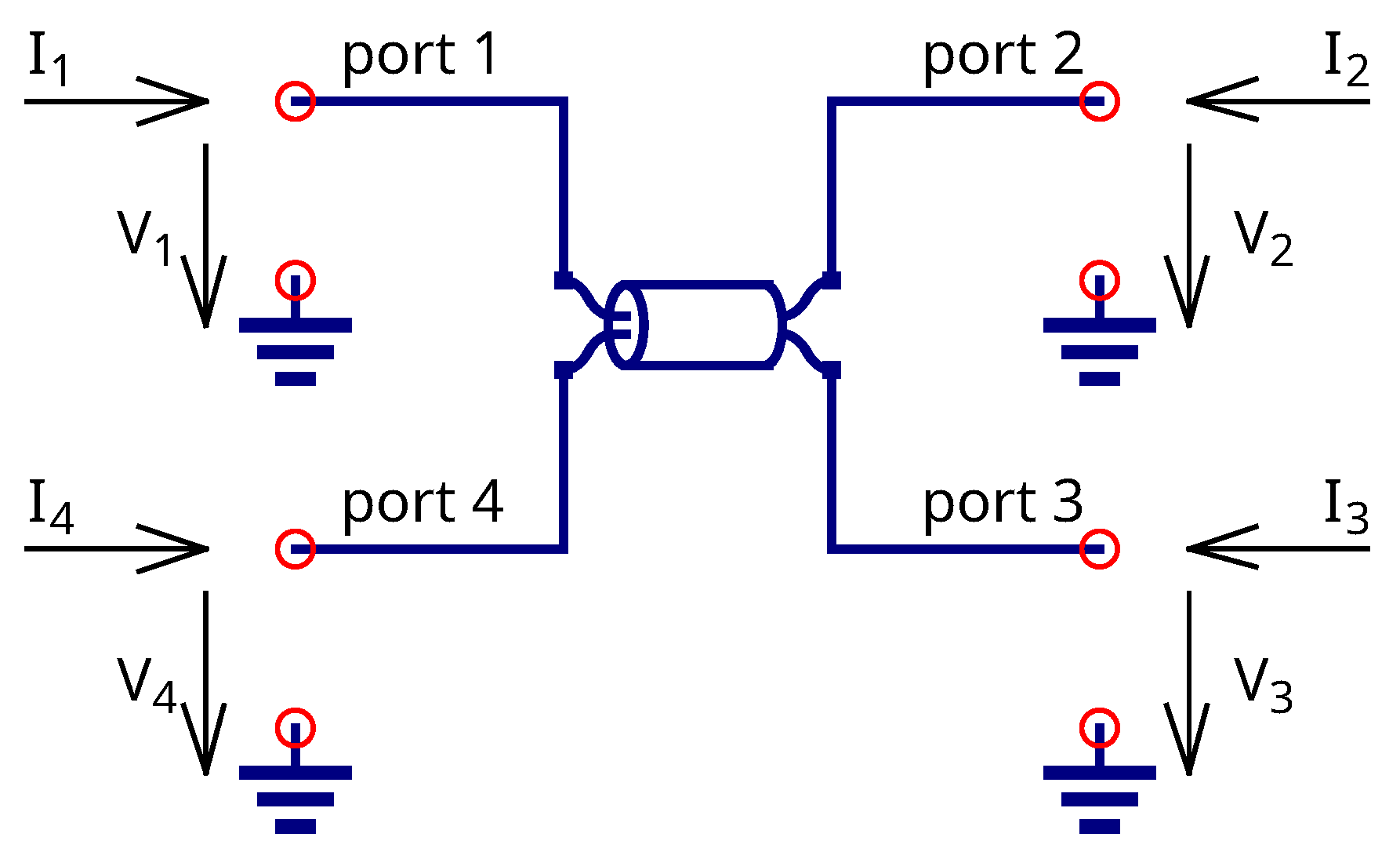
2.3. Generic Coupled Transmission Lines

Two generic coupled transmission lines can be represented as the four-port circuit (Figure 4).

According to the solution of the telegrapher equations, two wave modes travel in the coupled lines: even mode and odd mode. They are denoted by $Z_e$ (the characteristic line impedance for even mode) and by $Z_o$ (the same for odd mode). The Z-parameter matrix of the coupled lines for the frequency domain has a 4 × 4 dimension. Only four elements need to be evaluated because the device is symmetric and passive:

$$Z_{11}=Z_{22}=Z_{33}=Z_{44}={\displaystyle \frac{Z_o}{2tanh\left({\gamma }_{o}L\right)}}+{\displaystyle \frac{Z_e}{2tanh\left({\gamma }_{e}L\right)}}$$

(10)

$$Z_{12}=Z_{21}=Z_{34}=Z_{43}={\displaystyle \frac{Z_o}{2sinh\left({\gamma }_{o}L\right)}}+{\displaystyle \frac{Z_e}{2sinh\left({\gamma }_{e}L\right)}}$$

(11)

$$Z_{13}=Z_{31}=Z_{24}=Z_{42}={\displaystyle \frac{Z_e}{2sinh\left({\gamma }_{e}L\right)}}-{\displaystyle \frac{Z_o}{2sinh\left({\gamma }_{o}L\right)}}$$

(12)

$$Z_{14}=Z_{41}=Z_{23}=Z_{32}={\displaystyle \frac{Z_e}{2tanh\left({\gamma }_{e}L\right)}}-{\displaystyle \frac{Z_o}{2tanh\left({\gamma }_{o}L\right)}}$$

(13)

${\gamma }_e$ and ${\gamma }_o$ are the propagation constants for even mode and odd mode, respectively:

$${\gamma }_e={\alpha }_e+j\omega \sqrt{{\epsilon }_{r{e}_{eff}}}/C_0$$

(14)

$${\gamma }_o={\alpha }_o+j\omega \sqrt{{\epsilon }_{r{o}_{eff}}}/C_0$$

(15)

where ${\alpha }_e$ and ${\alpha }_e$ are the attenuation factor for even mode and odd mode. ${\epsilon }_{r{e}_{eff}}$ and ${\epsilon }_{r{o}_{eff}}$ are the relative dielectric permittivity values for even mode and odd mode, respectively.

The transient equations can be obtained from the solution of the telegrapher equation in the time domain. For convenience, let ports 1 and 3 be the input side of the coupled lines and ports 2 and 4 be the output side of the line (Figure 4). Thus, the even mode input current $J_{1e}$ can be determined via the following expression:

$$J_{1e}=(I_1+I_4)/2$$

(16)

The odd mode input current $J_{1o}$ can be determined as the input side port current difference as follows:

$$J_{1o}=(I_1-I_4)/2$$

(17)

The same is valid for the opposite side of the line (ports 2 and 3). The even mode output current $J_{2e}$ and odd mode input current $J_{2o}$ can be defined as follows:

$$J_{2e}=(I_2+I_3)/2$$

(18)

$$J_{2o}=(I_2-I_3)/2$$

(19)

The even mode input voltage $V_{1e}$, odd mode input voltage $V_{1o}$, even mode output voltage $V_{2e}$, and odd mode output voltage $V_{2o}$ can be defined as follows:

$$V_{1e}=(V_1+V_4)/2$$

(20)

$$V_{1o}=(V_1-V_4)/2$$

(21)

$$V_{2e}=(V_2+V_3)/2$$

(22)

$$V_{2o}=(V_2-V_3)/2$$

(23)

The next four equations determine the time dependencies of the odd and even mode voltages at the opposite sides of the line:

$$V_{1e}=Z_e{J}_{1e}+V_{2e}(t-\tau )+Z_e{J}_{2e}(t-\tau )$$

(24)

$$V_{1o}=Z_o{J}_{1o}+V_{2o}(t-\tau )+Z_o{J}_{2o}(t-\tau )$$

(25)

$$V_{2e}=Z_e{J}_{2e}+V_{1e}(t-\tau )+Z_e{J}_{1e}(t-\tau )$$

(26)

$$V_{2o}=Z_o{J}_{2o}+V_{1o}(t-\tau )+Z_o{J}_{1o}(t-\tau )$$

(27)

The port voltages can be expressed back from those determined above for the odd and even mode voltages:

$$V_1=V_{1o}+V_{1e}$$

(28)

$$V_2=V_{2o}+V_{2e}$$

(29)

$$V_3=V_{2e}-V_{2o}$$

(30)

$$V_4=V_{1e}-V_{1o}$$

(31)

Using Equations (24)–(27) and (28)–(31), it follows that the coupled transmission line can be represented in the DC and time domain as the equivalent circuit containing four CCVSs and four resistors.

3. XSPICE Model Generation

3.1. Common XSPICE Model Structure

Unlike Verilog-A models, which are distributed as a single file, XSPICE CodeModels consist of two files:

1.

ifspec.ifs, which contains the model interface description, i.e., port and parameter descriptions, including allowed boundaries.

2.

cfunc.mod, which contains model source code and internal logic. Here, we place one or more equations that describe component static current–voltage curves and other non-linear dynamic properties.

The *.ifs and*.mod files are known collectively as an XSPICE CodeModel. They are translated with an XSPICE preprocessor (CMPP) into a C code block ready for compilation and dynamic linking to form a model library file (*cm). In fact, a CodeModel uses the C programming language with macros and provides full access to C features.

The Qucs-S [34,35,36] open-source circuit simulation tool provides a unified GUI for open-source SPICE-compatible simulation backends and supports XSPICE model integration at the GUI level.

The data flow diagram (Figure 5) shows the interaction between the tools. The pairs of IFS and MOD files are processed with the preprocessor and C compiler to obtain the CM library. In fact, the CM library is the binary shared module with a specific interface. The CM libraries are specified in the spiceinit configuration file of the simulator and loaded at the execution time.

An N-port XSPICE device may be defined by port current equations ($I_1\dots I_N$) or voltage equations ($V_1\dots V_N$). The first approach is the voltage-controlled current source (VCCS), and the second approach is the current-controlled voltage source (VCCS).

Individual port currents or voltages may depend on other port currents or voltages. For the CCVS, we have the following:

$$\begin{array}{ccc}& V_1=f_1(I_1,\dots ,I_N)& \\ & \dots & \end{array}$$

(32)

$$\begin{array}{cc}& V_N=f_N(I_1,\dots ,I_N)\end{array}$$

(33)

An XSPICE device model is described by a gain matrix $\left(G_{AC}\right)$ in the AC domain, where $G_{ij}$ represents the i-th port to j-th port gain. For CCVS, this matrix is equal to the Z-parameter matrix, and VCCS, the gain matrix is equal to the Y-parameter matrix. The AC gain matrix of the N-port XSPICE device has the dimension $N\times N$.

The computation efficiency of the XSPICE model is comparable to those of the native models implemented in the simulator core level.

Table 1. Model simulation speed benchmark.

	Core Model	XSPICE	Verilog-A
Time (s)	0.143	0.156	2.58

shows the performance benchmarks for different models. The ideal capacitor model was implemented using XSPICE and Verilog-A and compared to the core model. The transient simulation of an RC-circuit response with 100,000 simulation points was used as the benchmark. Ngspice was operated on Linux platform using Core i7 CPU. The simulator execution time is provided in the table.

As can be seen, the simulation speed for XSPICE is around 15% less than that for the core model. The Verilog-A model is significantly slower. We can conclude from the presented results that the simulation performance loss using XSPICE models is acceptable.

3.2. Transmission Line Models Structure

The CCVS XSPICE model is preferable for representing the transmission line, because the transient equations are the voltage on the current dependencies. The port voltages also depend on delayed opposite-port voltages. while the XSPICE model has a restriction that allows us to find only the voltage or current input, but not both. Therefore, the two-port CCVS device requires two additional voltage-sensing ports. The common port connection of the XSPICE transmission line model is shown in Figure 6.

The pair of $V1+$ and $V1-$ pins represent the V1 port output, and the pair of pins $V1s+$ and $V1s-$ represent the port-sensing pins. The same is true for the opposite port $V2$. This circuit could be expanded for four-port devices such as the coupled lines.

The structure of the XSPICE model (the cfunc.mod file contents) can be expressed using the following pseudocode (shown in Listing 1):

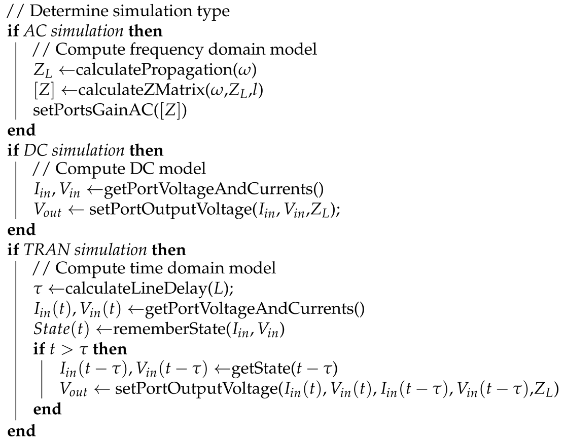
Listing 1. The pseudocode of the transmission line XSPICE model.

The algorithm of AC and DC modeling is straightforward. It needs to compute the AC gain matrix or the output port voltage $V_{out}$. The elements of the AC gain matrix are dependent on the line characteristic impedance $Z_L$ and line parameters. The characteristic impedance of the microstrip line depends on the frequency $\omega$ and should be evaluated before computing the AC gain matrix.

Simulating the line transients requires some preparation. The voltages and currents at input ports should be remembered for every time step in some data structures. At time $t>\tau$, the output voltages of the port are calculated according Equations (5) and (6). The voltage and current for the time point $t-\tau$ can be retrieved from the saved state. The line model must save at least $\tau /\Delta t$ previous simulation points, where $\Delta t$ is the simulation time step.

The coupled lines can be modeled with a similar approach, using equations from Section 2.3. The model should be expanded to include four ports. The microstrip line requires the same approach. The difference is that the line characteristic impedance is not retrieved from the model parameters. It should be evaluated as the function of the line geometry and frequency before computing the Z-matrix.

The parameters of the XSPICE models are summarized in

Table 2. Generic transmission line model parameters.

Model Parameter	Default Value	Unit	Description
$Z_L$	50.0	Ohm	line impedance
A	0	dB	line attenuation
L	1.0	m	line length
$Z_e$	50.0	Ohm	even mode impedance
$Z_o$	50.0	Ohm	odd mode impedance
$A_e$	0	dB	even mode attenuation
$A_o$	0	dB	odd mode attenuation
$E_{re}$	1.0		even mode relative dielectric permittivity
$E_{ro}$	1.0		odd mode relative dielectric permittivity
L	1.0	m	Line length

.

Microstrip lines require the dimensions (Figure 1) to be input instead of the characteristic impedance and attenuation. The substrate parameters are common for all microstrip models and provided in

Table 3. Common substrate parameters for microstrip line models.

Model Parameter	Default Value	Unit	Description
$e_r$	4.5		Relative dielectric permittivity
h	${10}^{-3}$	m	Substrate dielectric thickness
t	$35·{10}^{-6}$	m	Substrate conductor thickness
$\rho$	$2·{10}^{-8}$	Ohm · m	Substrate conductor resistance
$tand$	0		Dielectric loss tangent
D	0		RMS substrate roughness

. The substrate geometry is shown in Figure 1. The characteristic impedance and loss calculations are based on these data.

The SPICE netlist entry for the XSPICE microstrip model is shown in Listing 2. The microstrip line instance connection reflects Figure 6. The line dimensions and substrate parameters are defined by modelcard (follows after .MODEL keyword). The coupled microstrips are defined in a similar way, but the instance has four ports.

Listing 2. The implementation of the transmission line XSPICE model.

* Microstrip line instance A_MS1 %hd(p1 0) %hd(p2 0) %vd(p1 0) %vd(p2 0) MODEL_MS1 * Microstrip modelcard .MODEL MODEL_MS1 MLIN(l=100E-3 w=1E-3 model=0 disp=0 + er=4.5  h=1.55E-3  t=35u  tand=0.0167  rho=1.7E-8  d=0.15E-6 ) * Coupled microstrips instance A_MS2 %hd(p1 0) %hd(p2 0) %hd(p3 0) %hd(p4 0) + %vd(p1 0) %vd(p2 0) %vd(p3 0) %vd(p4 0) MODEL_MS2 * Coupled microstrip modelcard .MODEL MODEL_MS2 CPMLIN(L=20e-3 W=1e-3 S=0.3e-3 model=0 disp=0 + er=4.5  h=1.55E-3  t=35u  tand=0.0167  rho=1.7E-8  d=0.15E-6 )

4. Simulation Results

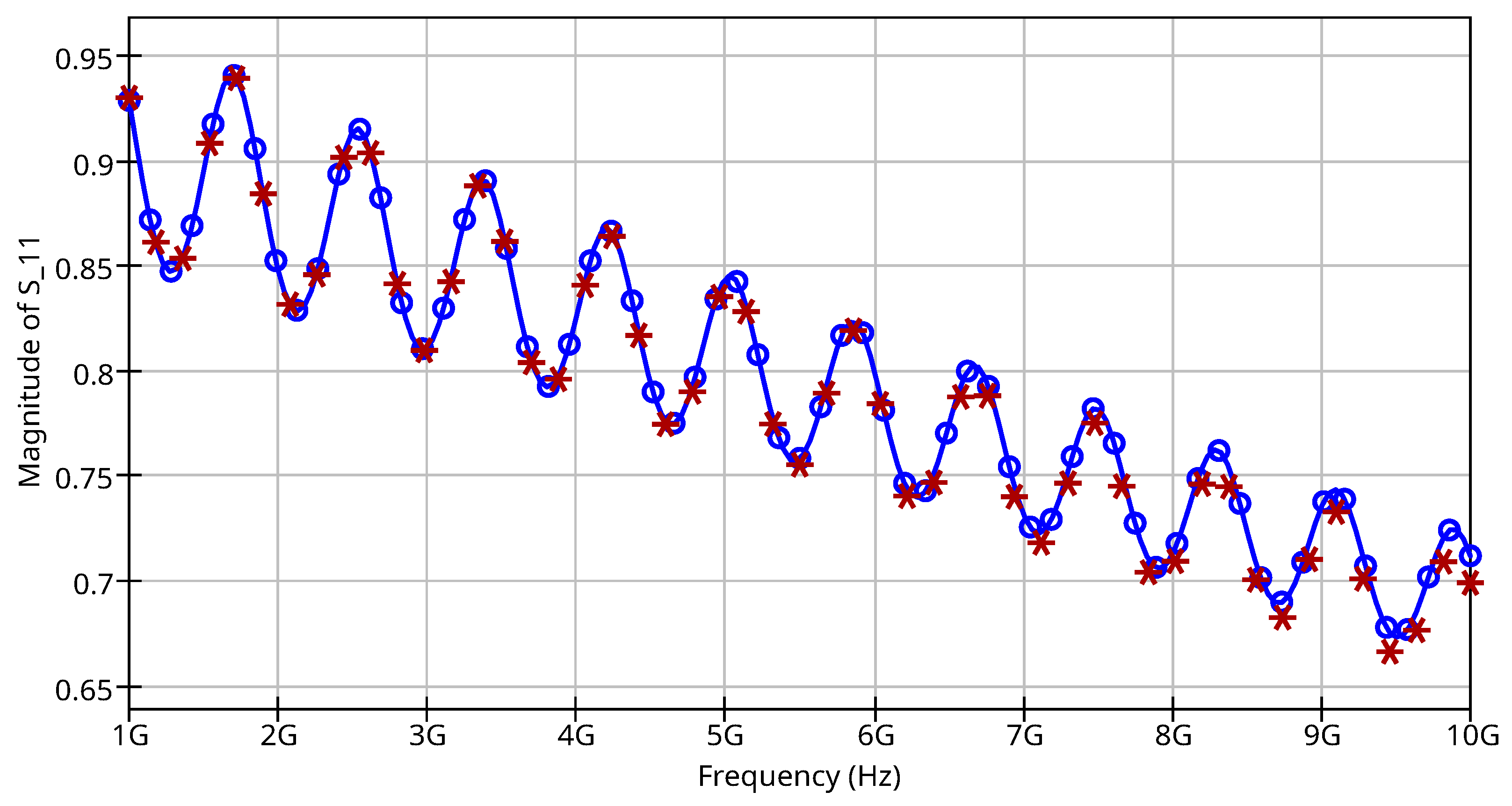
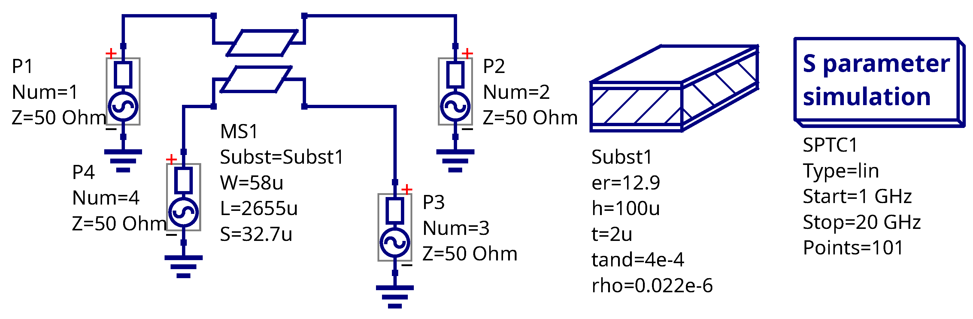
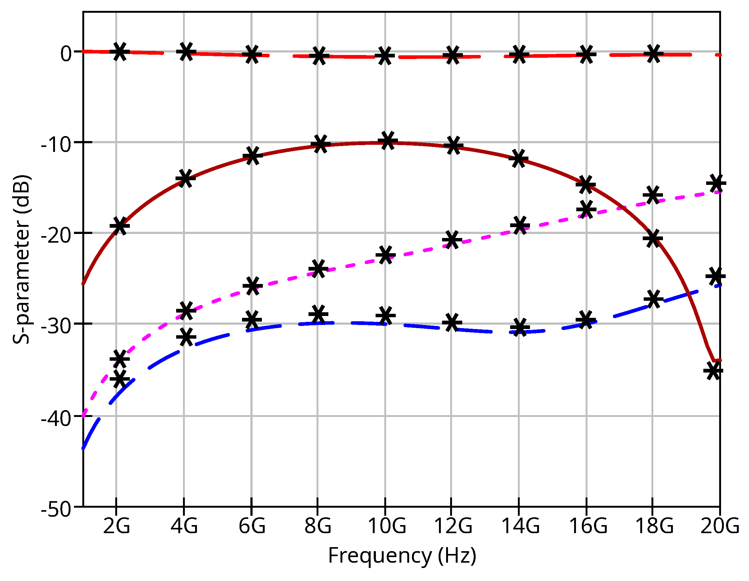
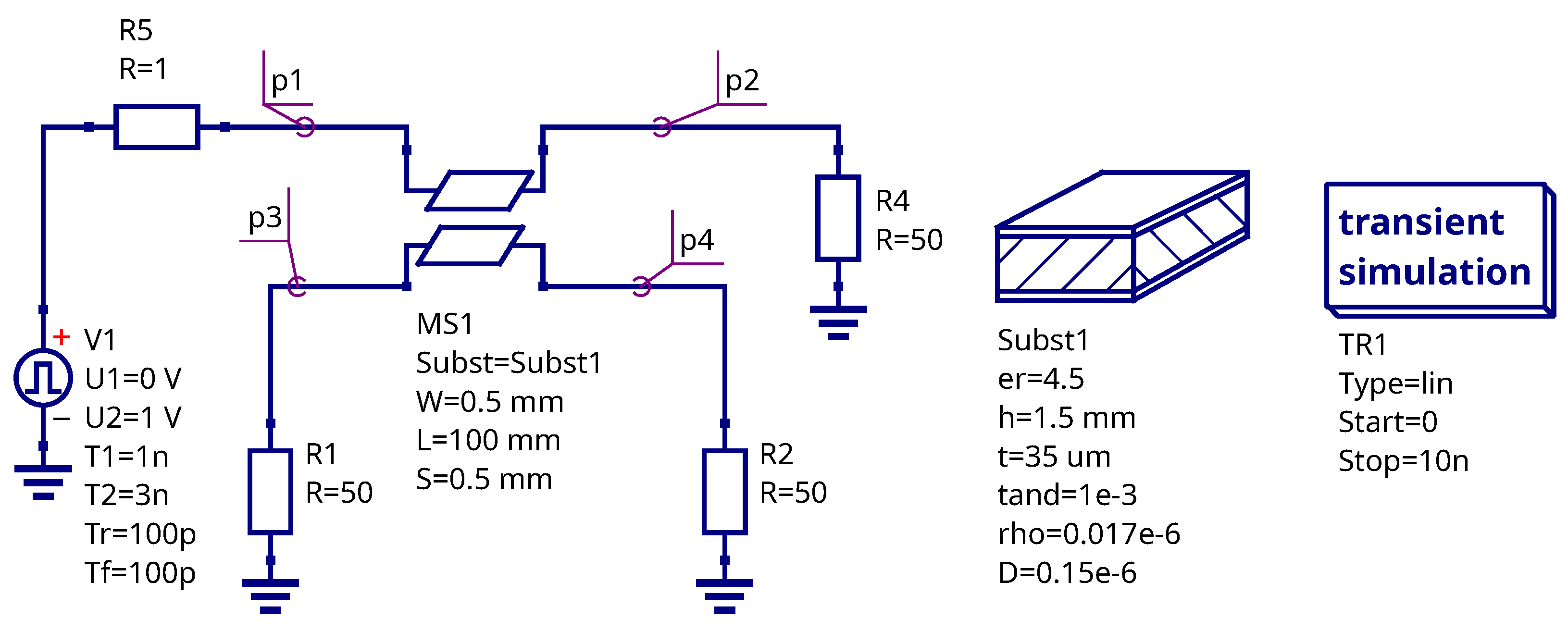
4.1. XSPICE Model Verification

The testbench circuit for the XSPICE model verification of the microstrip line is shown in Figure 7. The Qucs-S circuit simulator is used for the schematic input and automatic Ngspice netlist generation. The testbench schematic performs two-port scattering matrix analysis of the straight microstrip line. The simulation is conducted in a frequency range from 1 GHz to 10 GHz. The substrate parameters represent the FR-4 material.

The simulation results for the $S_{11}$ reflection coefficient are shown in Figure 8 and those for the $S_{21}$ forward transfer coefficient in Figure 9. $S_{11}=S_{22}$ and $S_{21}=S_{12}$ because the circuit is passive and symmetric. The analytical microstrip line model implemented in the Scikit-RF package is used for result verification. The microstrip models of Scikit-RF are verified using the measurement data with vector network analysis (VNA) equipment. The Ngspice simulation is compared with Qucsator simulation data, because this backend uses the same equations for characteristic impedance and dispersion as the proposed XSPICE models. The ScikitRF models are used in ADS mode (complex dielectric permittivity).

The numeric estimation of the simulation precision is shown in

Table 4. The numeric difference between the XSPICE model and the analytical model.

Frequency (GHz)	${\mathit{S}}_{11}$ difference, ADS Mode (%)	${\mathit{S}}_{21}$ difference, ADS Mode (%)	${\mathit{S}}_{11}$ Difference, Qucs Mode (%)	${\mathit{S}}_{21}$ Difference, Qucs Mode (%)
1	0.03	0.14	0.01	0.11
5	1.29	0.3	0.01	0.13
10	3.7	1.7	0.01	0.14

, which shows the difference in the S-parameter calculation (both $S_{11}$ and $S_{21}$) between the analytical model (ScikitRF) and the XSPICE model. ScikitRF [19] provides two types of microstrip line models: Keysight ADS mode (complex dielectric permittivity) and Qucsator mode (real dielectric permittivity).

The results from the simulation and analytical models with real effective dielectric permittivity are almost identical. The difference between the XSPICE simulation and analytical model with complex effective dielectric permittivity increases with the increase in frequency, but it remains within satisfactory limits.

A testbench schematic for the coupled microstrips is shown in Figure 10. This schematic represents a microstrip coupler on the GaAs substrate. The GaAs substrate parameters are taken according to [37] for the ambient temperature 300K. Such a structure is common in MMIC design [38,39]. S-parameter simulation is performed for this structure.

The simulation result is shown in Figure 11. The proprietary AWR Microwave Office simulation software package is used for model verification. The computation algorithm of AWR is unknown, but it is verified via measurement and electromagnetic simulation. The XSPICE models match well match with the AWR models.

A testbench schematic for the transient simulation is shown in Figure 12. Typical use cases for the transient simulation in transmission lines are crosstalk analysis [40,41] in printed circuit boards (PCBs) and transmission line pulse testing [42]. The test circuit features two 100mm length printed wires on an FR-4 substrate. The first line is connected to a pulsed source (nodes p1 and p2) and the second line (nodes p3 and p4) is terminated by resistors.

The simulation result is shown in Figure 13. The pulse at the line output is distorted (red trace). We can observe a voltage pulse at the unconnected line (magenta and brown traces).

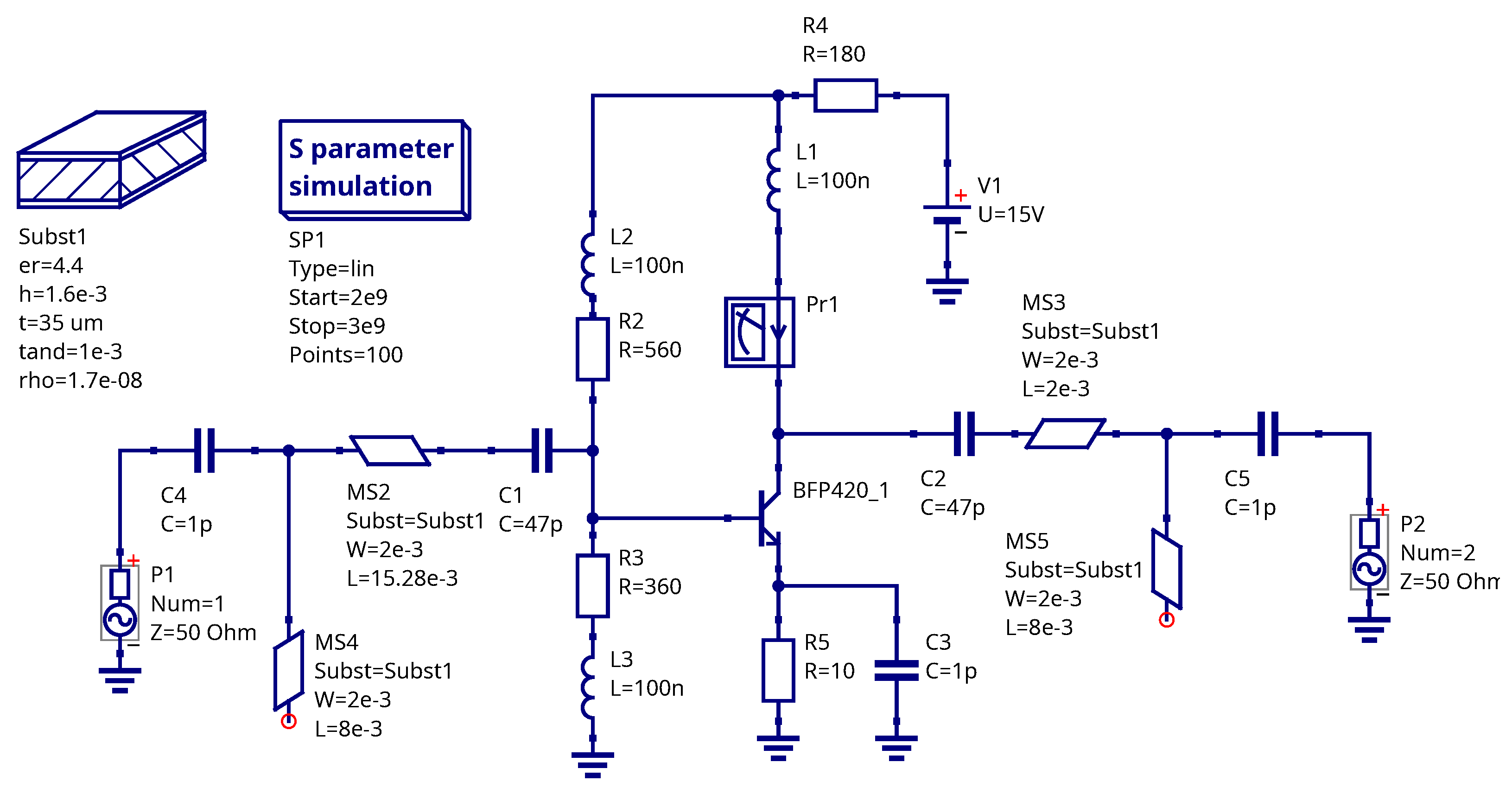
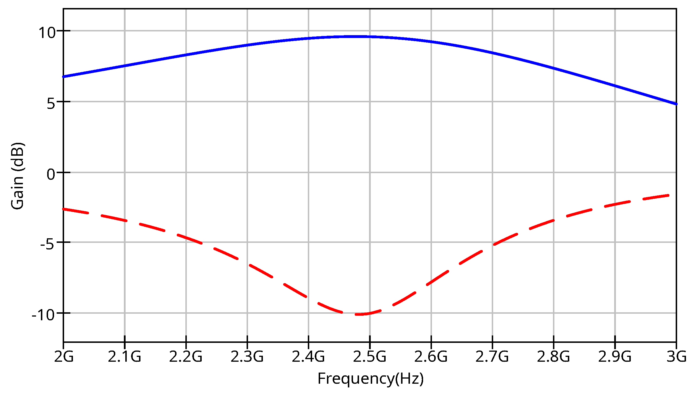
4.2. LNA Simulation Example

The LNA design provided by [43] is used as a reference. The report contains an amplifier design and simulation results using AWR software. This LNA operates in the 2.4 GHz band and uses a BFP420 bipolar transistor from Infineon. The schematic designed in Qucs-S is shown in Figure 14. Four microstrips (series stub and open end stub) are used to match the input and output of the amplifier. The substrate parameters are defined for FR-4 material with a 1.6 mm dielectric thickness and a 35 um copper thickness. The scattering matrix parameters are simulated in the frequency range of 2 GHz to 3 GHz.

The simulation results are shown in Figure 15. The gain ($S_{21}$) and return loss ($S_{11}$) match well with the data provided in [43].

5. Conclusions

The XSPICE models for microstrip and coupled microstrip lines developed in this research are compatible with any circuit simulation software supporting XSPICE extensions. These models can be seamlessly integrated into open-source microelectronic PDKs, enabling the analysis of RF electronic circuits in both the frequency and time domains. They provide accurate estimations of resonant properties, losses, and transients while accounting for different dispersion approximations.

The proposed microstrip lines models were tested with the Ngspice circuit simulation kernel and Qucs-S frontend. The simulation result matched well with those achieved by the analytical models provided by the Scikit-RF Python package (scikit-rf 1.8.0.) and proprietary RF simulation software (AWR) (V22.1). The structures of the XSPICE models overcame the limitations of Verilog-A by allowing the representation of devices described by Z- or Y-parameter matrices in the frequency domain. Additionally, the XSPICE models demonstrated satisfactory simulation performance (as shown in Table 1) and precision (Table 4).

While XSPICE enables model integration without modifying the core simulator code, it requires C programming knowledge for model development and debugging. This is a disadvantage compared to Verilog-A. Another limitation of the proposed models is the absence of an explicit noise definition.

The proposed XSPICE microstrip line models provide a new way to add other RF devices such as waveguides and more complex structures into SPICE simulation kernels. This advancement is particularly valuable for academic users and opens new possibilities for RF IC design using open PDKs and open-source circuit simulation tools, achieving results comparable to those of proprietary RF analysis software.

References

1. Vendelin, G.D.; Pavio, A.M.; Rohde, U.L.; Rudolph, M. Microwave Circuit Design Using Linear and Nonlinear Techniques; John Wiley & Sons: Hoboken, NJ, USA, 2021. [Google Scholar]
2. Harikirubha, S.; Baranidharan, V.; Saranya, S.; Keerthana, K.; Nandhini, M. Different shapes of microstrip line design using FR4 substrate materials—A comprehensive review. Mater. Today Proc. 2021, 45, 3404–3408. [Google Scholar] [CrossRef]
3. Shaban, M. Design and Modeling of a Reconfigurable Multiple Input, Multiple Output Antenna for 24 GHz Radar Sensors. Modelling 2025, 6, 2. [Google Scholar] [CrossRef]
4. Li, C.; Ma, Z.H.; Chen, J.X.; Wang, M.N.; Huang, J.M. Design of a Compact Ultra-Wideband Microstrip Bandpass Filter. Electronics 2023, 12, 1728. [Google Scholar] [CrossRef]
5. Colaiuda, D.; Ulisse, I.; Ferri, G. Rectifiers’ Design and Optimization for a Dual-Channel RF Energy Harvester. J. Low Power Electron. Appl. 2020, 10, 11. [Google Scholar] [CrossRef]
6. Pirouznia, P.; Ganji, B.A. Analytical optimization of high performance and high quality factor MEMS spiral inductor. Prog. Electromagn. Res. M 2014, 34, 171–179. [Google Scholar] [CrossRef]
7. Kimionis, J.; Georgiadis, A.; Daskalakis, S.N.; Tentzeris, M.M. A printed millimetre-wave modulator and antenna array for backscatter communications at gigabit data rates. Nat. Electron. 2021, 4, 439–446. [Google Scholar] [CrossRef]
8. Dobush, I.M.; Sheyerman, F.I.; Babak, L.I.; Svetlichnyi, Y.A. A 0.1–4.5 GHz MMIC Controlled Digital Step Attenuator Based on SiGe. Instruments Exp. Tech. 2019, 62, 175–184. [Google Scholar] [CrossRef]
9. Grabinski, W.; Scholz, R.; Verley, J.; Keiter, E.R.; Vogt, H.; Warning, D.; Nenzi, P.; Lannutti, F.; Salfelder, F.; Davis, A.; et al. FOSS CAD for the Compact Verilog—A Model Standardization in Open Access PDKs. In Proceedings of the 2024 8th IEEE Electron Devices Technology & Manufacturing Conference (EDTM), Bangalore, India, 3–6 March 2024; pp. 1–3. [Google Scholar] [CrossRef]
10. Herman, K.; Herfurth, N.; Henkes, T.; Andreev, S.; Scholz, R.; Müller, M.; Krattenmacher, M.; Pretl, H.; Grabinski, W. On the Versatility of the IHP BiCMOS Open Source and Manufacturable PDK: A step towards the future where anybody can design and build a chip. IEEE Solid-State Circuits Mag. 2024, 16, 30–38. [Google Scholar] [CrossRef]
11. Ozdol, A.B.; Kandis, H.; Burak, A.; Ozkan, T.A.; Kaynak, M.; Gurbuz, Y. A High Linearity 6 GHz LNA in 130 nm SiGe Technology. In Proceedings of the 2022 17th European Microwave Integrated Circuits Conference (EuMIC), Milan, Italy, 26–27 September 2022; pp. 68–71. [Google Scholar] [CrossRef]
12. Herman, K.; Scholz, R.; Andreev, S. Reflections on the First European Open Source PDK by IHP—Experiences After One Year and Future Activities. In Proceedings of the 2024 31st International Conference on Mixed Design of Integrated Circuits and System (MIXDES), Gdansk, Poland, 27–28 June 2024; pp. 19–22. [Google Scholar] [CrossRef]
13. Kaynak, M.; Wietstruck, M.; Zhang, W.; Drews, J.; Scholz, R.; Knoll, D.; Korndörfer, F.; Wipf, C.; Schulz, K.; Elkhouly, M.; et al. RF-MEMS switch module in a 0.25 um BiCMOS technology. In Proceedings of the 2012 IEEE 12th Topical Meeting on Silicon Monolithic Integrated Circuits in RF Systems, Virtual, 16–18 January 2012; pp. 25–28. [Google Scholar] [CrossRef]
14. Vladirmirescu, A. Shaping the History of SPICE. IEEE Solid-State Circuits Mag. 2011, 3, 36–39. [Google Scholar] [CrossRef]
15. Nałęcz, M. SPICE-Compatible Circuit Models of Multiports Described by Scattering Parameters with Arbitrary Reference Impedances. Electronics 2024, 13, 2260. [Google Scholar] [CrossRef]
16. Abu Qahouq, J.A.; Al-Smadi, M.K. Modeling and Simulation of a Planar Permanent Magnet On-Chip Power Inductor. Modelling 2024, 5, 339–351. [Google Scholar] [CrossRef]
17. Zonca, A.; Roucaries, B.; Williams, B.; Rubin, I.; D’Arcangelo, O.; Meinhold, P.; Lubin, P.; Franceschet, C.; Jahn, S.; Mennella, A.; et al. Modeling the frequency response of microwave radiometers with QUCS. J. Instrum. 2010, 5, T12001. [Google Scholar] [CrossRef]
18. Suana, J.A.R.; Montoya, J.J.M.; Alarcon, O.C.; Navarro, E.A. Using Open-Source Software QucsStudio to Design a Microwave Amplifier for SDR Applications. In Proceedings of the 2021 IEEE URUCON, Montevideo, Uruguay, 24–26 November 2021; pp. 177–181. [Google Scholar] [CrossRef]
19. Arsenovic, A.; Hillairet, J.; Anderson, J.; Forsten, H.; Rieß, V.; Eller, M.; Sauber, N.; Weikle, R.; Barnhart, W.; Forstmayr, F. Scikit-rf: An Open Source Python Package for Microwave Network Creation, Analysis, and Calibration [Speaker’s Corner]. IEEE Microw. Mag. 2022, 23, 98–105. [Google Scholar] [CrossRef]
20. Lannutti, F.; Nenzi, P.; Olivieri, M. KLU sparse direct linear solver implementation into NGSPICE. In Proceedings of the Proceedings of the 19th International Conference Mixed Design of Integrated Circuits and Systems-MIXDES 2012, Rzeszow, Poland, 24–26 May 2012; pp. 69–73. [Google Scholar]
21. Brinson, M.; Kuznetsov, V. Qucs-0.0.19S: A new open-source circuit simulator and its application for hardware design. In Proceedings of the 2016 International Siberian Conference on Control and Communications (SIBCON), Moscow, Russia, 12–14 May 2016; pp. 1–5. [Google Scholar] [CrossRef]
22. Hammerstad, E.; Jensen, O. Accurate Models for Microstrip Computer-Aided Design. In Proceedings of the 1980 IEEE MTT-S International Microwave symposium Digest, San Antonio, TX, USA, 28–30 May 1980; pp. 407–409. [Google Scholar] [CrossRef]
23. Kirschning, M.; Jansen, R. Accurate Wide-Range Design Equations for the Frequency-Dependent Characteristics of Parallel Coupled Microstrip Lines (Corrections). IEEE Trans. Microw. Theory Tech. 1985, 33, 288. [Google Scholar] [CrossRef]
24. Hu, X.; Qiu, Y.; Xu, Q.L.; Tian, J. A Hybrid FDTD–SPICE Method for Predicting the Coupling Response of Wireless Communication System. IEEE Trans. Electromagn. Compat. 2021, 63, 1530–1541. [Google Scholar] [CrossRef]
25. Fregonese, S.; Cabbia, M.; Yadav, C.; Deng, M.; Panda, S.R.; De Matos, M.; Céli, D.; Chakravorty, A.; Zimmer, T. Analysis of High-Frequency Measurement of Transistors Along With Electromagnetic and SPICE Cosimulation. IEEE Trans. Electron Devices 2020, 67, 4770–4776. [Google Scholar] [CrossRef]
26. Kuznetsov, V.V.; Andreev, V.V.; Lomakin, S.A. Semiconductor Device Compact Simulation Taking Into Account the ESD Effect and Using the Free Circuit Simulation Software. In Proceedings of the 2025 7th International Youth Conference on Radio Electronics, Electrical and Power Engineering (REEPE), Moscow, Russia, 8–10 April 2025; pp. 1–5. [Google Scholar] [CrossRef]
27. Fino, M.H. Verilog-A compact model of integrated tapered spiral inductors. In Proceedings of the 2016 MIXDES-23rd International Conference Mixed Design of Integrated Circuits and Systems, Łodź, Poland, 23–25 June 2016; pp. 58–61. [Google Scholar] [CrossRef]
28. Kuthe, P.; Müller, M.; Schröter, M. VerilogAE: An Open Source Verilog-A Compiler for Compact Model Parameter Extraction. IEEE J. Electron Devices Soc. 2020, 8, 1416–1423. [Google Scholar] [CrossRef]
29. Cox, F.; Kuhn, W.; Murray, J.; Tynor, S. Code-level modeling in XSPICE. In Proceedings of the 1992 IEEE International Symposium on Circuits and Systems (ISCAS), San Diego, CA, USA, 10–13 May 1992; IEEE: New York, NY, USA, 1992; Volume 2, pp. 871–874. [Google Scholar] [CrossRef]
30. Kasprowicz, D. Table-Based Model of a Dual-Gate Transistor for Statistical Circuit Simulation. IEEE Trans. Comput. Aided Des. Integr. Circuits Syst. 2019, 38, 1493–1500. [Google Scholar] [CrossRef]
31. Lock, C.; Greeff, J.; Joubert, S. Modelling of telegraph equations in transmission lines. In Proceedings of the TIME2008 Conference, Buffelspoort, South Africa, 22–26 September 2008; pp. 138–148. [Google Scholar] [CrossRef]
32. Ali, S.Z.; Ahsan, K.; ul Khairi, D.; Alhalabi, W.; Anwar, M.S. Advancements in FR4 dielectric analysis: Free space approach and measurement validation. PLoS ONE 2024, 19, e0305614. [Google Scholar] [CrossRef]
33. Chen, L.; Kim, C.; Batra, R.; Lightstone, J.P.; Wu, C.; Li, Z.; Deshmukh, A.A.; Wang, Y.; Tran, H.D.; Vashishta, P.; et al. Frequency-dependent dielectric constant prediction of polymers using machine learning. npj Comput. Mater. 2020, 6, 61. [Google Scholar] [CrossRef]
34. Brinson, M.; Kuznetsov, V. Improvements in Qucs-S equation-defined modelling of semiconductor devices and IC’s. In Proceedings of the 2017 MIXDES-24th International Conference "Mixed Design of Integrated Circuits and Systems, Bydgoszcz, Poland, 22–24 June 2017; pp. 137–142. [Google Scholar] [CrossRef]
35. Brinson, M.; Tomaszewski, D. Advances in Qucs-S Schematic Capture for SPICE and Verilog-A Device Modelling and Circuit Simulation. In Proceedings of the 2022 29th International Conference on Mixed Design of Integrated Circuits and System (MIXDES), Wrocław, Poland, 23–24 June 2022; pp. 27–32. [Google Scholar] [CrossRef]
36. Chukhraev, I.V.; Drach, V.E. Parameter Optimization of Broadband Interference-Suppressing Filters of Hi-Performance Power Supplies. In Proceedings of the 2023 5th International Youth Conference on Radio Electronics, Electrical and Power Engineering (REEPE), Moscow, Russia, 16–18 March 2023; Volume 5, pp. 1–5. [Google Scholar] [CrossRef]
37. Krupka, J.; Mouneyrac, D.; Hartnett, J.G.; Tobar, M.E. Use of Whispering-Gallery Modes and Quasi-TE0np Modes for Broadband Characterization of Bulk Gallium Arsenide and Gallium Phosphide Samples. IEEE Trans. Microw. Theory Tech. 2008, 56, 1201–1206. [Google Scholar] [CrossRef]
38. Fedorov, E.; Issakov, V. A compact low-loss Ku-Band 90° Hybrid Coupler for Front-End Modules in 45 nm SOI CMOS. In Proceedings of the 2024 IEEE BiCMOS and Compound Semiconductor Integrated Circuits and Technology Symposium (BCICTS), Lauderdale, FL, USA, 27–30 October 2024; pp. 111–114. [Google Scholar] [CrossRef]
39. Solomko, V.; Tanc, B.; Kehrer, D.; Ilkov, N.; Bakalski, W.; Simbürger, W. Tunable directional coupler for RF front-end applications. Electron. Lett. 2015, 51, 2012–2014. [Google Scholar] [CrossRef]
40. Wang, Q.; Huang, X.; Yin, B. Crosstalk analysis and suppression of microstrip lines on PCB board. In Proceedings of the 2022 IEEE 5th Advanced Information Management, Communicates, Electronic and Automation Control Conference (IMCEC), Singapore, 16–18 December 2022; Volume 5, pp. 875–879. [Google Scholar] [CrossRef]
41. Song, K.; Kim, J.; Kim, H.; Lee, S.; Ahn, J.; Brito, A.; Kim, H.; Park, M.; Ahn, S. Modeling, Verification, and Signal Integrity Analysis of High-Speed Signaling Channel with Tabbed Routing in High Performance Computing Server Board. Electronics 2021, 10, 1590. [Google Scholar] [CrossRef]
42. Kuznetsov, V.V.; Andreev, V.V. Transmission Line Pulse Setup for Electrostatic Discharge Robustness Testing of the Semiconductor Devices. Instruments Exp. Tech. 2024, 67, 268–273. [Google Scholar] [CrossRef]
43. Mahadik, S.R.; Bombale, U.L. Amplifier type active antenna at 2.45 GHz for wireless applications. Analog. Integr. Circuits Signal Process. 2019, 101, 89–97. [Google Scholar] [CrossRef]
Figure 1. Simple (a) and coupled (b) microstrip lines and their dimensions; 1—metal conductors; 2—dielectric substrate; 3—ground plane; W—conductor width; H—substrate thickness; t—conductor thickness; S—gap between conductors.
Jlpea 15 00042 g001
Figure 2. The transmission line as the two-port circuit.
Jlpea 15 00042 g002
Figure 3. The equivalent circuit for the transmission line for the DC and time domain operations.
Jlpea 15 00042 g003
Figure 4. Coupled transmission lines as the four-port circuit.
Jlpea 15 00042 g004
Figure 5. Qucs-S. Ngspice, and XSPICE interaction diagram.
Jlpea 15 00042 g005
Figure 6. An XSPICE block representing the transmission line and its connection terminals.
Jlpea 15 00042 g006
Figure 7. Microstrip line testbench schematic designed using Qucs-S.
Jlpea 15 00042 g007
Figure 8. Simulated S 11 frequency dependency: XSPICE model (solid line); Qucsator model (circles); Scikit-RF analytical model (stars).
Jlpea 15 00042 g008
Figure 9. Simulated S 21 frequency dependency: XSPICE model (solid line); Qucsator model (circles); Scikit-RF analytical model (stars).
Jlpea 15 00042 g009
Figure 10. Microstrip coupler schematic designed using Qucs-S.
Jlpea 15 00042 g010
Figure 11. Microstrip coupler simulation results: solid line (dark red)— S 41 transfer; long dashed curve (red)— S 21 reflection; dashed curve (blue)— S 11 reflection; dotted curved (magenta)— S 31 transfer; stars—AWR simulation data.
Jlpea 15 00042 g011
Figure 12. A testbench schematic for the transient simulation with coupled microstrips.
Jlpea 15 00042 g012
Figure 13. Voltage waveforms at the input and output of the coupled microstrip lines.
Jlpea 15 00042 g013
Figure 14. An LNA schematic designed using the XSPICE microstrip line model.
Jlpea 15 00042 g014
Figure 15. Simulated frequency dependency of gain (solid curve) and return loss (dashed curve).
Jlpea 15 00042 g015