Optimizing BFloat16 Deployment of Tiny Transformers on Ultra-Low Power Extreme Edge SoCs

Abstract

Transformers have emerged as the central backbone architecture for modern generative AI. However, most ML applications targeting low-power, low-cost SoCs (TinyML apps) do not employ Transformers as these models are thought to be challenging to quantize and deploy on small devices. This work proposes a methodology to reduce Transformer dimensions with an extensive pruning search. We exploit the intrinsic redundancy of these models to fit them on resource-constrained devices with a well-controlled accuracy tradeoff. We then propose an optimized library to deploy the reduced models using BFLoat16 with no accuracy loss on Commercial Off-The-Shelf (COTS) RISC-V multi-core micro-controllers, enabling the execution of these models at the extreme edge, without the need for complex and accuracy-critical quantization schemes. Our solution achieves up to $220\times$ speedup with respect to a naïve C port of the Multi-Head Self Attention PyTorch kernel: we reduced MobileBert and TinyViT memory footprint up to ∼94% and ∼57%, respectively, and we deployed a tinyLLAMA SLM on microcontroller, achieving a throughput of 1219 tokens/s with an average power of just 57 mW.

1. Introduction

Transformer architectures have emerged as the cornerstone of modern AI, being used as large foundation models that achieve State-of-the-Art (SoA) accuracy in tasks like natural language processing [1,2] computer vision [3,4], audio [5,6], and even multi-modal applications [7,8]. However, SoA Transformer designs often prioritize foundational capabilities vs. computational affordability, resulting in architectures scaling up to billions of learnable parameters [9]. This scale leads to high computational costs and substantial memory requirements even when targeting deployment on mobile (edge) hardware platforms, preventing deployment on resource-constrained platforms, such as TinyML (extreme edge) devices based on single- or multi-core Microcontroller Units (MCUs).

Besides sheer scale, another significant barrier to deploying transformers on TinyML hardware lies in their reliance on computationally expensive operations. For example, the softmax function, integral to the Attention mechanisms, is challenging to optimize for edge devices due to the dependency of each of its outputs on multiple inputs, requiring multiple passes over the Attention matrix to be calculated. Additionally, the quadratic scaling in the number of operations required by Multi-Head Attention layers makes direct deployment infeasible without significant modification or optimization.

In this work, we develop a methodology tailored to overcome these challenges, enabling the deployment of Transformer-based models on battery-powered, ultra-low-power devices. Unlike existing SoA approaches that primarily rely on aggressive quantization to int-8 or int-4 precision [10], we aim at enabling the usage of Transformers on TinyML devices without requiring any quantization-aware fine-tuning or post-training quantization. These operations typically require a calibration set and significant computational resources for retraining. Instead, we leverage higher-precision formats, such as 32-bit and 16-bit floating-point. Specifically, we analyze the tradeoffs of pruning encoder layers from pre-trained Transformer models. Focusing on task-specific requirements demonstrates that many encoder layers can be removed, leading to drastic reductions in memory usage and energy consumption. Remarkably, this pruning can be achieved with little to no loss in accuracy, making it a viable approach for creating efficient, task-specific models suitable for constrained environments out of general (foundation) pre-trained models. To complement the drastic model complexity reduction, we also present optimizations for the matmul function, the most prominent operation in the Transformer networks targeting state-of-the-art RISC-V multi-core microcontrollers, exploiting the RV32IMFC Instruction Set Architecture (ISA). Lastly, we show that the complexity of the exponential function can be reduced by ∼2× by exploiting Schraudolph’s approximation [11] while introducing a tolerable error of less than 2%.

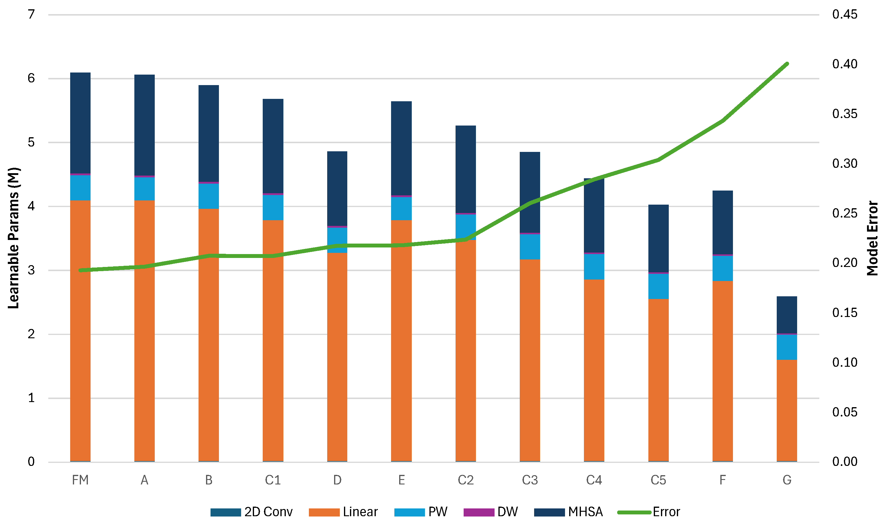
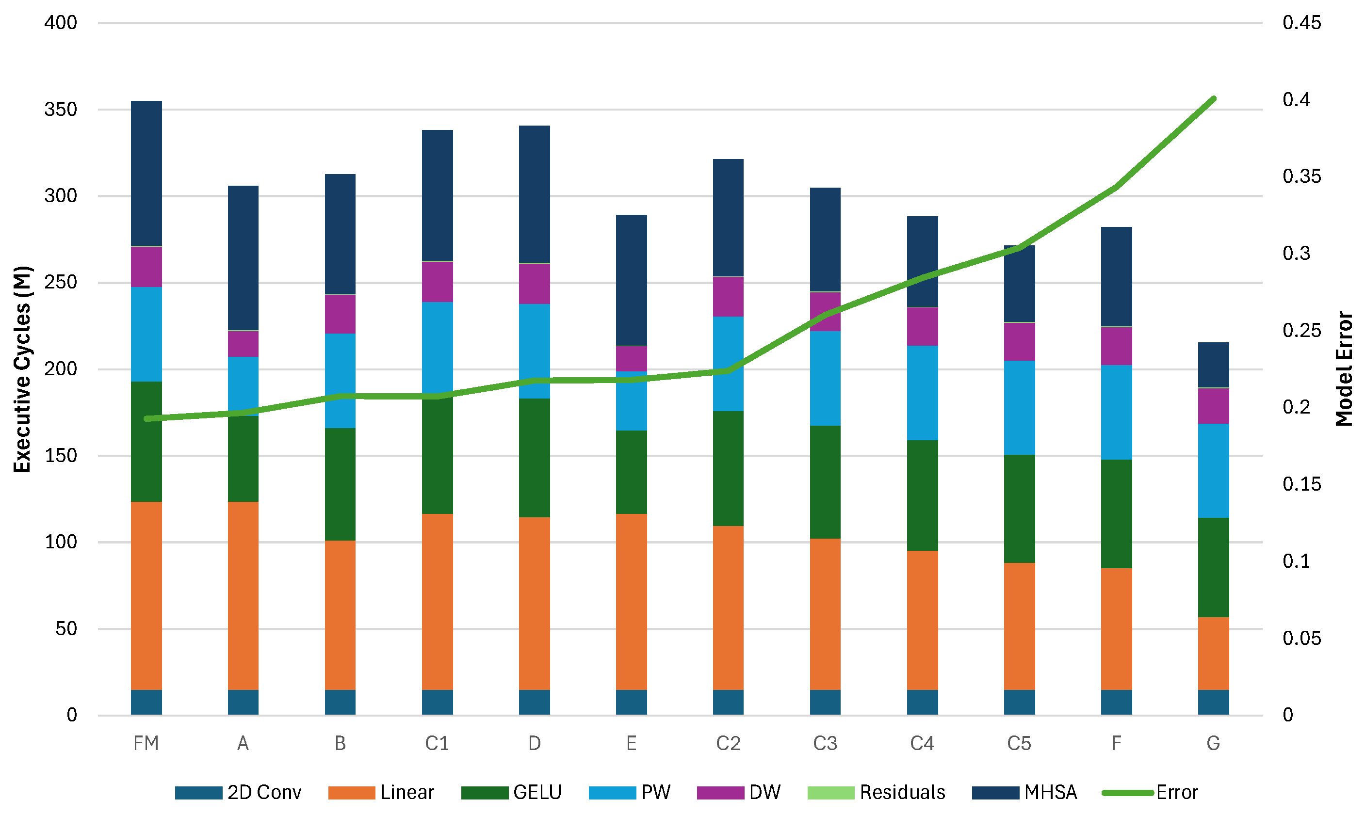
To demonstrate the effectiveness of our methodology, we present the pruning and deployment of three mobile-grade Transformer architectures: MobileBert, tinyViT, and tinyLLAMA2. For the MobileBert architecture, we have removed all but one of the encoder layers, reducing, in this way, the total memory footprint of the model by 94.9% while achieving a 19× speedup from the baseline architecture. Evaluation of the GLUE benchmark sentiment analysis task shows that this aggressively pruned version of the model retains an accuracy error (number of misclassified instances over the total) below 19% (compared to $8.9\%$ for the full model). We explore accuracy/efficiency tradeoffs for the TinyViT model by removing some of the Attention blocks from varying depths in the architecture. We show that we can reduce the memory footprint for learnable parameters and inference latency up to ∼57% and ∼39%, respectively, by pruning all encoders but with an increase of ∼20% of final accuracy error compared to the original model. A possible tradeoff is pruning only the last encoder, achieving ∼20% memory reduction while limiting the accuracy loss to ∼2.5%.

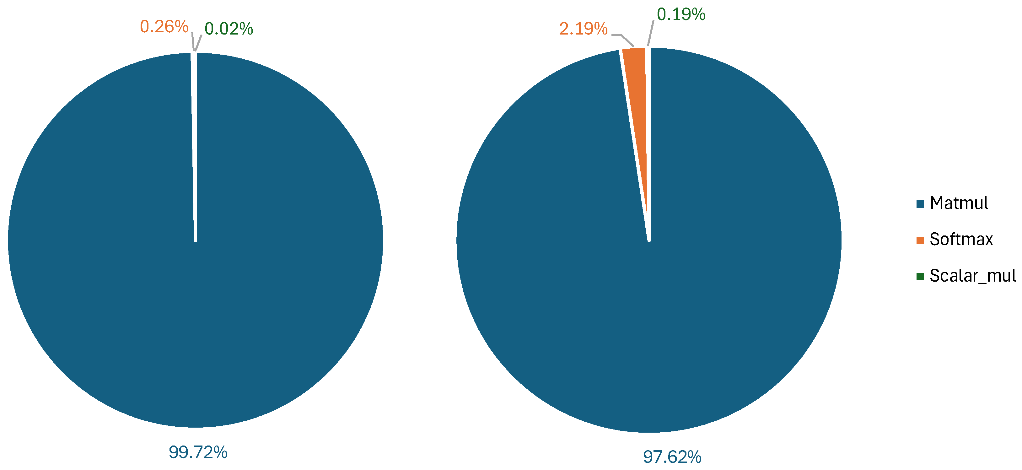
Lastly, for tinyLLAMA2, we start from a model that is already adequately small [12], and we focus on inference speed. Our optimizations reduce the total number of cycles required for the generation of 256 tokens from $5.5\times {10}^8$ to only $5.1\times {10}^7$ cycles—a ∼10× improvement. In particular, on matrix multiplications, which represent ∼50% of the total amount of operations in the network, we achieve an 18.7× speedup.

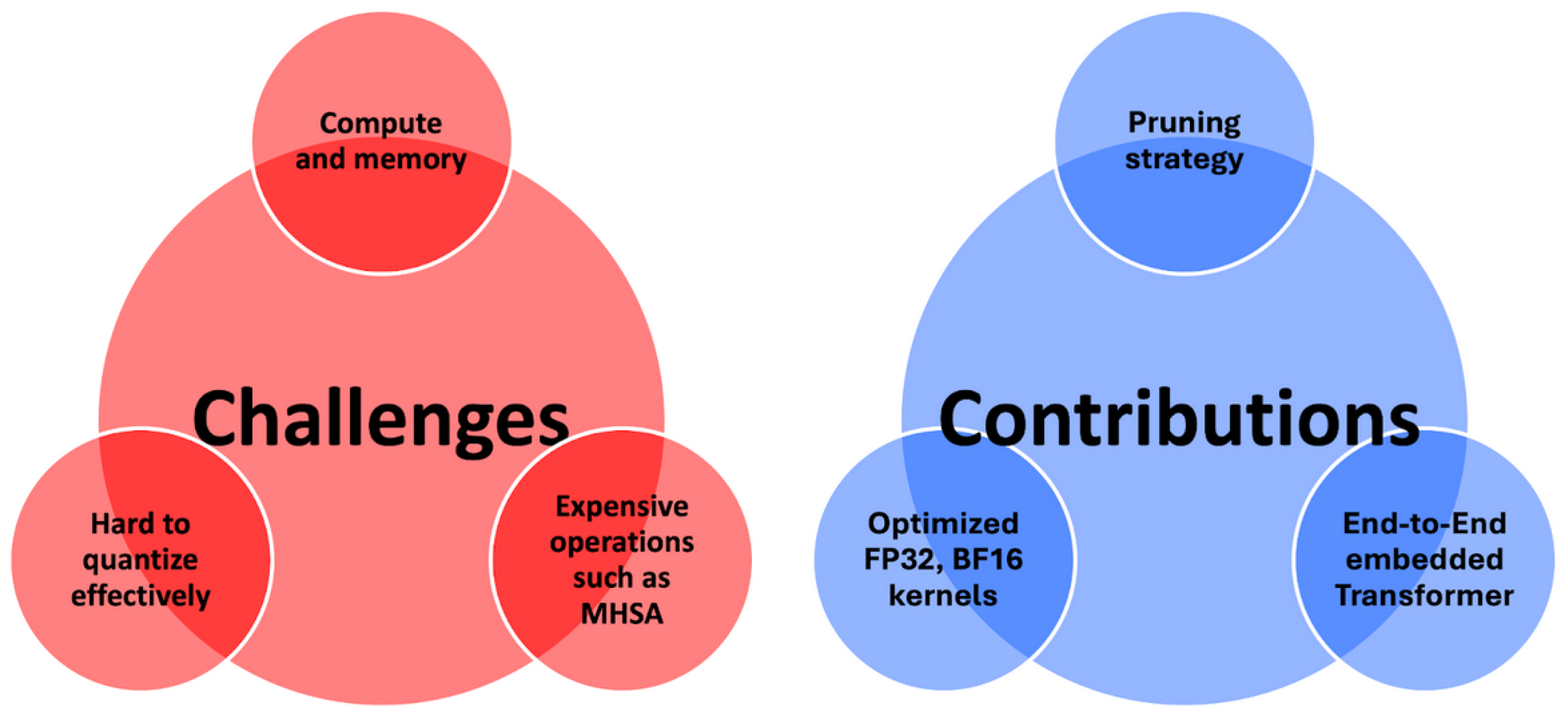
In summary, this work makes the following novel contributions, also summarized in the conceptual diagram in Figure 1:

• A methodology for deploying Transformer-based models on resource-constrained platforms without reliance on aggressive quantization techniques.
• An analysis of pruning techniques for encoder layers to reduce memory and energy footprints with controlled accuracy loss.
• Experimental results on MobileBert, tinyViT, and tinyLLAMA2, demonstrating the practicality and effectiveness of our approach.

By addressing both architectural inefficiencies and operational bottlenecks, our work lays the foundation for scalable, efficient, and accurate Transformer deployments, bridging the gap between the computational demands of this class of architectures and the limitations of ultra-low-power hardware, enabling Transformer-based applications in scenarios previously deemed impractical due to resource constraints. We release all of our methods and results as open-source code at https://github.com/Dequino/pulp-trainlib/tree/jlpea (accessed on 1 February 2025).

The rest of this paper is structured as follows: In Section 2, we discuss current techniques for efficient Transformer deployment, focusing on approaches based on quantization and pruning. Section 3 provides an overview of the fundamental operations in Transformer architectures. In Section 4, we present the optimizations introduced in this work. Section 5 outlines the results obtained for the selected architectures, demonstrating the effectiveness of our approach. Finally, Section 6 summarizes our work.

2. Related Work

Deploying Transformer models on low-power devices, such as microcontrollers, necessitates optimizations to address their limited computational resources and stringent energy constraints. One prominent approach is quantizing networks into low-bit integer formats, such as INT8 or INT4. Quantization reduces the memory footprint of the network and eliminates the need for complex hardware capable of floating-point operations, enabling inference on cheaper and more energy-efficient hardware. By quantizing floating-point computations into integer arithmetic, faster execution and lower energy consumption can be achieved. Thus, quantization has become a key strategy for deploying Transformers on resource-constrained devices. An example is I-BERT [13], which uses a fully integer-based implementation for Transformer operations, approximating the GELU and softmax operations of the BERT architecture with second-order polynomials. A similar quantization scheme is adopted in SwiftTron [14] to apply to a matrix multiplication accelerator.

Other methods relying on integer-quantization are Sparse-Quantized Representations (SpQRs) [15], in which weights are quantized mostly to 3–4 bits except for the outliers, which are identified as those weights that cause the highest quantization error, which are kept in the float16 format, allowing the execution of a large language model on consumer-grade GPUs. Other quantization methods are Generative Pre-trained Transformer Quantization (GPTQ) [16] and Optimal Brain Quantization (OBQ) [17], which aim to find a quantization scheme that reduces the squared error between the outputs of each layer before and after quantization. GPTQ adopts a block-wise approach, grouping multiple rows of weights and quantizing them to increase computational efficiency. In contrast, OBQ processes the weights row by row, starting with those that have the least impact on the overall quantization error, making it more fine-grained than GPTQ but far less computationally efficient, employing the same amount of time to quantize a model 100× smaller.

For deploying Quantized Neural Networks, Tiny Transformer (TinyFormer) [18] introduces a comprehensive workflow. It starts with a floating-point PyTorch model, exported as an Open Neural Network Exchange (ONNX) graph. The deployment tool DORY [19] then processes the ONNX graph to generate optimized C code. This code relies on an extended quantization-aware library to minimize data transfer overhead and maximize data reuse. This approach makes TinyFormer’s deployment workflow the closest point of comparison to our work in the literature.

Another approach to achieving efficiency focuses on pruning the Transformer network architecture. Unlike quantization, which reduces the precision of activations and weights by changing the data type and using fewer bits for representation, pruning focuses on simplifying the model’s topology. It removes less important parts of the model to reduce its size and computational cost, including layers or individual weights, often making it more efficient for inference while retaining the computation in floating-point precision. Despite these differences, both methods aim to improve efficiency while preserving accuracy.

Pruning is mostly divided into two categories: structured and unstructured pruning. In structured pruning, the elements removed from the network follow specific patterns like layers or groups of weights. Some methods include ShearedLLaMa [20], which applies structured pruning to a pre-existing LLM model by posing the pruning problem as a constrained optimization problem. The method eliminates layers and parameters from the starting model while retaining the original accuracy.When tested on the LLaMa model, the method achieves the best average accuracy on the lm-evaluation-harness [21] using only 50 Giga tokens from the original 2 Tera tokens training set. Another method, HOMODISTIL [22], starts from a pre-trained architecture and iteratively removes features from each layer in the network while minimizing the difference between the pruned model and the original output. Applied to the BERT Transformer model, the method reduces the total number of parameters by 35%, losing only 0.8% in average accuracy across six different tasks.

Unstructured pruning, on the other hand, eliminates individual weights within the network. Although it offers finer granularity than structured pruning, it can result in sparse weight matrices, which are more challenging to exploit on general-purpose hardware without specialized libraries. Some examples include Wanda [23] and SparseGPT [24]. Both of these methods individuate the weights that impact the output inside the networks less, removing them from the architecture. Both methods allow a reduction of up to 50% of the total weights while causing an accuracy drop that, depending on the original size of the Transformer, can be up to 5% of the original accuracy. Our work focuses on reducing the entire network structure instead of applying quantization. This approach prevents the significant degradation that is often associated with post-training integer quantization in lower-capacity models. By pruning less critical layers in the network architecture, we achieve an efficient design that maintains an accuracy comparable to the baseline model while significantly reducing the total number of parameters and operations without requiring expensive (and often unaffordable) retraining from scratch.

Furthermore, adopting a floating-point format enables our deployed architectures to exploit the existing software infrastructure. Our work extends the PULP-Trainlib [25], a software open-source framework for high-performance deployment and training of DNNs (Deep Neural Networks) on RISC-V multi-core devices, to support Transformer models.

This library stands out from other frameworks, such as AIfES [26], which exclusively uses 32-bit floating-point precision. Instead, it is designed to support 32-bit and 16-bit floating-point precision, allowing computational energy and memory reduction with respect to FP32 only, while maintaining high accuracy on IoT (Internet of Things) devices without requiring more fragile integer quantization. In contrast, other libraries such as PULP-NN [27] are designed exclusively to deploy Quantized Neural Networks in mixed precision, working on 8-bit or lower integer precision. Furthermore, Pulp-Trainlib heavily leverages parallelization and hardware-specific optimization, such as SIMD instructions and non-blocking DMA memory transfers, to enable an almost linear speedup when executing the workload on multiple cores. It also includes a tunable testing environment for profiling and validating singular NN-related kernels and complete ML models.

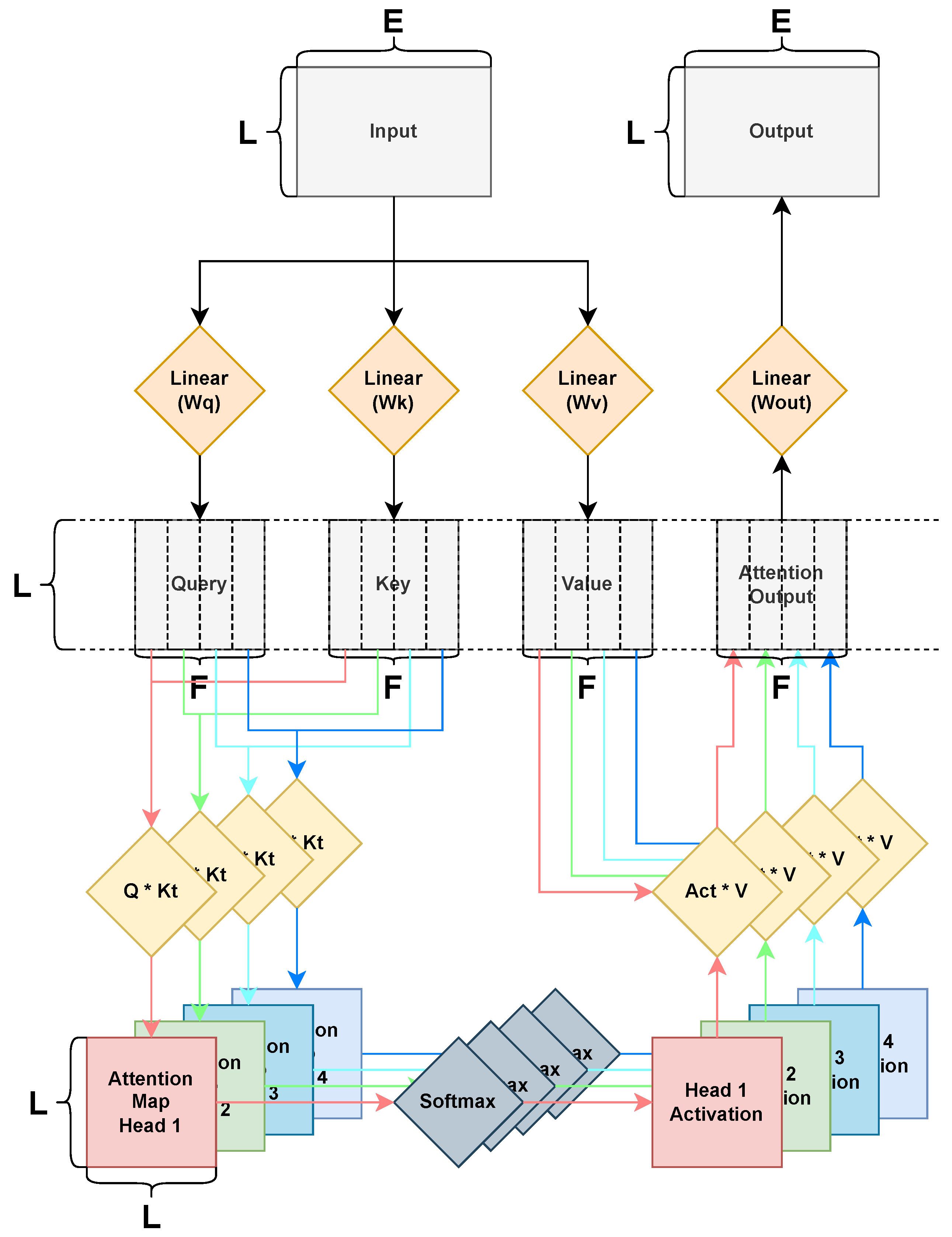
In our work, we extend Pulp-Trainlib to also include Multi-Head Attention, which we leverage for deploying three different Transformer architectures. In the next section, we will provide the necessary background to understand the main building blocks of the Multi-Head Attention kernel, while in Section 4, we will describe the optimization performed on the Multi-Head Attention kernel and their impact on performance.

3. Attention Background

3.1. MHSA Kernel

Transformer models leverage the Attention mechanism [28] for modeling dependencies in data sequences. In particular, Multi-Head Attention enables sequence analysis on multiple representation subspaces. Attention is applied to three vectors, called “queries”, “keys”, and “values” (Q, K, V). These are projections of sequential data passed as input, such as sequences of text language tokens, images or video frames, voice samples, or the output of a previous Attention block. When queries, keys, and values are projections of the same input sequence, Attention is denoted as “Self-Attention”.

Many Transformer models, especially encoder-only models, rely on multi-head computation and Self-Attention; this scenario is classified in the literature as “Multi-Head Self-Attention” or MHSA. Figure 2 shows a visual representation of the MHSA algorithm on a generic data sequence of L elements, with an embedding size of E, linearly projected on queries, keys, and values with a projection shape of F, which can be different from the original embedding dimension. First, the input is projected to Q, K, and V using separate trainable weights and biases:

$$Q=(Input\ast W_q)+b_q$$

$$K=(Input\ast W_k)+b_k$$

$$V=(Input\ast W_v)+b_v$$

Next, we match the queries and keys in a multi-head fashion by splitting the tensors on the projection shape by the number of heads, resulting in n_head sub-tensors of shape $L\times H$, where H is ${\displaystyle \frac{F}{n\text{\_}heads}}$. We then multiply each ith Q chunk with the corresponding ith K chunk, transposed for shape consistency, resulting in n_head square Attention Maps (A) of shape $L\times L$.

$$A_i=Q_i\ast K_i^t$$

Each map is passed through the Softmax activation described more in detail in Section 3.2, maintaining the same shape. Each “activated” map is matched against the corresponding ith chunk of the V tensor, which is also split in the same fashion as the Q and K vectors, generating the chunks composing the Attention Output tensor (S), that gets appended sequentially resulting in the same $L\times F$ dimension of the projection tensors.

$$S=(Softmax\left(A_1\right)\ast V_1,\dots ,Softmax\left(A_i\right)\ast V_i)$$

Finally, the Attention output is projected back to the original input sequence shape using trainable weight and bias parameters.

$$Output=(S\ast W_{out})+b_{out}$$

As we demonstrate experimentally in Section 5.2, matrix multiplications are the vast majority of the computational load of the MHSA algorithm. Therefore, we focus on optimizing its execution latency while minimizing its memory footprint to be suitable for deployment on MCUs for Edge AI.

3.2. Softmax

Softmax is one of the key operators of Transformer models, acting as their non-linear activation function of choice. It is generally defined on an n-length vector as:

$$Softmax{\left(x\right)}_i={\displaystyle \frac{e^{x_i-max\left(x\right)}}{{\sum }_{j=1}^n{e}^{x_j-max\left(x\right)}}}$$

It functionally produces a vector of the same shape as its input but whose element values sum up to 1. In most Transformer architectures, softmax is applied row-wise over the Attention maps. Figure 3 shows its implementation. This activation can be computationally expensive, requiring multiple memory accesses and data movements on the Attention map for maximum search and row summation. It also has a memory overhead due to the support buffers required for storing the intermediate values. While the maximum search is not mathematically necessary to calculate Attention, it reduces numerical problems in the subsequent exponential function; by subtracting the max from all elements, the exponent is always zero or a negative number. Fortunately, as there are no data dependencies between rows, it is easy to parallelize the workload of each operation on the sequence length shape.

Another issue the softmax poses is the exponential function, which is expensive on lower-end platforms like the one chosen as a target. We choose the Schraudolph [11] approximation function for its simplicity and because its limitations are acceptable in our chosen precision format. Considering the FP32 precision format, to calculate $y=2^x$, we can consider x as the “exponential” part of y, placing it starting from the 23rd bit. If we use the y bits as representing an integer (that we denote as $I_y$), we can calculate it as:

$$I_y=2^{23}\ast (x+127)$$

By exploiting the logarithmic property:

$$e^x=2^{x {log}_{2}e}=2^{x{\displaystyle \frac{lne}{ln2}}}=2^{{\displaystyle \frac{x}{ln2}}}$$

The previous formula becomes:

$$I_y=2^{23}\ast ({\displaystyle \frac{x}{ln2}}+127)$$

Pseudocode of Schraudolph algorithm is:

  float fastexp_exps(float x){

  x = EXPS_A * x + EXPS_B;

  if(x < EXPS_C x > EXPS_D)

      x = (x < EXPS_C) ? 0.0f : EXPS_D;

  uint32_t n = (uint32_t) x;

  return *(float*) &n;

  }

We save ${\displaystyle \frac{2^{23}}{ln2}}$ and $2^{23}\ast 127$ as constant values (EXPS_A and EXPS_B) for accelerating this operation, and we also save $2^{23}$ and $2^{23}\ast 255$ as constant limit values (EXPS_C and EXPS_D) to verify the algorithm applicability. When working with FP16 data, we found that casting 32 bits to use the method described above was slightly faster than using the same algorithm while maintaining the same accuracy.

4. Platform and Methods

4.1. PULP Platform

The PULP (Parallel Ultra-Low Power) platform is an architecture designed for lower operating voltages, increasing energy efficiency but still achieving high application performance thanks to parallelism and hardware acceleration. Figure 4 shows the architectural paradigm of a commercial chip implementation of the PULP paradigm, GreenWaves’ GAP9 SoC (System-on-Chip), built upon the open-source VEGA [29] architecture, which we use as an experimental target to validate our methodology. The platform is divided into two regions with possibly different clock and voltage domains: the SoC domain and the computation cluster.

The SoC features a RISC-V FC (Fabric Controller) for managing and controlling tasks. The cluster comprises nine RISC-V cores focused on accelerating computation tasks in a parallel fashion. All the cores support the RV32IMFC ISA (Instruction Set Architecture) extended with the XpulpV2 ISA extension: a set of DSP instructions such as post-increment store/load and hardware loops. The cores have private instruction caches and follow an architectural design supporting the transprecision computing paradigm [30]. This design includes sharing and pipelining FPU units between different cores to avoid memory throughput bottlenecks. A Single-Instruction–Multiple-Data (SIMD) approach supporting instructions acting on packed-SIMD vectors, which enables us to operate simultaneously on multiple sub-word elements, in particular of the 16-bit half-precision (float16) and brain-float 16 (bfloat16), packed together and exploiting the 32-bit floating point bandwidth of the platform. No data caches are available for the cluster cores to minimize memory coherency overhead and area. Instead, a multi-banked TCDM (Tightly Coupled Data Memory) of up to 128 kBs, labeled as L1 (Level 1) memory, is used as a scratchpad, with each bank having its port allowing concurrent access to different memory regions, enabling data parallelism. Intra-cluster communication is based on a word-level interconnect with a word interleaving scheme, allowing single-cycle memory accesses to the TCDM.

The different memory levels interact through the Direct Memory Access (DMA) unit, which manages data copies in both directions in the background without interrupting any core activity. In our setup, we use the parallel cluster of nine cores to accelerate the DNN primitives composing Transformers; in particular, we use eight cores for parallelizing the workload, while the nineth is used for programming and managing the others, acting as a “cluster controller”. We also use the other platform components to efficiently schedule data movements to enable the deployment of complex Attention-based models even on a highly constrained, small embedded device.

The architecture has a rich set of I/O interfaces that adapt to various sensors and data signals, such as video or audio. An interleaved SRAM memory of up to 1.5 MBs, labeled the L2 memory, is implemented on the SoC side, accessible by the FC in a single cycle. Finally, a non-volatile MRAM of up to 4 MBs is also available.

4.2. PULP Trainlib

As Section 2 indicates, we extend the PULP-Trainlib to support Transformer architectures. To do so, we introduce kernels for Multi-Head Attention, typical of Transformers. The main operation used in this layer type is matrix multiplication.

Matrix multiplication is one of the fundamental operators in machine learning, as most data are elaborated in a vectorized form for optimizing precision and usage. Considering two input matrices (A, B) of shape $N\times K$ and $K\times M$, respectively, the output matrix of shape $N\times M$ is composed as:

$$Output[i,j]=\sum _{k=0}^{K}A[i,k]\ast B[k,j]$$

In Figure 5 and Figure 6, we show a naïve basic code implementation of this function and its disassembled form. This function can be optimized when working on an embedded PULP architecture by exploiting different software and hardware techniques.

As the matrix multiplication is a nested loop function, we can increase efficiency by enabling hardware loops from the RV32IMFC ISA. These instructions, supported by the XpulpV2 ISA extension, allow repetition of a code block while removing the overhead of branches penalty and counter updating, and also have no stall cycles for jumping. It is defined by a 32-bit aligned start and end address, pointing to the first and last instructions executed by the loop, and a counter register automatically decreases each time the last instruction is called. An example of hardware loop integration is in Figure 6. As the ISA supports at most two levels of loops, we still need to rely on branches for the outermost cycle, but this has no impact on the overall performance.

More improvements are obtained by loop unrolling, a technique in which we explicitly write multiple loop iterations of the inner loop, maximizing data reuse in the register file and reducing the overhead caused by branching. We define an unrolling factor $U\times V$, the shape of the output region being computed concurrently in the inner loop. Increasing this factor can decrease the instruction count until the generated code has to invoke the stack due to the limited number of registers. This technique also faces slowdowns when the output dimension is not divisible by the unrolling factor, requiring an external “leftover” routine to compute the edge cases.

Because there is no race condition when calculating each element of the output vector, we assign different output areas to each core of the PULP cluster to be computed, as shown in Figure 7, enabling parallelization. As data are stored in memory following the HW (height, width) shape, we split the workload on the sequence length dimension as evenly as possible to maximize data and address reuse. Data required for computing each head’s Attention Map A is organized in memory to be contiguous, optimizing reads and data transfers, essential for tiling, as explained in more detail in Section 4.3.

4.3. Data Tiling

When working with FP16 data, the RV32IMFC ISA supports SIMD instructions that allow using the 32-bit datapath to load, operate, and store on two consecutive 16-bit data elements with a single instruction each. Figure 5 shows an example of code exploiting SIMD instructions for reducing the MatMul inner loop cycle count even when using a lower unrolling factor than the FP32 version.

One of the main issues of Transformer deployment on MCUs is the model size itself, inflated by the sheer amount of trainable parameters, embedding table, intermediate maps, activation, and cached values (on generative applications) while also working on data sequences of arbitrary length, increasing the intermediate Attention map sizes. Even after pruning most redundant components for smaller tasks, as shown in Section 4.4, the memory requirements may still be too high for deploying the model directly on the memory regions close to an embedded system’s computational units. For instance, the architecture chosen for our experimental setup has a limit of 128 kBs on the L1 TCDM side, forcing us to use the larger but slower memory regions to deploy our model.

We employ a tiling strategy on the platform to improve model performance, exploiting the non-blocking DMA unit to efficiently transfer data between different memory levels. Figure 8 shows the tiling process used to optimize the computation of a linear layer. We divide the output area into sub-windows, called “tiles”, which only require a portion of the input, weights, and bias to be calculated. We reduce the tile shape enough to fit all the necessary function data in our limited L1 area, using the DMA unit to manage the correct positioning of each parameter on the memory array, as each core of the cluster has defined different entry pointers to read and write data in a parallelized fashion. As the DMA is non-blocking and can transfer data as the cluster cores are computing, it is possible to schedule the data movements to create a “pipeline” to minimize cluster wait time and maximize its efficiency. However, this strategy requires multiple buffers to avoid race conditions, which further reduces tile dimensions and might not be feasible when dealing with data with substantial embedding sizes.

Full AI models are composed of sequences of different processing blocks, each with its type and shape, with different memory footprints and mapping complexity. Therefore, we apply a dynamic tiling strategy to choose for each operation level that is the most optimal, parallelizable tile shape ($h\text{\_}tile$ and $w\text{\_}tile$ in Figure 8) aimed to maximize the L1 memory usage. For instance, for each MHSA block, we use different tiling dimensions for input projections, output projection, softmax, transpositions, $Q\ast K^t$ multiplication, softmax activations, and $A\ast V$ multiplications, all operators that are fused in our kernel implementation. We use optimization tools, namely Google’s open-source OR-Tools [31], to automate the search for fitting tiling dimensions based on the original shape for each operator, which we define as a combinatorial problem to be solved by Constraint Programming.

4.4. Encoder Pruning

While the general trend of Transformer models is to generalize as much as possible and grow in size, this exponential increase in complexity boosts model flexibility and generality but does not necessarily relate to higher accuracy and reliability on smaller and more specific tasks [32]. As deploying full size, foundational Transformers on small embedded platforms is often an unfeasible task due to their size, we investigate if it is reasonable to prune a portion of the model, particularly encoder chains, to fit the memory constraints with controlled accuracy loss. Inspired by the simple LLM pruning methodologies proposed in works such as [20,33,34], we propose a simple encoder pruning methodology to resize a generic Transformer model to a deployable size, showing its effectiveness on non-LLM models such as MobileBert and TinyViT.

Transformer architectures are commonly structured as one or more sequences of MHSA blocks acting as “data eencoders” followed by linear layers that serve as the task-specific output head. Each encoder block has the same structure but uses distinct sets of learnable weight parameters. We investigate whether every component of these sequences within these encoder sequences is indispensable for achieving the high representational capacity typically associated with Transformer models. Specifically, we focus on large mobile-class pre-trained Transformer models, which are impractical for MCU deployment due to their significant memory and computational demands. We examine the impact on model accuracy by systematically removing MHSA blocks from the encoder, starting with those nearest to the output head, following an approach summarized by the pseudocode in Algorithm 1. Although such removals typically degrade performance to near-random levels, we find that a brief fine-tuning phase on the entire new architecture consisting of a few training epochs in our chosen architectures: five epochs with learning rate $5\times {10}^{-5}$ and $1\times {10}^{-2}$ weight decay for MobileBert and 30 epochs with variable learning rate from $1.25\times {10}^{-7}$ to $6.25\times {10}^{-5}$ and $1\times {10}^{-8}$ weight decay for TinyViT, which are the same learning rates used in both the original works, both using the default AdamW optimizer, can effectively restore accuracy to a level comparable to the original model, as will be shown in the experimental results in Section 5.3 and Section 5.4 evaluated on the GLUE benchmark and ImageNet-1k, respectively. This approach allows us to find a reduced Transformer variant with significantly fewer parameters, lower memory requirements, improved latency, and reduced energy consumption while maintaining high accuracy. Crucially, this method is more efficient and less resource-intensive than designing and training a model specifically tailored for embedded deployment from scratch.

Algorithm 1 Encoder Pruning Algorithm

1: function EncoderPruning(args)   2:    $n\text{\_}kept\text{\_}layers\leftarrow args.n\text{\_}kept\text{\_}layers$   3:    old_model ← Transformer.From_Pretrained(args.pretrained_path)   4:    $new\text{\_}model\leftarrow$Transformer()   5:    new_model.Set_Config$(n\text{\_}encoder\text{\_}layers\leftarrow n\text{\_}kept\text{\_}layers)$   6:    $new\text{\_}model.embedder\leftarrow old\text{\_}model.embedder$   7:    for $i\leftarrow 1$ to $n\text{\_}kept\text{\_}layers$ do   8:    $new\text{\_}model.encoder\left[i\right]\leftarrow old\text{\_}model.encoder\left[i\right]$   9:    end for 10:    $new\text{\_}model.head\leftarrow old\text{\_}model.head$ 11:    $new\text{\_}model\leftarrow$ Finetune(new_model) 12:    return $new\text{\_}model$ 13: end function

5. Results

5.1. Experimental Setup

To validate our methodology, we evaluate our kernel performance on GVSOC [35], a highly configurable timing-accurate simulation environment for RISC-V-based architectures tuned to target the GAP9 SoC, and on a physical commercial board, the GapMod, equipped with the same GAP9 SoC. We study the reduction and deployment of three different tiny-Transformer encoder-based models on this board: MobileBert [36] and TinyVit [37] for non-generative/classification tasks, and tinyLLAMA [38] for generative tasks.

5.2. MHSA Kernel

The MHSA kernel, introduced in Section 3.1 and Figure 2, is the principal component of encoder-based Transformer models. By exploiting the optimization techniques described in Section 3.2, Section 4.2 and Section 4.3, we improved this component starting from a C porting of PyTorch’s primitives. Figure 9 exemplifies the singular kernel improvements on a test case of a sequence of 64 elements with an embedding size of 512, both in the 32 and 16-bit floating-point versions. Following the PULP’s cluster architecture, parallelization results were obtained on 8 RISC-V cores. We compare a fully deployed kernel version on a larger L2 memory and a second version using a dynamic tiling scheme, introduced in Section 4.3, to calculate the best operation-level tiling solution that fits the L1 TCDM constraints described in Section 4.1. The Y-axis is on a logarithmic scale of base 10 to facilitate visualization of the different optimization techniques applied. Numerical values are shown in

Table 1. MACs/cycle experimental results of Figure 9. Parallelization and L1 dynamic tiling are the major contributors to improving the kernel’s performance.

Precision	Naïve	Naïve + L1 Tile	MM Opt. + HW Loops	MM Opt. + HW Loops + L1 Tile	Parallel.	Parallel. + L1 Tile
FP32	0.03	0.14	0.08	0.54	0.63	3.30
FP16	0.03	0.14	0.16	1.01	1.26	6.29

.

Considering all the improvements, in this example, the optimized implementation for FP32 is more than $116\times$ faster than the initial naïve C port of PyTorch’s MHSA kernel. In comparison, the FP16 version is improved by more than $220\times$. Significant contributors to this speedup were the following: parallelizing the workload, which led to an almost linear speedup of the kernel ($7.88\times$ for the FP32 version, $7.97\times$ for the FP16 version) very close to the theoretical maximum of $8\times$ speedup and dynamic tiling between different memory levels, improving the parallelized kernels by $5\times$ on average. The 16-bit kernels show improved results compared to the 32-bit ones due to a combination of the usage of SIMD instructions, as explained in Section 4.2 and in Figure 5, and the possibility of using larger tiling factors due to the reduced number of bytes per element, minimizing the number of data transfers in between memory levels and maximizing data reuse at runtime. We validated the correctness of our software kernels by ensuring the numerical results align with the outputs of the equivalent PyTorch methods with FP arithmetic, used as the “golden model” for validation.

Figure 10 and

Table 2. MACs/cycle experimental results of Figure 10.

	MatMul	Softmax	Scalar Mul.
MACs/FLOPs	$7.14\times {10}^7$	$1.83\times {10}^5$	$1.63\times {10}^4$
Active Cycles	$1.11\times {10}^7$	$2.49\times {10}^5$	$2.10\times {10}^4$

show the distribution of the primitives composing the MHSA kernel, both in terms of Multiply and Accumulate (MAC) or Floating Point Operations (FLOPs) on the left graph, and the number of runtime cycles when deployed on the right. MACs and active cycles were counted on the most optimized version of the solution using the same testing parameters chosen for Figure 9. In both graphs, the MatMul algorithm overwhelmingly dominates, with $99.72\%$ MACs dedicated to them, justifying our effort on optimizing this part of the execution and $97.62\%$ of active cycles during runtime. Although this difference in distribution may appear small, it denotes an inefficiency in Softmax activation, whose share increases about $8.4\times$ (from $0.26\%$ in MAC to $2.19\%$ in cycles), even after approximating and parallelizing the expensive exponential function, as described in Section 3.2.

Figure 11 shows the MACs/cycle values obtained by changing both the input sequence length and hidden Attention projection size while keeping the same number of computational Attention heads and input embedding dimension at 4 and 512, respectively, which are the same parameters used by each MHSA layer of the MobileBert encoder. The overall kernel performance is reduced when working with smaller projection sizes due to the multi-head data splitting on the projection size shown in Figure 2, which leads to creating data chunks with shapes that may ill-fit the optimization techniques used so far. For instance, the unrolling strategy for optimizing memory accesses on contiguous data on matrix multiplications stops being viable on parallelized workloads if there are not enough elements to unroll in the first place. We must use less optimized element-wise multiplicative operations and data accesses in this case. Moreover, tiling is also limited by the current operands’ shape: a high number of small data transfers is less effective than completing a smaller number of more extensive data transfers due to the overhead caused by the calls to the DMA unit. Therefore, we generally have higher performance when dealing with higher data density and larger kernel sizes; however, by increasing the sequence length size, the overhead caused by the Softmax activation starts having a more significant impact on the performance: this is caused by the increased shape of the Attention Maps $A_i$ (of shape $L\times L$, as explained in Section 3.1), which, as shown in Figure 3, has to be accessed multiple times, element by element, for calculating row-wise maximum, sums, and exponential values.

We compare our solution’s performance against two state-of-the-art inference libraries for PULP architectures, PULP-NN [27] and the Tiny Transformer (TinyFormer) deployment flow [18]. Experimental results are shown in Figure 12, in which we compare execution cycles of the MHSA kernel using different numbers of parallel cores on GAP9. For a fair comparison with the results available in the cited works, input sequence length, embedding size, and single-head hidden dimension were all set to 64, and the number of heads was set to 8. Because PULP-NN is designed to work on mixed-precision data, whereas TinyFormer is a workflow designed for deploying Quantized Neural Networks (QNNs), we compared their performance on int8-precision, as it is the only experimental data available in their work, despite our experiments being executed on FP32 and FP16-precision data. Due to the data size difference, our FP32 kernel is ∼3.9× slower than TinyFormer, whereas the FP16 kernel is ∼2.3× slower. Compared to PULP-NN, however, despite working with larger data items, our FP32 solution has similar performance on eight parallel cores, while our FP16 kernel is ∼1.7× faster, proving that our methodology has a more optimized parallelization strategy.

5.3. MobileBert Deployment

As discussed in Section 4.4, we study the possibility of reducing the memory requirements and latency for the Transformer model to be deployable in a restricted embedded device while maintaining a level of accuracy comparable with the original version. We use a basic MobileBert model as a study target for sequence classification. The original model configuration includes 24 encoder blocks, each composed of a trainable 4-head MHSA kernel and a 2-stage Feed-Forward Network (FFN) bottleneck layer, operating with a hidden projection size of 128 elements. The encoder sequence is preceded by an embedding stage on the token values, positions, and types, using a set of three dictionaries, the first of 30,522 entries for the token values, up to 512 entries for the positions, and two different entries for token types. The input embedding size is 512 elements. After the encoding part, a linear classification head returns the final result of the model.

In order to meet the memory requirements for model deployment, we reduced the number of layers in the Encoder chain by pruning each block, starting from the one closest to the classification head, before any form of fine-tuning on the downstream task, as explained in Section 4.4. Figure 13 shows the trainable memory requirements versus runtime latency versus accuracy error calculated on the GLUE benchmark’s sentiment analysis task for text sequences. By pruning all but one encoder block, it is possible to reduce memory requirements up to $94.9\%$ compared to the baseline model while improving latency by about $19\times$, keeping the accuracy error below 0.19 and not degenerating the model to random guessing, which is noteworthy considering the baseline model error is 0.084. We can limit the accuracy drop by pruning the encoder to twelve blocks, reducing memory requirements by $49.5\%$ and improving latency by about $2\times$, without any noticeable error increase in the model. Furthermore, we highlight that halving the number of encoder layers has little to no effect on the overall accuracy, showing a redundancy in the model design that hinders deployment on lower-end platforms for minimal benefits on the task itself.

Figure 14 and

Table 3. The MACs and cycle experimental results of Figure 14.

	Padding	Embedding	Matmul	Norm	Softmax	Add	Relu	Overhead
MACs	$4.91\times {10}^4$	$1.47\times {10}^5$	$1.36\times {10}^8$	$4.91\times {10}^5$	$7.27\times {10}^5$	$2.78\times {10}^5$	$2.62\times {10}^5$	-
Cycles	$2.62\times {10}^4$	$5.71\times {10}^4$	$2.42\times {10}^7$	$3.61\times {10}^5$	$1.04\times {10}^6$	$4.11\times {10}^5$	$5.52\times {10}^5$	$2.92\times {10}^5$

denote the distribution of MAC operations and cycles of the deployed Reduced MobileBert with a single encoder layer. Despite reducing the number of MHSA kernels from 24 to 1 and using the full model, including different kinds of non-Transformer blocks in its architecture, matrix multiplication is still the most computed operation, with more than $98\%$ of the total MACs dedicated to it, proving how important it is to focus on optimizing this component. On the cycle side, the distribution changes due to a difference in optimization on the different operations: while our efforts proved to be effective on MatMuls, non-linear activation functions, such as Softmax and ReLu, are more challenging to optimize with a software-based approach, and may require more hardware-focused solutions such as Accelerators.

5.4. TinyVit Deployment

TinyViT [37] is a family of image classification models pre-trained on large image datasets and fine-tuned on smaller tasks through distillation. In Figure 15 and

Table 4. MACs and cycle experimental results of Figure 15.

	2D Conv	Linear	GELU	PW Conv	DW Conv	Residuals	MHSA
MACs	$6.86\times {10}^7$	$5.44\times {10}^8$	$1.57\times {10}^8$	$2.80\times {10}^8$	$1.95\times {10}^7$	$1.24\times {10}^6$	$3.79\times {10}^8$
Cycles	$1.50\times {10}^7$	$1.08\times {10}^8$	$6.93\times {10}^7$	$5.45\times {10}^7$	$2.35\times {10}^7$	$4.63\times {10}^5$	$8.32\times {10}^7$

, we show the distribution of the internal operations of the base TinyViT-5M model, both in the number of MACs and operative cycles, using extended PULP-Trainlib kernels. The model is structured in several different operating regions: first, the input image is embedded through two 2D Convolutional layers and a GELU activation, followed by two MobileNetV2-like bottlenecks. Next, the input is down-sampled via two Point-Wise Convolutions, one Depth-Wise Convolution, and another GELU Activation before entering the first Encoder region. This region comprises two “TinyViT” blocks: each includes an MHSA block, an MLP, and a depth-wise Convolutional layer. After a second down-sample process, another Encoder region is reached, composed of six TinyViT blocks following the same overall architecture of the previous region but with a completely different hidden Activation shape. Data are down-sampled a third time before accessing another and final Encoder region composed of two TinyVit blocks with new inner Activation shapes. The output is then passed to a Linear head for classification.

Most notable is that the dominating operation is not the Attention mechanism but the linear layers composing the Multi-Layer Perceptron (MLP) networks between the Transformer blocks, thus increasing the need to optimize the MatMul primitive. The cycles follow a similar distribution of the MAC operations, with an increased percentage of Depth-Wise convolutions and GELU activations while reducing the share of the remaining operations caused by the difficulty of optimizing non-linear operations like the GELU and the impossibility of exploiting data reuse when working with depth-wise convolutions. On average, our framework reaches a rate of 4.09 MACs/cycle on the full TinyViT-5M model.

As we did for the MobileBert in Section 5.3, we studied the possibility of reducing the model via a cropping mechanism. However, due to the particular architecture of TinyViT composed of multiple, different Encoder regions, we adopted a different search strategy: We studied the impact on accuracy evaluated on the ImageNet-1k dataset for removing MHSA blocks from each region independently, removing blocks concurrently from multiple regions, and also analyzed the impact on performance by removing part of the MobileNet-like Embedder.

Figure 16 shows the memory saving and accuracy for the different reduced models we tested, whereas Figure 17 shows their performance in terms of millions of cycles. Just like in the previous model, removing blocks closer to the Linear Head has a lesser impact on the final accuracy, whereas removing multiple blocks from different areas, while producing a significant reduction to the memory footprint, can end up doubling the final error of the model. We can infer that our pruning methodology is less effective for TinyViT compared to MobileBert, as the most aggressive pruning, which reduces each encoder region to a single MHSA block, achieves a $57.4\%$ reduction in memory usage and $1.6\times$ latency improvement but also increases the model’s error by $2\times$. A possible trade-off can be found by pruning fewer encoder layers and by focusing on the layers closer to the head classifier; for example, cropping the third encoder alone achieves a $20.2\%$ decreased memory usage and improves the inference time by $1.04\times$ while limiting the error increase to $1.1\times$.

We also present in Figure 18 the average confusion matrix for the first 50 classes, computed across all pruned models.

5.5. tinyLLAMA Deployment

Large Language Models (LLMs) are Transformer-based models specialized in elaborating natural language, usually trained over immense datasets to be used for most generic applications. Llama2 [39] is an open-source subset of LLMs that are decoder-only and present some core differences from classic LLMs that enable model size reduction and execution complexity, such as the $KVcache$, which memorizes the Keys and Values projections shared by multiple heads so that they do not need to be computed again on each iteration, using RMSNorm instead of the classic Layer Norm, Swish-Gated Linear Unit (SwiGLU) instead of the ReLU, and a positional encoding based on the relative position of the token, called “Rotary Positional Embedding” (RoPE) [40]. These methods paved the way to studying how small a language model can be while keeping the ability to generate comprehensible English text, the so-called “Small Language Models” (SLMs), by training over reduced datasets, such as TinyStories [41].

We study the deployment of one of these SLMs, pre-trained on TinyStories, on GAP9, using our extended PULP-Trainlib to optimize inference. The model follows a simple architecture composed of an encode step over the prompt and a sequence of MHSA forward, sample, and decode steps to generate the token sequence. Each forward block comprises five MHSA layers, each composed of eight heads and an internal projection size of 64, separated by FFNs, resulting in a final model of just 260 k learnable parameters (688 KBs in FP16 precision). Since this model fits our chosen target well, we do not need to apply any pruning technique like in the previous architectures.

The experimental FP32 and FP16 results listed in

Table 5. Experimental cycles for each component of deployed tinyLLAMA. Cycles for the forward part have been counted for a single head and layer when generating the 256th token, as it is the most computationally complex since it considers all previously generated tokens. Total cycles counts all of the cycles to generate the entire token sequence.

Function			FP32 Cycles	FP16 Cycles
encode			321,424	321,268
$\times 256$ steps:
forward	$\times 5$ layer	RMSNorm	542	663
		V Projection	1247	804
		Q Projection	1920	1139
		K Projection	1185	831
		RoPE	3511	3478
		$Q\ast K^t$	9328	6585
		Softmax	14,159	14,398
		$A\ast V$	5367	4310
		Out Projection	1975	1190
		Residual 1	185	193
		RMSNorm	697	717
		FFN MatMul 1	4771	2650
		FFN MatMul 2	4707	2635
		SwiGLU	2122	2200
		FFN MatMul 3	3667	1999
		Residual 2	204	200
	Final RMSNorm		724	587
	Final Projection		16,807	8701
sample	Softmax		3097	3127
	Sample top-p		15,396	7090
decode			58	885
Total cycles			75,107,449	51,954,140

were obtained when generating a 256 token-long text using “Tim was very happy” as the initial prompt. We exploited all the optimization techniques introduced so far and used the “Coordinate Rotation Digital Computer” (CORDIC) algorithm to approximate the $cosf$ and $sinf$ operations in RoPE. As each token generation considers the previous ones, we show the performance of the forward function on the last generated token, as it is the most computationally intensive task of the model. “Total cycles” is the final count to generate the complete token sequence.

We also show a power profiling of the model deployed on the GAP9 platform on different working frequencies, as shown in Figure 19 and in

Table 6. Experimental results of Figure 19.

	Execution Time [ms]	Avg. Power [mW]	Peak Power [mW]
50 MHz	1549	14.99	29.9
185 MHz	419	31.95	48.42
370 MHz	210	57.85	87.75

, by analyzing the current on the 1.8 V port of the DC-DC internal converter, which powers the entire logic of the internal cores and memory. We ignored the sequence printing stage, as it depends on the serial communication standard chosen. When using a frequency of 370 MHz, we achieve a final throughput of 1219 tokens per second, with an energy consumption of just 47.5 uJ per token. This is the point of highest work efficiency measured on the nominal board tension of 0.8 V. It is less influenced by the static parasitic power component of ∼7.85 mW, obtainable by linearly regressing the results shown in Table 6.

6. Conclusions

In this work, we paved the way for the deployment of Tiny Transformers on extreme edge MCUs, without relying on integer quantization schemes, by developing software kernels that achieve up to $220\times$ better performance than naïve C implementations of PyTorch MHSA kernels on BFloat16 accuracy, and by using extensive pruning search, exploiting the intrinsic redundancy of Transformer models. In particular, we demonstrate our deployment methodology on three Transformer-based models: MobileBert, with a memory footprint reduced by $94\%$ and $19\times$ improved latency with an accuracy degradation of $10.2\%$; TinyViT, with memory footprint reduced by up to $57\%$ and $39\%$ reduced latency, but with an accuracy degradation of $21\%$; and tinyLLAMA, which did not require model reduction and achieved a throughput of 1219 tokens per second with an energy consumption of 47.5 uJ per token. Our work sets the foundation for deploying high-performance non-quantized Transformer models on commercial off-the-shelf parallel MCUs, showing the possibility of enabling high-accuracy AI capabilities even on cheaper, low-power devices.

References

1. Brown, T.; Mann, B.; Ryder, N.; Subbiah, M.; Kaplan, J.D.; Dhariwal, P.; Neelakantan, A.; Shyam, P.; Sastry, G.; Askell, A.; et al. Language Models are Few-Shot Learners. In Proceedings of the Advances in Neural Information Processing Systems, Online, 6–12 December 2020; Larochelle, H., Ranzato, M., Hadsell, R., Balcan, M., Lin, H., Eds.; Curran Associates, Inc.: New York, NY, USA, 2020; Volume 33, pp. 1877–1901. [Google Scholar]
2. Touvron, H.; Lavril, T.; Izacard, G.; Martinet, X.; Lachaux, M.A.; Lacroix, T.; Rozière, B.; Goyal, N.; Hambro, E.; Azhar, F.; et al. LLaMA: Open and Efficient Foundation Language Models. arXiv 2023, arXiv:abs/2302.13971. [Google Scholar]
3. Dosovitskiy, A.; Beyer, L.; Kolesnikov, A.; Weissenborn, D.; Zhai, X.; Unterthiner, T.; Dehghani, M.; Minderer, M.; Heigold, G.; Gelly, S.; et al. An Image is Worth 16 × 16 Words: Transformers for Image Recognition at Scale. In Proceedings of the International Conference on Learning Representations, Vienna, Austria, 3–7 May 2021. [Google Scholar]
4. Carion, N.; Massa, F.; Synnaeve, G.; Usunier, N.; Kirillov, A.; Zagoruyko, S. End-to-End Object Detection with Transformers. In Proceedings of the ECCV, Glasgow, UK, 23–28 August 2020. [Google Scholar]
5. Baevski, A.; Zhou, H.; Mohamed, A.; Auli, M. wav2vec 2.0: A Framework for Self-Supervised Learning of Speech Representations. arXiv 2020, arXiv:abs/2006.11477. [Google Scholar]
6. Yang, D.; Tian, J.; Tan, X.; Huang, R.; Liu, S.; Chang, X.; Shi, J.; Zhao, S.; Bian, J.; Wu, X.; et al. UniAudio: An Audio Foundation Model Toward Universal Audio Generation. In Proceedings of the ICML 2024, Vienna, Austria, 21–27 July 2024. [Google Scholar]
7. Xiao, B.; Wu, H.; Xu, W.; Dai, X.; Hu, H.; Lu, Y.; Zeng, M.; Liu, C.; Yuan, L. Florence-2: Advancing a Unified Representation for a Variety of Vision Tasks. In Proceedings of the 2024 IEEE/CVF Conference on Computer Vision and Pattern Recognition (CVPR), Seattle, WA, USA, 16–22 June 2024; pp. 4818–4829. [Google Scholar] [CrossRef]
8. Radford, A.; Kim, J.W.; Hallacy, C.; Ramesh, A.; Goh, G.; Agarwal, S.; Sastry, G.; Askell, A.; Mishkin, P.; Clark, J.; et al. Learning Transferable Visual Models From Natural Language Supervision. In Proceedings of the International Conference on Machine Learning, Virtual, 18–24 July 2021. [Google Scholar]
9. Kaplan, J.; McCandlish, S.; Henighan, T.; Brown, T.B.; Chess, B.; Child, R.; Gray, S.; Radford, A.; Wu, J.; Amodei, D. Scaling Laws for Neural Language Models. arXiv 2020, arXiv:abs/2001.08361. [Google Scholar]
10. Lin, J.; Tang, J.; Tang, H.; Yang, S.; Chen, W.M.; Wang, W.C.; Xiao, G.; Dang, X.; Gan, C.; Han, S. AWQ: Activation-aware Weight Quantization for On-Device LLM Compression and Acceleration. In Proceedings of the Machine Learning and Systems, Santa Clara, CA, USA, 13–16 May 2024; Volume 6, pp. 87–100. [Google Scholar]
11. Schraudolph, N.N. A fast, compact approximation of the exponential function. Neural Comput. 1999, 11, 853–862. [Google Scholar] [CrossRef]
12. Karpathy, A. llama2. Available online: https://github.com/karpathy/llama2.c (accessed on 1 February 2025).
13. Kim, S.; Gholami, A.; Yao, Z.; Mahoney, M.W.; Keutzer, K. I-BERT: Integer-only BERT Quantization. In Proceedings of the International Conference on Machine Learning, Online, 18–24 July 2021. [Google Scholar]
14. Marchisio, A.; Durà, D.; Capra, M.; Martina, M.; Masera, G.; Shafique, M. SwiftTron: An Efficient Hardware Accelerator for Quantized Transformers. In Proceedings of the 2023 International Joint Conference on Neural Networks (IJCNN), Gold Coast, Australia, 18–23 June 2023; pp. 1–9. [Google Scholar]
15. Dettmers, T.; Svirschevski, R.; Egiazarian, V.; Kuznedelev, D.; Frantar, E.; Ashkboos, S.; Borzunov, A.; Hoefler, T.; Alistarh, D. SpQR: A Sparse-Quantized Representation for Near-Lossless LLM Weight Compression. arXiv 2023, arXiv:2306.03078. [Google Scholar]
16. Frantar, E.; Ashkboos, S.; Hoefler, T.; Alistarh, D. GPTQ: Accurate Post-Training Quantization for Generative Pre-trained Transformers. arXiv 2022, arXiv:2210.17323. [Google Scholar]
17. Frantar, E.; Alistarh, D. Optimal Brain Compression: A Framework for Accurate Post-Training Quantization and Pruning. In Proceedings of the Advances in Neural Information Processing Systems, New Orleans, LO, USA, 28 November–9 December 2022. [Google Scholar]
18. Jung, V.J.; Burrello, A.; Scherer, M.; Conti, F.; Benini, L. Optimizing the Deployment of Tiny Transformers on Low-Power MCUs. IEEE Trans. Comput. 2024, 74, 526–541. [Google Scholar] [CrossRef]
19. Burrello, A.; Garofalo, A.; Bruschi, N.; Tagliavini, G.; Rossi, D.; Conti, F. Dory: Automatic end-to-end deployment of real-world dnns on low-cost iot mcus. IEEE Trans. Comput. 2021, 70, 1253–1268. [Google Scholar] [CrossRef]
20. Xia, M.; Gao, T.; Zeng, Z.; Chen, D. Sheared llama: Accelerating language model pre-training via structured pruning. arXiv 2023, arXiv:2310.06694. [Google Scholar]
21. Gao, L.; Tow, J.; Abbasi, B.; Biderman, S.; Black, S.; DiPofi, A.; Foster, C.; Golding, L.; Hsu, J.; Le Noac’h, A.; et al. A Framework for Few-Shot Language Model Evaluation. 2024. Available online: https://zenodo.org/records/12608602 (accessed on 1 February 2025).
22. Liang, C.; Jiang, H.; Li, Z.; Tang, X.; Yin, B.; Zhao, T. HomoDistil: Homotopic Task-Agnostic Distillation of Pre-trained Transformers. arXiv 2023, arXiv:2302.09632. [Google Scholar] [CrossRef]
23. Sun, M.; Liu, Z.; Bair, A.; Kolter, J.Z. A Simple and Effective Pruning Approach for Large Language Models. In Proceedings of the The Twelfth International Conference on Learning Representations, Vienna, Austria, 7–11 May 2024. [Google Scholar]
24. Frantar, E.; Alistarh, D. SparseGPT: Massive Language Models Can Be Accurately Pruned in One-Shot. arXiv 2023, arXiv:2301.00774. [Google Scholar]
25. Nadalini, D.; Rusci, M.; Tagliavini, G.; Ravaglia, L.; Benini, L.; Conti, F. Pulp-trainlib: Enabling on-device training for risc-v multi-core mcus through performance-driven autotuning. In Proceedings of the International Conference on Embedded Computer Systems, Samos, Greece, 3–7 July 2022; Springer: Cham, Switzerland, 2022; pp. 200–216. [Google Scholar]
26. Wulfert, L.; Kühnel, J.; Krupp, L.; Viga, J.; Wiede, C.; Gembaczka, P.; Grabmaier, A. AIfES: A Next-Generation Edge AI Framework. IEEE Trans. Pattern Anal. Mach. Intell. 2024, 46, 4519–4533. [Google Scholar] [CrossRef] [PubMed]
27. Bruschi, N.; Garofalo, A.; Conti, F.; Tagliavini, G.; Rossi, D. Enabling Mixed-Precision Quantized Neural Networks in Extreme-Edge Devices. In Proceedings of the 17th ACM International Conference on Computing Frontiers, CF ’20, Catania, Italy, 1–10 June 2020; pp. 217–220. [Google Scholar] [CrossRef]
28. Vaswani, A. Attention is all you need. In Proceedings of the Advances in Neural Information Processing Systems, Long Beach, CA, USA, 4–9 December 2017. [Google Scholar]
29. Rossi, D.; Conti, F.; Eggiman, M.; Di Mauro, A.; Tagliavini, G.; Mach, S.; Guermandi, M.; Pullini, A.; Loi, I.; Chen, J.; et al. Vega: A ten-core SoC for IoT endnodes with DNN acceleration and cognitive wake-up from MRAM-based state-retentive sleep mode. IEEE J.-Solid-State Circuits 2021, 57, 127–139. [Google Scholar] [CrossRef]
30. Montagna, F.; Mach, S.; Benatti, S.; Garofalo, A.; Ottavi, G.; Benini, L.; Rossi, D.; Tagliavini, G. A low-power transprecision floating-point cluster for efficient near-sensor data analytics. IEEE Trans. Parallel Distrib. Syst. 2021, 33, 1038–1053. [Google Scholar] [CrossRef]
31. Google. OR-Tools—Google Optimization Tools. Available online: https://github.com/google/or-tools.git (accessed on 1 February 2025).
32. Zhou, L.; Schellaert, W.; Martínez-Plumed, F.; Moros-Daval, Y.; Ferri, C.; Hernández-Orallo, J. Larger and more instructable language models become less reliable. Nature 2024, 634, 61–68. [Google Scholar] [CrossRef]
33. Kim, B.K.; Kim, G.; Kim, T.H.; Castells, T.; Choi, S.; Shin, J.; Song, H.K. Shortened llama: A simple depth pruning for large language models. arXiv 2024, arXiv:2402.02834. [Google Scholar]
34. Elhoushi, M.; Shrivastava, A.; Liskovich, D.; Hosmer, B.; Wasti, B.; Lai, L.; Mahmoud, A.; Acun, B.; Agarwal, S.; Roman, A.; et al. Layer skip: Enabling early exit inference and self-speculative decoding. arXiv 2024, arXiv:2404.16710. [Google Scholar]
35. Bruschi, N.; Haugou, G.; Tagliavini, G.; Conti, F.; Benini, L.; Rossi, D. GVSoC: A highly configurable, fast and accurate full-platform simulator for RISC-V based IoT processors. In Proceedings of the 2021 IEEE 39th International Conference on Computer Design (ICCD), Storrs, CT, USA, 24–27 October 2021; pp. 409–416. [Google Scholar]
36. Sun, Z.; Yu, H.; Song, X.; Liu, R.; Yang, Y.; Zhou, D. Mobilebert: A compact task-agnostic bert for resource-limited devices. arXiv 2020, arXiv:2004.02984. [Google Scholar]
37. Wu, K.; Zhang, J.; Peng, H.; Liu, M.; Xiao, B.; Fu, J.; Yuan, L. Tinyvit: Fast pretraining distillation for small vision transformers. In Proceedings of the European Conference on Computer Vision, Tel Aviv, Israel, 23–27 October 2022; Springer: Cham, Switzerland, 2022; pp. 68–85. [Google Scholar]
38. Zhang, P.; Zeng, G.; Wang, T.; Lu, W. Tinyllama: An open-source small language model. arXiv 2024, arXiv:2401.02385. [Google Scholar]
39. Touvron, H.; Martin, L.; Stone, K.; Albert, P.; Almahairi, A.; Babaei, Y.; Bashlykov, N.; Batra, S.; Bhargava, P.; Bhosale, S.; et al. Llama 2: Open foundation and fine-tuned chat models. arXiv 2023, arXiv:2307.09288. [Google Scholar]
40. Su, J.; Ahmed, M.; Lu, Y.; Pan, S.; Bo, W.; Liu, Y. Roformer: Enhanced transformer with rotary position embedding. Neurocomputing 2024, 568, 127063. [Google Scholar] [CrossRef]
41. Eldan, R.; Li, Y. Tinystories: How small can language models be and still speak coherent english? arXiv 2023, arXiv:2305.07759. [Google Scholar]
Figure 1. Conceptual diagram summarizing the challenges and contributions of this work.
Jlpea 15 00008 g001
Figure 2. The MHSA scheme. An arbitrary Input sequence is linearly projected in Query, Key, and Value (Q, K, V) vectors using learnable parameters. Each vector is split evenly in n_heads chunks. For each Attention head, represented with different colors, the corresponding Q and K chunks are multiplied to generate an Attention Map, which is, in turn, activated via the Softmax operator (see Figure 3) and then multiplied with the corresponding V chunk, to generate a portion of the Attention Output vector. Once every head has concluded its computation, the Attention Output is linearly projected back to the original sequence shape through another set of learnable parameters.
Jlpea 15 00008 g002
Figure 3. The Softmax scheme normalizes each row of the Attention Map by subtracting the row-wise maximum, applying the exponential function, and dividing by the row sum, ensuring the scores of each row sum to 1, providing a “probabilistic” representation of the Head’s Attention Scores on each token.
Jlpea 15 00008 g003
Figure 4. The GAP9 architecture scheme, based on the PULP platform architecture. The SoC domain on the left contains the Fabric Controller RISC-V core, L2 and L3 memory levels (SRAM and MRAM), HyperFlash, I/O interfaces, and signals. On the right is the cluster domain, composed of 9 RISC-V cores operating in parallel, with access to a shared L1 TCDM, shared FPUs, and instruction cash via an interleaved logarithmic interconnect. A non-blocking DMA unit manages data movements between different memory levels and domains, enabling multiple tiling strategies and pipelining for DNN applications.
Jlpea 15 00008 g004
Figure 5. Execution loops of matrix multiplication. The naïve implementation is on top. On the left side, an example of unrolling with factor 2 × 4 , in which the inner loop explicitly calculates eight output values, referring to two consecutive rows and four consecutive columns. Since these values are calculated using similar, consecutive inputs, data reuse in the register file is maximized. On the right side is a 1 × 2 unrolling with SIMD instructions. Because SIMD instructions operate on packed word vectors of 2 bfloat16/half data, we are calculating eight output values in the inner loop on two consecutive rows and four consecutive columns, like in the example on the left.
Jlpea 15 00008 g005
Figure 6. Pseudo-assembly code of matrix multiplication loop. On the left side is the naïve version. On the right side, the same loop uses hardware loops. The branch instructions and checks are not included in the loop by using hardware loops, improving performance. The color scheme of this image is the same as that used in Figure 5 to facilitate linking each instruction to the corresponding implementation.
Jlpea 15 00008 g006
Figure 7. Dataflow of the parallelized MatMul between Q and K. We follow the same nomenclature used in Section 3.1, shortening n _ h e a d s to n for the number of heads. Data are stored contiguously for each head on Q and K to enable access optimizations during matrix multiplication. The workload is split as evenly as possible to the cluster cores on the sequence dimension L, which is also the dimension of the square Attention maps. Only the address for the first element of the multiplication is required, as the rest of the data are accessible via post-increment instructions. Each Attention map A, one for each head, is computed sequentially, reusing data from K.
Jlpea 15 00008 g007
Figure 8. The parallel tiling scheme for a linear layer. Given an input tensor of shape H × K and a weight tensor of shape K × W , the output tensor would be shape H × W . As the L1 memory is limited, we store the input, weight, and bias in the larger but slower L2 memory. To optimize execution, we transfer the data chunks required for computing a h _ t i l e × w _ t i l e output tile from L2 to L1 using a non-blocking DMA unit, which manages transfers in both directions. The data chunks are stored sequentially in a shared memory region, and each core of the cluster has different pointers to access the correct data to calculate the output tile in a parallel fashion as described in Section 4.2.
Jlpea 15 00008 g008
Figure 9. FP32 and FP16 MHSA Kernel performance on the sequence of 64 elements, embedding and projection size of 512, using four Attention heads. L1 versions use dynamic tiling strategies to fit a TCDM of 128KBs, whereas L2 versions are fully deployed on a larger but slower memory level and do not use any form of tiling.
Jlpea 15 00008 g009
Figure 10. The distribution of internal operations in an MHSA kernel (on the left) and execution cycles (on the right). As the Softmax operation is more complex to optimize than the matrix multiplication due to its exponential and multiple iterations on the same data, its impact on the execution cycles grows with the sequence length.
Jlpea 15 00008 g010
Figure 11. The single-encoder performance shown as MACs/cycle on GAP9 device on different sequence lengths and projection sizes, using four Attention head MHSA kernels. Less efficient parallelization and data movement schemes must be employed when working on smaller projection sizes, as the shape of the intermediate values may only partially fit on the L1 memory or not be evenly distributed to all computing cores. Increasing the sequence length also increases the Attention map size by a quadratic factor, increasing the less optimized Softmax’s overhead on computation cycles. Results have been color-graded, with darker green being the best.
Jlpea 15 00008 g011
Figure 12. Comparison of parallelization of three SoA libraries. Cycles were counted when executing an MHSA kernel on GAP9, with an input sequence of 64 tokens with an embedding size of 64 projected to 8 heads, each of hidden size 64 (total hidden size 512). As both PULP-NN [27] and TinyFormer [18] are designed for Quantized Neural Network (QNN) inference, we compare their int8 data precision performance.
Jlpea 15 00008 g012
Figure 13. The memory and latency tradeoff against accuracy on the GLUE benchmark. We start removing encoder layers starting from the classifier head. When pruning from MobileBert, memory and latency decrease linearly, down to fit for deployment on extreme edge devices. Accuracy does not follow the same behavior, as the error stays below 0.2 even with a single encoder layer left. Latency has been calculated on 128 tokens, setting the platform frequency to 370 MHz.
Jlpea 15 00008 g013
Figure 14. The distribution of MACs/FLOPs (on the left) and runtime cycles (on the right) of a deployed MobileBert model based on the type of operating block.
Jlpea 15 00008 g014
Figure 15. The distribution of internal operations in a TinyViT-5M Base model. MAC and FLOP operations are distributed on the left, and the distribution of execution cycles is on the right. Cycles have been counted on kernels executed with a tiling strategy to fit a 128 KB scratchpad memory.
Jlpea 15 00008 g015
Figure 16. Number of learnable parameters (in millions) versus error in different model configurations. FM—the original TinyViT-5M. A—cropped embedder. B—cropped first encoder. C1 to 5—cropped second encoder, the number symbolizes how many layers were cropped from it. D—cropped third encoder. E—both embedder and second encoder cropped. F—all encoders cropped once. G—all encoders reduced to single-layer kernels.
Jlpea 15 00008 g016
Figure 17. Execution cycles on FP16 accuracy vs. model error. The model labels represent the same models as listed in Figure 16.
Jlpea 15 00008 g017
Figure 18. Confusion matrix, averaged over all the pruned models extracted from TinyViT, of the first 50 classes among the 1000 present in the Imagenet1k dataset. On average, the models associate the correct class for the majority of the test set. As each class has only 50 instances present in the test set, a value of 50 in the confusion matrix means that all the predictions of the models are correct for the specific class.
Jlpea 15 00008 g018
Figure 19. Execution time and average power profiling of the tinyLLAMA model deployed on the GAP9 platform, generating a sequence of 256 tokens on three different computation frequencies. Time and power consumption for printing instructions were ignored.
Jlpea 15 00008 g019