Numerical Optimization of a Nonlinear Nonideal Piezoelectric Energy Harvester Using Deep Learning

Abstract

This contribution addresses the numerical optimization of the harvested energy of a mechanically and electrically nonlinear and nonideal piezoelectric energy harvester (PEH) under triangular shock-like excitation, taking into account a nonlinear stress constraint. In the optimization problem, a bimorph electromechanical structure equipped with the Greinacher circuit or the standard circuit is considered and different electrical and mechanical design variables are introduced. Using a very accurate coupled finite element-electronic circuit simulator method, deep neural network (DNN) training data are generated, allowing for a computationally efficient evaluation of the objective function. Subsequently, a genetic algorithm using the DNNs is applied to find the electrical and mechanical design variables that optimize the harvested energy. It is found that the maximum harvested energy is obtained at the maximum possible mechanical stresses and that the optimum storage capacitor for the Greinacher circuit is much smaller than that for the standard circuit, while the total harvested energy by both configurations is similar.

1. Introduction

Harvesting energy from the environment will become increasingly vital in the future, e.g. for powering the Internet of Things [1]. Piezoelectric energy harvesters (PEH) are one of the most promising solutions, as they provide clean energy and are an alternative to conventional, non-environmentally friendly energy sources such as batteries [2]. Increasing the harvested energy is always a goal in the development process of PEHs, and optimization techniques are applied for this purpose. Because of the direct and indirect piezoelectric effect, the electromechanical structure and the electric circuit influence each other, and consequently the harvested energy depends on the complete PEH system. Therefore, optimizing the PEH system means that both the electromechanical structure and the electric circuit to be simultaneously optimized for each other.

The geometric shape of a beam-type structure influences the harvested energy and an optimal beam shape is proposed in Dietl and Garcia [3]. Topology optimization considering the maximum stress in the piezoelectric material is performed in Wein et al. [4] and yields a novel design of a cantilevered electromechanical structure. In the two approaches only linear electromechanical structures are considered and the electric circuits are simplified to ohmic resistors.

In Miller et al. [5], an optimization of a PEH system under harmonic base excitation is presented considering a linear electromechanical structure along with a nonlinear electric circuit. A single-degree-of-freedom model representing the electromechanical structure is derived and integrated in an electronic circuit simulator (ECS) to enable system simulation. Ultimately, a sweep over the PEH system parameters is conducted to obtain optimal values. In Bagheri et al. [6], the optimization of a linear electromechanical structure with SSHI circuit under harmonic base excitation is studied. Mechanical and electrical parameters are introduced as design variables and a semi-analytical model of the PEH is presented. Subsequently, this semi-analytical model is used to generate training data for a neural network. Next, the system parameters of the PEH are optimized using a genetic algorithm in conjunction with the neural network. This approach is limited to linear electromechanical structures.

Most simulation-based optimization approaches presented in the literature focus either on optimizing the electromechanical structure and significantly simplifying the electric circuit, or vice versa. The few optimization strategies that consider both, the electromechanical structure and the electric circuit only take into account harmonic excitations and linear electromechanical structures.

Nonlinear constitutive and dissipative behavior of the electromechanical structure is present for large base excitations, and these nonlinearities must be accounted for in the simulations [7,8,9]. Moreover, when the mechanical excitation of linear PEHs does not coincide exactly with the resonance frequency, the power output drops dramatically [10]. To solve this inherent problem of low bandwidth of linear electromechanical structures, nonlinearities are intentionally introduced to broaden the bandwidth substantially [11,12]. Hence, accounting for nonlinearities of the electromechanical structure is paramount in energy harvesting applications but of course complicates the task of optimizing the PEH to harvest the maximum amount of energy.

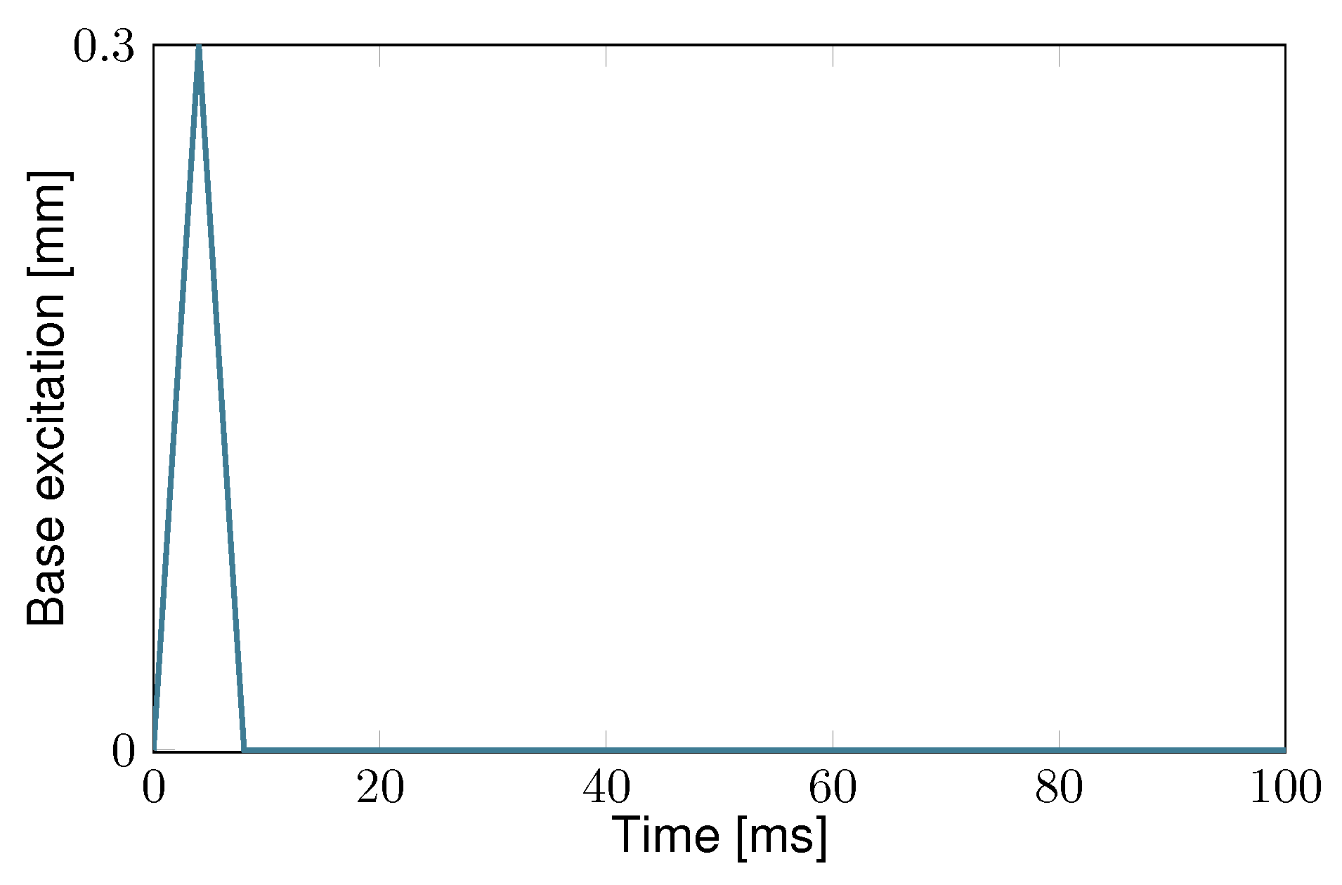
This contribution addresses the numerical optimization of a PEH consisting of a nonlinear electromechanical structure and a nonlinear electric circuit under triangular shock-like excitation. No simplifications are introduced due to the optimization method and arbitrary PEHs can be optimized. Firstly, an implicit coupling between a finite element method (FEM) simulation and an electronic circuit simulator (ECS), recently introduced by the authors in Hegendörfer et al. [13], is used for the analysis of arbitrary PEHs and the optimization problem is presented. Performing multiple simulations to evaluate the objective function is computationally expensive. Hence, a more efficient deep neural network (DNN) is trained based on a set of training data generated from the coupled FEM-ECS simulations. A genetic algorithm then uses the trained DNN to determine the optimal parameters of the PEH that maximize the harvested energy, accounting for a nonlinear stress constraint.

2. Accurate System Simulations of the PEH

In the following, an implicit coupling between an in-house C++ FEM code based on the open source FE library deal.ii [14] and the circuit simulator Matlab/Simulink Simscape is presented. In the approach, recently introduced by authors in Hegendörfer et al. [13], the full capabilities of the FEM can be exploited for the simulation of the electromechanical structure. Nonlinearities and changing boundary conditions can be considered. In addition, an ECS is applied to simulate electric circuits with nonideal components such as diodes. An efficient implicit coupling algorithm based on Newton’s method ensures convergence between the FEM and ECS simulations in each time step.

In the following, the FEM and ECS frameworks and the coupling between them are shortly introduced. More detailed information can be found in Hegendörfer et al. [13].

2.1. FEM Simulation

For the simulation of the electromechanical structure a FEM framework is applied, which we presented in [15]. A nonlinear piezoelectric constitutive law is used to allow for large base excitations. In this case, nonlinear elasticity becomes important and must be considered in the simulations [8]. In Stanton et al. [8] the additional parameters $c_4$ and $c_6$ are postulated for a 1D material model for PZT-5A to include nonlinear elastic behavior via a polynomial function. In Hegendörfer et al. [15] this nonlinear elasticity model is extended to enable 3D FEM simulations and yields

$$\begin{array}{cc}\hfill T_{ij}& =c_{ijkl}^E{S}_{kl}-e_{kij}{E}_k+c_4{\left[S_{mn}{A}_{mn}\right]}^3{A}_{ij}+c_6{\left[S_{mn}{A}_{mn}\right]}^5{A}_{ij}\hfill \\ \hfill D_i& =e_{ikl}{S}_{kl}+{\epsilon }_{ij}^S{E}_j\hfill \end{array}$$

(1)

with the structural tensor $A_{ij}=a_i{a}_j$ and the vector $a_i=e_{1i}$ being equal to the Cartesian basis vector and denoting the direction with the nonlinear elastic behavior. The piezoelectric constitutive law relates the mechanical stresses $T_{ij}$ and the dielectric displacements $D_i$ with the mechanical strain $S_{ij}$ and the electric field $E_i$. Here, $c_{ijkl}^E$ are the components of the elasticity tensor at constant electric field and ${\epsilon }_{ij}^S$ is the dielectric constant at constant strain. The mechanical and electrical fields are coupled via the piezoelectric coupling tensor $e_{kij}$. These constitutive equations are introduced into the balance of linear momentum (for the mechanical problem) and Gauss’ law (for the electro-static problem) and solved with the finite element method.

Ultimately, after applying the FEM for the piezoelectric problem and the Bossak–Newmark method [16] for direct time integration, the nonlinear vector-valued equation to be solved results in

$${\mathit{r}}_{n+1}=\left[1+\alpha \right]{\mathit{f}}_{n+1}^{dyn}-\alpha {\mathit{f}}_n^{dyn}+{\mathit{f}}_{n+1}^{damp}+{\mathit{f}}_{n+1}^{int}-{\mathit{f}}_{n+1}^{ext}=\mathbf{0}$$

(2)

whereby ${\mathit{r}}_{n+1}$ is the residuum at time $t_{n+1}$, n corresponds to the current time step, while $n+1$ denotes the next time step to be computed and $\alpha$ is the Bossak–Newmark parameter. The force vectors contain the mechanical and electrical fields, whereby ${\mathit{f}}^{dyn}$ is the inertial force vector, ${\mathit{f}}^{damp}$ is the damping force vector, ${\mathit{f}}^{int}$ is the vector of internal forces and ${\mathit{f}}^{ext}$ is the vector of external forces. The force vectors are specified in Appendix A, Equations (A1)–(A4). In each time step the system of Equation (2) is solved with the Newton–Raphson method.

To enable efficient FEM time domain simulations, the time step size must be adapted to the current conditions in the simulation. This adaptive time step control is performed with an empirical method presented in Hibbitt and Karlsson [17], which is based on the limitation of a residual calculated between two FEM time steps.

2.2. ECS Simulation

An ECS is a powerful numerical tool for the analysis of arbitrary electric circuits. Generally, an ECS automatically formulates the electric circuit equations by applying Kirchhoff’s circuit laws, and, then, a time integration scheme to solve the obtained equations. In this contribution, the commercial software Matlab/Simulink Simscape is used for the electric circuit simulation.

In the numerical examples, electric circuits with diodes will be considered. These nonlinear electric components are modeled using the Shockley equation

$$i_D=I_S^D\left[e^{\frac{v_D}{n{V}_T}}-1\right]$$

(3)

as in Leadenham and Erturk [7]. Thereby, $v_D$ is the voltage across the diode, $i_D$ is the current flowing through the diode, n is the ideality factor and $V_T$ represents the thermal voltage. Here, $I_S^D$ is a small saturation current, which will flow in reverse direction when a large reverse voltage is applied. Every real diode has a reverse breakdown voltage at which a large current will flow in reverse direction. However, this effect is neglected in the Shockley diode model and, consequently, it is assumed that no breakdown occurs.

2.3. FEM-ECS Coupling

In Hegendörfer et al. [13] an implicit coupling between a 3D FEM simulation of the electromechanical structure and an ECS analysis of the electric circuit is introduced. This coupling method in its voltage controlled form is also used in this contribution and is summarized in the following.

The equilibrium between the FEM and ECS simulations is iteratively obtained at each time step. The relevant variables for the FEM-ECS coupling are the electrode voltage ${\phi }_{el}$ and the electric current ${\dot{Q}}_{el}$ leaving the electrode. These values are influenced on the one hand by the electromechanical structure and on the other hand by the electric circuit. The equilibrium of these values, used in the FEM simulation and the ECS, has to be ensured in each time step. The Newton–Raphson method is applied to iteratively solve this nonlinear coupling equation. Due to the coupling method, there are no constraints on nonlinearities that can be taken in to account in the FEM simulation or the ECS. Here, the system simulation method is used to couple the FEM library deal.ii with the Matlab/Simulink ECS. However, the method is not restricted to any specific software but can be applied to all FEM and ECS tools that can read and export time step results. A detailed description of this implicit coupling method is given in Hegendörfer et al. [13].

3. Definition of the Optimization Problem

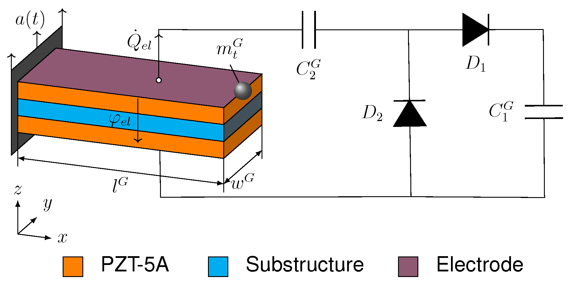
In the following optimization problems, PEHs are considered that consist of a bimorph cantilever beam and either a Greinacher circuit or a standard electric circuit. A prescribed shock-like excitation is applied to the bimorph. The objective of the optimization problem is to evaluate the optimal design variables of the PEH such that the harvested energy is optimized. The PEH with the Greinacher circuit is shown in Figure 1 and that with the standard circuit in Figure 2. The triangular shock-like excitation is illustrated in Figure 3.

The bimorph cantilever beam consists of two layers of PZT-5A, bracketing a passive substructure layer [18]. The layers are poled in opposite directions and connected in series. The thickness of the layers is $0.26$ mm, that of the substructure $0.14$ mm. These geometric parameters are fixed in the optimization. The lenght and the width of the beam can be changed in the optimization, with the constraint that the PZT-5A volume remains constant. Therefore, the length is chosen as a design variable. A tip mass is added to the cantilever beam to ensure a more uniform stress distribution. In the simulation, this tip mass is modeled as a point mass. Its value $m_t$ is used as a design variable in the optimization.

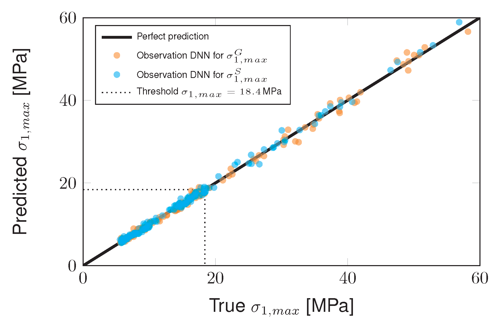
Since PZT-5A is a brittle material it is necessary to ensure that the stresses in the structure do not exceed the strength of the material. The dynamic tensile strength of PZT-5A was reported as 27.6 MPa in Berlincourt et al. [19]. Applying a safety factor of 1.5, a constraint on the maximum principle stress ${\sigma }_1$ of ${\sigma }_1\le 18.4$ MPa is used in the optimization.

Since the electromechanical structure operates in its resonance frequency, mechanical damping significantly influences its behavior. The damping caused by the electric circuit is accurately considered in the system simulations. Other sources of damping, e.g. material damping or support damping, are modeled by means of a Rayleigh type damping, compare Equation (A4). This simplified model assumes that the damping of the structure is mass and stiffness proportional. The two Rayleigh coefficients, ${\alpha }_R$ and ${\beta }_R$, see Equation (A4), have to be determined experimentally for each particular structure. During the optimization process, the geometry of the electromechanical structure changes and therefore, the Rayleigh coefficients have to be adjusted. To achieve comparable damping in all configurations, the Rayleigh coefficients are adapted in a way that the damping ratio of the first vibration mode ${\zeta }_1$ is constant. This damping ratio can be computed by means of the Rayleigh coefficients as

$${\zeta }_1=\frac{{\alpha }_R}{2{\omega }_1}+\frac{{\beta }_R{\omega }_1}{2}$$

(4)

and was experimentally measured for the original bimorph structure in Erturk and Inman [18] as ${\zeta }_1$ = 0.027. This constant damping ratio is ensured for all bimorph configurations in the simulations by keeping ${\beta }_R=5·{10}^{-5}$ s/rad fix and computing ${\alpha }_R$ from Equation (4), for ${\zeta }_1=0.027$ and the first short-circuit eigenfrequency of the particular configuration ${\omega }_1$.

The bimorph electromechanical structure is connected to two different circuits namely the Greinacher [20,21] and standard circuit. Figure 1 shows the electromechanical structure coupled to the Greinacher circuit, which consists of two diodes and two capacitors whose capacitance values $C_1^G$ and $C_2^G$ are defined as design variables for the optimization. The harvested energy $\mathcal{E}\left(\mathcal{X}\right)$ is stored in the capacitor $C_1^G$ and the voltage across $C_1^G$ is denoted as $V_{C_1}^G$. 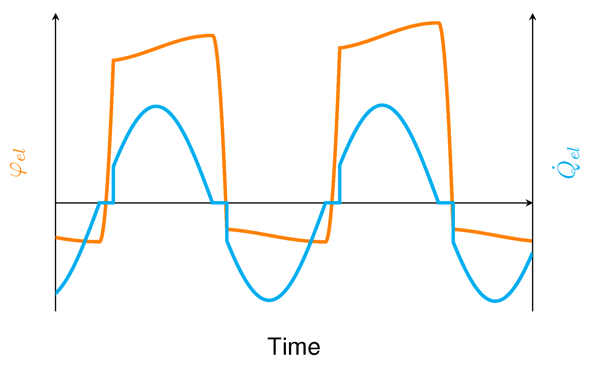Figure 4 presents the typical wave form of the electric voltage and the current on the electrode for the Greinacher circuit under harmonic base excitation of the electromechanical structure. Because the polarity of the electric current charging capacitor $C_2^G$ changes during operation of the circuit, the voltage across capacitor $C_2^G$ also changes its direction. Since the direction of the voltage $V_{C_1}^G$ across capacitor $C_1^G$ is different than that across $C_2^G$ when the electric voltage ${\phi }_{el}$ increases, the electric voltage value ${\phi }_{el}$ necessary to charge capacitor $C_1^G$ is reduced. Only one diode is used when charging the capacitor $C_1^G$, resulting in relatively low electrical losses.

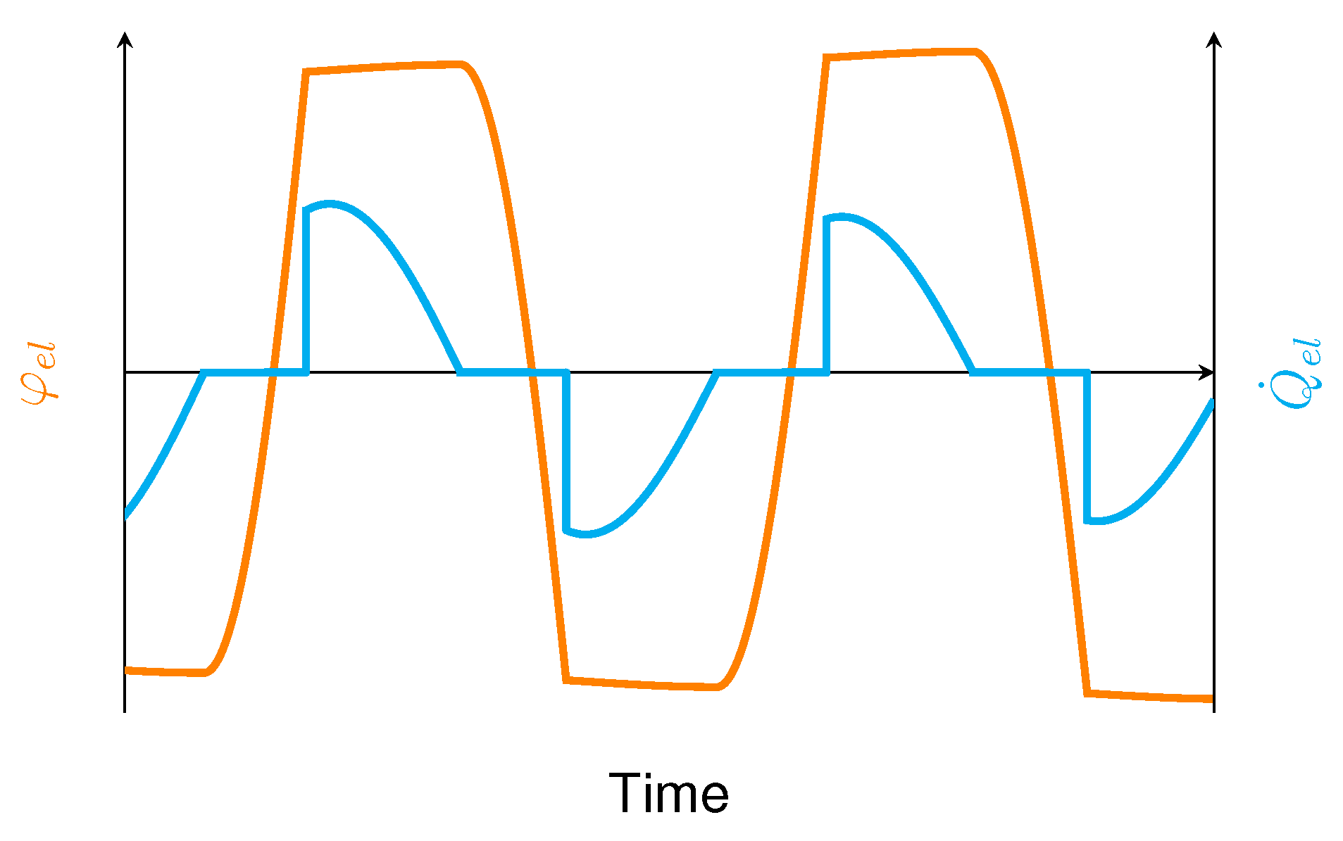
Figure 2 presents the electromechanical structure equipped with the standard circuit. It consists of four diodes forming a full bridge rectifier and a storage capacitor, whose capacitance value $C_1^S$ is to be optimized. In Figure 5 the typical wave form of the electrode voltage and the electric current for the standard circuit under harmonic base excitation of the electromechanical structure is shown. During charging, the voltage $V_{C_1}^S$ across $C_1^S$ increases and, thus higher electrode voltages $|{\phi }_{el}|$ are necessary to further charge the capacitor $C_1^S$. The performance of the standard circuit does not depend on the polarity of the electrode voltage ${\phi }_{el}$ resulting in symmetric wave forms for the electrical signals. When the capacitor $C_1^S$ is charged, the electric current ${\dot{Q}}_{el}$ has to pass two diodes, which leads to higher electric losses compared to the Greinacher circuit.

For the electromechanical structure with the Greinacher circuit, there are four design variables ${\mathcal{X}}^G$ in the optimization problem, the length of the beam $l^G$, the tip mass $m_t^G$ and the two capacitances $C_1^G$ and $C_2^G$. Their lower and upper bounds are given in

Table 1. Design variables ${\mathcal{X}}^G$ with lower and upper bounds for the configuration with Greinacher circuit.

Design Variables ${\mathcal{X}}^{\mathcal{G}}$	${\mathcal{X}}_{\mathit{min}}^{\mathit{G}}$	${\mathcal{X}}_{\mathit{max}}^{\mathit{G}}$
length $l^G$	40 mm	80 mm
tip mass $m_t^G$	5 g	15 g
capacitance $C_1^G$	0 µF	1 µF
capacitance $C_2^G$	0 µF	8 µF

. The electromechanical structure with the standard circuit has three design variables ${\mathcal{X}}^S$, length of the beam $l^S$, tip mass $m_t^S$ and the capacitance $C_1^S$. Their bounds are given in

Table 2. Design variables ${\mathcal{X}}^S$ with lower and upper bounds for the configuration with standard circuit.

Design Variables ${\mathcal{X}}^{\mathcal{S}}$	${\mathcal{X}}_{\mathit{min}}^{\mathit{S}}$	${\mathcal{X}}_{\mathit{max}}^{\mathit{S}}$
length $l^S$	40 mm	80 mm
tip mass $m_t^S$	5 g	15 g
capacitance $C_1^S$	0 µF	1 µF

.

The optimization problem to maximize the harvested energy reads

$$\begin{array}{cc}\hfill max\mathcal{E}& \left(\mathcal{X}\right)\hfill \\ \hfill \mathrm{s}.\mathrm{t}.{\sigma }_{1,max}\left(\mathcal{X}\right)& \le 18.4\mathrm{MPa}\hfill \\ \hfill {\mathcal{X}}_{min}\le & {\mathcal{X}}_i\le {\mathcal{X}}_{max}\hfill \end{array}$$

(5)

whereby the maximum stress constraint and the bounds for the design variables have to be taken in to account. The harvested energy $\mathcal{E}\left(\mathcal{X}\right)$ is stored in the capacitor $C_1$ and can be obtained as

$$\mathcal{E}\left(\mathcal{X}\right)=\frac{1}{2}{C}_1{V_{C_1}\left(\mathcal{X}\right)}^2$$

(6)

whereby $V_{C_1}$ is the voltage across the capacitor $C_1$ and depends on the design variables $\mathcal{X}$.

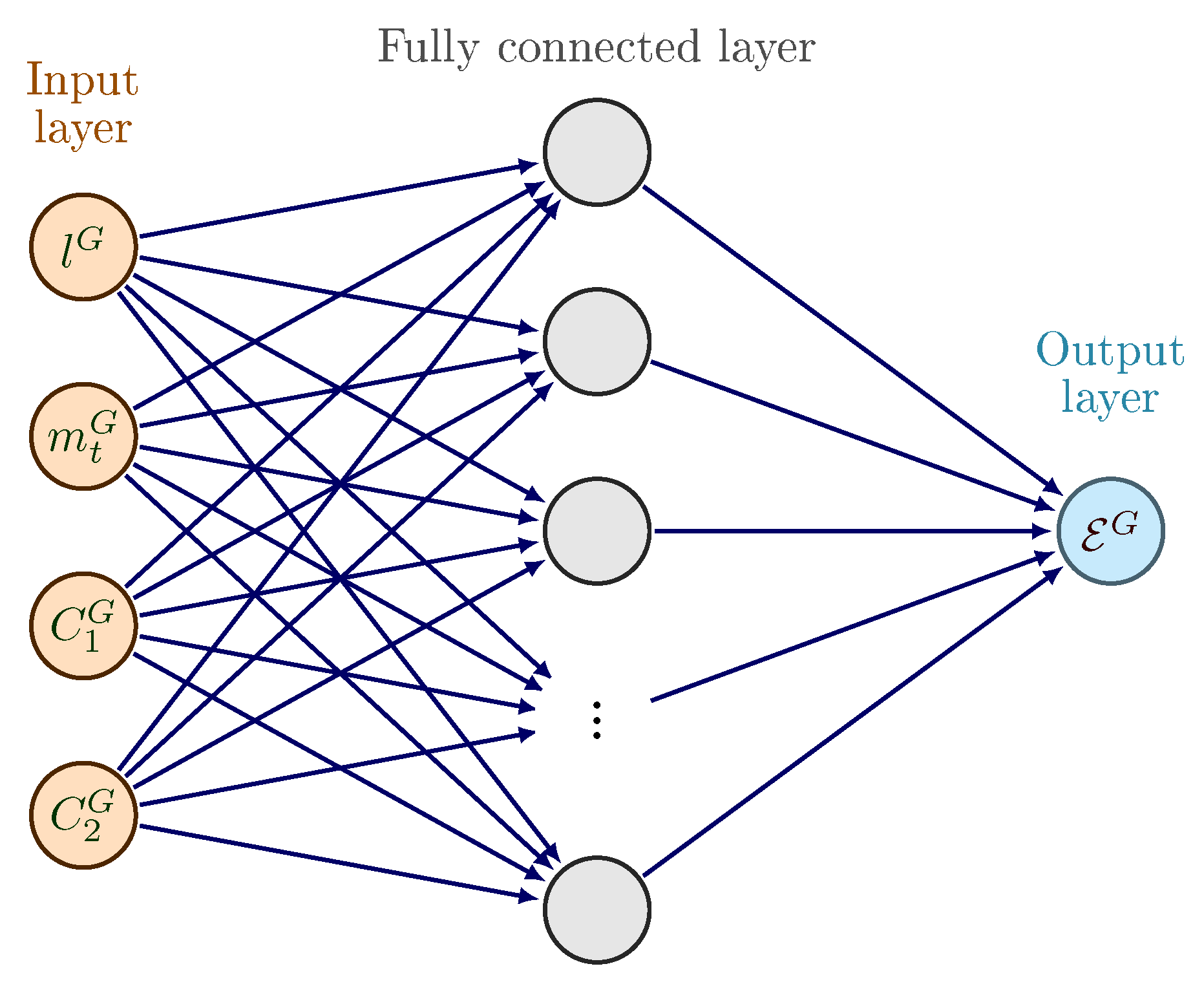
The solution of the optimization problem (5) usually requires the solution of the system simulation and the computation of the harvested energy $\mathcal{E}\left(\mathcal{X}\right)$ for many combinations of the design variables. Since the system simulations are quite expensive, a deep neural network is trained to compute the harvested energy and the maximum principle stress depending on the design variables. After the training phase, this DNN model can then efficiently be evaluated during the solution of optimization problem (5).

4. DNN Models to Approximates the System Simulations

In the presented optimization problem (5), the harvested energy $\mathcal{E}$ and the maximum mechanical stress ${\sigma }_{1,max}$ must be evaluated for a given set of design variables $\mathcal{X}$. Two separate DNN models are derived for this task, both, the Greinacher and the standard circuit configurations. Thus, four different DNNs are deduced, two for the Greinacher circuit configuration (for ${\mathcal{E}}^G$ and ${\sigma }_{1,max}^G$) and two for the standard circuit (for ${\mathcal{E}}^S$ and ${\sigma }_{1,max}^S$). In the following, the generation of training data for the DNNs and the training process itself are described and the performance of the DNNs is evaluated.

4.1. Generation of Training Data

Training data are essential for the learning process of a DNN to adjust its internal parameters. The accuracy of the DNNs improves with the amount of training data. Here, for the configurations with the Greinacher and standard circuit, 800 randomly selected sets of design variables $\mathcal{X}$ are defined in each case. Subsequently, the coupled FEM-ECS simulation framework is used to evaluate the harvested energy $\mathcal{E}$ and the maximum mechanical stress ${\sigma }_{1,max}$. For each set of design variables $\mathcal{X}$, one time domain system simulation run is required.

The coupled FEM-ECS simulations are quite expensive. To reduce the computational costs, an adaptive time stepping scheme is applied, as described in Section 2.1. Furthermore, a termination criterion for the simulations is introduced. Due to the triangular shock-like excitation, energy is only harvested during a certain period of time, which depends on the particular design variables. When no energy is harvested anymore for longer than 1.3 times the period of oscillation, the simulation is stopped.

The bimorph electromechanical structure is discretized with 90 quadratic hexahedral elements. A Young’s modulus of 105 GPa is used for the substructure and the material parameters for PZT-5A are listed in the Appendix B in Equations (A7)–(A9). For the ECS analysis in Matlab/Simulink, the daessc solver is used with an automatic choice of minimum and maximum time step sizes (setting auto). The specified values for the diode parameters in Equation (3) are listed in the Appendix C. Using one Intel Core i7-9700, one system simulation with the coupled FEM-ECS approach to evaluate the harvested energy $\mathcal{E}$ and the maximum mechanical stress ${\sigma }_{1,max}$ takes about 25 min.

4.2. Training of the DNNs

To efficiently predict the harvested energy $\mathcal{E}$ and the maximum mechanical stress ${\sigma }_{1,max}$ two DNNs are used for the each of the two configurations. All DNNs applied in the present work share a similar structure, consisting of an input layer, one fully connected layer and an output layer. The input layers for the DNNs for the Greinacher circuit configuration consist of four neurons, each for one design variable. Consequently, only three neurons are necessary for the input layer of the two DNNs for the standard circuit configuration. Subsequently, a fully connected layer is used, where all neurons of this layer are connected to all neurons of the input layer [22]. For all DNNs a constant number of 100 neurons in the fully connected layer is chosen. However, this number can be selected freely and independently for each DNN, but good accuracy was observed for 100 neurons. The output layer of each DNN contains only one neuron representing either the harvested energy $\mathcal{E}$ or the maximum mechanical stress ${\sigma }_{1,max}$ for the two configurations. Figure 6 presents the structure of the DNN predicting the harvested energy ${\mathcal{E}}^G$ for the configuration with Greinacher circuit.

The two datasets containing 800 data points for each configuration were randomly partitioned into a test set containing 160 data points (20%) and a training set containing 640 data points (80%). The training sets are used to optimize the internal parameters of the DNNs and the test sets to evaluate the accuracy of the resulting DNNs. This training process was performed using the Matlab Regression Learner app [22]. In the following, the accuracy of the DNNs is assessed.

4.3. Performance Evaluation of the DNNs

The trained DNNs are used to predict data points from the test set. Then, the predictions are compared to the true values from the test set to evaluate the accuracy of the DNNs. Figure 7 presents the comparison between the predictions of the DNNs and the true values for the harvested energies of the Greinacher circuit configuration ${\mathcal{E}}^G$ and of the standard circuit configuration ${\mathcal{E}}^S$. The black line represents the perfect accuracy, as the the DNN predictions agree with the true values. A high accuracy of the two DNNs can be observed. This is confirmed by the low root mean squared errors (RMSE) and normalized root mean squared errors (NRMSE) for the DNNs for the harvested energies for both electric circuits

$$\begin{array}{ccc}\hfill RMSE\left({\mathcal{E}}^G\right)=0.73\mathsf{\mu }\mathrm{J}& \mathrm{and}NRMSE\left({\mathcal{E}}^G\right)=\hfill & \hfill 0.06\\ \hfill RMSE\left({\mathcal{E}}^S\right)=0.69\mathsf{\mu }\mathrm{J}& \mathrm{and}NRMSE\left({\mathcal{E}}^S\right)=\hfill & \hfill 0.05\end{array}$$

(7)

with

$$RMSE\left(Y\right)=\sqrt{\frac{1}{n}\sum _{i=1}^n{\left[Y_i-{\widehat{Y}}_i\right]}^2}$$

(8)

and

$$NRMSE\left(Y\right)=\frac{nRMSE\left(Y\right)}{{\sum }_{i=1}^n{Y}_i}$$

(9)

where n is the number of data points, $Y_i$ are the true values and ${\widehat{Y}}_i$ are the DNN predictions.

Figure 8 compares the predictions of the DNNs of the maximum mechanical stress for the configurations with Greinacher ${\sigma }_{1,max}^G$ and standard circuit ${\sigma }_{1,max}^S$ against the true values from the coupled FEM-ECS simulations. A good agreement can also be observed for both electric circuits

$$\begin{array}{ccc}\hfill RMSE\left({\sigma }_{1,max}^G\right)=0.80\mathrm{MPa}& \mathrm{and}NRMSE\left({\sigma }_{1,max}^G\right)=\hfill & \hfill 0.05\\ \hfill RMSE\left({\sigma }_{1,max}^S\right)=0.62\mathrm{MPa}& \mathrm{and}NRMSE\left({\sigma }_{1,max}^S\right)=\hfill & \hfill 0.04\end{array}$$

(10)

Overall, as the comparisons with the test sets show, the predictions of the trained DNNs are very accurate. One evaluation of a DNN requires approximately $0.003$ s, which is around $5\times {10}^5$ times faster than one evaluation with the coupled time domain FEM-ECS simulation framework. Therefore, the trained DNNs enable the solution and analysis of the optimization problem (5).

5. Optimization Results

A genetic algorithm is used to solve the optimization problem (5) and to find the optimal set of design variables for the configuration with Greinacher circuit ${\widehat{\mathcal{X}}}^G$ and for the configuration with standard circuit ${\widehat{\mathcal{X}}}^S$. Genetic algorithms in combination with DNNs have been shown to be effective for comparable optimization problems in Bagheri et al. [6], Chimeh et al. [23], Nabavi and Zhang [24]. The idea of a genetic algorithm is to repeatedly modify a population of individual solutions by using them as parents to produce the children of the next generation. Over several generations, the population evolves towards an optimal solution [22]. Genetic algorithms usually need a high number of objective function evaluations, but these are very inexpensive due to the use of DNNs.

Table 3. Optimal values for the design variables for the Greinacher configuration ${\widehat{\mathcal{X}}}^G$ and for the standard circuit configuration ${\widehat{\mathcal{X}}}^S$.

${\widehat{\mathcal{X}}}^{\mathit{G}}$	${\widehat{\mathcal{X}}}^{\mathit{S}}$
${\widehat{l}}^G=48.46$ mm	${\widehat{l}}^S=47.64$ mm
${\widehat{m}}_t^G=10.83$ g	${\widehat{m}}_t^S=12.91$ g
${\widehat{C}}_1^G=0.19$ µF	${\widehat{C}}_1^S=0.60$ µF
${\widehat{C}}_2^G=5.79$ µF	-

presents the optimal values for the design variables for the configuration with Greinacher circuit ${\widehat{\mathcal{X}}}^G$ and for the configuration with standard circuit ${\widehat{\mathcal{X}}}^S$.

To obtain the optimal values $\widehat{\mathcal{X}}$, the genetic algorithm requires around $8.5\times {10}^4$ evaluations of the harvested energy ${\mathcal{E}}^G$ for the Greinacher configuration and around $6.0\times {10}^4$ evaluations of ${\mathcal{E}}^S$ for the standard circuit configuration since it has one design variable less.

The PEHs with these optimal design variables are simulated with the coupled FEM-ECS simulation method.

Table 4. Comparison between the results for the optimal design varaibles $\widehat{\mathcal{X}}$ of the DNNs against that of the FEM-ECS coupling for the harvested energy $\widehat{\mathcal{E}}$ and the maximum mechanical stress ${\widehat{\sigma }}_{1,max}$.

Quantity	DNNs ($\widehat{\mathcal{X}}$)	FEM-ECS ($\widehat{\mathcal{X}}$)	Rel. Error	Abs. Error
${\widehat{\mathcal{E}}}^G$	24.8 µJ	24.1 µJ	2.9%	0.7 µJ
${\widehat{\sigma }}_{1,max}^G$	18.4 MPa	19.1 MPa	3.7%	0.7 MPa
${\widehat{\mathcal{E}}}^S$	26.0 µJ	24.8 µJ	4.8%	1.2 µJ
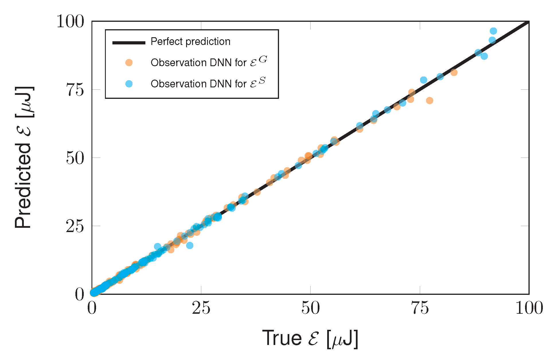
${\widehat{\sigma }}_{1,max}^S$	18.4 MPa	18.2 MPa	1.1%	0.2 MPa

compares the predicted values of the DNNs for the maximum harvested energy $\widehat{\mathcal{E}}$ and the maximum mechanical stress ${\widehat{\sigma }}_{1,max}$ for the optimal design variables $\widehat{\mathcal{X}}$ against the true values obtained by the coupled FEM-ECS simulations. The relative error is below 5% for the predictions of the DNNs for both configurations, confirming the accuracy of the DNNs.

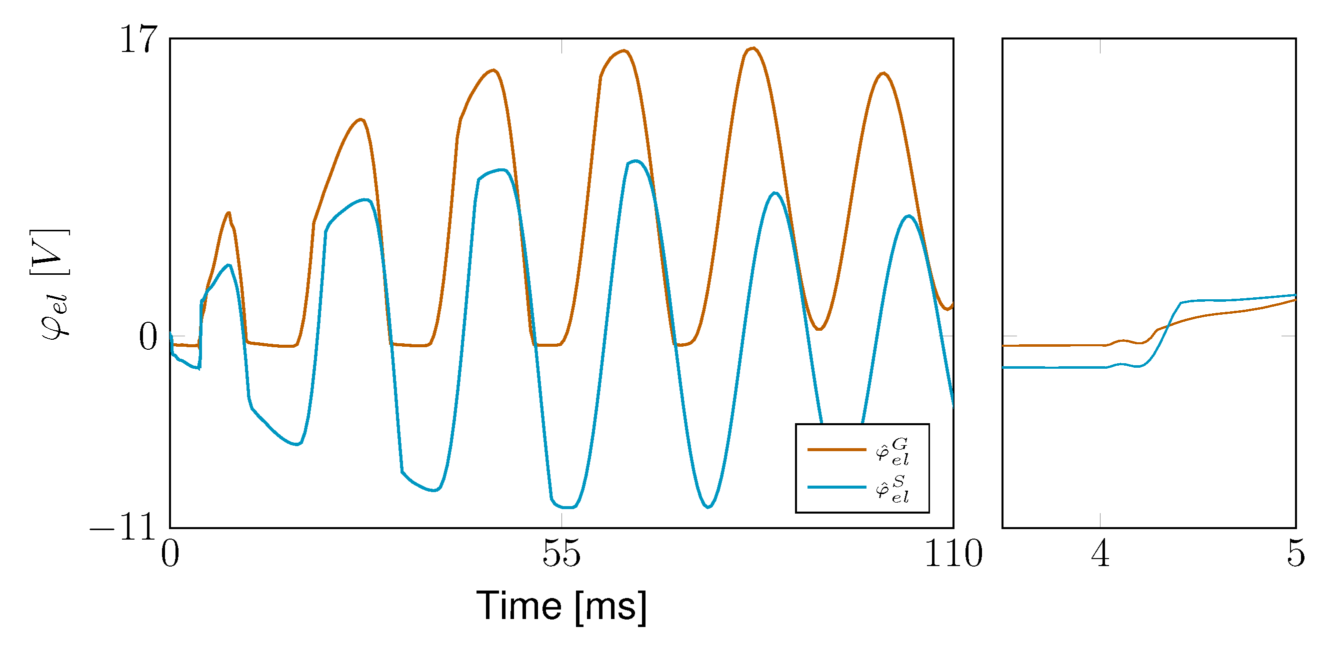
Figure 9 shows the time signals of the electrode voltage for the Greinacher configuration ${\widehat{\phi }}_{el}^G$ and for the standard circuit configuration ${\widehat{\phi }}_{el}^S$ obtained by the coupled FEM-ECS simulations. In the beginning of the simulation, the electromechanical structure is at rest and the base excitation starts. The shock-like base excitations results in higher frequency modes, which can be observed in the zoom-in in Figure 9 on the right. Because the capacitor ${\widehat{C}}_2^G$ of the optimal Greinacher configuration is relatively large, the electric voltage ${\widehat{\phi }}_{el}^G$ can not reach high negative values. As a result, the oscillation of the electric voltage ${\widehat{\phi }}_{el}^G$ is shifted into the positive range. Consequently, the storage capacitor ${\widehat{C}}_1^G$ of the optimal Greinacher configuration is much smaller compared to that of the optimal standard circuit configuration ${\widehat{C}}_1^S$ and the electric voltage ${\widehat{\phi }}_{el}^G$ becomes significantly higher than ${\widehat{\phi }}_{el}^S$. After around 82 ms for the Greinacher configuration and at around 66 ms for the standard circuit configuration the electric voltage ${\widehat{\phi }}_{el}$ can not reach sufficiently high values anymore to charge the storage capacitor ${\widehat{C}}_1$. Due to the damping, the oscillation of the electrode voltage ${\widehat{\phi }}_{el}$ then decays.

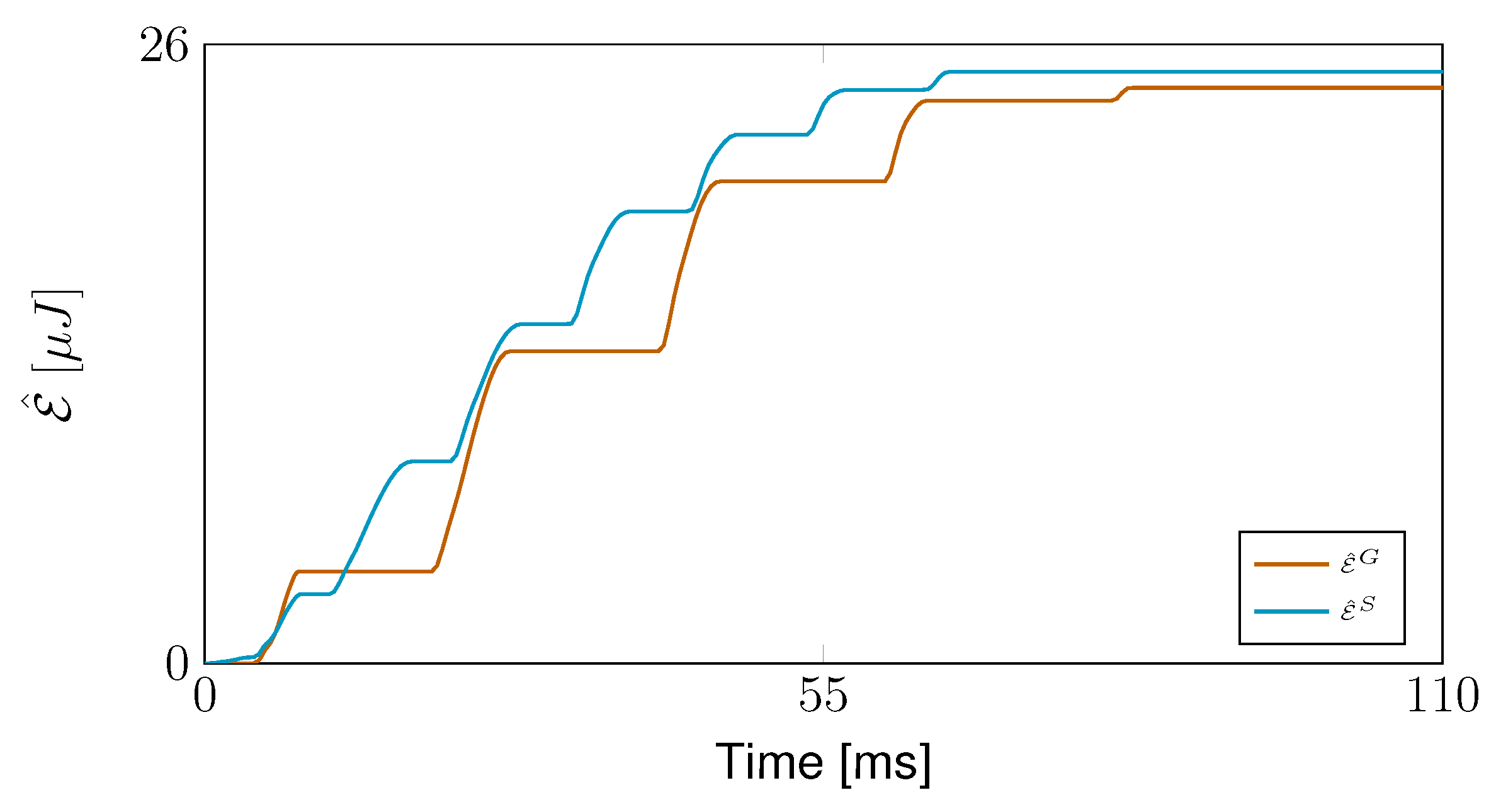
Figure 10 presents the time signals of the maximum harvested energy for the Greinacher ${\widehat{\mathcal{E}}}^G$ and for the standard circuit configuration ${\widehat{\mathcal{E}}}^S$ obtained by the coupled FEM-ECS simulations. At the beginning of the simulations, no energy is stored in the storage capacitor $C_1$ and the harvested energy $\widehat{\mathcal{E}}$ vanishes. When the electromechanical structure oscillates, the standard circuit can harvest energy at positive and negative electrode voltages ${\phi }_{el}$. In contrast, the Greinacher circuit can only harvest energy at positive electrode voltage ${\phi }_{el}$. Therefore, the harvested energy of the standard circuit increases more uniformly compared to the Greinacher circuit. However, the total harvested energy is similar for both configurations.

6. Discussion of the Results

The computational efficiency of DNNs allows for an extended analysis of the optimization problem. The relations between several design variables were examined in detail and resulted in the following observations:

• The maximum harvested energies are obtained for configurations that result in maximum principle stresses close to the constraint value.
• The capacitances of the electric circuits have a strong influence on the optimal length and tip mass of the beam.
• For the Greinacher circuit, the optimal design does not depend on capacitance $C_2^G$.

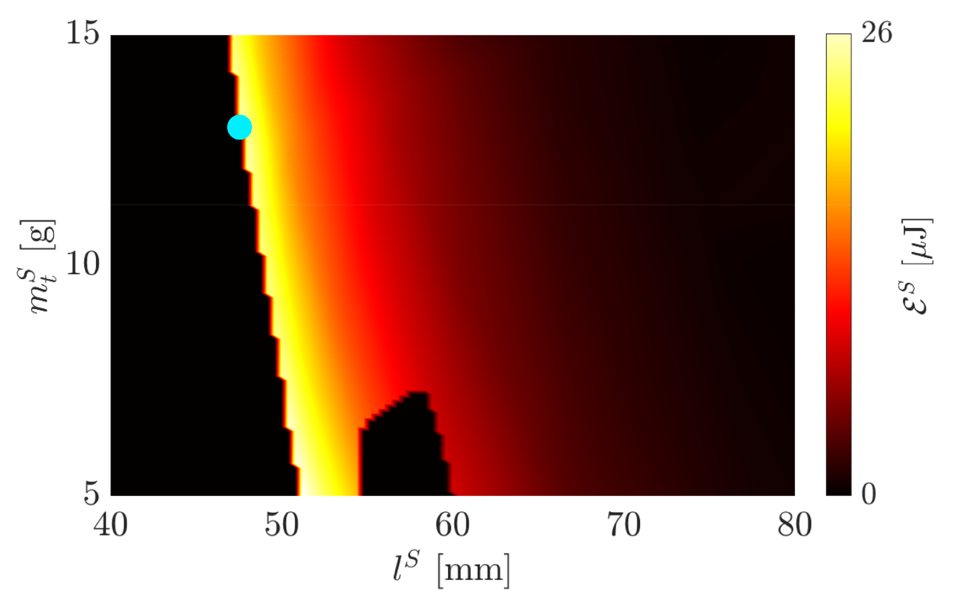
To illustrate the first finding, Figure 11 presents the harvested energy for the standard circuit configuration ${\mathcal{E}}^S$ when the tip mass $m_t^S$ and beam length $l^S$ are varied, with the capacitor ${\widehat{C}}_1^S=0.60$ µF set to the optimal value. Combinations of $m_t^S$ and $l^S$ that cause violations of the nonlinear stress constraint in Equation (5) are assigned 0 µJ of harvested energy since failure of the electromechanical structure is assumed. A clear demarcation between parameter combinations with admissible and non-admissible stresses is visible. All parameter combinations along this line give high values for the harvested energy ${\mathcal{E}}_S$ since larger mechanical stresses result in higher harvested energies due to the piezoelectric effect. The energy values along this line are so close that various optimal parameter combinations of $m_t^S$ and $l^S$ are possible, taking into account the accuracy of the DNNs.

There is also a limited region for a small tip mass and a length of 55–60 mm, in which the stress constraint is violated. The maximum stress ${\sigma }_{1,max}$ in this region is slightly higher than the maximum value of 18.4 MPa, which is also confirmed by the coupled FEM-ECS simulations. This slight increase in the stresses can be caused by an unfavorable deformation response of the electromechanical structure, influenced by the capacitance and the nonlinear piezoelectric material law. For the PEH with the Greinacher circuit, the harvested energy plotted over $l^G$ and $m_t^G$ looks very similar. These results affirm the importance of an optimization procedure including a stress constraint for the piezoelectric material. Due to the piezoelectric effect, high amounts of energy are harvested for high stresses in the material. Therefore, evaluation of a stress constraint during the optimization is required to ensure that the PEH does not only harvest the highest amount of energy but can also withstand the mechanical stresses that occur.

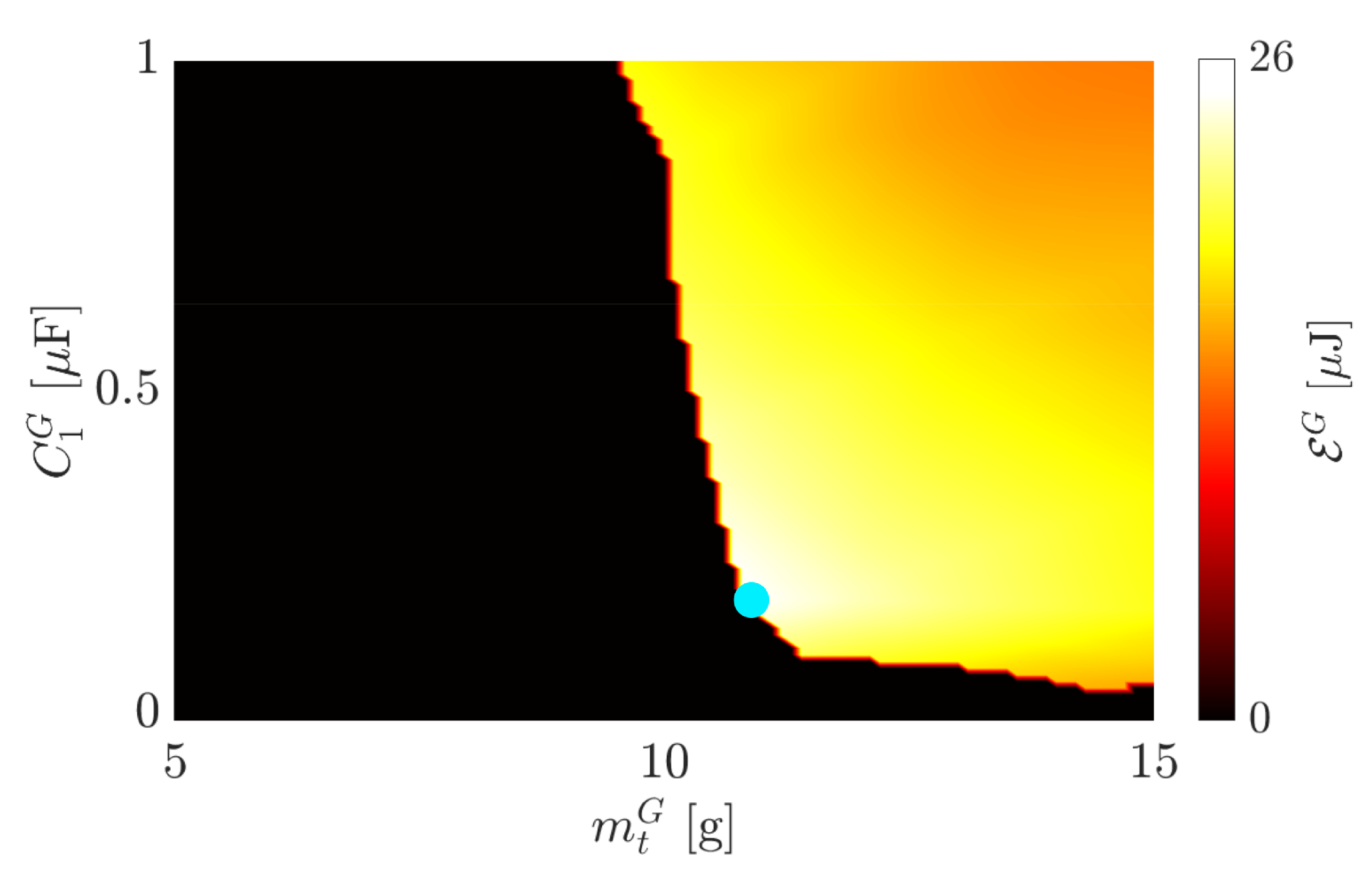
Figure 12 presents the harvested energy for the Greinacher circuit configuration ${\mathcal{E}}^G$ when the tip mass $m_t^G$ and capacitor $C_1^G$ are varied, with the length ${\widehat{l}}^G=48.46$ mm and capacitor ${\widehat{C}}_2^G=5.79$ µF set to their optimal values. When the stress constraint is violated, 0 µJ of harvested energy is assigned. The optimal combination of $m_t^G$ and $C_1^G$ is at the border defined by the stress constraints. Due to the coupling between the electromechanical structure and the electric circuit, both the tip mass $m_t$ and the storage capacitor $C_1^G$ significantly influence the mechanical stresses, resulting in a curved boundary of admissible stresses. The harvested energy for the standard circuit plotted over the mass $m_t^S$ and the capacitance $C_1^S$ looks similar, only that the optimum is obtained for larger values for $C_1^G$. The energy curves over the capacitance and the beam length also show similar characteristics. It is important to note that the capacitance significantly influences the optimal mass and length values and also the position of the stress constraint boundary. It is therefore clear that the simultaneous optimization of the electromechanical structure and the electric circuit is necessary.

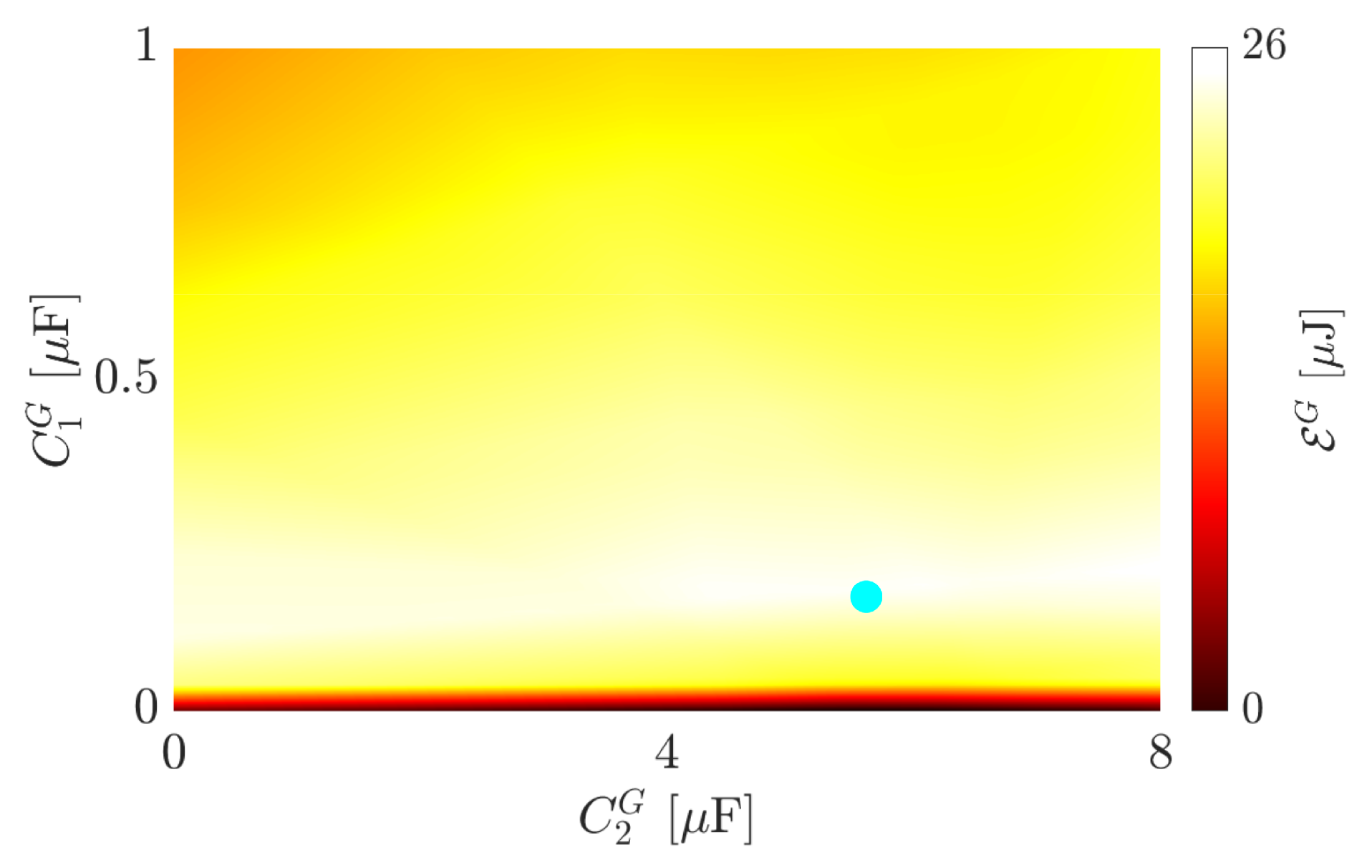
Figure 13 shows the harvested energy for the Greinacher circuit configuration ${\mathcal{E}}^G$ for different capacitors $C_1^G$ and $C_2^G$ while the length ${\widehat{l}}^G=48.46$ mm and the tip mass ${\widehat{m}}_t^G=10.83$ g are set to their optimal values. The capacitor $C_1^G$ has a significant influence on the harvested energy. In contrast, there is nearly no dependency of the harvested energy on the capacitor $C_2^G$. Therefore, it could be neglected and a half-diode bridge circuit would be obtained. Because significant higher electrode voltages can be reached with the Greinacher circuit than with the standard circuit, the optimal value for the capacitor of the Greinacher circuit $C_1^G$ is much smaller than that of the standard circuit $C_1^S$.

7. Conclusions

This contribution introduces a numerical approach to find optimal design variables for an electrically and mechanically nonlinear PEH taking into account a stress constraint. A single shock event in the form of a triangular shock-like base excitation is considered. A bimorph electromechanical structure equipped with Greinacher or standard circuit is used and various design variables are defined that need to be optimized to obtain the maximum harvested energy. For the system simulation of the PEH an implicit FEM-ECS coupling method is applied. Within the coupled system simulation, the capabilities of the FEM and the ECS can be fully exploited and nonlinear PEH under shock-like excitations can be accurately simulated. However, this highly accurate simulation method is computationally expensive and inappropriate for a large number of simulations as required for the repeated evaluation of the objective function during an optimization procedure. Therefore, the coupled FEM-ECS method is used to generate training data for DNNs that are used afterwards to evaluate the objective function in the optimization procedure. It is shown that the trained DNNs are very computational efficient and able to approximate the behavior of the different PEHs configurations accurately. A genetic algorithm is applied to find optimal design variables that maximize the harvested energy and do not violate the stress constraint.

The optimal configurations of the PEH with the Greinacher and the standard circuit harvest approximately the same amount of energy. The optimal value of the storage capacitor of the Greinacher circuit configuration is much smaller than that of the standard circuit configuration, resulting in a higher capacitor voltage in the Greinacher circuit configuration. In energy harvesting applications, higher voltages are usually preferred because they result in lower electrical losses when the electrical energy in the storage capacitor is further processed. The result that the two circuits harvest approximately the same amount of energy applies only to the optimization problem considered and may change under other conditions, e.g., other base excitations or geometries of the PEH.

For the PEH with both electric circuits the maximum harvested energies occur at the boundary defined by the stress constraint. The position of this boundary in the parameter space depends on the electric circuit parameters. It is shown that the storage capacitor has a significant influence on the admissible tip mass if the stress constraint is not to be violated. For shock-like excitations, the influence of the capacitor $C_2^G$ of the Greinacher circuit on the harvested energy is negligible. Consequently, the capacitor $C_2^G$ can be removed without significant loss of harvested energy and the Greinacher circuit reduces to the half-diode bridge circuit.

In summary, the DNNs, trained by means of accurate coupled FEM-ECS simulations, are able to approximate the behavior of nonlinear PEHs under shock-like excitations. The presented DNN-based numerical optimization procedure can therefore be used to design and optimize general nonlinear PEHs.

References

1. Shirvanimoghaddam, M.; Shirvanimoghaddam, K.; Abolhasani, M.M.; Farhangi, M.; Barsari, V.Z.; Liu, H.; Dohler, M.; Naebe, M. Towards a green and self-powered Internet of Things using piezoelectric energy harvesting. IEEE Access 2019, 7, 94533–94556. [Google Scholar] [CrossRef]
2. Safaei, M.; Sodano, H.A.; Anton, S.R. A review of energy harvesting using piezoelectric materials: State-of-the-art a decade later (2008–2018). Smart Mater. Struct. 2019, 28, 113001. [Google Scholar] [CrossRef]
3. Dietl, J.M.; Garcia, E. Beam shape optimization for power harvesting. J. Intell. Mater. Syst. Struct. 2010, 21, 633–646. [Google Scholar] [CrossRef]
4. Wein, F.; Kaltenbacher, M.; Stingl, M. Topology optimization of a cantilevered piezoelectric energy harvester using stress norm constraints. Struct. Multidiscip. Optim. 2013, 48, 173–185. [Google Scholar] [CrossRef]
5. Miller, L.M.; Elliott, A.D.; Mitcheson, P.D.; Halvorsen, E.; Paprotny, I.; Wright, P.K. Maximum performance of piezoelectric energy harvesters when coupled to interface circuits. IEEE Sens. J. 2016, 16, 4803–4815. [Google Scholar] [CrossRef] [Green Version]
6. Bagheri, S.; Wu, N.; Filizadeh, S. Application of artificial intelligence and evolutionary algorithms in simulation-based optimal design of a piezoelectric energy harvester. Smart Mater. Struct. 2020, 29, 105004. [Google Scholar] [CrossRef]
7. Leadenham, S.; Erturk, A. Mechanically and electrically nonlinear non-ideal piezoelectric energy harvesting framework with experimental validations. Nonlinear Dyn. 2020, 99, 625–641. [Google Scholar] [CrossRef]
8. Stanton, S.C.; Erturk, A.; Mann, B.P.; Dowell, E.H.; Inman, D.J. Nonlinear nonconservative behavior and modeling of piezoelectric energy harvesters including proof mass effects. J. Intell. Mater. Syst. Struct. 2012, 23, 183–199. [Google Scholar] [CrossRef]
9. Stanton, S.C.; Erturk, A.; Mann, B.P.; Inman, D.J. Nonlinear piezoelectricity in electroelastic energy harvesters: Modeling and experimental identification. J. Appl. Phys. 2010, 108, 074903. [Google Scholar] [CrossRef] [Green Version]
10. Gammaitoni, L.; Neri, I.; Vocca, H. Nonlinear oscillators for vibration energy harvesting. Appl. Phys. Lett. 2009, 94, 164102. [Google Scholar] [CrossRef]
11. Cai, W.; Harne, R.L. Vibration energy harvesters with optimized geometry, design, and nonlinearity for robust direct current power delivery. Smart Mater. Struct. 2019, 28, 075040. [Google Scholar] [CrossRef]
12. Zhou, S.; Lallart, M.; Erturk, A. Multistable vibration energy harvesters: Principle, progress, and perspectives. J. Sound Vib. 2022, 116886. [Google Scholar] [CrossRef]
13. Hegendörfer, A.; Steinmann, P.; Mergheim, J. An implicitly coupled finite element—electronic circuit simulator method for efficient system simulations of piezoelectric energy harvesters. J. Intell. Mater. Syst. Struct. 2023, accepted. [Google Scholar]
14. Arndt, D.; Bangerth, W.; Clevenger, T.C.; Davydov, D.; Fehling, M.; Garcia-Sanchez, D.; Harper, G.; Heister, T.; Heltai, L.; Kronbichler, M.; et al. The deal.II library, Version 9.1. J. Numer. Math. 2019, 27, 203–213. [Google Scholar] [CrossRef]
15. Hegendörfer, A.; Steinmann, P.; Mergheim, J. Nonlinear finite element system simulation of piezoelectric vibration-based energy harvesters. J. Intell. Mater. Syst. Struct. 2022, 33, 1292–1307. [Google Scholar] [CrossRef]
16. Wood, W.; Bossak, M.; Zienkiewicz, O. An alpha modification of Newmark’s method. Int. J. Numer. Methods Eng. 1980, 15, 1562–1566. [Google Scholar] [CrossRef]
17. Hibbitt, H.; Karlsson, B. Analysis of Pipe Whip; Technical Report; Hibbitt and Karlsson: RI, USA, 1979; Available online: https://inis.iaea.org/search/search.aspx?orig_q=RN:11538109 (accessed on 19 December 2022).
18. Erturk, A.; Inman, D.J. An experimentally validated bimorph cantilever model for piezoelectric energy harvesting from base excitations. Smart Mater. Struct. 2009, 18, 025009. [Google Scholar] [CrossRef]
19. Berlincourt, D.; Krueger, H.; Near, C. Properties of Morgan Electro Ceramic Ceramics; Technical Publication TP-226; Morgan Electro Ceramics: Cleveland, OH, USA, 2000. [Google Scholar]
20. Qiu, J.; Jiang, H.; Ji, H.; Zhu, K. Comparison between four piezoelectric energy harvesting circuits. Front. Mech. Eng. China 2009, 4, 153–159. [Google Scholar] [CrossRef]
21. Abidin, N.A.K.Z.; Nayan, N.M.; Azizan, M.M.; Ali, A. Analysis of voltage multiplier circuit simulation for rain energy harvesting using circular piezoelectric. Mech. Syst. Signal Process. 2018, 101, 211–218. [Google Scholar] [CrossRef]
22. MATLAB. Version 9.12.0 (R2022a); The MathWorks Inc.: Natick, MA, USA, 2022. [Google Scholar]
23. Chimeh, H.E.; Nabavi, S.; Al Janaideh, M.; Zhang, L. Deep-Learning-Based Optimization for a Low-Frequency Piezoelectric MEMS Energy Harvester. IEEE Sens. J. 2021, 21, 21330–21341. [Google Scholar] [CrossRef]
24. Nabavi, S.; Zhang, L. Design and optimization of a low-resonant-frequency piezoelectric MEMS energy harvester based on artificial intelligence. Multidiscip. Digit. Publ. Inst. Proc. 2018, 2, 930. [Google Scholar]
Figure 1. The nonlinear bimorph electromechanical structure with the Greinacher electric circuit. The four design variables m t G , l G , C 1 G and C 2 G are indicated.
Jlpea 13 00008 g001
Figure 2. The nonlinear bimorph electromechanical structure with the standard electric circuit. The three design variables m t S , l S and C 1 S are indicated.
Jlpea 13 00008 g002
Figure 3. Triangular shock-like excitation a ( t ) with a magnitude of 0.3 mm and a duration of 8 ms.
Jlpea 13 00008 g003
Figure 4. Typical wave forms of electrode voltage φ e l and electric current Q ˙ e l evolutions for the Greinacher circuit charging a storage capacitor when a harmonic base excitation is applied.
Jlpea 13 00008 g004
Figure 5. Typical wave forms of electrode voltage φ e l and electric current Q ˙ e l evolutions for the standard circuit charging a storage capacitor when a harmonic base excitation is applied.
Jlpea 13 00008 g005
Figure 6. DNN structure for the approximation of the harvested energy E G for the configuration with Greinacher circuit.
Jlpea 13 00008 g006
Figure 7. Comparison between true values and predictions of the DNNs for the harvested energy E for the configurations with Greinacher and standard circuit.
Jlpea 13 00008 g007
Figure 8. Comparison between true values and predictions of the DNNs for the maximum mechanical stress σ 1 , m a x for the configurations with Greinacher and standard circuit.
Jlpea 13 00008 g008
Figure 9. Time signals of the electrode voltage for the optimal Greinacher φ ^ e l G and standard circuit φ ^ e l S configurations.
Jlpea 13 00008 g009
Figure 10. Time signals of the harvested energy for the optimal Greinacher E ^ G and standard circuit E ^ S configurations.
Jlpea 13 00008 g010
Figure 11. Harvested energy E S of the standard circuit configuration for the optimal value of the capacitor C ^ 1 S = 0.60 µF with respect to different tip mass m t S and beam length l S values. The optimum point is indicated with a cyan dot.
Jlpea 13 00008 g011
Figure 12. Harvested energy E G of the Greinacher configuration for optimal values for the capacitor C ^ 2 G = 5.79 µF and the length l ^ G = 48.46 mm and varying values for the mass m t G and the capacitor C 1 G . The optimum point is indicated with a cyan dot.
Jlpea 13 00008 g012
Figure 13. Harvested energy E G of the Greinacher configuration for optimal values for the tip mass m ^ t G = 10.83 g and the length l ^ G = 48.46 mm and varying values for the capacitors C 1 G and C 2 G . The optimum point is indicated with a cyan dot.
Jlpea 13 00008 g013