Low-Power Audio Keyword Spotting Using Tsetlin Machines

Abstract

The emergence of artificial intelligence (AI) driven keyword spotting (KWS) technologies has revolutionized human to machine interaction. Yet, the challenge of end-to-end energy efficiency, memory footprint and system complexity of current neural network (NN) powered AI-KWS pipelines has remained ever present. This paper evaluates KWS utilizing a learning automata powered machine learning algorithm called the Tsetlin Machine (TM). Through significant reduction in parameter requirements and choosing logic over arithmetic-based processing, the TM offers new opportunities for low-power KWS while maintaining high learning efficacy. In this paper, we explore a TM-based keyword spotting (KWS) pipeline to demonstrate low complexity with faster rate of convergence compared to NNs. Further, we investigate the scalability with increasing keywords and explore the potential for enabling low-power on-chip KWS.

1. Introduction

Continued advances in Internet of Things (IoT) and embedded system design have allowed for accelerated progress in artificial intelligence (AI)-based applications [1]. AI driven technologies utilizing sensory data have already had a profoundly beneficial impact to society, including those in personalized medical care [2], intelligent wearables [3] as well as disaster prevention and disease control [4].

A major aspect of widespread AI integration into modern living is underpinned by the ability to bridge the human–machine interface, viz through sound recognition. Current advances in sound classification have allowed for AI to be incorporated into self-driving cars, home assistant devices and aiding those with vision and hearing impairments [5]. One of the core concepts that has allowed for these applications is through using keyword spotting (KWS) [6]. Selection of specifically chosen key words narrows the training data volume thereby allowing the AI to have a more focused functionality [7].

With the given keywords, modern keyword detection-based applications are usually reliant on responsive real-time results [8] and as such, the practicality of transitioning keyword recognition-based machine learning to wearable, and other smart devices is still dominated by the challenges of algorithmic complexity of the KWS pipeline, energy efficiency of the target device and the AI model’s learning efficacy.

The algorithmic complexity of KWS stems from the pre-processing requirements of speech activity detection, noise reduction and subsequent signal processing for audio feature extraction, gradually increasing application and system latency [7]. When considering on-chip processing, the issue of algorithmic complexity driving operational latency may still be inherently present in the AI model [7,9].

AI-based speech recognition often offloads computation to a cloud service. However, ensuring real-time responses from such a service requires constant network availability and offers poor return on end-to-end energy efficiency [10]. Dependency on cloud services also leads to issues involving data reliability and more increasingly, user data privacy [11].

Currently, most commonly used AI methods apply a neural network (NN)-based architecture or some derivative of it in KWS [8,9,12,13] (see Section 5.1 for a relevant review). The NN-based models employ arithmetically intensive gradient descent computations for fine-tuning feature weights. The adjustment of these weights require a large number of system-wide parameters, called hyperparameters, to balance the dichotomy between performance and accuracy [14]. Given that these components, as well as their complex controls are intrinsic to the NN model, energy efficiency has remained challenging [15].

To enable alternative avenues toward real-time energy efficient KWS, low-complexity machine learning (ML) solutions should be explored. A different ML model will eliminate the need to focus on issues NN designers currently face such as optimizing arithmetic operations or automating hyper-parameter searches. In doing so, new methodologies can be evaluated against the essential application requirements of energy efficiency and learning efficacy,

The challenge of energy efficiency is often tackled through intelligent hardware–software co-design techniques or a highly customized AI accelerator, the principal goal being to exploit the available resources as much as possible.

To obtain adequate learning efficacy for keyword recognition the KWS-AI pipeline must be tuned to adapt to speech speed and irregularities, but most crucially it must be able to extract the significant features of the keyword from the time-domain to avoid redundancies that lead to increased latency.

Overall, to effectively transition keyword detection to miniature form factor devices, there must be a conscious design effort in minimizing the latency of the KWS-AI pipeline through algorithmic optimizations and exploration of alternative AI models, development of dedicated hardware accelerators to minimize power consumption and understanding the relationships between specific audio features with their associated keyword and how they impact learning accuracy.

This paper establishes an analytical and experimental methodology for addressing the design challenges mentioned above. A new automata-based learning method called the Tsetlin Machine (TM) is evaluated in the KWS-AI design in place of the traditional perceptron-based NNs. The TM operates through deriving propositional logic that describes the input features [16]. It has shown great potential over NN-based models in delivering energy frugal AI application while maintaining faster convergence and high learning efficacy [17,18,19] Through exploring design optimizations utilizing the TM in the KWS-AI pipeline, we address the following research questions:

• How effective is the TM at solving real-world KWS problems?
• Does the Tsetlin Machine scale well as the KWS problem size is increased?
• How robust is the Tsetlin Machine in the KWS-AI pipeline when dealing with dataset irregularities and overlapping features?

This initial design exploration will uncover the relationships concerning how the Tsetlin Machine’s parameters affect the KWS performance, thus enabling further research into energy efficient KWS-TM methodology.

1.1. Contributions

The contributions of this paper are as follows:

• Development of a pipeline for KWS using the TM.
• Using data encoding techniques to control feature granularity in the TM pipeline.
• Exploration of how the Tsetlin Machine’s parameters and architectural components can be adjusted to deliver better performance.

1.2. Paper Structure

The rest of the paper is organized as follows: Section 2 offers an introduction to the core building blocks and hyper-parameters of the Tsetlin Machine. Through exploring the methods of feature extraction and encoding process blocks, the KWS-TM pipeline is proposed in Section 3.3. We then analyse the effects of manipulating the pipeline hyper-parameters in Section 4 showing the experimental results. We examine the effects of changing the number of Mel-frequency cepstrum coefficientss (MFCCs) generated, the granularity of the encoding and the robustness of the pipeline through the impact of acoustically similar keywords. We then apply our understanding of the Tsetlin Machines attributes to optimize performance and energy expenditure through Section 4.5.

Through the related works presented in Section 5.2, we explore the current research progress on AI powered audio recognition applications and offer an in-depth look at the key component functions of the TM. We summarize the major findings in Section 6 and present the direction of future work in Section 7.

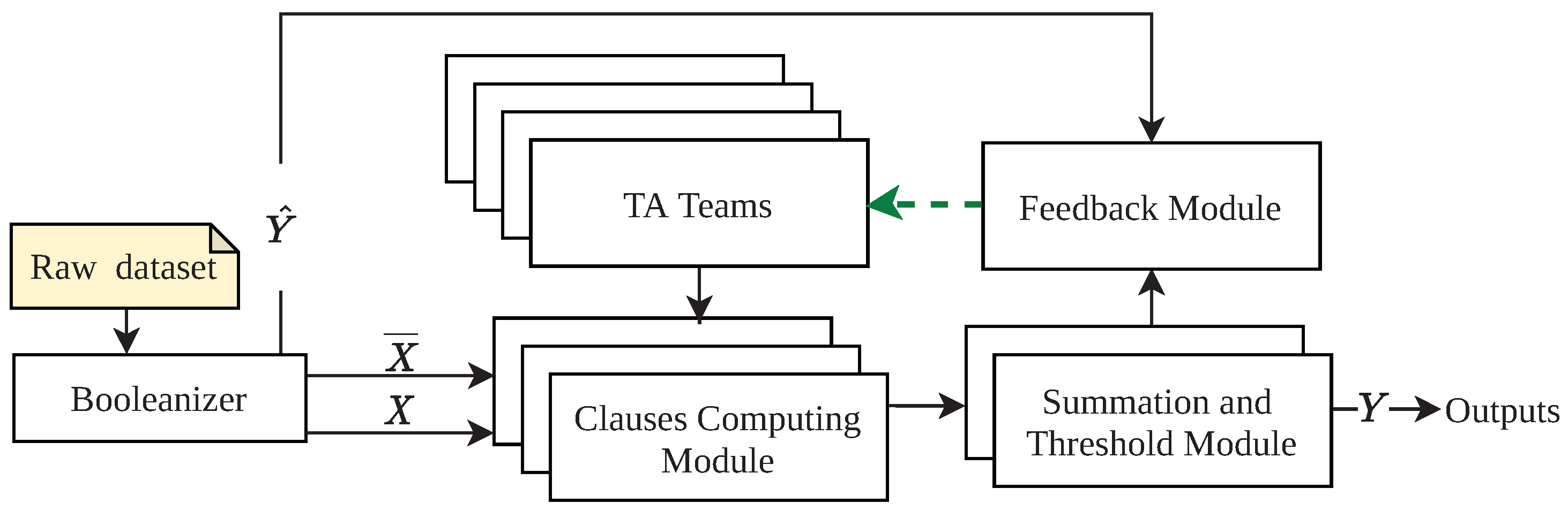
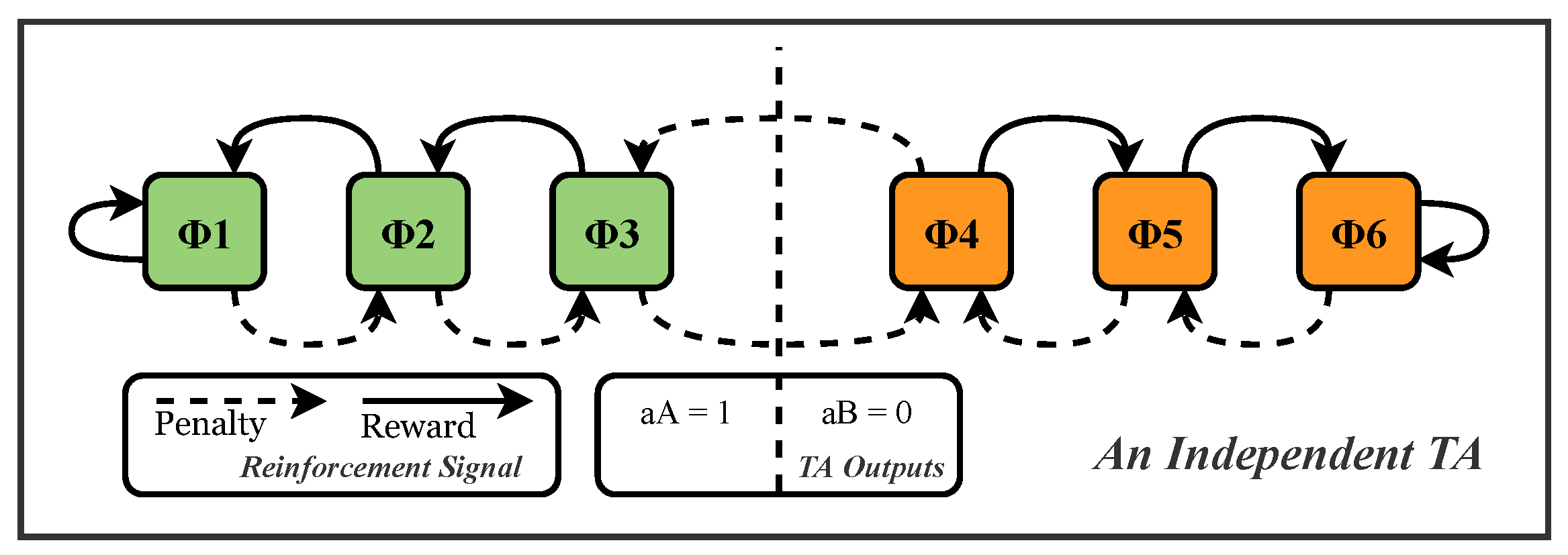
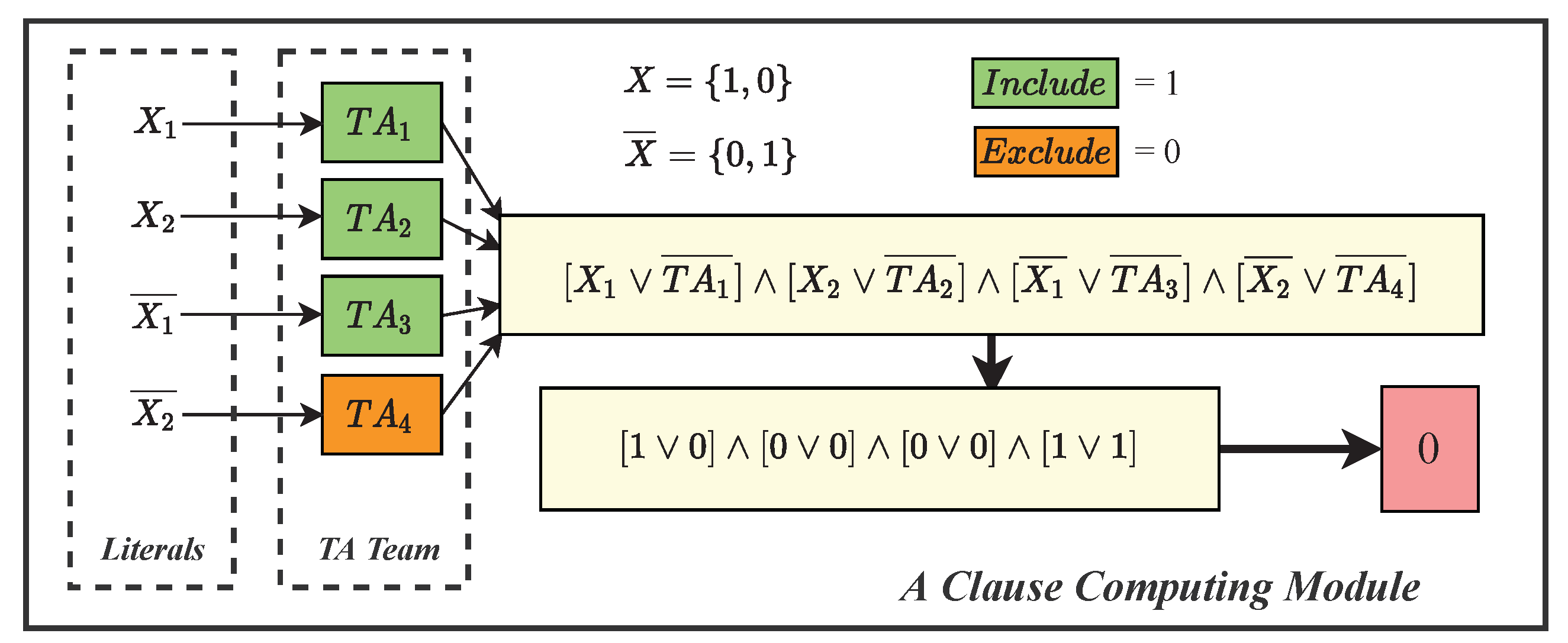
2. A Brief Introduction to Tsetlin Machine

The Tsetlin Machine is a promising, new ML algorithm based on formulation of propositional logic [16]. This section offers a high level overview of the main functional blocks; a detailed review of relevant research progress can be found in Section 5.2.

The core components of the Tsetlin Machine are: a team of Tsetlin Automata (TA) in each clause, conjunctive clauses, summation and threshold module and the feedback module, as seen in Figure 1. The TA are finite state machines (FSMs) that are used to form the propositional logic-based relationships that describe an output class through the inclusion or exclusion of input features and their complements. The states of the TAs for each feature and its compliment are then aligned to a stochastically independent clause computation module. Through a voting mechanism built into the summation and threshold module, the expected output class Y is generated. During the training phase, this class is compared against the target class $\hat{Y}$ and the TA states are incremented or decremented accordingly (this is also referred to as as issuing rewards or penalties).

A fundamental difference between the TM and NNs is the requirement of a Booleanizer module. The key premise is to convert the raw input features and their complements to Boolean features rather than binary encoded features as seen with NNs. These Boolean features are also referred to as literals: $\hat{X}$ and X. Current research has shown that significance-driven Booleanization of features for the Tsetlin Machine is vital in controlling the Tsetlin Machine size and processing requirements [18]. Increasing the number of features will increase the number of TA and increase computations for the clause module and subsequently the energy spent in incrementing and decrementing states in the feedback module. The choice of the number of clauses to represent the problem is also available as a design knob, which also directly affects energy/accuracy tradeoffs [19].

The Tsetlin Machine also has two hyperparameters, the s value and the Threshold (T). The Threshold parameter is used to determine the clause selection to be used in the voting mechanism, larger Thresholds will mean more clauses partake in the voting and influence the feedback to TA states. The s value is used to control the fluidity with which the TAs can transition between states. Careful manipulation of these parameters can be used to determine the flexibility of the feedback module and therefore control the TMs learning stability [17]. Figure 2 states the number of Penalty and Reward events that have been triggered by the feedback module of the TM when training on data from the Breast Cancer (Wisconsin) Diagnostic dataset. It indicates that increasing the Threshold and decreasing the s value will lead to more events triggered as more states are transitioned. These parameters must be carefully tuned to balance energy efficiency through minimizing events triggered, and achieving good performance through finding the optimum s–T range for learning stability in the KWS application.

In order to optimize the TM for KWS, due diligence must be given to designing steps that minimize the Boolean feature set. This allows for finding a balance between performance and energy usage through varying the TM hyper parameters and the number of clause computation modules. Through exploitation of these relationships and properties of the TM, the KWS pipeline can be designed with particular emphasis on feature extraction and minimization of the number of the TMs clause computation modules. An extensive algorithmic description of Tsetlin Machine can be found in [16]. The following section will detail how these ideas can be implemented through audio pre-processing and Booleanization techniques for KWS.

3. Audio Pre-Processing Techniques for KWS

When dealing with audio data, the fundamental design efforts in pre-processing should be to find the correct balance between reducing data volume and preserving data veracity. That is, while removing the redundancies from the audio stream, the data quality and completeness should be preserved. This is interpreted in the proposed KWS-TM pipeline through two methods: feature extraction through Mel-frequency cepstrum coefficients (MFCCs), followed by discretization control through quantile based binning for Booleanization. These methods are expanded below.

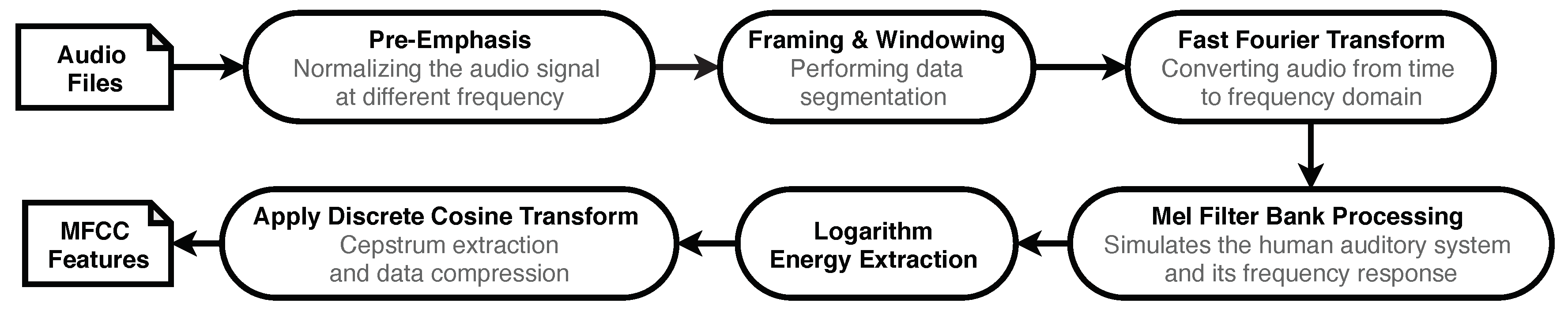
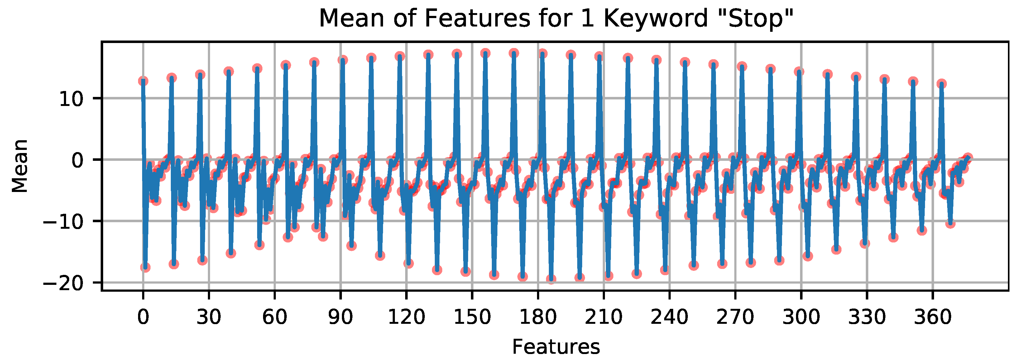
3.1. Audio Feature Extraction Using MFCC

Audio data streams are always subject to redundancies in the channel that formalize as nonvocal noise, background noise and silence [20,21]. Therefore, the challenge becomes identification and extraction of the desired linguistic content (the keyword) and maximally discarding everything else. To achieve this we must consider transformation and filtering techniques that can amplify the characteristics of the speech signals against the background information. This is often done through the generation of MFCCs as seen in the signal processing flow in Figure 3.

The MFCC is a widely used audio file pre-processing method for speech related classification applications [21,22,23]. The component blocks in the MFCC pipeline are specifically designed for extracting speech data taking into account the intricacies of the human voice.

The Pre-Emphasis step is used to compensate for the structure of the human vocal tract and provide initial noise filtration. When producing glottal sounds when speaking, higher frequencies are damped by the vocal tract which can be characterized as a step roll-off in the signals’ frequency spectrum [24]. The Pre-Emphasis step, as its name-sake suggests, amplifies (adds emphasis to) the energy in the high frequency regions, which leads to an overall normalization of the signal.

Speech signals hold a quasi-stationary quality when examined over a very short time period, which is to say that the statistical information it holds remains near constant [20]. This property is exploited through the Framing and Windowing step. The signal is divided into a sequence of time frames onto which an overlapping window function is applied. The need for overlapping windows is due to the tapering effect of the signal amplitude caused by the window function, the overlapping reduces these diminishing effects and thus preserves the temporal changes of the signal and minimize discontinuities (this is realized through the smoothed spectral edges and enhanced harmonics of the signal after the subsequent transformation to the frequency domain) [25]. The length of the window function (with respect to time) as well as the time offset between overlapping windows are design parameters that can be adjusted for different applications. The windowed signals are then transformed to the frequency domain through a Discrete Fourier Transform (DFT) process using the Fast Fourier Transform (FFT) algorithm. FFT is chosen as it is able to find the redundancies in the DFT and reduce the amount of computations required offering quicker run-times.

The human hearing system interprets frequencies linearly up to a certain range (around 1 KHz) and logarithmically thereafter. Therefore, adjustments are required to translate the FFT frequencies to this non-linear function [26]. This is done through passing signal through the Mel Filter Banks in order to transform it to the Mel Spectrum [27]. The filter is realized by overlapping band-pass filters to create the required warped axis. Next, the logarithm of the signal is taken, this brings the data values closer and less sensitive to the slight variations in the input signal [27]. Finally we perform a Discrete Cosine Transform (DCT) to take the resultant signal to the Cepstrum domain. The DCT function is used as energies present in the signal are very correlated as a result of the overlapping Mel Filter Banks and the smoothness of the human vocal tract; the DCT finds the co-variance of the energies and is used to calculate the MFCC features vector [28]. This vector can be passed to the Booleanizer module to produce the input Boolean features, as described next.

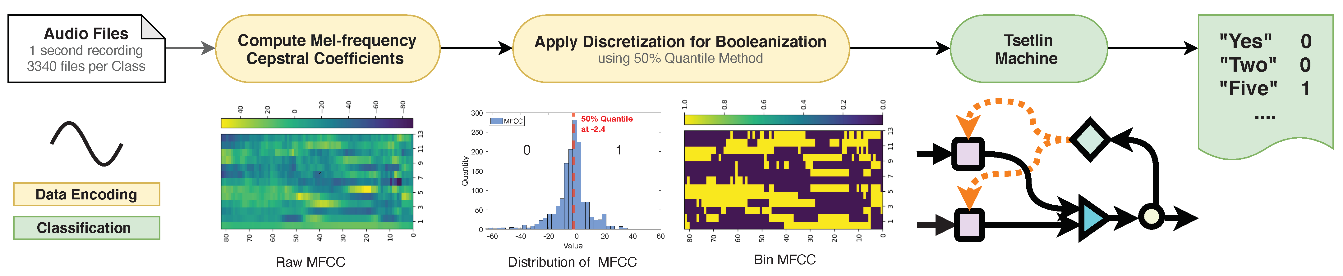
3.2. Feature Booleanization

As described in Section 2, Booleanization is an essential step for logic based feature extraction in Tsetlin Machines. Minimizing the Boolean feature space is crucial to the Tsetlin Machine’s optimization. The size and processing volume of a TM are primarily dictated by the number of Booleans [18]. Therefore, a pre-processing stage for the audio features must be embedded into the pipeline before the TM to allow for granularity control of the raw MFCC data. The number of the Booleanized features should be kept as low as possible while capturing the critical features for classification [18].

The discretization method should be able to adapt to, and preserve the statistical distribution of the MFCC data. The most frequently used method in categorizing data is through binning. This is the process of dividing data into groups, individual datapoints are then represented by the group they belong to. Data points that are close to each other are put into the same group thereby reducing data granularity [16]. Fixed width binning methods are not effective in representing skewed distribution and often result in empty bins, they also require manual decision making for bin boundaries.

Therefore, for adaptive and scalable Booleanization, quantile-based binning is preferred. Through binning the data using its own distribution, we maintain their statistical properties and do not need to provide bin boundaries, merely the number of bins the data should be discretized into. The control over the number of quantiles is an important parameter in obtaining the final Boolean feature set. Choosing two quantiles will result in each MFCC coefficient being represented using only one bit, either 0 or 1 based on its distribution, the Boolean representations for the datapoints are therefore the binarizations of the numerical value of the quantile to which the datapoint belongs. Therefore, the greater the number of quantiles, the greater the number of bits required to represent the quantile’s numerical value in binary, for example, choosing 10 quantiles (or bins) will result in 4 bits per coefficient. Given the large number of coefficients present in the KWS problem, controlling the number of quantiles is an effective way to reduce the total TM size.

Future work will aim to explore other Booleanization techniques in terms of performance, data reduction ability and robustness. These techniques include Histogram Equalization as well as mean and variance normalization methods as seen in [29,30,31]. The addition of noise in acoustic environments can lead to differing probability distributions between different samples recorded in different environments, using methods like Histogram Equalization can be effective in transitioning the MFCC features to a reference domain less effected by environmental effects [31].

3.3. The KWS-TM Pipeline

The KWS-TM pipeline is composed of the data encoding and classification blocks presented in Figure 4. The data encoding scheme encompasses the generation of MFCCs and the quantile binning-based Booleanization method. The resulting Booleans are then fed to the Tsetlin Machine for classification. The figure highlights the core attributes of the pre-processing blocks: the ability to extract the audio features only associated with speech through MFCCs and the ability to control their Boolean granularity through quantile binning.

To explore the functionality of the pipeline and the optimizations that can be made, we return to our primary intentions, i.e., to achieve energy efficiency and high learning efficacy in KWS applications. We can now use the design knobs offered in the pre-processing blocks, such as variable window size in the MFCC generation, and control over the number of quantiles to understand how these parameters can be used in presenting the Boolean data to the TM in a way to returns good performance utilizing the least number of Booleans. Through Section 2, we have also seen the design knobs available through variation of the hyperparameters s and Threshold T, as well as the number of clause computation modules used to represent the problem. Varying the parameters in both the encoding and classification stages through an experimental context will uncover the impact they have on the overall KWS performance and energy usage. The MFCCs used were all static and the exploration of first and second order frame-to-frame differences through dynamic delta and delta-delta MFCCs will be explored in future work.

4. Experimental Results

To evaluate the proposed KWS-TM pipeline, Tensorflow speech command dataset was used (Tensorflow speech command: https://tinyurl.com/TFSCDS, Accessed: 8 April 2021). The dataset consists of many spoken keywords collected from a variety of speakers with different accents, as well as male and female gender. The datapoints are stored as 1 s long audio files where the background noise is negligible. This reduces the effect of added redundancies in the MFCC generation, given our main aim is predominantly to test functionality, we will explore the impact of noisy channels in our future work. This dataset is commonly used in testing the functionality of ML models and will therefore allow for fair comparisons to be drawn [32].

From the Tensorflow dataset, 10 keywords: “Yes”, “No”, “Stop”, “Seven”, “Zero”, “Nine”, “Five”, “One”, “Go” and “Two”, have been chosen to explore the functionality of the pipeline using some basic command words. Considering other works comparing NN-based pipelines, 10 keywords is the maximum used [13,33]. Among the keywords chosen, there is an acoustic similarity between “No” and “Go”, therefore, we explore the impact of 9 keywords together (without “Go”) and then the effect of “No” and “Go” together. The approximate ratio of training data, testing data and validation data is given as 8:1:1 respectively with a total of 3340 datapoints per class. Using this setup, we will conduct a series of experiments to examine the impact of the various parameters of the KWS-TM pipeline discussed earlier. The experiments are as follows:

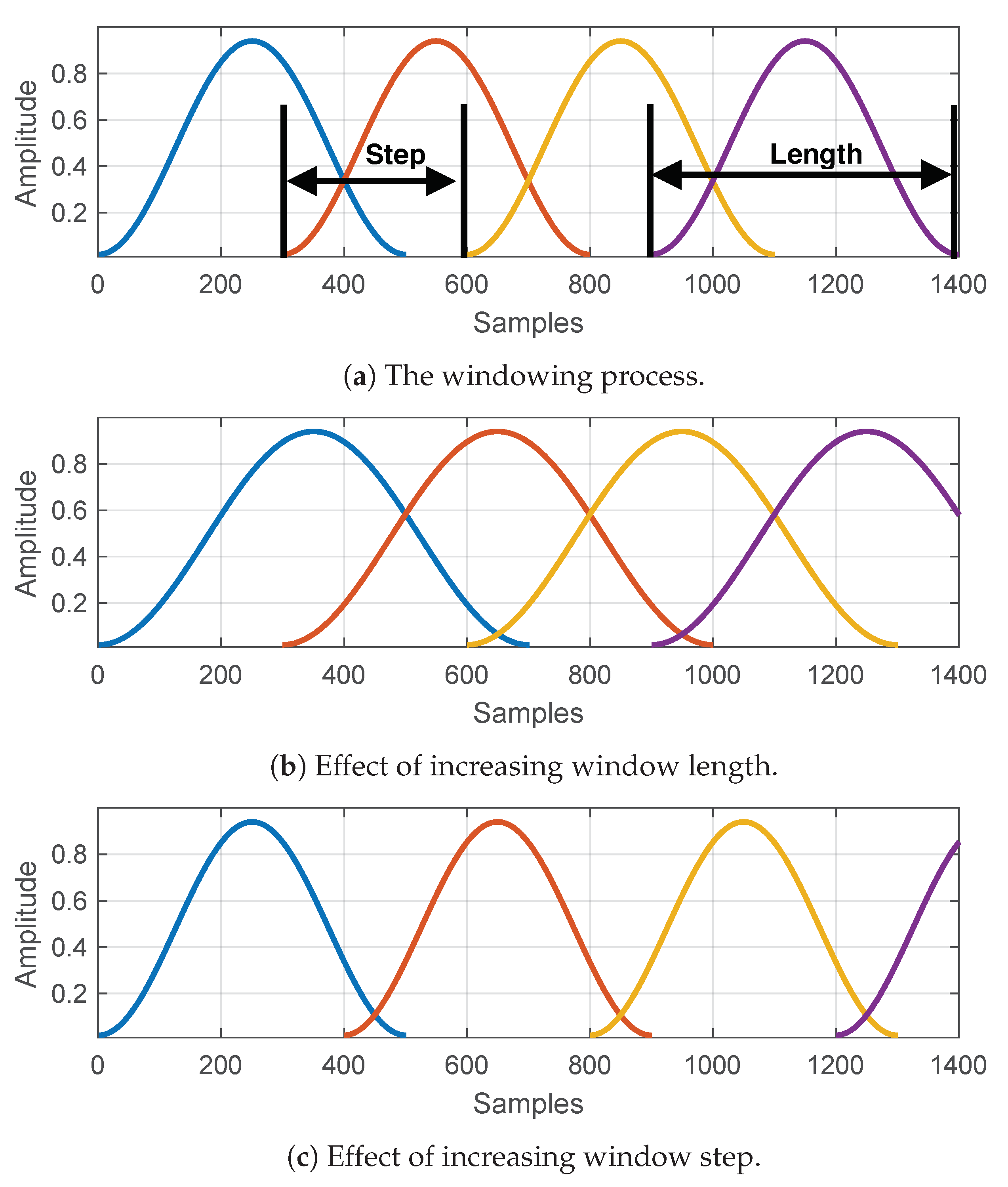
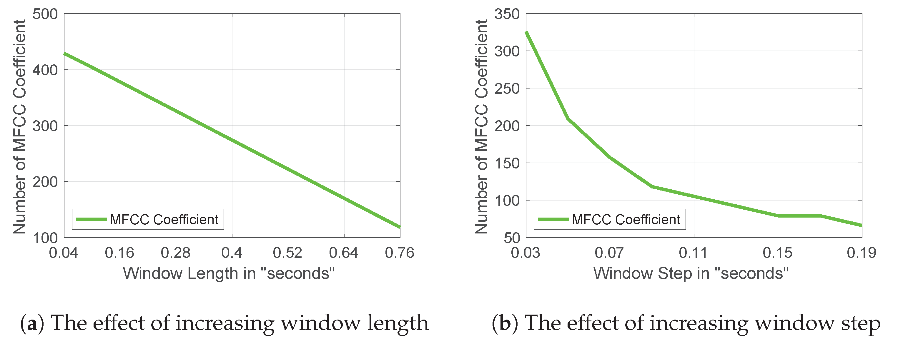
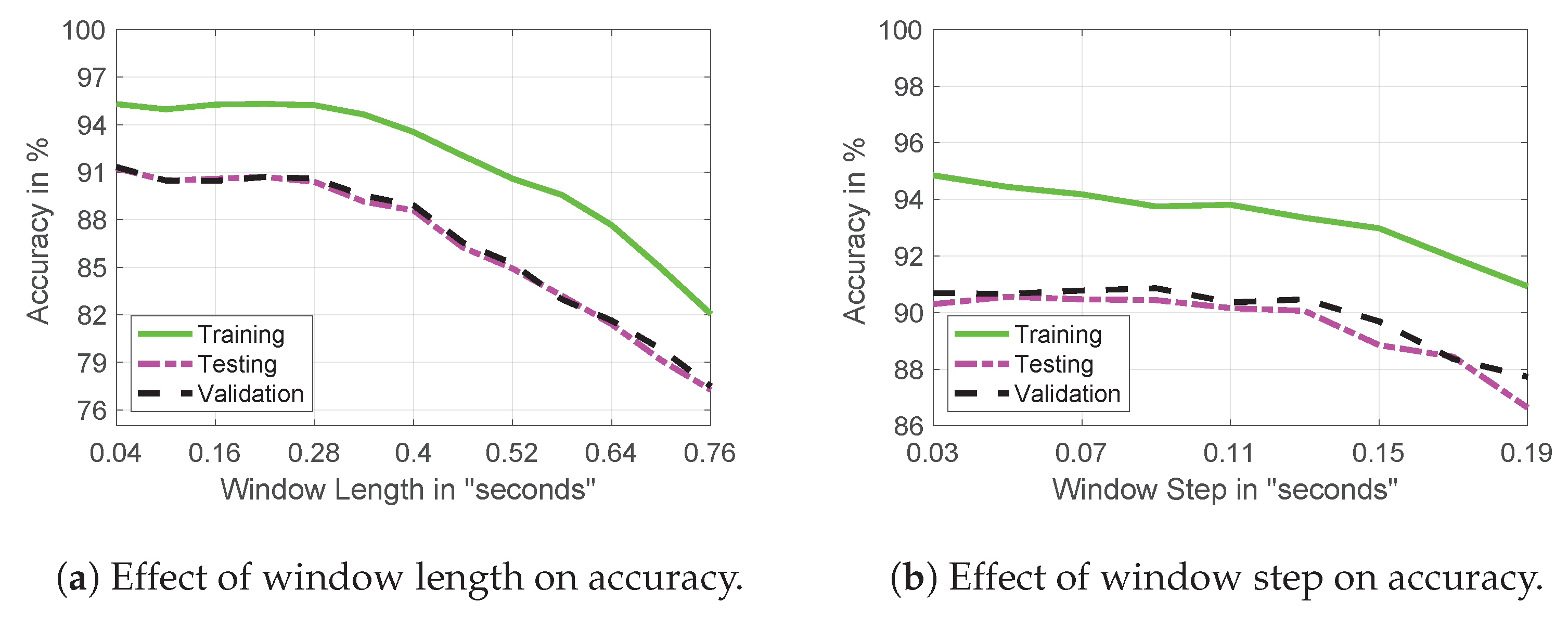
• Manipulating the window length and window steps to control the number of MFCCs generated.
• Exploring the effect of different quantile bins to change the number of Boolean features.
• Using a different number of the keywords ranging from 2 to 9 to explore the scalability of the pipeline.
• Testing the effect on performance of acoustically different and similar keywords.
• Changing the size of the TM through manipulating the number of clause computation modules, optimizing performance through tuning the feedback control parameters s and T.

4.1. MFCC Setup

It is well defined that the number of input features to the TM is one of the major factors that affect its resource usage [17,18,19]. Increased raw input features means more Booleans are required to represent them and thus the number of Tsetlin Automaton (TA) in the TM will also increase leading to more energy required to provide feedback to them. Therefore, reducing the number of features at the earliest stage of the data encoding stage of the pipeline is crucial to implementing energy-frugal TM applications.

The first set of parameters available in manipulating the number of features comes in the form of the window step and the window length (this takes place in the “Framing a Windowing” stage in Figure 4) in MFCC generation and can be seen through Figure 5a.

The window function is effective in reducing the spectral distortion by tapering the sample signal at the beginning and ending of each frame (We use overlapping frames to ensure signal continuity is not lost). Smaller Window Steps lead to a more fine grained and descriptive representation of the audio features through more frames and therefore more MFCCs but this also increases computations and latency. Thus, we explored the impact of different windowing parameters with same setup: 4 keywords, 13 MFCC coefficients per frame, 13 MFCC coefficients per frame, 1 Boolean to represent eachMFCC feature, 240 clauses per class, s value of 6 and threshold T set to 17.

Increasing the window length (with 0.03 s window step) leads to a linear decrease in the total number of frames and therefore the MFCCs as seen in Figure 6a. Given that the Window Steps are kept constant for this experiment, we have a linearly decreasing number of window overlaps resulting in a linearly decreasing total number of window functions, FFTs and subsequent computations. This leads to the linear decrease in the MFCCs across all frames.

Increasing the window step (with 0.28 s window length) leads to much sharper fall given the overlapping regions now no longer decrease linearly as seen in Figure 6b. This results in a total number of non-linearly decreasing window functions and therefore much fewer FFTs and so on, leading to much fewer MFCCs across all frames. As a result of this, the smaller the increase in the window step the larger the decrease in the number of frames and therefore MFCCs.

To test the effectiveness of manipulating the window length and window step (seen visually through Figure 5), the MFCC coefficients were produced for 4 keywords and the TM classification performance was examined as seen in Figure 7a,b. Changing the window length results in much bigger falls in accuracy compared to window step. Increasing the window above around 0.3 s, as seen in Figure 7a, shows that the signal is most likely become non-stationary when considered through longer windows and this is related to the fall in accuracy. The effect of increasing the window step reduces the overlap of the windows (see Figure 5c) and therefore the cross-correlation of the signal frames, as such fewer of the signals dynamics are captured and this results in the reduced accuracy with increasing step size. The impact of this is relatively small (around a 2% in accuracy) given that the window length is sufficiently large enough to provide high frequency resolution but also small enough such that the signal still shows stationary characteristics.

We can see that increasing the window step is very effective in reducing the number of frames and therefore the total number MFCC coefficients across all frames and providing the window length is long enough, the reduction in performance is minimal. To translate these findings toward energy efficient implementations, we must give increased design focus to finding the right balance between the size of the window step parameter and the achieved accuracy given the reduction in computations from the reduction in features produced.

4.2. Impact of Number of Quantiles

Increased granularity through more bins will lead to improved performance but it is observed that this is not the case entirely.

Table 1. Impact of increasing quantiles with 4 classes.

Training	Testing	Validation	Num. Bins	Bools per Feature	Total Bools
94.8%	91.3%	91.0%	2	1	377
96.0%	92.0%	90.7%	4	2	757
95.9%	90.5%	91.0%	6	3	1131
95.6%	91.8%	92.0%	8	3	1131
97.1%	91.0%	90.8%	10	4	1511

shows the impact of the KWS-TM (4 keywords, window length of 0.16 s, window step of 0.03 s, 13 MFCC coefficients per frame, 240 clauses per class, s set to 6, T set to 17) performance when increasing the number of bins. The testing and validation accuracy remain around the same with 1 Boolean per feature compared with 4 Booleans per feature. We also analyse the mean and variance values of 377 features in a 1 s audio of “Stop” over 640 different datapoints. The 377 features were created by appending the 13 MFCC features from all 29 frames. Figure 8 and Figure 9 were created by calculating the mean and variance of each individual feature across all 640 datapoints for the keyword. Figure 8 shows the large variance in some feature columns and no variance in others. The zero variance features are redundant in the subsequent Booleanization, they will be represented through the same Boolean sequence. The features with large variances are of main interest. We see that the mean for these features is relatively close to zero compared to their variance (as seen in Figure 9), therefore one Boolean per feature representation is sufficient, a 1 will represent values above the mean and 0 will represent below. The logical conclusion to be made from these explorations is that the MFCC alone is sufficient in both eliminating redundancies and extracting the keyword properties and does not require additional granularity beyond one Boolean per feature to distinguish classes.

We have seen that the large variance of the MFCCs means that they are easily represented by 1 Boolean per feature and that is sufficient to achieve high performance; however, this is most likely task specific as we limit our experiments to 10 keywords with no background noise. Future work will aim to examine and optimize the Booleanization strategy for performance, scalability and combating noise. Nevertheless, this is an important initial result, for offline learning we can now also evaluate the effect of removing the no variance features in future work to further reduce the total number of Booleans. From the perspective of the Tsetlin Machine, there is an additional explanation as to why the performance remains high even when additional Boolean granularity is allocated to the MFCC features. Given that there are a large number datapoints in each class (3340), if the MFCCs that describe these datapoints are very similar then the TM will have more than sufficient training data to settle on the best propositional logic descriptors. This is further seen by the high training accuracy compared to the testing and validation accuracy.

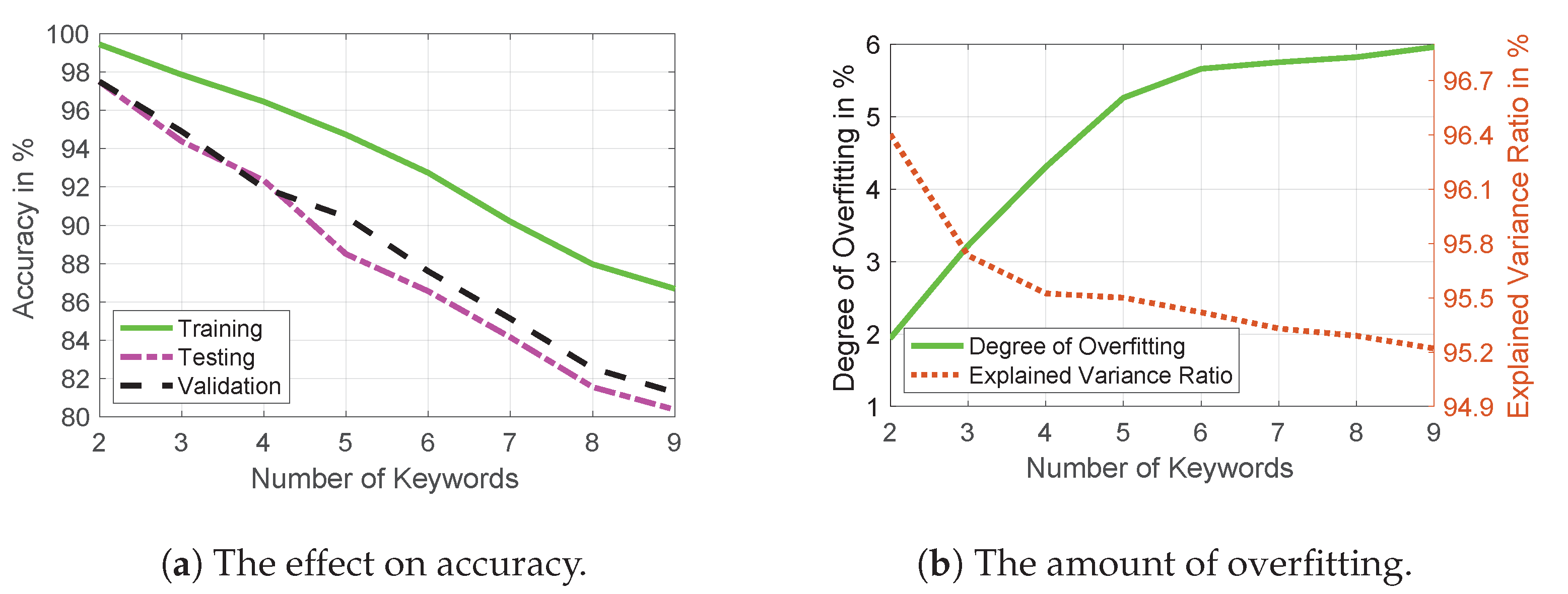
4.3. Impact of Increasing the Number of Keywords

In this section, we explored the accuracy changes at different number of keywords with the same setup: window length 0.16 s, window step 0.03 s, 13 MFCC coefficients per frame, 377 MFCC features with 1 Boolean representation, 240 clauses per class, s set to 6 and T set to 17.

Figure 10a shows the linear nature with which the training, testing and validation accuracy decrease as the number of keywords are increased for a TM with 450 clauses with 200 epochs for training. We note that the testing and validation accuracy start to veer further away from the training accuracy with the increase of keywords. This performance drop is expected in ML methods as the problem scales [34]. We evaluated the degree of overfitting of the TM through calculating the difference in accuracy between the training data and mean of validation and testing data accuracies as shown in Equation (1).

$$DegreeofOverfitting=Acc{u}_{Train}-\frac{Acc{u}_{Vali}+Acc{u}_{Test}}{2}$$

(1)

Despite the large number of datapoints per keyword, this is an indicator of overfitting, as confirmed through Figure 10b showing around a 4% increase. The implication of this is that increased number of keywords make it difficult for the TM to create distinct enough propositional logic to separate the classes. The performance drop is caused when the correlation of keywords outweighs the number of datapoints to distinguish each of them. This behaviour is commonly observed in ML models for audio classification applications [35].

The explained variance ratio of the dataset, when increasing the number of keywords, was derived by taking the first 100 Principle Component Analysis eigenvalues, calculated based on the MFCC features, as seen in Figure 10b. We observe that as the number of keywords is increased, the system variance decreases, i.e., the inter-class features start to become increasingly correlated. Correlated inter-class features will lead to class overlap and degrade TM performance [18]. Through examination of the two largest Linear Discriminant component values for the 9 keyword dataset, we clearly see in Figure 11 that there is very little class separability present.

To mitigate against the effect on performance of increasing keywords, there are two methods available: Firstly, to adjust the Tsetlin Machine hyperparameters to enable more events triggered (see Figure 2). In doing so the this may allow the TM to create more differing logic to describe the classes. Then, by increasing the number of clause computation modules, the TM will have a larger voting group in the Summation and Threshold module and potential reach the correct classification more often. Secondly the quantity of the datapoints can be increased, however, for this to be effective the new dataset should hold more variance and completeness when describing each class. This method of data regularization is often used in audio ML applications to deliberately introduce small variance between datapoints [21].

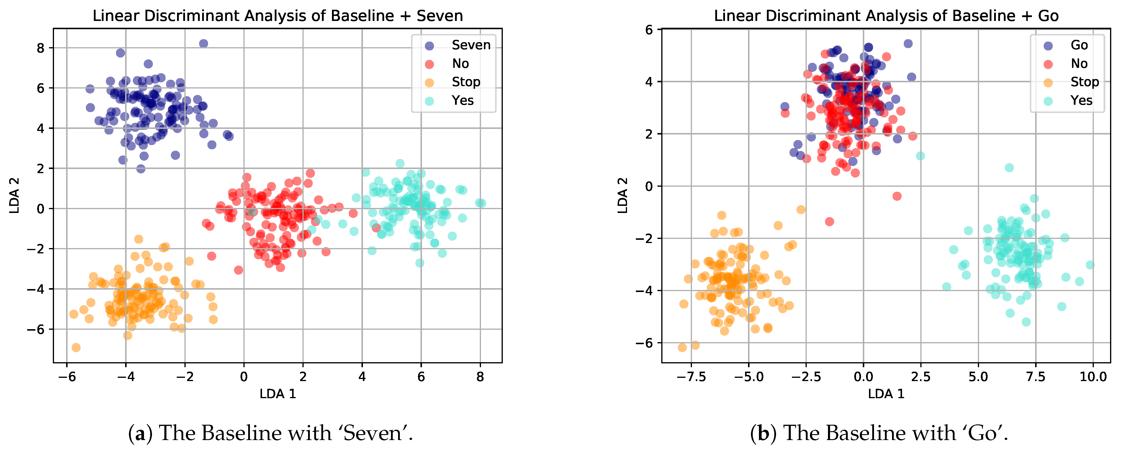
4.4. Acoustically Similar Keywords

In order to test the robustness of the KWS-TM pipeline functionality, we must emulate real-word conditions where a user will use commands that are acoustically similar to others.

Table 2. Impact of acoustically similar keywords.

Experiments	Training	Testing	Validation
Baseline	94.7%	92.6%	93.1%
Baseline + ‘Seven’	92.5%	90.1%	90.2%
Baseline + ‘Go’	85.6%	82.6%	80.9%

shows the results of such circumstances. The Baseline experiment is a KWS dataset consisting of 3 keywords: ‘Yes’, ‘No’ and ‘Stop’. The second experiment then introduces the keyword ‘Seven’ to the dataset and the third experiment introduces the keyword ‘Go’ (window length 0.16 s, window step 0.03 s, 13 MFCC coefficients per frame, 377 MFCC features with 1 bool representation, 240 clauses/class, s set to 6, T set to 17).

The addition of ‘Seven’ causes a slight drop in accuracy adhering to our previously made arguments of increased correlation and the presence of overfitting. However, the key result is the inclusion of ‘Go’; ‘Go’ is acoustically similar to ‘No’ and this increases the difficulty in separating these two classes. We see from Figure 12a, showing the first two LDA components that adding ‘Seven’ does not lead to as much class overlap as adding ‘Go’ as seen in Figure 12b. As expected, the acoustic similarities of ‘No’ and ‘Go’ lead to significant overlap. We have seen from the previous result (Figure 11) that distinguishing class separability is increasingly difficult when class overlaps are present.

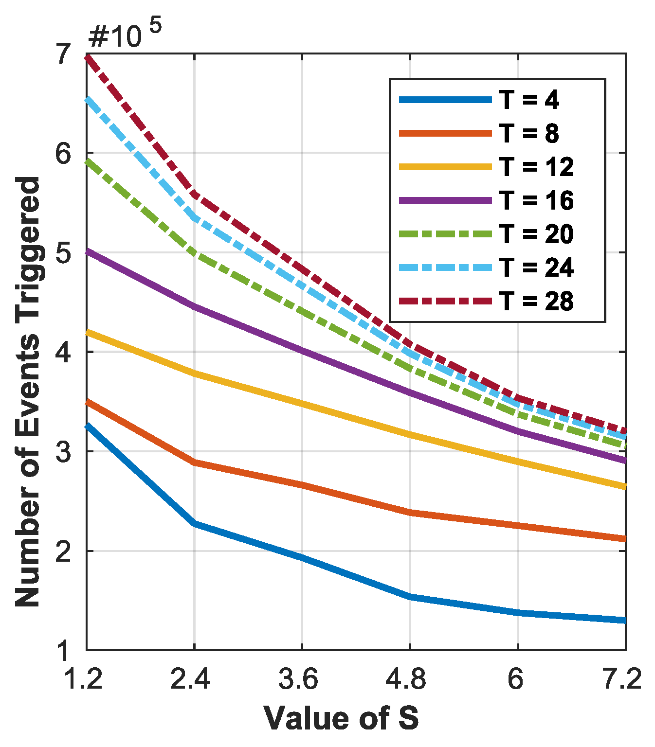
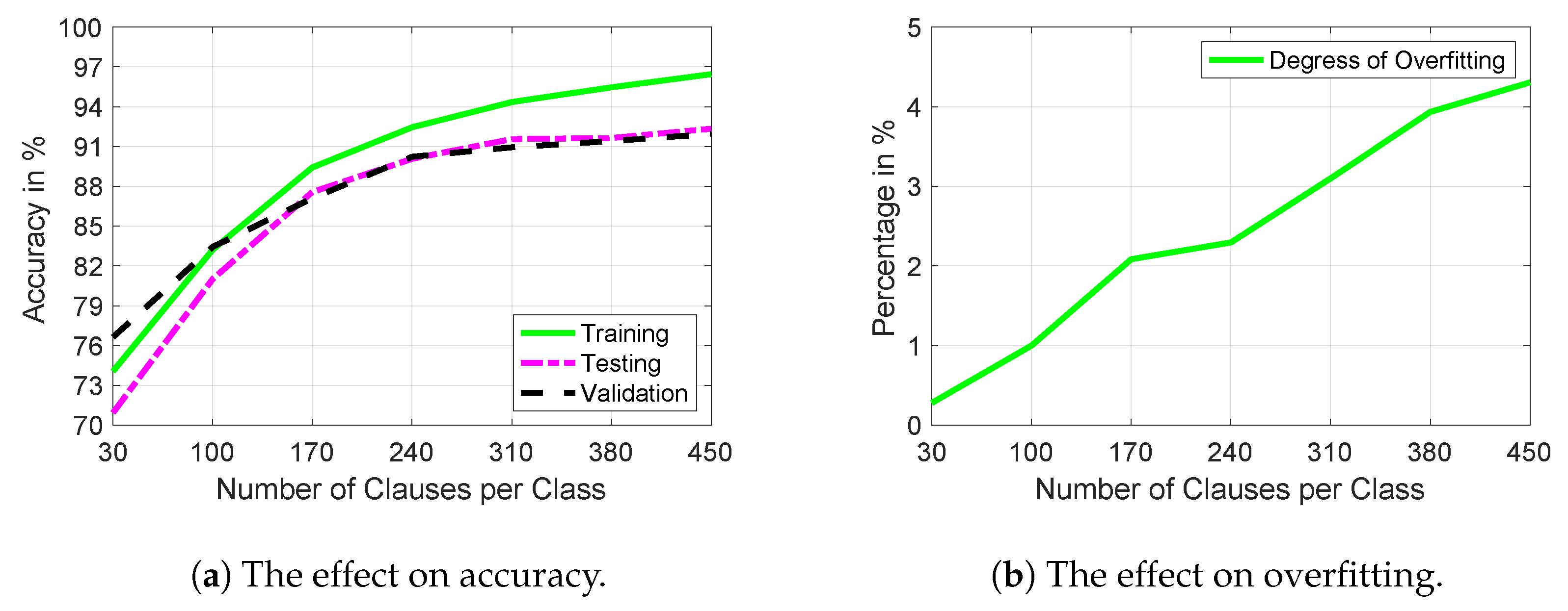
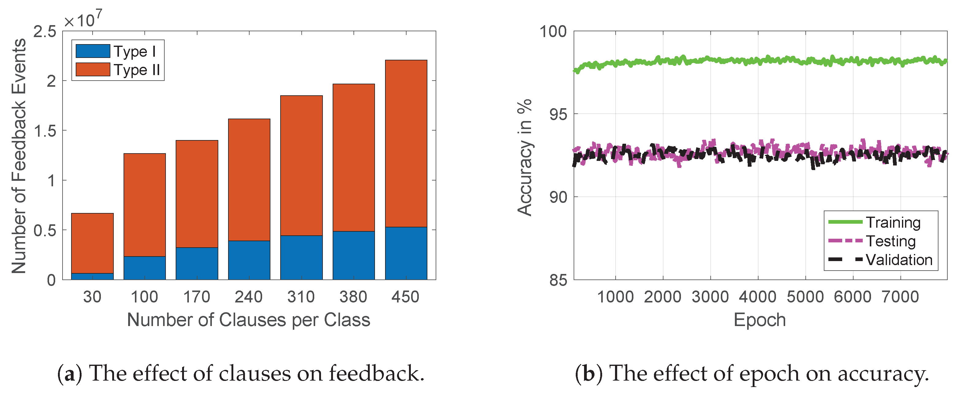
4.5. Number of Clauses per Class

So far we have considered the impact of Booleanization granularity, problem scalabilty and robustness when dealing with acoustically similar classes. Now, we turn our attention towards optimizing the KWS-TM pipeline to find the right functional balance between performance and energy efficiency. This is made possible through two streams of experimentation: manipulating the number of clauses for each keyword class in the TM and observing the energy expenditure and accuracy, and experimenting with the TM hyperparameters to enable better performance using fewer clauses.

The influence of increasing the number of clauses was briefly discussed in Section 2, here we can see the experimental result in Figure 13a showing the impact of increasing clauses with 4 classes, window length 0.16 s, window step 0.03 s, 377 MFCC with 1 bool representation, s set to 6 and T set to 17.

Increased number of clauses leads to better performance. However, upon closer examination we can also see the impact of overfitting at the clause level, i.e., increasing the number of clauses has resulted in a larger difference in the training accuracy with the testing and validation. The datapoints for the 4 classes were sufficient to create largely different sub-patterns for the TAs during training, but not complete enough to describe new data in the testing and validation. As the number of classes increases we must also increase the number of training data instances to match the problem scale in order to improve the degree of overfitting (see Equation (1)). In addition to fewer training datapoints there is also the issue of class overlapping leading to less separability and poorer performance.

As a result, when clauses are increased, more clauses reach incorrect decisions and sway the voting in the summation and threshold module toward incorrect classification, which is seen through Figure 14a. The TM has two types of feedback, Type I, which introduces stochasticity to the system and Type II, which bases state transitions on the results of corresponding clause value. Type II feedback is predominantly used to diminish the effect of false positives. We see that as the clause value increases the TM uses more Type II feedback indicating increased false positive classifications. This result is due to the incompleteness in the training data in describing all possible logic propositions for each class. Despite increasing the number of epochs, we do not experience a boost in testing and validation accuracy and through Figure 13b we find the point where the overfitting outweighs the accuracy improvement at around 190–200 clauses.

From the perspective of energy efficiency, these results offer two possible implications for the KWS-TM pipeline, if a small degradation of performance in the KWS application is acceptable, then operating at a lower clause range will be more beneficial for the TM. The performance can then be boosted through hyperparameters available to adjust feedback fluidity. This approach will reduce energy expenditure through fewer clause computations and reduce the effects of overfitting when the training data lacks enough completeness. Alternatively, if performance is the main goal, then the design focus should be on injecting training data with more diverse datapoints to increase the descriptiveness of each class. In that case, increased clauses will provide more robust functionality.

The impacts of being resource efficient and energy frugal are most prevalent when implementing KWS applications into dedicated hardware and embedded systems. To explore this practically, the KWS-TM pipeline was implemented onto a Raspberry Pi. The same 4 keyword experiment was ran with 100 and 240 clauses per class, window length of 0.16 s, window step of 0.03 s, 377 MFCC with 1 Boolean representation, S set to 6 and T set to 17. We calculated the energy consumed by the Python TM application through an external power analyser. As expected, we see that increased clause computations lead to increased current, time and energy usage, but also delivers better performance as seen in

Table 3. Impact of the number of clauses on energy/accuracy tradeoffs.

	Clauses	Current	Time	Energy	Accuracy
Training	100	0.50 A	68 s	426.40 J	-
Training	240	0.53 A	96 s	636.97 J	-
Inference	100	0.43 A	12 s	25.57 J	80%
Inference	240	0.47 A	37 s	87.23 J	90%

. We can potentially boost the performance of the Tsetlin Machine at lower clauses through manipulating the hyperparameters as seen

Table 4. Impact of the T values on accuracy.

Clauses	T	Training	Testing	Validation	Better Classification
30	2	83.5%	80.5%	83.8%	✓
30	23	74.9%	71.1%	76.1%
450	2	89.7%	86.1%	84.9%
450	23	96.8%	92.5%	92.7%	✓

.

The major factor that has impacted the performance of the KWS is the capacity of the TM which is determined by the number of clauses per class. The higher the number clauses, the higher the overall classification accuracy [18]. Yet, the resource usage will increase linearly along with the energy consumption and memory footprint. Through Table 4 we see that at 30 clauses the accuracy can be boosted through reducing the Threshold hyperparameter. The table offers two design scenarios; firstly, very high accuracy is achievable through a large number of clauses (450 in this case) and a large Threshold value. With a large number of clauses an increased number of events must be triggered in terms of state transitions (see Figure 2) to encourage more feedback to clauses and increases the TMs decisiveness. While this offers a very good return on performance, the amount of computations are increased with more clauses and more events triggered and this leads to increased energy expenditure as seen through Table 3.

In contrast, using a total of 450 clauses and a lower Threshold still yields good accuracy but at a much lower energy expenditure through fewer clause computations and feedback events. A smaller number of clauses mean that the vote of each clause has more impact, even at a smaller Threshold the inbuilt stochasticity of the TM’s feedback module allows the TAs to reach the correct propositional logic. Through these attributes, it is possible to create more energy frugal TMs requiring fewer computations and operating at a much lower latency.

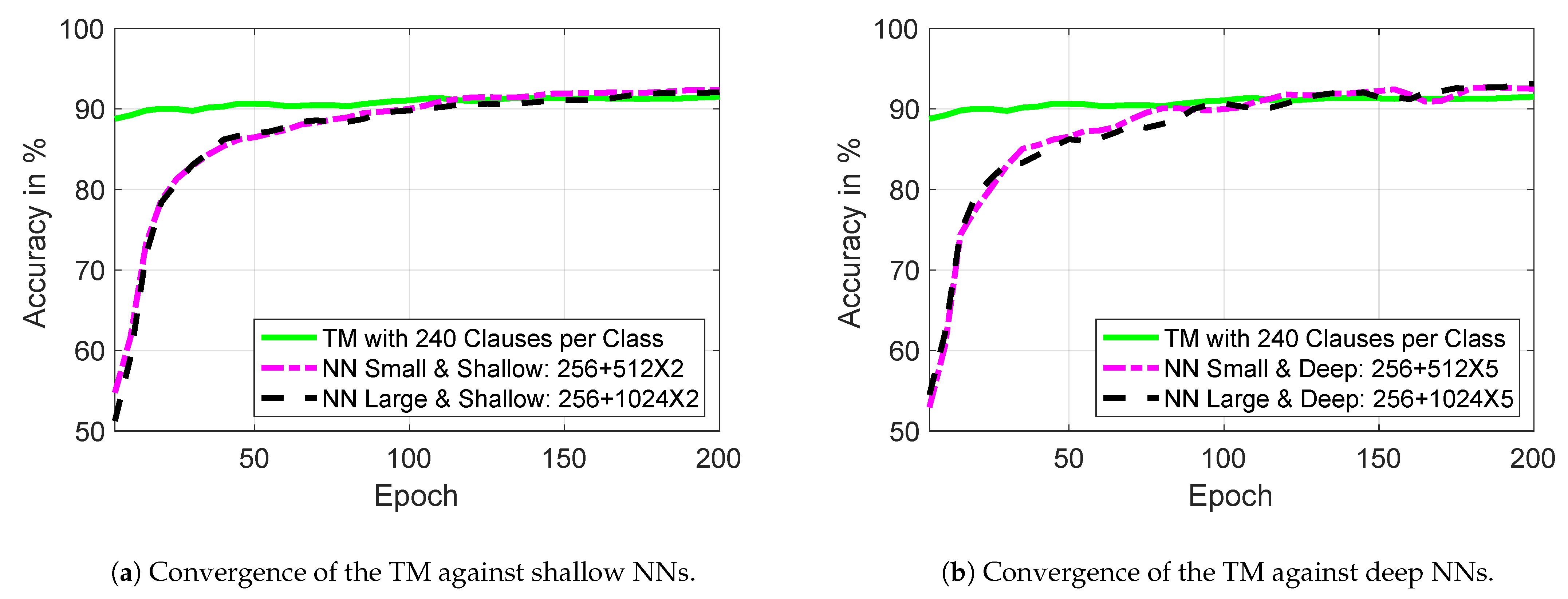
4.6. Comparative Learning Convergence and Complexity Analysis of KWS-TM

Both TMs and NNs have modular design components in their architecture; For the TM, this is in the form of clauses and for the NN it is the number of neurons. NNs require input weights for the learning mechanism which define the neurons’ output patterns. The number of weights and the number of neurons are variable, however more neurons will lead to better overall NN connectivity due to more refined arithmetic pathways to define a learning problem.

For the TM, the clauses are composed of TAs. The number of TAs are defined by the number of Boolean features which remains static throughout the course of the TMs learning. It is the number of clauses that is variable, increasing the clauses typically offers more propositional diversity to define a learning problem.

Through Figure 15 and

Table 5. The required parameters for different NNs and the TM for a 4 keyword problem.

KWS-ML Configuration	Num. Neurons	Num. Hyperparameters
NN Small & Shallow: 377 + 256 + 512 × 2 + 4	1661	983,552
NN Small & Deep: 377 + 256 + 512 × 5 + 4	3197	2,029,064
NN Large & Shallow: 377 + 256 + 1024 × 2 + 4	2.685	2,822,656
NN Large & Deep: 377 + 256 + 1024 × 5 + 4	5757	7,010,824
TM with 240 Clauses per Class	960 (clauses in total)	2 hyperparameters with 725,760 TAs

, we investigate the learning convergence rates of the TM against 4 ‘vanilla’ NN implementations. We use the same 4 keywords KWS dataset with window length 0.16 s, window step 0.03 s, 13 MFCC coefficients per frame, 377 MFCC features with 1 bool representation for the experiments. The two NN models are based on Tensorflow multilayer perceptron network with 0.05 learning rate and gradient descent. The NN models have 4 variations as seen in Table 5, the nomenclature of the different models can be seen as follows: ‘NN Large and Shallow’ consists 5 layers: the input layer (377 nodes), the first hidden layer (256 nodes), the second hidden layer (1024 nodes), the third hidden layer (1024 nodes) and the output layer (4 nodes). The parameters for the TM are clause/class set to 240, s set to 6 and T set to 17.

The TM is able to converge to 90.5% after less than 10 epochs highlighting its quick learning rate compared to NNs which require around 100 epochs to converge to the isoaccuracy target (≈90%). After further 100 epochs, the NN implementations reach only marginally better accuracy than TM. The indirect implication of faster convergence is improved energy efficiency as fewer training epochs will result in fewer computations required for the TA states to settle.

Table 5 shows one of the key advantages of the TM over all types of NNs, the significantly fewer parameters required, i.e., low-complexity. Large number of parameters needed for NNs are known to limit their practicality for on-chip KWS solutions [12,13,33,36], where as the TM offers a more resource-frugal alternative. With only 960 clauses in total, which require only logic-based processing, the TM outperforms even the most capable large and deep NNs. In our future work, we aim to exploit this to enable on-chip learning based KWS solutions.

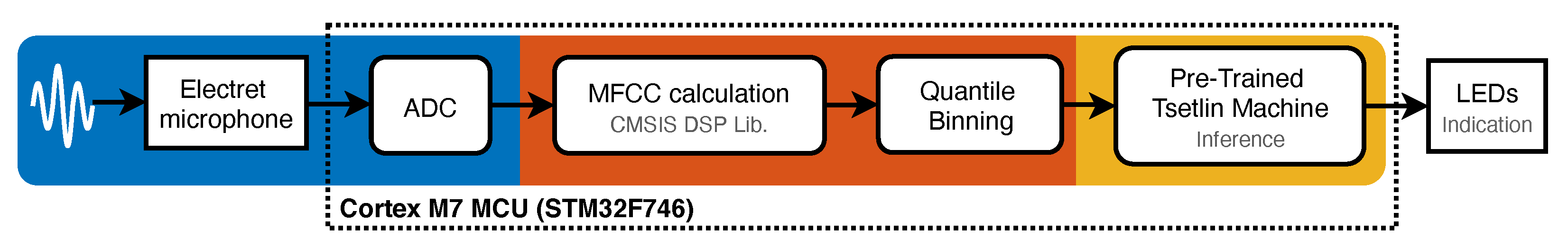
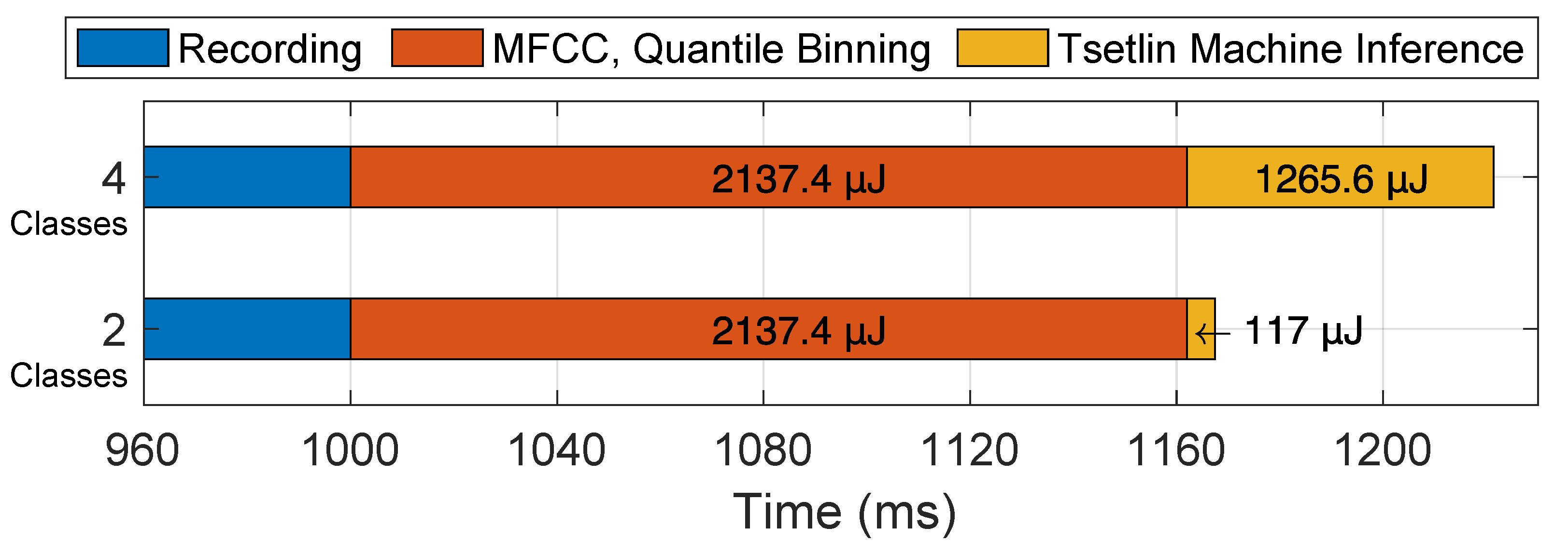
4.7. KWS-TM on the Embedded System

In order to demonstrate the energy-frugality of the TM, we deployed our MFCC-TM inference pipeline into an embedded system, the STM32F746 ARM Cortex M7 microcontroller. The demonstration video can be found in https://tinyurl.com/KWSTMDEMO, Accessed: 8 April 2021.

We chose two KWS scenarios to explore the functionality and energy-frugality of the MFCC-TM inference process on our embedded implementation: (1) using 2 classes (‘Yes’, ‘No’) with 10 clauses per class, (2) using 4 classes (‘Yes’, ‘No’, ‘Stop’, ‘Seven’) with 50 clauses per class. Both scenarios used 377 MFCC features, using a 0.16 s window length and 0.03 s window step, where each coefficient was represented by 1 Boolean digit.

In order to facilitate inference, the TM model was trained according to the two scenarios above and the TA states were saved into an array on the microcontroller flash memory. The microcontroller could then use these pre-configured states during the inference process. In the TM, it is only the settled TA states that hold the learned information and simply using these is enough to start inference.

As a proof of concept of MFCC-TM on the edge, we set an ISO-accuracy target of 88% to indicate a satisfactory performance. While we have shown accuracy can be improved through increasing the number of clauses, on our embedded device this will proportionally increase the memory footprint of the TM, which is restricted to an on-chip static RAM (SRAM) of 320KB for this specific microcontroller.

Figure 16 shows the system diagram of our MFCC-TM pipeline on the ARM Cortex M7 microcontroller. The design is similar with the Python pipeline (Figure 4) but it is configured for inference only and uses a microphone followed by an analog-to-digital (ADC) converter for audio pre-processing.

Initially, the microcontroller will load the pre-trained model and initialize the TM for inference. Then the inference can start by using the Analog-to-digital converter (ADC) to poll 1 s audio at 16 KHz sampling rate which has the same rate and duration as the training data. The ADC data will be segmented as 29 frames to calculate MFCC features (13 coefficient per frame as used in the training data) using Arm digital signal processing (DSP) library. Then the features will be Booleanized based on the dynamic quantile value.

In order to understand the behaviour of the TM on the microcontroller (at 216 MHz), we implemented the pipeline shown in Figure 4 and used an external power analyser to measure energy consumption excluding idle energy components.

The audio pre-processing time remained the same across the two experiments as seen in Figure 17 with 160 ms, of which approximately 0.7 ms was spent on quantile binning for both scenarios. The energy consumption for generating the input literals also remains the same (using 2137.4 µJ). As expected, the core difference in energy comes from the longer inference time for 4 classes.

For the 2-keyword KWS, it only requires 10 clauses per class for the TM to reach the target. However the 4-keyword problem requires 5X as many clauses per class due to the increasing feature overlaps. Increasing the scale of KWS problem will directly impact the number of TAs in the system. For 2 keywords with 10 clauses per class setup, the total number of TAs are 15.8 K, as calculated by the Equation (2):

$$\begin{array}{c}\hfill Nu{m}_{TAs}=Nu{m}_{Literals}\times 2\times Nu{m}_{Class}\times Nu{m}_{Clauses};\\ \hfill Nu{m}_{2ClassesTAs}=377\times 2\times 2\times 10=15,080;\\ \hfill Nu{m}_{4ClassesTAs}=377\times 2\times 4\times 50=150,800.\end{array}$$

(2)

The larger 4-keyword problem requires 10 times more TAs in order to meet the same target accuracy (i.e., 88%). Since the embedded implementation is not multi-threaded, the TM runtime and energy consumption is proportional to the number of TAs in the system. For instance, the runtime for 4 keywords KWS (59.4 ms) is 11X slower than that of 2 keywords (5.4 ms) and consumes 11.8X more energy.

As expected, TM inference energy consumption will start to dominate as the KWS complexity scales up further. For example, in an 8-keyword KWS system with 240 clauses, the number of TAs in the system grows to approximate 1.448 million. The estimated energy (12,149 µJ) and inference runtime (570 ms) will introduce the bottleneck to the pipeline.

However, by adjusting the signal processing part of the pipeline, the resource usage can be significantly reduced. For example reducing the audio sampling rate by half will reduce the usage by half, reducing the number of frames in MFCC process will also result in improving the efficiency of the system. Thus, our future work will be to implement a data preprocessing and machine learning co-design method with a view to improving the energy frugality of KWS for at-the-edge applications. In addition, we will optimize the memory footprint of the embedded design for larger scale of KWS through improving the clause computation function by using bit packing methods.

5. Related Work

This section will provide a brief examination into current KWS research, industrial challenges with KWS, deeper look in the component blocks of the TM and provide insight into the current developments and the future research directions.

5.1. Current KWS Developments

The first KWS classification methods proposed in the late 1970s used MFCCs for their feature extraction ability because the coefficients produced offered a very small dimensionality compared to the raw input data that was being considered then [37]. It was later shown that compared to other audio extraction methods such as near prediction coding coefficients (LPCC)s and perceptual linear production (PLP), MFCCs perform much better with increased background noise and low SNR [12].

For the classifier, Hidden Markov Models (HMMs) were favored after the MFCC stage due to their effectiveness in modelling sequences [37]. However, they rely on many summation and Bayesian probability-based arithmetic operations as well as the computationally intensive Viterbi decoding to identify the final keyword [33,38,39].

Later it was shown that Recurrent Neural Networks (RNN)s outperform HMMs but suffer from operational latency as the problem scales, albeit RNNs still have faster run-times than HMM pipelines given they do not require a decoder algorithm [38]. To solve the latency issue, the Deep Neural Network (DNN) was used, it has smaller memory footprint and reduced run-times compared to HMMs [12,39]. However, commonly used optimization techniques used for DNNs such as pruning, encoding and quantization lead to great accuracy losses with KWS applications [12].

The MFCC features exist as a 2D array as seen in Figure 4, to preserve the temporal correlations and transitional variance, this array can be treated as an image and a convolutional neural network (CNN) can be used for classification [13,36]. With the use of convolution comes the preservation of the spatial and temporal dependencies of the 2D data as well as the reduction of features and computations from the convolution and pooling stages [13]. However, once again both the CNN and DNN suffer from the large number of parameters (250K for the dataset used in [36] and 9 million Multiplies required for the CNN). Despite the gains in performance and reductions in latency, the computational complexity and large memory requirements from parameter storage are ever present with all NN based KWS solutions.

The storage and memory requirements played a major part in transitioning to a micro-controller system for inference where memory is limited through the size of the SRAM [33]. In order to accommodate for the large throughput of running NN workloads, micro-controllers with integrated DSP instructions or integrated SIMD and MAC instructions can accelerate low-precision computations [33]. When testing for 10 keywords, it was shown experimentally in [33], that for systems with limited memory and compute abilities DNNs are favorable given they use the fewer operations despite having a lower accuracy (around 6% less) compared to CNNs.

It is when transitioning to hardware that the limitations of memory and compute resources become more apparent. In these cases, it is better to settle for energy efficiency through classifiers with lower memory requirements and operations per second even if there is a slight drop in performance.

A 22 nm CMOS-based Quantized Convolutional Neural Network (QCNN) Always-ON KWS accelerator is implemented in [12], they explore the practicalities of CNN in hardware through quantized weights, activation values and approximate compute units. Their findings illustrate the effectiveness of hardware design techniques; the use of approximate compute units led to a significant decrease in energy expenditure, the hardware unit is able to classify 10 real-time keywords under different SNRs with a power consumption of 52 $\mathsf{\mu }$W. This impact of approximate computing is also argued in [13] with design focus given to adder design, they propose an adder with a critical path that is 49.28% shorter than standard 16-bit Ripple Carry Adders.

Through their research work with earables Nokia Bell Labs Cambridge have brought an industrial perspective to the idea of functionality while maintaining energy frugality into design focus for AI powered KWS [40,41], with particular emphasis on user oriented ergonomics and commercial form factor. They discovered that earable devices are not as influenced by background noise compared to smartphones and smartwatches and offer better signal-to-noise ratio for moving artefacts due to their largely fixed wearing position in daily activities (e.g., walking or descending stairs) [41]. This was confirmed when testing using Random Forest classifiers.

5.2. The Tsetlin Machine

We briefly discussed the overall mechanism of the TM and the main building blocks in the Section 2.

In this section, we will have a closer look at the fundamental learning element of the TM, namely the Tsetlin Automaton, as described in Figure 18. We will also present a more detailed look at the clause computing module as seen in Figure 19, and we will discuss the first application-specific integrated circuit (ASIC) implementation of the TM, the Mignon AI chip (Mignon AI: http://mignon.ai/, Accessed: 8 April 2021), as seen in Figure 20.

The TA is the most fundamental part of the TM forming the core learning element that drives classification (Figure 18). Developed by Mikhail Tsetlin in the 1950s, the TA is an finite state machine (FSM) where the current state will transition towards or away from the middle state upon receiving Reward or Penalty reinforcements during the TMs training stage. The current state of the TA will decide the output of the automaton which will be either an Include (aA) or Exclude (aB).

Figure 19 shows how the clause module create logic propositions that describe the literals based on the TA decisions through logic OR operations between the negated TA decision and the literal. The TA decision is used to bit mask the literal and through this we can determine which literals are to be excluded. The proposition is then logic ANDed and this forms the raw vote for this clause. Clauses can be of positive and negative polarity, as such, a sign will be added to the clause output before it partakes in the class voting. It is important to note the reliance purely on logic operations making the TM well suited to hardware implementations. Clauses are largely independent of each other, only coalescing for voting giving the TM good scalability potential.

The feedback to the TM can be thought of on three levels, at the TM level, at the clause level and at the TA level. At the TM level, the type of feedback to issue is decided based on the target class and whether the TM is in learning or inference mode. For inference, no feedback is given, we simply take the clause computes for each class and pass to the summation and threshold module to generate the predicted class. However, in training mode there is a choice of Type I feedback to combat false negatives or Type II feedback to combat false positives. This feedback choice is further considered at the clause level.

At the clause level, there are three main factors that will determine feedback type to the TAs, the feedback type decision from the TM level, the current clause value, and whether the magnitude of clause vote is above the magnitude of the Threshold.

At the TA level, the feedback type from the clause level will be used in conjunction with the current TA state and the s parameter to determine whether there is inaction, penalty or reward given to the TA states.

The simplicity of the TM shows its potential to be a promising NN alternative. Lei et al. [19] comparatively analysed the architecture, memory footprint and convergence of these two algorithms for different datasets. This research shows the fewer number of hyperparameter of the TM will reduce the complexity of the design. The convergence of the TM is higher than the NN in all experiments conducted.

The most unique architectural advances of the TM is the propositional logic-based learning mechanism which will be beneficial in achieving energy frugal hardware AI. Wheeldon et al. [18] presented the first ASIC implementation of the TM for Iris flower classifications (see Figure 20).

This 65-nm technology-based design is a breakthrough in achieving an energy efficiency of up to 63 Tera Operations per Joule (Tops/Joule) while maintaining high convergence rate and performance. The early results from this microchip has been extensively compared with Binarized Convolutional Neural Network (BCNN) and neuromorphic designs in [18].

In addition, Wheeldon et al. [18] also proposed a system-wide design space exploration pipeline in deploying TM into ASIC design. They introduced a detailed methodology from (1) dataset encoding building on the work seen in [4] to (2) software-based design exploration and (3) an FPGA-based hyperparameter search to (4) final ASIC synthesis. A follow-up work of this [42] also implemented a self-timed and event-driven hardware TM. This implementation showed power and timing elasticity properties suitable for low-end AI implementations at-the-microedge.

Other works include mathematical lemma-based analysis of clause convergence using the XOR dataset [43], natural language (text) processing [44], disease control [4], methods of automating the s parameter [45] as well as exploration of regression and convolutional TMs [46,47].

The TM has, so far, been implemented with many different programming languages such as, C, C++, C#, Python and Node.js, to name a few. It has also been optimized for High Performance Computing (HPC) through Compute Unified Device Architecture (CUDA) for accelerating Graphics Processing Unit (GPU)-based solutions and currently through OpenCL for heterogeneous embedded systems [48].

Exploiting the natural logic underpinning there are currently ongoing efforts in establishing explainability of TMs [17]. Deterministic implementation of clause selection in TM, reported by [49], is a promising direction to this end.

In addition to published works, there are numerous talks, tutorials and multimedia resources currently available online to mobilize the hardware/software community around this emerging AI algorithm. Below are some key sources:

Videos: https://tinyurl.com/TMVIDEOSCAIR, Accessed: 8 April 2021.

Publications: https://tinyurl.com/TMPAPERCAIR & www.async.org.uk, Both Accessed: 8 April 2021.

Software implementations: https://tinyurl.com/TMSWCAIR, Accessed: 8 April 2021.

Hardware implementations, Mignon AI: http://www.mignon.ai/, Accessed: 8 April 2021.

6. Summary and Conclusions

The paper presented the first ever TM-based KWS application. Through experimenting with the hyperparameters of the proposed KWS-TM pipeline, we established relationships between the different component blocks that can be exploited to bring about increased energy efficiency while maintaining high learning efficacy. A short video demonstrating KWS using TM can be found here: https://tinyurl.com/KWSTMDEMO, Accessed: 8 April 2021.

From current research work, we have already determined the best methods to optimize for the TM is through finding the right balance between reduction of the number of features, number of clauses and number of events triggered through the feedback hyper-parameters against the resulting performance from these changes. These insights were carried into our pipeline design exploration experiments.

Firstly, we fine tuned the window function in the generation of MFCCs, we saw that increasing the window steps lead to much fewer MFCCs and if the window length is sufficient enough to reduce edge tapering then the performance degradation is minimal. Through quantile binning to manipulate the discretization of the Boolean MFCCs, it was seen that this did not yield change in performance. The MFCC features of interest have very large variances in each feature column and as such less precision can be afforded to them, even as low as one Boolean per feature. This was extremely useful in reducing the resulting TM size.

Through manipulating the number of clause units to the TM on a Raspberry Pi, we confirmed the energy and latency savings possible by running the pipeline at a lower clause number and using the Threshold hyperparameter the classification of the accuracy can also be boosted. Through these design considerations we are able to increase the energy frugality of the whole system and transition toward low-power hardware accelerators of the pipeline to tackle real-time applications.

The KWS-TM pipeline was then compared against some different NN implementations, we demonstrated the much faster convergence to the same accuracy during training. Through these comparisons we also highlighted the far fewer parameters required for the TM as well as a fewer number of clauses compared to neurons. The faster convergence, fewer parameters and logic over arithmetic processing makes the KWS-TM pipeline more energy efficient and enables future work into hardware accelerators to enable better performance and low power on-chip KWS.

7. Future Work

Through testing the KWS-TM pipeline against the Tensorflow Speech data set, we did not account for background noise effects. In-field IoT applications must be robust enough to minimize the effects of additional noise, therefore, future work in this direction should examine the effects of the pipeline with changing signal-to-noise ratios. The pipeline will also be deployed to a micro-controller in order to benefit from the effects of energy frugality by operating at a lower power level.

References

1. Rausch, T.; Dustdar, S. Edge Intelligence: The Convergence of Humans, Things, and AI. In Proceedings of the 2019 IEEE International Conference on Cloud Engineering (IC2E), Prague, Czech Republic, 24–27 June 2019; pp. 86–96. [Google Scholar] [CrossRef]
2. Osawa, I.; Goto, T.; Yamamoto, Y.; Tsugawa, Y. Machine-learning-based prediction models for high-need high-cost patients using nationwide clinical and claims data. NPJ Digit. Med. 2020, 3, 1–9. [Google Scholar] [CrossRef] [PubMed]
3. Fernández-Caramés, T.M.; Fraga-Lamas, P. Towards the internet-of-smart-clothing: A review on IoT wearables and garments for creating intelligent connected E-textiles. Electronics 2018, 7, 405. [Google Scholar] [CrossRef] [Green Version]
4. Abeyrathna, K.D.; Granmo, O.C.; Zhang, X.; Goodwin, M. Adaptive Continuous Feature Binarization for Tsetlin Machines Applied to Forecasting Dengue Incidences in the Philippines. In Proceedings of the 2020 IEEE Symposium Series on Computational Intelligence (SSCI), Canberra, Australia, 1–4 December 2020; pp. 2084–2092. [Google Scholar] [CrossRef]
5. Hirata, K.; Kato, T.; Oshima, R. Classification of Environmental Sounds Using Convolutional Neural Network with Bispectral Analysis. In Proceedings of the 2019 International Symposium on Intelligent Signal Processing and Communication Systems (ISPACS), Taipei, Taiwan, 3–6 December 2019; pp. 1–2. [Google Scholar] [CrossRef]
6. Benisty, H.; Katz, I.; Crammer, K.; Malah, D. Discriminative Keyword Spotting for limited-data applications. Speech Commun. 2018, 99, 1–11. [Google Scholar] [CrossRef]
7. Giraldo, J.S.P.; O’Connor, C.; Verhelst, M. Efficient Keyword Spotting through Hardware-Aware Conditional Execution of Deep Neural Networks. In Proceedings of the 2019 IEEE/ACS 16th International Conference on Computer Systems and Applications (AICCSA), Abu Dhabi, United Arab Emirates, 3–7 November 2019; pp. 1–8. [Google Scholar] [CrossRef]
8. Giraldo, J.S.P.; Lauwereins, S.; Badami, K.; Van Hamme, H.; Verhelst, M. 18uW SoC for near-microphone Keyword Spotting and Speaker Verification. In Proceedings of the 2019 Symposium on VLSI Circuits, Kyoto, Japan, 9–14 June 2019; pp. C52–C53. [Google Scholar] [CrossRef]
9. Leem, S.; Yoo, I.; Yook, D. Multitask Learning of Deep Neural Network-Based Keyword Spotting for IoT Devices. IEEE Trans. Consum. Electron. 2019, 65, 188–194. [Google Scholar] [CrossRef]
10. A depthwise separable convolutional neural network for keyword spotting on an embedded system. EURASIP J. Audio 2020, 2020, 10. [CrossRef]
11. Merenda, M.; Porcaro, C.; Iero, D. Edge machine learning for ai-enabled iot devices: A review. Sensors 2020, 20, 2533. [Google Scholar] [CrossRef]
12. Liu, B.; Wang, Z.; Zhu, W.; Sun, Y.; Shen, Z.; Huang, L.; Li, Y.; Gong, Y.; Ge, W. An Ultra-Low Power Always-On Keyword Spotting Accelerator Using Quantized Convolutional Neural Network and Voltage-Domain Analog Switching Network-Based Approximate Computing. IEEE Access 2019, 7, 186456–186469. [Google Scholar] [CrossRef]
13. Yin, S.; Ouyang, P.; Zheng, S.; Song, D.; Li, X.; Liu, L.; Wei, S. A 141 UW, 2.46 PJ/Neuron Binarized Convolutional Neural Network Based Self-Learning Speech Recognition Processor in 28NM CMOS. In Proceedings of the 2018 IEEE Symposium on VLSI Circuits, Honolulu, HI, USA, 18–22 June 2018; pp. 139–140. [Google Scholar] [CrossRef]
14. Bacanin, N.; Bezdan, T.; Tuba, E.; Strumberger, I.; Tuba, M. Optimizing Convolutional Neural Network Hyperparameters by Enhanced Swarm Intelligence Metaheuristics. Algorithms 2020, 13, 67. [Google Scholar] [CrossRef] [Green Version]
15. Shafik, R.; Yakovlev, A.; Das, S. Real-power computing. IEEE Trans. Comput. 2018, 67, 1445–1461. [Google Scholar] [CrossRef]
16. Granmo, O.C. The Tsetlin Machine—A Game Theoretic Bandit Driven Approach to Optimal Pattern Recognition with Propositional Logic. arXiv 2018, arXiv:1804.01508. [Google Scholar]
17. Shafik, R.; Wheeldon, A.; Yakovlev, A. Explainability and Dependability Analysis of Learning Automata based AI Hardware. In Proceedings of the 2020 IEEE 26th International Symposium on On-Line Testing and Robust System Design (IOLTS), Napoli, Italy, 13–15 July 2020. [Google Scholar]
18. Wheeldon, A.; Shafik, R.; Rahman, T.; Lei, J.; Yakovlev, A.; Granmo, O.C. Learning Automata based AI Hardware Design for IoT. Philos. Trans. R. Soc. A 2020, 378, 20190593. [Google Scholar] [CrossRef] [PubMed]
19. Lei, J.; Wheeldon, A.; Shafik, R.; Yakovlev, A.; Granmo, O.C. From Arithmetic to Logic based AI: A Comparative Analysis of Neural Networks and Tsetlin Machine. In Proceedings of the 2020 27th IEEE International Conference on Electronics, Circuits and Systems (ICECS), Glasgow, UK, 23–25 November 2020; pp. 1–4. [Google Scholar] [CrossRef]
20. Chu, S.; Narayanan, S.; Kuo, C.J. Environmental Sound Recognition With Time–Frequency Audio Features. IEEE Trans. Audio Speech Lang. Process. 2009, 17, 1142–1158. [Google Scholar] [CrossRef]
21. Mushtaq, Z.; Su, S.F. Environmental sound classification using a regularized deep convolutional neural network with data augmentation. Appl. Acoust. 2020, 167, 107389. [Google Scholar] [CrossRef]
22. Xiang, L.; Lu, S.; Wang, X.; Liu, H.; Pang, W.; Yu, H. Implementation of LSTM Accelerator for Speech Keywords Recognition. In Proceedings of the 2019 IEEE 4th International Conference on Integrated Circuits and Microsystems (ICICM), Beijing, China, 25–27 October 2019; pp. 195–198. [Google Scholar] [CrossRef]
23. Kaur, K.; Jain, N. Feature Extraction and Classification for Automatic Speaker Recognition System—A Review. Int. J. Adv. Res. Comput. Sci. Softw. Eng. 2015, 5, 1–6. [Google Scholar]
24. Picone, J.W. Signal modeling techniques in speech recognition. Proc. IEEE 1993, 81, 1215–1247. [Google Scholar] [CrossRef] [Green Version]
25. Automatic Speech Recognition. In Speech and Audio Signal Processing; John Wiley & Sons, Inc.: Hoboken, NJ, USA, 2011; pp. 299–300. [CrossRef]
26. Nalini, N.; Palanivel, S. Music emotion recognition: The combined evidence of MFCC and residual phase. Egypt. Inform. J. 2016, 17, 1–10. [Google Scholar] [CrossRef] [Green Version]
27. Li, Q.; Yang, Y.; Lan, T.; Zhu, H.; Wei, Q.; Qiao, F.; Liu, X.; Yang, H. MSP-MFCC: Energy-Efficient MFCC Feature Extraction Method with Mixed-Signal Processing Architecture for Wearable Speech Recognition Applications. IEEE Access 2020, 8, 48720–48730. [Google Scholar] [CrossRef]
28. Kamath, U.; Liu, J.; Whitaker, J. Automatic Speech Recognition. In Deep Learning for NLP and Speech Recognition; Springer International Publishing: Cham, Switzerland, 2019; pp. 369–404. [Google Scholar] [CrossRef]
29. De la Torre, A.; Peinado, A.M.; Segura, J.C.; Perez, J.L.; Bentez, C.; Rubio, A.J. Histogram Equalization of speech representation for robust speech recognition. IEEE Trans. Speech Audio Process. 2005, 13, 355–366. [Google Scholar] [CrossRef] [Green Version]
30. Hilger, F.; Ney, H. Quantile based histogram equalization for noise robust large vocabulary speech recognition. IEEE Trans. Audio Speech Lang. Process. 2006, 14, 845–854. [Google Scholar] [CrossRef]
31. Segura, J.C.; Benitez, C.; de la Torre, A.; Rubio, A.J.; Ramirez, J. Cepstral domain segmental nonlinear feature transformations for robust speech recognition. IEEE Signal Process. Lett. 2004, 11, 517–520. [Google Scholar] [CrossRef]
32. Warden, P. Speech Commands: A Dataset for Limited-Vocabulary Speech Recognition. arXiv 2018, arXiv:1804.03209. [Google Scholar]
33. Zhang, Y.; Suda, N.; Lai, L.; Chandra, V. Hello Edge: Keyword Spotting on Microcontrollers. arXiv 2017, arXiv:1711.07128. [Google Scholar]
34. Zhang, Z.; Xu, S.; Zhang, S.; Qiao, T.; Cao, S. Learning Attentive Representations for Environmental Sound Classification. IEEE Access 2019, 7, 130327–130339. [Google Scholar] [CrossRef]
35. Deng, M.; Meng, T.; Cao, J.; Wang, S.; Zhang, J.; Fan, H. Heart sound classification based on improved MFCC features and convolutional recurrent neural networks. Neural Netw. 2020, 130, 22–32. [Google Scholar] [CrossRef]
36. Sainath, T.; Parada, C. Convolutional Neural Networks for Small-Footprint Keyword Spotting. In Proceedings of the Sixteenth Annual Conference of the International Speech Communication Association, Dresden, Germany, 6–10 September 2015. [Google Scholar]
37. Wilpon, J.G.; Rabiner, L.R.; Lee, C.; Goldman, E.R. Automatic recognition of keywords in unconstrained speech using hidden Markov models. IEEE Trans. Acoust. Speech Signal Process. 1990, 38, 1870–1878. [Google Scholar] [CrossRef]
38. Fernández, S.; Graves, A.; Schmidhuber, J. An Application of Recurrent Neural Networks to Discriminative Keyword Spotting. In ICANN’07: Proceedings of the 17th International Conference on Artificial Neural Networks; Springer: Berlin/Heidelberg, Germany, 2007; pp. 220–229. [Google Scholar]
39. Chen, G.; Parada, C.; Heigold, G. Small-footprint keyword spotting using deep neural networks. In Proceedings of the 2014 IEEE International Conference on Acoustics, Speech and Signal Processing (ICASSP), Florence, Italy, 4–9 May 2014; pp. 4087–4091. [Google Scholar] [CrossRef] [Green Version]
40. Min, C.; Mathur, A.; Kawsar, F. Exploring Audio and Kinetic Sensing on Earable Devices. In WearSys ’18: Proceedings of the 4th ACM Workshop on Wearable Systems and Applications; Association for Computing Machinery: New York, NY, USA, 2018; pp. 5–10. [Google Scholar] [CrossRef]
41. Kawsar, F.; Min, C.; Mathur, A.; Montanari, A. Earables for Personal-Scale Behavior Analytics. IEEE Pervasive Comput. 2018, 17, 83–89. [Google Scholar] [CrossRef]
42. Wheeldon, A.; Yakovlev, A.; Shafik, R.; Morris, J. Low-Latency Asynchronous Logic Design for Inference at the Edge. arXiv 2020, arXiv:2012.03402. [Google Scholar]
43. Jiao, L.; Zhang, X.; Granmo, O.C.; Abeyrathna, K.D. On the Convergence of Tsetlin Machines for the XOR Operator. arXiv 2021, arXiv:2101.02547. [Google Scholar]
44. Bhattarai, B.; Granmo, O.C.; Jiao, L. Measuring the Novelty of Natural Language Text Using the Conjunctive Clauses of a Tsetlin Machine Text Classifier. arXiv 2020, arXiv:2011.08755. [Google Scholar]
45. Gorji, S.R.; Granmo, O.C.; Phoulady, A.; Goodwin, M. A Tsetlin Machine with Multigranular Clauses. arXiv 2019, arXiv:1909.07310. [Google Scholar]
46. Abeyrathna, K.D.; Granmo, O.C.; Zhang, X.; Jiao, L.; Goodwin, M. The regression Tsetlin machine: A novel approach to interpretable nonlinear regression. Philos. Trans. R. Soc. A 2019. [Google Scholar] [CrossRef] [Green Version]
47. Granmo, O.; Glimsdal, S.; Jiao, L.; Goodwin, M.; Omlin, C.W.; Berge, G.T. The Convolutional Tsetlin Machine. arXiv 2019, arXiv:1905.09688. [Google Scholar]
48. Abeyrathna, K.D.; Bhattarai, B.; Goodwin, M.; Gorji, S.; Granmo, O.C.; Jiao, L.; Saha, R.; Yadav, R.K. Massively Parallel and Asynchronous Tsetlin Machine Architecture Supporting Almost Constant-Time Scaling. arXiv 2020, arXiv:2009.04861. [Google Scholar]
49. Abeyrathna, K.D.; Granmo, O.C.; Shafik, R.; Yakovlev, A.; Wheeldon, A.; Lei, J.; Goodwin, M. A Novel Multi-step Finite-State Automaton for Arbitrarily Deterministic Tsetlin Machine Learning. In International Conference on Innovative Techniques and Applications of Artificial Intelligence; Springer: Cham, Switzerland, 2020; pp. 108–122. [Google Scholar]
Figure 1. Block diagram of Tsetlin Machine (TM) (dashed green arrow indicates penalties and rewards) [19].
Jlpea 11 00018 g001
Figure 2. The affect of T and s on reinforcements on TM [19].
Jlpea 11 00018 g002
Figure 3. Mel-frequency cepstrum coefficients (MFCC) pipeline.
Jlpea 11 00018 g003
Figure 4. The data encoding and classification stages in the keyword spotting (KWS)-TM pipeline.
Jlpea 11 00018 g004
Figure 5. The Hamming window function applied to audio pre-processing.
Jlpea 11 00018 g005
Figure 6. Changing the number of MFCC coefficients through manipulating the window parameters.
Jlpea 11 00018 g006
Figure 7. Effect of changing window parameters on classification accuracy.
Jlpea 11 00018 g007
Figure 8. Variance between MFCC features.
Jlpea 11 00018 g008
Figure 9. Mean of MFCC features.
Jlpea 11 00018 g009
Figure 10. The effect of increasing the number of keywords.
Jlpea 11 00018 g010
Figure 11. LDA of 9 keywords.
Jlpea 11 00018 g011
Figure 12. The LDA of 4 keywords—the Baseline with 1 other.
Jlpea 11 00018 g012
Figure 13. Effect of increasing the number of clauses on accuracy and overfitting.
Jlpea 11 00018 g013
Figure 14. Effect of increasing the number of clauses on TM feedback (a), and the effect of increasing the number of epochs on accuracy (b).
Jlpea 11 00018 g014
Figure 15. Training convergence of TM and NN implementations.
Jlpea 11 00018 g015
Figure 16. KWS-TM inference pipeline on the edge.
Jlpea 11 00018 g016
Figure 17. Impact of the scale of KWS on runtime and energy consumption on the edge.
Jlpea 11 00018 g017
Figure 18. Mechanism of a Tsetlin Automata (TA).
Jlpea 11 00018 g018
Figure 19. Mechanism of a clause computing module (assuming TA1 = 1 means Include and TA1 = 0 means Exclude).
Jlpea 11 00018 g019
Figure 20. The Mignon AI: A Multi-class Tsetlin Machine Application-specific Integrated Circuit (ASIC).
Jlpea 11 00018 g020