Coordinated Optimization of Inter-Hub eVTOL Feeder Services with Heterogeneous Passenger Behavior

Highlights

Please indicate how your work links to systems science via your contributions to systems practice, theory, and/or methodology.

• A bilevel optimization framework is developed for inter-hub eVTOL feeder services by jointly modeling operator scheduling and heterogeneous passenger equilibrium, with delay-risk perception under remaining connection time constraints incorporated into passenger mode-choice utility.
• Heterogeneous passenger segments are identified from stated-preference data, and a Neur2BiLO-GBD hybrid algorithm is proposed to improve solution efficiency for large-scale instances of the mixed-integer nonlinear bilevel model.

What are the main findings and/or the implications of the main findings?

• The proposed framework captures the interactions between operator scheduling and heterogeneous passenger choices under remaining connection time constraints, while the hybrid algorithm improves the computational efficiency of solving large-scale problem instances.
• In the Shanghai Hongqiao–Pudong case, eVTOL operations are more likely to achieve both higher operator profit and higher social net utility of the feeder system when external transport is subject to larger potential delays and remaining connection time is short, indicating greater potential value for time-critical inter-hub connections.

Abstract

Inter-hub feeder service is a promising application for electric vertical takeoff and landing aircraft (eVTOL), especially for passengers connecting to subsequent flights under tight time constraints. We develop an optimization framework that accounts for heterogeneous passenger behavior. Using stated-preference survey data, we incorporate delay-risk perception under remaining connection time constraints, identify heterogeneous preference classes, and formulate a bilevel optimization model. The upper level selects eVTOL schedules under given resource and fare configurations. The lower level captures the stochastic user equilibrium of heterogeneous passengers choosing among eVTOL and external transport alternatives. To solve the resulting mixed-integer nonlinear bilevel problem, we propose a Neural Bilevel Optimization and generalized Benders decomposition (Neur2BiLO-GBD) hybrid algorithm. Numerical experiments on the Shanghai Hongqiao–Pudong corridor show that the baseline profit-maximizing plan also generates positive social net utility for the feeder system. Fleet size, charging infrastructure, and fare affect operator profit and social net utility differently, so their high-value regions do not fully coincide. When external transport has larger potential delays and remaining connection time is short, eVTOL is more likely to achieve both high operator profit and high social net utility.

1. Introduction

Electric vertical takeoff and landing aircraft (eVTOL) are increasingly regarded as a promising option for time-sensitive urban travel because they provide vertical, point-to-point service and can bypass surface congestion [1,2]. Their deployment also offers a route toward more integrated urban transportation networks. Transfers between international airports and high-speed railway hubs often involve high time costs and strict schedule constraints, making inter-hub feeder service a plausible early eVTOL application. At the same time, eVTOL deployment must be coordinated with ground transport systems [3], and recent work has begun to integrate UAM into network-equilibrium settings that account for such multimodal interaction [4]. In a typical air–rail transfer scenario, passengers arriving at a high-speed railway station may need to reach an airport quickly when direct ground transfer is unavailable or when the transfer window is tight. Related studies on air-to-rail intermodal travel also show that passengers make substantive choices within the transfer chain, including transfer-city selection [5]. In such settings, eVTOL can provide rapid point-to-point feeder service. Passengers can transfer from the railway station to a station-integrated vertiport and then reach a vertiport retrofitted on the rooftop of an existing parking structure at the destination airport, forming an efficient inter-hub transfer corridor.

Early studies on eVTOL operation and scheduling mainly examined supply-side efficiency under aircraft and infrastructure constraints. Kleinbekman et al. and Pradeep et al. modeled eVTOL arrival sequencing and heuristic scheduling for urban air mobility [6,7]. Other studies incorporated joint routing and charging optimization, time-varying demand, and variable intervals into eVTOL scheduling frameworks [8,9,10]. Farazi and Zou internalized community noise impacts, while Jin et al. considered integrated strategic planning and service operations for urban air mobility systems [11,12]. These studies mainly focus on supply-side operation or facility planning. Recent studies in flexible and modular transit systems have begun to couple service scheduling with passenger travel-choice preferences or assignment in bilevel frameworks [13,14]. The coupling between passenger choice behavior and operational scheduling therefore remains insufficiently explored for eVTOL feeder services.

In market operation, passenger acceptance is central to eVTOL planning. Garrow et al. argued that eVTOL research should jointly consider demand, operations, and competition with ground transport [15]. Mode-choice and stated-preference (SP) studies by Boddupalli et al., and Hwang and Hong also show that eVTOL adoption depends on service attributes, application scenarios, and individual preferences [16,17]. More broadly, intermodal and emerging mobility choices exhibit substantial heterogeneity across passenger groups, including air–rail intermodal travelers, MaaS users, and multimodal public transport users [18,19,20]. Jiang et al. showed that multidimensional demand assessment affects vertiport location in Beijing [21]. Guo et al. further incorporated uncertain traveler preferences into eVTOL network planning [22]. These findings motivate a bilevel framework that links operator-side scheduling with passenger-side response. At the demand-response level, strict remaining connection time constraints and high fares can make passenger choices highly elastic, especially under delays or disruptions [23]. Choices also depend on direct competition from non-eVTOL feeder alternatives. Evidence from intermodal choice and feeder-mode switching suggests that such decisions are shaped by service attributes and traveler characteristics [24,25]. Because preferences and perception errors differ across passengers, choice behavior is inherently stochastic. Stochastic user equilibrium (SUE), grounded in utility maximization, introduces perceived error terms and can describe passenger choice and flow distribution more realistically in multimodal transport environments [26]. Incorporating SUE response into eVTOL operation optimization can reduce the mismatch between planned supply and realized passenger allocation.

Stochastic user equilibrium improves behavioral realism but increases computational complexity. In multimodal feeder networks, Daganzo and Sheffi identified the structural limitation of the multinomial logit (MNL) model, namely the independence of irrelevant alternatives (IIA) [27]. When alternatives overlap strongly, a simple MNL structure cannot accurately represent correlations among options [28]. In inter-hub feeder settings, correlations may arise among different eVTOL flights and between eVTOL and ground transport alternatives. If non-additive discrete-choice models such as nested logit are used, standard Karush–Kuhn–Tucker (KKT) conditions cannot easily convert the bilevel model into a tractable single-level problem [29]. The nested relation between upper-level scheduling and lower-level stochastic equilibrium also increases problem size, limiting the efficiency of traditional exact algorithms and heuristics in large instances.

Data-driven neural surrogate models offer a promising way to address this mixed-integer nonlinear bilevel bottleneck [30]. These methods learn implicit mappings in complex optimization models and can replace analytical components that are difficult to express explicitly. Dumouchelle et al. proposed the Neural Bilevel Optimization (Neur2BiLO) framework, which approximates the lower-level value function with a neural network and embeds it into upper-level optimization. Fischetti and Jo showed that deep neural networks with rectified linear unit (ReLU) activations can be exactly transformed into mixed-integer linear constraints, providing a basis for embedding surrogate models into optimization problems [31,32]. Machine learning-enhanced Benders decomposition also supports problems that couple large-scale discrete decisions with complex continuous responses [33,34,35]. Together, these advances support large-scale network optimization with nonlinear lower-level behavioral responses.

Table 1. Positioning of this study in the cited literature.

Stream	Cited Studies	Main Focus	Gap Addressed in This Study
eVTOL operation and scheduling	[6,7,8,9,10,11,12,21,22]	Arrival sequencing, routing, charging, fleet scheduling, vertiport/location planning, and UAM network planning	Existing planning models rarely embed heterogeneous nested-logit SUE passenger response into eVTOL feeder scheduling
Passenger choice and heterogeneity	[15,16,17,18,19,20,23,24,25]	eVTOL adoption, stated-preference choice, air–rail intermodal behavior, delay-related travel intention, and multimodal choice heterogeneity	Behavioral preference models are not directly coupled with operator-side eVTOL schedule optimization
Bilevel transport planning	[13,14]	Service scheduling or transit planning with passenger choice/assignment response	Existing bilevel transit models are not designed for eVTOL feeder services with fleet circulation, charging, and flight-resource constraints
SUE and nested choice modeling	[26,27,28,29,36]	Stochastic assignment, IIA limitations, overlapping alternatives, nested choice, and non-additive equilibrium	Richer lower-level behavioral representation creates nonlinear computational difficulty when embedded in bilevel scheduling
Learning-assisted optimization and decomposition	[30,31,32,33,34,35]	Neural assistance for MIP/bilevel optimization, value-function approximation, DNN-MILP embedding, Benders, and GBD	Existing methods are not tailored to nested-logit SUE entropy terms in eVTOL feeder scheduling

summarizes how the present study is positioned relative to the main research streams reviewed above. The gap addressed here is the joint planning problem in which eVTOL scheduling, heterogeneous passenger choice, nested-logit SUE response, and learning-assisted bilevel solution are considered together.

Based on this positioning, this study makes three contributions. First, it develops a heterogeneous passenger-response model for inter-hub eVTOL feeder services. The model combines SP-based preference estimation, GMM-based passenger segmentation, and nested-logit SUE to describe how passengers redistribute across eVTOL flights and external feeder modes under remaining connection time constraints. Delay-risk perception is therefore linked to both stated choice behavior and equilibrium passenger allocation.

Second, it constructs a bilevel eVTOL operation model that couples operator scheduling with endogenous passenger response. The upper level determines eVTOL operation paths and schedules under fleet, charging, and fare configurations, while the lower level represents heterogeneous passenger equilibrium choices between eVTOL and external transport. This coupling distinguishes the model from eVTOL scheduling studies with exogenous demand and from mode-choice studies without service-supply optimization.

Third, it proposes a Neur2BiLO-GBD solution framework for the resulting mixed-integer nonlinear bilevel problem. The framework uses neural value-function approximation to build a tractable surrogate master problem and applies generalized Benders cuts to correct the nonlinear entropy component of the nested-logit SUE objective. The final schedule is then evaluated by solving the original lower-level SUE model. The framework is tested in the Hongqiao–Pudong inter-hub feeder case to examine solution performance, resource-configuration effects, and operating scenarios for eVTOL feeder services.

2. Materials and Methods

2.1. Passenger Heterogeneity Modeling

2.1.1. Experimental Design

To examine passenger preferences for eVTOL in inter-hub feeder settings, this study conducted a stated-preference survey built around representative air–rail intermodal transfer scenarios. After arriving at a high-speed railway station in the same city, respondents were asked to choose among feeder modes to reach the airport for an onward flight. The modeled hub transfer process therefore spans arrival at the railway station, feeder-mode choice, and arrival at the destination airport, while subsequent airport processes common to all alternatives are not differentiated.

The core scenario variable is the remaining connection time (RCT), defined as the time available to complete the hub transfer process defined in this study once the passenger arrives at the high-speed railway station and enters the feeder decision stage. The time attribute (Time) of each mode denotes the normal time required to complete that process using the corresponding alternative. The potential delay attribute (Delay) denotes the additional delay that may arise beyond normal operating conditions.

To reduce response burden, the questionnaire directly provided the normal travel time and potential delay of each alternative. Respondents therefore did not need to calculate the time spent in each transfer stage and could compare cost, time, and potential delay under a consistent definition. All passengers were assumed to arrive at the high-speed railway station at the same time. Different remaining connection time levels were then used to construct urgency scenarios and identify trade-offs among cost, time, and potential delay. Three scenarios were considered. The relaxed scenario uses RCT = 120 min and represents sufficient time redundancy. The critical scenario uses RCT = 90 min, where regular feeder options approach the transfer-time budget. The urgent scenario uses RCT = 75 min, where connection time is further compressed and passengers face higher connection risk.

The subsequent optimization stage requires dynamic eVTOL scheduling, so different eVTOL flights and the eVTOL and ground transport corridors may overlap in space and time. A nested logit structure is therefore used to capture correlations among alternatives [36]. To represent substitution among service instances within the same mode and identify the eVTOL nest parameter, two eVTOL alternatives were included in the SP experiment. They represent candidate eVTOL service instances formed by different attribute combinations under a given scenario. The full choice set consists of eVTOL option 1, eVTOL option 2, taxi/ride-hailing, and airport express rail. In the remainder of the paper, “external transport” refers to the non-eVTOL feeder alternatives not optimized by the operator, namely taxi/ride-hailing and airport express rail. The term “ground transport” is used only when describing physical surface modes.

The experimental scenarios were generated in Ngene using a D-efficient design [37]. The final D-error was 0.000124. The SP attributes and levels are listed in

Table 2. SP experimental attributes and levels for eVTOL and external transport alternatives.

Attribute Category	Variable	Transport Mode	Attribute Levels	Description
Scenario variable	Remaining connection time (RCT)	Shared by all alternatives	120, 90, 75 min	-
Service attribute	Cost	eVTOL	180, 240, 300, 360 CNY	-
Service attribute	Cost	Taxi/ride-hailing	80, 110, 140, 170 CNY	-
Service attribute	Cost	Airport express rail	25, 35, 45, 55 CNY	-
Service attribute	Travel time	eVTOL	25, 30, 35, 40 min	-
Service attribute	Travel time	Taxi/ride-hailing	40, 50, 60, 65 min	-
Service attribute	Travel time	Airport express rail	50, 55, 65, 70 min	-
Service attribute	Potential delay	eVTOL	5, 10, 15 min	Delay caused by air traffic control or weather
Service attribute	Potential delay	Taxi/ride-hailing	5, 10, 15, 20 min	Delay caused by stochastic road congestion
Service attribute	Potential delay	Airport express rail	15, 20 min	Delay caused by vehicle or equipment dispatching

Note: CNY denotes Chinese yuan.

.

The survey targeted passengers in Shanghai with transfer experience involving major integrated transport hubs, such as railway stations and airports. Data were collected through the Tencent Questionnaire platform and its sampling service (https://wj.qq.com/). Before the formal survey, 176 valid pilot questionnaires were collected and used to refine the instrument. The revised questionnaire was then used in April 2026. A total of 500 questionnaires were distributed. After screening and validation, 466 valid responses remained. Each respondent completed 18 SP choice scenarios, producing 8388 observations.

Table 3. Sample characteristics (N = 466).

Category	Variable	Distribution or Mean
Individual attribute	Gender	Male (52.79%), female (47.21%)
Individual attribute	Age	18–25 (15.88%), 26–35 (47.64%), 36–45 (23.82%), 46–60 (9.01%), over 60 (3.65%)
Individual attribute	Education	Junior college or below (21.68%), bachelor’s degree (66.52%), master’s degree or above (11.80%)
Individual attribute	Monthly income	Below 5000 CNY (11.59%), 5000–10,000 CNY (38.63%), 10,000–20,000 CNY (35.84%), above 20,000 CNY (13.94%)
Travel characteristic	Travel frequency	Less than once/month (14.81%), 1–2 times/month (61.37%), 3–5 times/month (19.74%), more than 6 times/month (4.08%)
Travel characteristic	Travel purpose	Business/official (59.01%), tourism/family visit/school (40.99%)
Psychometric measure	Convenience preference	4.489
Psychometric measure	Price sensitivity	3.991
Psychometric measure	New-technology safety concern	3.951
Psychometric measure	Innovation acceptance	4.253
Psychometric measure	Uncertainty aversion	3.727
Psychometric measure	Punctuality preference	3.807

summarizes respondents’ socioeconomic characteristics and psychometric measures. The sample is dominated by passengers aged 26–35 years and by respondents with undergraduate degrees. Business and official travel account for the larger share of trips. A five-point Likert scale was used to measure psychometric indicators (1 = strongly disagree, 2 = disagree, 3 = neutral, 4 = agree, and 5 = strongly agree). The results show high agreement with convenience preference and innovation acceptance, together with moderate time sensitivity and safety-risk perception. This pattern is consistent with the target setting of inter-hub feeder services for time-sensitive travelers.

2.1.2. Passenger Choice Model

To estimate passenger preferences across feeder alternatives, we use a mixed nested logit model for SP choice data. The model introduces random parameters into a nested logit structure, allowing it to reflect correlations among alternatives and heterogeneity in passenger sensitivities to cost, travel time, and delay-risk perception [36].

According to the four alternatives defined in Section 2.1.1, the two eVTOL alternatives are assigned to the eVTOL nest, while taxi/ride-hailing and airport express rail are assigned to the ground transport nest. Let $m(i)$ denote the nest to which alternative $i$ belongs, and let $B_m$ denote the set of alternatives in nest $m$. Given individual random parameter vector ${\beta }_n$, the probability that passenger $n$ chooses alternative $i$ is as follows:

$$P_{ni}=P_{n,m(i)}{P}_{ni|m\left(i\right)}$$

(1)

$$P_{ni|m}={\displaystyle \frac{\exp \left(V_{ni}/{\lambda }_m\right)}{{\displaystyle \sum _{j\in B_m}\exp }\left(V_{nj}/{\lambda }_m\right)}}$$

(2)

$$P_{nm}={\displaystyle \frac{{\left[{\displaystyle \sum _{j\in B_m}\exp }\left(V_{nj}/{\lambda }_m\right)\right]}^{{\lambda }_m}}{{\displaystyle \sum _q{\left[{\displaystyle \sum _{j\in B_q}\exp }\left(V_{nj}/{\lambda }_q\right)\right]}^{{\lambda }_q}}}}$$

(3)

where $P_{ni|m}$ is the conditional probability that passenger $n$ chooses alternative $i$ within nest $m$, $P_{nm}$ is the probability that passenger $n$ chooses nest $m$, and ${\lambda }_m$ is the inclusive value parameter of nest $m$.

To model delay-risk perception under the remaining connection time constraint, this study introduces a delay-risk perception term in addition to linear time and cost terms. This treatment is motivated by travel-behavior studies showing that delay and loss perception can affect passenger choice under time constraints [38]. Based on random utility theory [39], the utility of alternative $i$ for passenger $n$ is as follows:

$$V_{ni}=AS{C}_i+{\beta }_{n,c}{C}_{ni}+{\beta }_{n,t}{T}_{ni}+{\beta }_{n,R}{R}_{ni}$$

(4)

where $V_{ni}$ is the systematic utility of alternative $i$ for passenger $n$; $AS{C}_i$ is the alternative-specific constant; $C_{ni}$, $T_{ni}$, and $R_{ni}$ are the cost, travel time, and perceived delay risk associated with alternative $i$ for passenger $n$, respectively; and ${\beta }_{n,c}$, ${\beta }_{n,t}$, and ${\beta }_{n,R}$ are the marginal utility coefficients for cost, travel time, and delay-risk perception. Because these marginal utilities are behaviorally expected to be negative, they are specified as the negative of lognormally distributed random variables.

For the inter-hub transfer scenario, the perceived delay risk is specified as an increasing function of the ratio between potential delay and remaining connection time:

$$R_{ni}=\exp \left(\kappa \cdot {\displaystyle \frac{d_i}{RC{T}_s}}\right)-1$$

(5)

where $d_i$ is the potential delay of alternative $i$, $RC{T}_s$ is the remaining connection time in scenario $s$, and $\kappa$ is the curvature coefficient. This specification captures the nonlinear increase in perceived delay risk when a given potential delay occupies a larger share of the remaining connection time.

2.1.3. Passenger Heterogeneity Results

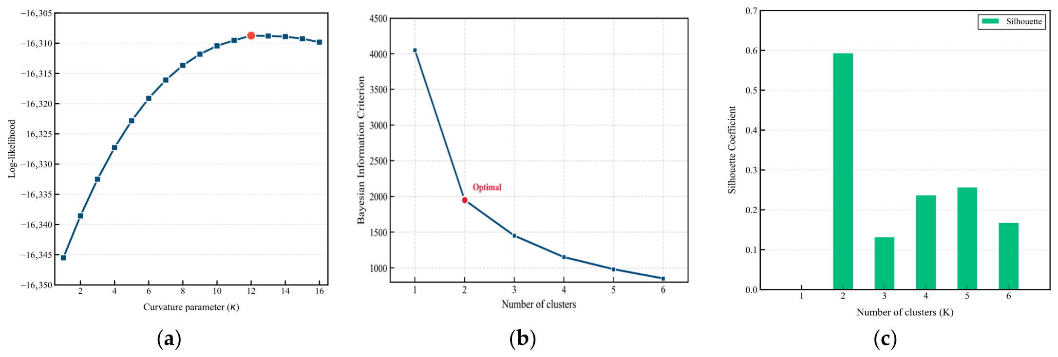
The curvature coefficient, $\kappa$, controls the nonlinear sensitivity of perceived delay risk to the delay-to-RCT ratio, so it is calibrated before the main preference estimation. To avoid strong correlation between $\kappa$ and the marginal utility coefficient ${\beta }_{n,R}$, which may destabilize estimation, this study calibrates $\kappa =\{1,2,3,\dots ,16\}$ through grid search and then treats it as fixed in the main model. As shown in Figure 1a, model fit is optimized when $\kappa =12$. The optimal number of passenger classes is then evaluated using the Bayesian information criterion (BIC) and silhouette coefficient, as shown in Figure 1b and Figure 1c, respectively. Considering these evaluation results, $K$ = 2 is selected as the optimal number of passenger classes.

The full-sample preference model estimation results are presented in

Table 4. Full-sample preference model estimation results.

Parameter Dimension	Variable	Value	z-stat
Constant	eVTOL constant	1.6880	14.19 ***
Constant	Taxi/ride-hailing constant	0.6940	8.09 ***
Random parameter mean	$\mathrm{Cos}\mathrm{t} \mathrm{coefficient}, {\beta }_c$	−0.3600	−4.36 ***
Random parameter mean	$\mathrm{Time} \mathrm{coefficient}, {\beta }_t$	−2.2749	−11.81 ***
Random parameter mean	Delay-risk-perception coefficient, ${\beta }_R$	−3.5170	−17.38 ***
Random parameter standard deviation	${\sigma }_c$	1.0400	11.99 ***
Random parameter standard deviation	${\sigma }_t$	1.8692	9.31 ***
Random parameter standard deviation	${\sigma }_R$	1.4145	10.24 ***
Nested structure parameter	${\lambda }_e$	0.5090	-
Nested structure parameter	${\lambda }_g$	1	-
Overall fit	Log-likelihood (LL)	−9624.6581	-
Overall fit	Akaike information criterion (AIC)	19,267.3161	-
Overall fit	Bayesian information criterion (BIC)	19,304.6138	-
Overall fit	${\rho }^2$	0.1723	-

Note: z-stat denotes the z-statistic. The inclusive value parameter of the ground transport nest, ${\lambda }_g$, is fixed at 1 as the normalization benchmark, and the eVTOL nest parameter, ${\lambda }_e$, is estimated relative to this benchmark. Triple asterisks (***) indicate significance at the 1% level.

. The main model provides a satisfactory fit and explains mode-choice behavior in this scenario. The mean coefficients on cost, travel time, and delay-risk perception are all significantly negative at the 1% level, indicating that higher feeder cost, longer travel time, and stronger delay-risk perception all reduce passenger utility. The value of ${\rho }^2=0.1723$ is acceptable for discrete-choice models in transport applications.

The standard-deviation parameters are also highly significant, indicating substantial unobserved heterogeneity in time valuation and delay-risk perception under inter-hub transfer constraints. To identify latent behavioral groups, individual posterior preference parameters are extracted and clustered using a Gaussian mixture model (GMM) [40]. Candidate class numbers are set as $G=1,\dots ,6$, and the Bayesian information criterion (BIC) and silhouette coefficient are used for evaluation [41]. Although BIC declines as $G$ increases, the decline shows a clear elbow at $G=2$. The silhouette coefficient also reaches its maximum at $G=2$, indicating the best statistical separation. The final classification therefore uses two classes.

The modeling choices follow the estimation evidence. The delay-risk curvature is calibrated before the main preference estimation to avoid confounding it with the delay-risk coefficient. The two passenger classes are retained because the BIC and silhouette results jointly support a two-class solution. Their labels are interpreted using the estimated value of time, willingness to pay for delay-risk reduction, and scenario-specific eVTOL shares. The nested-logit structure relaxes the independence-of-irrelevant-alternatives assumption within each feeder nest while retaining a parsimonious specification for the corridor study.

These behavioral choices are fixed when the lower-level SUE is embedded in the scheduling model. This separation keeps the preference-estimation assumptions explicit while allowing passenger response to remain endogenous to the operator’s service supply.

The specific estimates for $G=2$ are shown in

Table 5. Class-specific model estimation results.

Passenger Class	Indicator	Class 1	Class 2
Class profile	Market share	18.03%	81.97%
Utility parameter	$AS{C}_E$	0.2446 (0.77)	1.3012 *** (8.66)
Utility parameter	$AS{C}_{Taxi}$	−0.7705 *** (−3.08)	0.4398 *** (4.53)
Utility parameter	${\beta }_c$	−0.0074 *** (−6.82)	−0.0071 *** (−15.48)
Utility parameter	${\beta }_t$	−0.0205 *** (−4.15)	−0.0065 ** (−2.34)
Utility parameter	Delay-risk-perception coefficient, ${\beta }_R$	−0.0975 *** (−7.00)	−0.0331 *** (−6.76)
Behavioral indicator	Value of time (VOT)	165.10	55.26
Behavioral indicator	Willingness to pay for delay-risk reduction (WTP)	13.11	4.68
eVTOL share	Relaxed scenario (120 min)	49.21%	35.34%
eVTOL share	Critical scenario (90 min)	54.17%	48.43%
eVTOL share	Urgent scenario (75 min)	53.17%	75.57%

Note: The base mode is airport express rail. Triple asterisks (***) and double asterisks (**) indicate significance at the 1% and 5% levels, respectively. Values in parentheses are z-statistics.

.

The two classes exhibit significant preference heterogeneity under remaining connection time constraints. Their cost coefficients are close, suggesting that, in inter-hub transfer scenarios, the main difference lies in the strength of their sensitivity to travel time and delay-risk perception.

Class 1 accounts for 18.03% of the sample. Its behavioral parameters show stronger negative sensitivity to travel time and delay-risk perception. Its value of time and willingness to pay for unit delay-risk reduction are also higher than those of Class 2. Its $AS{C}_E$ is statistically insignificant, suggesting no clear additional intrinsic preference for eVTOL after controlling for cost, travel time, and delay-risk perception. When RCT is reduced from 120 min to 75 min, the eVTOL choice share for this class remains close to 50%. Given its high time value and WTP for delay-risk reduction, this group places greater weight on reducing time loss and delay-related disutility. We therefore label Class 1 as “robustness-oriented passengers”.

Class 2 accounts for 81.97% of the sample. It has lower value of time and lower willingness to pay for delay-risk reduction, but its $AS{C}_E$ is statistically significant, indicating a latent acceptance of eVTOL as a new transport mode. When RCT is reduced from 120 min to 75 min, its eVTOL choice share increases from 35.34% to 75.57%. This class is therefore more sensitive to tightening time constraints and more likely to switch to eVTOL under urgency. We label Class 2 as “general passengers”.

2.2. Bilevel Planning Model Considering Heterogeneous Passenger Behavior

The eVTOL operation schedule is formulated as a bilevel network design problem under a leader–follower structure.

This structure reflects a planning-stage supply-response process in which the operator first designs the eVTOL service supply and passengers then respond to the available service options. In the upper level, the operator selects feasible eVTOL operation paths and schedules subject to the given fleet and infrastructure capacities. In the lower level, passengers choose among available modes and flights according to heterogeneous preferences, resulting in a stochastic user equilibrium passenger-flow assignment [42,43]. The resulting passenger allocation determines realized ridership, system resource use, and operator revenue.

2.2.1. Physical Scenario

The planning horizon, $\mathcal{T}$, is discretized into equal time steps, $\Delta t$, where $\Delta t=1$ min. On the supply side, the system operates a homogeneous eVTOL fleet subject to onboard state of charge (SOC), finite take-off/landing resources, and finite charging-pile capacity [8,10,44]. On the demand side, the model represents time-varying bidirectional feeder demand between a pair of hubs. Upon entering the decision stage at the origin hub, each passenger chooses between operator-provided eVTOL service and external transport under a given remaining connection time.

Physical feasibility is enforced through energy continuity, charging duration, and take-off/landing separation. Each flight task, $l$, between two hubs is assumed to have fixed flight time and fixed energy consumption, $E_l^{flight}$. The remaining energy, $E_p(t)$, of the aircraft executing path $p$ at time $t$ must remain within the admissible battery operating range [8,10]:

$$E_{min}\le E_p(t)\le E_{max}$$

(6)

In the numerical experiments, $E_{min}=28$ kWh and $E_{max}=140$ kWh, corresponding to a 20% minimum SOC threshold. If the projected energy after the next flight falls below $E_{min}$, the aircraft must charge before executing that flight [10]. Otherwise, charging can be scheduled as needed. Each charging operation restores the battery to $E_{max}$, and the charging duration, $\Delta T_c$, depends on the current remaining energy [8,44]:

$$\Delta T_c=⌈60\cdot {\displaystyle \frac{E_{max}-E_p(t)}{P_{max}}}⌉$$

(7)

where $P_{max}$ is the constant charging power. Because $\Delta T_c$ is measured in minutes and $P_{max}$ is specified in kW, Equation (7) uses the minute-based conversion of the charging time. In the time–space state network, this corresponds to a charging arc from $(h,t,e)$ to $(h,t+\Delta T_c,E_{\max })$.

For two consecutive operations, $o$ and o′, using the same take-off/landing resource, the minimum separation requirement is [10,45]:

$$|t_o^{op}-t_{o^{\prime }}^{op}|\ge T_s$$

(8)

Given the discrete time step, $\Delta t$, the take-off/landing resource capacity of hub $h$, $C_h^{run}$, is as follows:

$$C_h^{run}=⌊{\displaystyle \frac{\Delta t}{T_s}}⌋$$

(9)

where the floor operator ensures that only complete take-off/landing operations are counted within each discrete time step.

2.2.2. Time–Space State Network

The time–space state network is defined as a directed acyclic graph, $\mathcal{G}=(\mathcal{N},\mathcal{A})$. The node set $\mathcal{N}$ contains nodes $v=(h,t,e)$, where $h\in \mathcal{H}$ denotes a physical hub, $t\in \mathcal{T}$ denotes a discrete time, and $e$ denotes battery state of charge. The directed arc set $\mathcal{A}$ contains operation arcs and service arcs.

Operation arcs, ${\mathcal{A}}_{phys}$, represent eVTOL circulation and energy transition, including flight, turnaround, charging, and parking arcs. A flight arc, ${\mathcal{A}}_{fly}$, connects $(h_i,t,e)$ to $(h_j,t+t_l,e-E_l^{flight})$, representing spatial displacement, time progression, and energy consumption during a flight task. A turnaround arc, ${\mathcal{A}}_{turn}$, connects $(h,t,e)$ to $(h,t+T_{turn},e)$, representing mandatory ground time for boarding, alighting, equipment cooling, and safety checks. A charging arc, ${\mathcal{A}}_{chg}$, connects $(h,t,e)$ to $(h,t+\Delta T_c,t,e+E_{max})$ charging and captures energy replenishment over one time step. A parking arc, ${\mathcal{A}}_{staypark}$, connects $(h,t,e)$ to $(h,t+\Delta t,e)$, representing idle waiting without energy change.

Service arcs, ${\mathcal{A}}_{serv}$, describe travel choices by heterogeneous passengers in the time–space network, including flight service arcs, external transport arcs, and waiting arcs. A flight service arc, ${\mathcal{A}}_F$, connects $(h_i,t)$ to $(h_j,t+t_l)$ and corresponds to a flight arc, ${\mathcal{A}}_{fly}$, selected by the upper-level decision. An external transport arc, ${\mathcal{A}}_X$, connects $(h_i,t)$ to $(h_j,t+{\tau }_{travel}^m)$, representing completion of the hub transfer by an external mode. A waiting arc, ${\mathcal{A}}_{wait}$, connects $(h,t)$ to $(h,t+\Delta t)$, representing time spent waiting inside a hub.

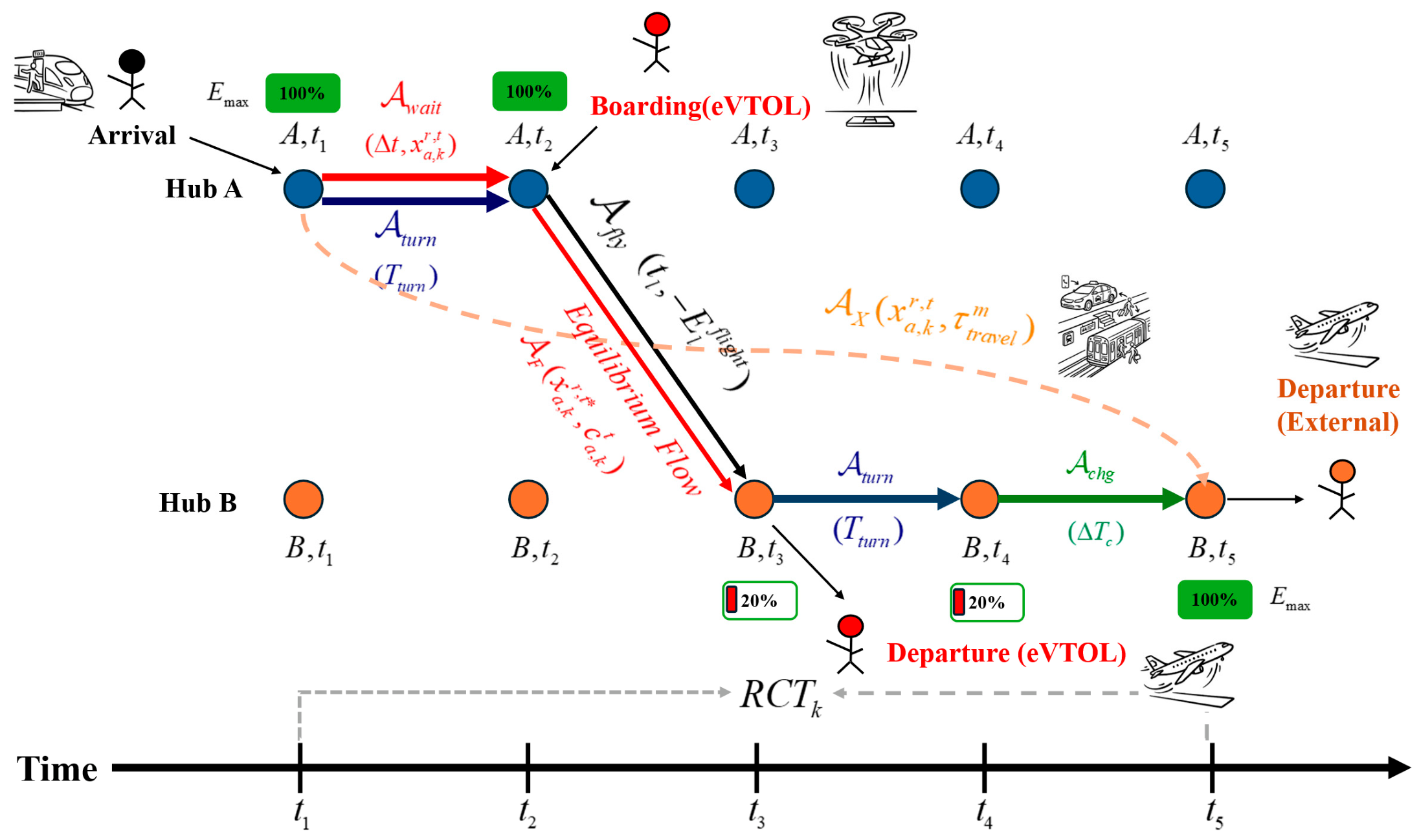
Figure 2 illustrates the operation process of a single eVTOL and the passenger travel-choice process in the time–space network. An eVTOL with initial full energy, $E_{max}$, enters the turnaround arc, ${\mathcal{A}}_{turn}$, at hub A at time $t_1$ and completes ground turnaround in $T_{turn}$. It then follows a flight arc, ${\mathcal{A}}_{fly}$; flies for $t_l$; consumes $-E_l^{flight}$; and arrives at hub B at time $t_3$. After landing, it enters a charging arc, ${\mathcal{A}}_{chg}$, $\Delta T_c$ and reaches SOC $e^{\prime }$ at time $t_4$. If no task is assigned, the aircraft remains on a parking arc, ${\mathcal{A}}_{park}$.

Passenger choices occur on service arcs, ${\mathcal{A}}_{serv}$. Passengers arriving at hub A at $t_1$ choose a feeder mode under the remaining connection time condition, $RC{T}_k(t)$. If they choose eVTOL, they first spend waiting time on ${\mathcal{A}}_{wait}$, board at node $(A,t_2)$, and then travel on an eVTOL flight service arc in ${\mathcal{A}}_F$. If they choose external transport, they directly take external transport arc ${\mathcal{A}}_X$ to hub B and complete the hub transfer process. They then proceed through common downstream processes, such as security screening and boarding. The labels $x_{a,k}^{r,t*}$ and $c_{a,k}^t$ on eVTOL flight service arcs denote equilibrium passenger flows and perceived impedance solved by the SUE model in Section 2.2.4. Finally, eVTOL passenger flow and external transport flow exit the network at nodes $(B,t_3)$ and $(B,t_5)$, respectively.

2.2.3. Model Assumptions and Notation

Four assumptions are introduced to keep the model tractable. First, the eVTOL operation plan is fixed over the planning horizon and does not include real-time rolling adjustment. Fleet size, take-off/landing resources, and charging facilities remain fixed. Second, passenger demand is aggregated by class. Passengers in the same class share utility parameters, and class differences are represented by cost, travel-time, and delay-risk-perception coefficients. Third, all feeder demand generated during the planning horizon must be assigned to a service. Demand cancellation, trip abandonment, and unserved demand are not considered. Fourth, external transport modes do not participate in the operation optimization. Their cost, travel time, waiting time, and potential delay are exogenously given. Taxi/ride-hailing and airport express rail are used as the external transport alternatives.

Table 6. Notation for the bilevel planning model.

Symbol	Description
$\mathcal{T}$	Set of discrete time steps
$\mathcal{H}$	Set of hub nodes
$\mathcal{K}$	Set of passenger classes
$\mathcal{P}$	Set of candidate operation paths
$\mathcal{M}$	Set of external transport modes
$\mathcal{N}$	Set of time–space network nodes
$\mathcal{A}$	Set of directed arcs in the time–space network
${\mathcal{A}}_F,{\mathcal{A}}_X$	Sets of eVTOL service arcs and external transport arcs
$N_{ac}$	Upper bound on total fleet size
$S,S_a(z)$	Single eVTOL capacity and available capacity of flight service arc $a$
$C_h^{run},C_h^{chg}$	Take-off/landing resource capacity and charging-pile capacity
$u_{h,t,p}^{run},u_{h,t,p}^{chg}$	Take-off/landing and charging resource occupation parameters
${\xi }_{a,p}$	Association parameter between service arc and operation path
$E_p$	Total energy consumption of operation path $p$
$D_{r,k}^t$	Demand of passenger class $k$ on route $r$ at time $t$
$Q_{r,k,b}$	Total demand in peak period $b$
$d_l,d_m$	Potential delay of eVTOL flight $l$ and external mode $m$
${\mu }_b,{\sigma }_b$	Peak mean time and time span
$RC{T}_k(t)$	Remaining connection time of passenger class $k$ at decision time $t$
$AS{C}_E,AS{C}_m$	Alternative-specific constants for eVTOL and external modes
$\kappa$	Curvature coefficient in the delay-risk-perception function
${\beta }_{k,c},{\beta }_{k,t},{\beta }_{k,R}$	Cost, time, and delay-risk-perception coefficients
${\eta }_k$	Upper nest scale parameter
${\mu }_{E,k},{\mu }_{X,k}$	Within-nest scale parameters for eVTOL and external nests
$F_E,F_m$	eVTOL fare and external transport fare
$C_{fix},C_{inf}$	Fleet and charging-infrastructure fixed costs
$C_{ops},C_{land},c_{elec}$	Flight-time operating cost, landing cost, and electricity price
$c_p^{var}$	Variable operating cost of path $p$
$z_p$	Binary path operation variable
$x_{a,k}^{r,t}$	Microscopic assignment flow on arc $a$
$f_{\omega ,k}^{r,t}$	Passenger service-path flow
$y_{k,r}^{E,t},y_{k,r}^{X,t}$	Aggregate flows in eVTOL and external nests
$q_{v,k}^{r,t}$	Net node flow
$c_{a,k}^t$	Generalized arc impedance
${\gamma }_a$	Shadow price of the capacity constraint

summarizes the main sets, parameters, and decision variables used in the model. Symbols not listed in the table are defined in the text.

2.2.4. Lower-Level Model

The lower-level model is a capacity-constrained stochastic user equilibrium problem. It describes how heterogeneous passengers choose paths in the time–space network according to travel utility under a given upper-level flight supply, and how these choices lead to an equilibrium flow distribution.

The demand density, $D_{r,k}^t$, for passenger class $k$ on route $r$ is assumed to follow a two-peak Gaussian model:

$$D_{r,k}^t={\displaystyle \sum _{b\in \{1,2\}}\frac{Q_{r,k,b}}{\sqrt{2\pi }{\sigma }_b}}\exp \left(-{\displaystyle \frac{{(t-{\mu }_b)}^2}{2{\sigma }_b^2}}\right)$$

(10)

where $Q_{r,k,b}$ is the total demand in peak period $b$, and ${\mu }_b$ and ${\sigma }_b$ denote the mean peak time and time-coverage span. During hub transfer, each passenger faces a clear remaining connection time. In the dynamic assignment model, $RC{T}_k(t)$ denotes the remaining time budget of passenger class $k$ at decision time $t$, updated from the SP scenario-level $RC{T}_s$ according to the current decision time. This dynamic RCT enters the delay-risk-perception function and affects passengers’ perceived utility at each decision time.

The lower-level model uses the utility structure calibrated in Section 2.1 and converts individual preference parameters into class-specific parameters. For passenger class $k$, the utility of choosing eVTOL flight $l$ at time $t$ is as follows:

$$V_{k,l}^E(t)=AS{C}_E+{\beta }_{k,c}{F}_E+{\beta }_{k,t}(t_{arr}^l-t)+{\beta }_{k,R}{R}_{k,l}(t)$$

(11)

where $AS{C}_E$ is the eVTOL alternative-specific constant; $F_E$ is the fixed fare; $t_{arr}^l-t$ is the total travel time, including waiting and flight time; and $R_{k,l}(t)$ is the delay-risk-perception function under the passenger’s remaining connection time constraint.

According to Equation (5), the delay-risk-perception term is as follows:

$$R_{k,l}(t)=\exp \left(\kappa \cdot {\displaystyle \frac{d_l}{RC{T}_k(t)}}\right)-1$$

(12)

where $d_l$ is the potential delay of eVTOL flight $l$, $RC{T}_k(t)$ is the remaining connection time of passenger class $k$ at decision time $t$, and $\kappa$ is the curvature coefficient.

For external transport mode, $m$, the utility function is similarly defined as follows:

$$V_{k,m}^X(t)=AS{C}_m+{\beta }_{k,c}{F}_m+{\beta }_{k,t}({\tau }_{travel}^m+{\tau }_{wait}^m(t))+{\beta }_{k,R}{R}_{k,m}(t)$$

(13)

where $AS{C}_m$ is the constant of external transport mode, $m$; ${\tau }_{travel}^m$ is its base deterministic travel time; ${\tau }_{wait}^m(t)$ is the waiting time at time $t$; and the dynamic delay-risk-perception term is $R_{k,m}(t)=\exp \left(\kappa \cdot {\displaystyle \frac{d_m}{RC{T}_k(t)}}\right)-1$, where $d_m$ is the potential delay of mode $m$.

The generalized utilities are transformed into generalized arc impedances in the time–space graph. For an eVTOL service arc, $a$, whose corresponding flight is $l(a)$, impedance is defined as the negative of utility, $c_{a,k}^{E,t}=-V_{k,l(a)}^E(t)$. For an external transport arc, $a$, whose corresponding external mode is $m(a)$, impedance is $c_{a,k}^{X,t}=-V_{k,m(a)}^X(t)$.

Based on these generalized arc impedances, the lower-level model uses a nested logit SUE form to describe path assignment by heterogeneous passengers in the time–space service network. Let ${\Omega }_{r,t}$ denote the feasible service-path set for route $r$ and departure time $t$, partitioned into the eVTOL flight nest, ${\Omega }_{E,r,t}$, and the ground transport nest, ${\Omega }_{X,r,t}$. ${\eta }_k$ is the nest-level scale parameter for passenger class $k$, while ${\mu }_{E,k}$ and ${\mu }_{X,k}$ are the within-nest path-choice scale parameters. In the numerical experiments, ${\eta }_k$ is normalized to 1, and the within-nest scales are derived from the full-sample inclusive-value parameters as ${\mu }_{E,k}=1/{\lambda }_e=1.965$ and ${\mu }_{X,k}=1/{\lambda }_g=1$.

Following Sheffi’s equivalent mathematical programming approach, under a given upper-level schedule and its resulting flight capacity, the flow distribution of the nested logit SUE model is the optimal solution of the following capacity-constrained convex optimization problem (P1). The probabilistic equilibrium assignment can be expressed through an entropy-optimization form [26,43]. The derivation is given in Appendix A.

$$(P1)\hspace{1em}{\min }_{x,f,y}Z(x,f,y)={\displaystyle \sum _{a\in \mathcal{A}}{\displaystyle \sum _{k\in \mathcal{K}}{\displaystyle \sum _{r,t}{x}_{a,k}^{r,t}}}}{c}_{a,k}^t+{\Psi }_{ent}(f_k^t,y_k^t)$$

(14)

The first term is the generalized total system impedance, representing the cumulative product of arc flow $x_{a,k}^{r,t}$ and corresponding arc impedance $c_{a,k}^t$ over all passengers in the time–space network. ${\Psi }_{ent}$ contains the generalized entropy function with microscopic choice entropy and nested-structure correction:

$$\begin{array}{l}{\Psi }_{ent}(f_k,y_k)={\displaystyle \sum _{r,t}[}{\displaystyle \frac{1}{{\mu }_{E,k}}}\mathcal{H}(f_E^t)+{\displaystyle \frac{1}{{\mu }_{X,k}}}\mathcal{H}(f_X^t)\\ +\left({\displaystyle \frac{1}{{\eta }_k}}-{\displaystyle \frac{1}{{\mu }_{E,k}}}\right)\mathcal{H}(y_E^t)+\left({\displaystyle \frac{1}{{\eta }_k}}-{\displaystyle \frac{1}{{\mu }_{X,k}}}\right)\mathcal{H}(y_X^t)]\end{array}$$

(15)

where $\mathcal{H}(x)={\displaystyle \sum x_j}\ln x_j$ is the entropy operator. $y_{k,r}^{E,t}$ and $y_{k,r}^{X,t}$ are the eVTOL-nest and ground-transport-nest flows for passenger class $k$ on route $r$ at time $t$. Under this scale setting, the entropy coefficients are non-negative, and the lower-level equivalent program remains convex.

Let $f_{\omega ,k}^{r,t}$ denote the assignment flow of passenger class $k$ on path $\omega$. Arc flows and nest aggregate flows are obtained from path flows:

$$x_{a,k}^{r,t}={\displaystyle \sum _{\omega \in {\Omega }_{r,t}:a\in \omega }{f}_{\omega ,k}^{r,t}},\hspace{1em}\forall a,k,r,t$$

(16)

$$y_{k,r}^{E,t}={\displaystyle \sum _{\omega \in {\Omega }_{E,r,t}}{f}_{\omega ,k}^{r,t}},\hspace{1em}{y}_{k,r}^{X,t}={\displaystyle \sum _{\omega \in {\Omega }_{X,r,t}}{f}_{\omega ,k}^{r,t}},\hspace{1em}\forall k,r,t$$

(17)

Given an upper-level schedule, $z$, the available seat capacity of eVTOL flight service arc $a$ is determined by the selected operation paths:

$$S_a(z)=S{\displaystyle \sum _{p\in \mathcal{P}}{\xi }_{a,p}}{z}_p,\hspace{1em}\forall a\in {\mathcal{A}}_F$$

(18)

The model constraints are as follows:

$${\displaystyle \sum _{w:(v,w)\in \mathcal{A}}{x}_{vw,k}^{r,t}}-{\displaystyle \sum _{w:(w,v)\in \mathcal{A}}{x}_{wv,k}^{r,t}}=q_{v,k}^{r,t},\hspace{1em}\forall v\in \mathcal{N},k\in \mathcal{K},r,t$$

(19)

$$y_{k,r}^{E,t}+y_{k,r}^{X,t}=D_{r,k}^t,\hspace{1em}\forall k,r,t$$

(20)

$${\displaystyle \sum _{k\in \mathcal{K}}{\displaystyle \sum _{r,t}{x}_{a,k}^{r,t}}}\le S_a(z),\hspace{1em}\forall a\in {\mathcal{A}}_F$$

(21)

$$x_{a,k}^{r,t}\ge 0,\hspace{1em}{f}_{\omega ,k}^{r,t}\ge 0,\hspace{1em}{y}_{k,r}^{E,t}\ge 0,\hspace{1em}{y}_{k,r}^{X,t}\ge 0$$

(22)

Equations (16) and (17) aggregate path flows into service-arc flows and nest flows, and Equation (18) gives the available capacity of flight service arcs under a given upper-level schedule. Equation (19) is the flow-conservation constraint, where $q_{v,k}^{r,t}$ equals $D_{r,k}^t$ at the origin node, $-D_{r,k}^t$ at the destination node, and 0 at intermediate nodes. Equation (20) assigns all demand to either the eVTOL nest or the ground transport nest, while Equation (21) ensures that passenger flow on eVTOL service arc $a$ does not exceed its available capacity, $S_a(z)$. The dual variable ${\gamma }_a\ge 0$ represents the shadow price of capacity scarcity: ${\gamma }_a=0$ when capacity is slack and ${\gamma }_a>0$ when the capacity constraint is binding. Solving the KKT conditions of this convex program, as shown in Appendix A, proves its equivalence to the capacity-constrained nested logit SUE. Equation (22) imposes non-negativity [43].

2.2.5. Upper-Level Model

The upper-level model selects candidate eVTOL operation paths through the binary variables, $z_p$, thereby determining the flight schedule under the specified fleet, infrastructure, and fare configuration. The objective is operator profit maximization. $z_p\in \{0,1\}$, and $p\in \mathcal{P}$. $z_p=1$ indicates that candidate operation path $p$ is selected, and $z_p=0$ otherwise.

The infrastructure fixed cost, $C_{fixed}$, including fleet depreciation and charging-pile construction, is as follows:

$$C_{fixed}=C_{fix}{N}_{ac}+C_{inf}{\displaystyle \sum _{h\in \mathcal{H}}{C}_h^{chg}}$$

(23)

The variable cost, $C_{var}(z)$, associated with the operation plan includes flight operating cost and electricity consumption cost. $c_p^{var}$ contains maintenance cost corresponding to flight operating time and the take-off-and-landing cycle cost of each flight leg:

$$c_p^{var}={\displaystyle \sum _{l\in p}(C_{ops}{t}_l+C_{land})}$$

(24)

where $C_{ops}$ is the operating cost per unit flight time, $C_{land}$ is the cost per take-off or landing, and $t_l$ is the duration of a single flight.

$$C_{var}(z)={\displaystyle \sum _{p\in \mathcal{P}}{z}_p}(c_p^{var}+c_{elec}{E}_p)$$

(25)

where $c_{elec}$ is the unit electricity price, and $E_p$ is the total energy consumption of path $p$.

Total revenue is determined by the actual flow assigned to each eVTOL flight service arc, $x_{a,k}^{r,t*}$, fed back by the lower-level model, multiplied by the fare. Operator profit $\Pi (z)$ is as follows:

$${\max }_z\hspace{1em}\Pi ={\displaystyle \sum _{a\in {\mathcal{A}}_F}{\displaystyle \sum _{k\in \mathcal{K}}{\displaystyle \sum _{r,t}{F}_E}}}{x}_{a,k}^{r,t*}(z)-\left(C_{fixed}+C_{var}(z)\right)$$

(26)

The total number of eVTOLs put into operation cannot exceed the operator’s fleet size:

$${\displaystyle \sum _{p\in \mathcal{P}}{z}_p}\le N_{ac}$$

(27)

For any hub, $h$, and discrete time, $t$, the total resource occupation of all selected paths cannot exceed the physical capacity of the hub. The take-off/landing resource and charging-pile constraints are as follows:

$${\displaystyle \sum _{p\in \mathcal{P}}{u}_{h,t,p}^{run}}{z}_p\le C_h^{run},\hspace{1em}\forall h\in \mathcal{H},t\in \mathcal{T}$$

(28)

$${\displaystyle \sum _{p\in \mathcal{P}}{u}_{h,t,p}^{chg}}{z}_p\le C_h^{chg},\hspace{1em}\forall h\in \mathcal{H},t\in \mathcal{T}$$

(29)

where $u_{h,t,p}^{run}\in \{0,1\}$ and $u_{h,t,p}^{chg}\in \{0,1\}$ are time–space occupation indicators for take-off/landing and charging resources, respectively. They indicate whether candidate operation path $p$ occupies the corresponding facility at hub $h$ at time $t$. $C_h^{run}$ and $C_h^{chg}$ are the corresponding capacity limits.

2.2.6. Social Net Utility of the Feeder System

Beyond maximizing operator profit at the upper level, this study defines the social net utility of the feeder system to evaluate the combined effect of eVTOL entry on operator profit and monetized passenger-utility improvement. This measure focuses on the internal economic and passenger-utility effects of the feeder system and should not be interpreted as a complete social-welfare measure. Broader externalities, such as emissions, noise, land-use impacts, and other wider social effects, are outside the present indicator. In the no-eVTOL scenario, passengers can only complete inter-hub transfer by external transport modes. For travel by passenger class k on service arc a, the evaluation impedance is defined as follows:

$${\overline{c}}_{a,k}^{eval}=-\left({\beta }_{k,t}{T}_a+{\beta }_{k,c}{F}_a+{\beta }_{k,R}{R}_a\right),\hspace{1em}a\in {\mathcal{A}}_{serv}, k\in \mathcal{K}$$

(30)

where ${\overline{c}}_{a,k}^{eval}$ is the service-arc impedance used for social net utility evaluation, ${\mathcal{A}}_{serv}$ is the set of service arcs, and $F_a$ is the travel cost associated with arc $\mathit{a}$.

Let $G_k^E$ denote the equilibrium evaluation impedance of passenger class $k$ with eVTOL entry, and let $G_k^0$ denote the corresponding impedance without eVTOL entry. The monetized passenger welfare increment is as follows:

$$\Delta C{S}^{eval}={\displaystyle \sum _{k\in \mathcal{K}}\frac{G_k^0-G_k^E}{-{\beta }_{k,c}}}$$

(31)

The social net utility of the feeder system is then the sum of operator profit and monetized passenger welfare increment.

Because the passenger welfare increment is expressed in CNY-equivalent units using the estimated marginal utility of cost in Equation (31), it can be combined with operator profit. The resulting indicator captures operator return and passenger-utility improvement within the model, rather than complete social welfare, and is defined as follows:

$$\Delta SW=\Pi (z)+\Delta C{S}^{eval}$$

(32)

2.3. Neur2BiLO-GBD Hybrid Solution Framework

Directly solving the eVTOL scheduling problem with stochastic user equilibrium response is difficult for two reasons. First, the problem includes both 0–1 scheduling decisions and nested logit SUE response, creating substantial combinatorial and nonlinear complexity. Second, the lower-level model contains a highly nonlinear equivalent objective with logarithmic entropy terms, so it is not directly amenable to KKT-based linearization. Although generalized Benders decomposition (GBD) is advantageous for high-dimensional discrete optimization, it does not, by itself, reformulate or solve the original nonlinear bilevel model [33,34].

The Neur2BiLO value-function reformulation first produces a surrogate master problem. GBD then corrects the nonlinear entropy component through iterative cuts, and the passenger response for the selected schedule is obtained by re-solving the original lower-level SUE model.

To address these difficulties, this study proposes a generalized Benders decomposition algorithm based on Neur2BiLO, referred to as Neur2BiLO-GBD. The method embeds a neural approximation of the lower-level optimal value function into a single-level surrogate model [31]. It then decomposes the model into a surrogate master problem and a relaxed subproblem, and it finally re-solves the original lower-level SUE under the selected schedule to recover the original-model SUE response.

2.3.1. Single-Level Reformulation Based on Neur2BiLO

The original bilevel model can be written as follows:

$${\max }_{z,v}\hspace{1em}\Pi (z,v)=Rev(v)-\left(C_{fixed}+C_{var}(z)\right)$$

(33)

$$\mathrm{s}.\mathrm{t}.\hspace{1em}z\in \mathcal{Z}$$

(34)

$$\hspace{1em}v\in \arg {\min }_{v^{\prime }\in {\Omega }_{LL}(z)}Z(v^{\prime })$$

(35)

where $z$ is the upper-level scheduling decision vector; $v=(x,f,y)$ is the lower-level passenger-flow assignment vector; and $\Pi (z,v)$ is operator profit, determined by eVTOL fare revenue, $Rev(v)$, and operating cost, $C_{fixed}+C_{var}(z)$. $\mathcal{Z}$ is the feasible region of the upper-level physical and logical scheduling constraints. ${\Omega }_{LL}(z)$ is the feasible region of lower-level passenger-flow variables under a given schedule, including flow conservation, demand satisfaction, capacity limits, and non-negativity. $Z(v)$ is the equivalent objective of the lower-level nested logit SUE.

Following the value-function reformulation principle proposed by Dumouchelle et al. under the optimistic assumption, the lower-level optimal value function is defined as follows:

$$\Phi (z)={\min }_{v^{\prime }\in {\Omega }_{LL}(z)}Z(v^{\prime })$$

(36)

Based on this value function, the bilevel model can be rewritten as follows:

$${\max }_{z\in \mathcal{Z},v\in {\Omega }_{LL}(z)}\hspace{1em}Rev(v)-\left(C_{fixed}+C_{var}(z)\right)$$

(37)

$$\mathrm{s}.\mathrm{t}.\hspace{1em}Z(v)\le \Phi (z)$$

(38)

Here, $\Phi (z)$ is the optimal value of the lower-level problem under schedule $z$. Directly computing $\Phi (z)$ requires repeatedly solving the dynamic SUE problem during combinatorial search, which is computationally expensive. This study therefore uses a multilayer perceptron (MLP) with ReLU activation as the value-function approximation, denoted as $\widehat{\Phi }(z;\theta )$. The surrogate model estimates the lower-level equilibrium value under a given schedule, using scheduling variables as inputs and lower-level SUE objective values as targets. The training samples, network settings, and prediction accuracy are reported in Section 3.2. Following Fischetti and Jo, the forward pass of a ReLU neural network can be represented exactly, via a Big-M formulation, as standard mixed-integer linear constraints with auxiliary continuous and binary variables [32].

Because neural-network prediction may contain errors, the surrogate may underestimate the true lower-level value, $\widehat{\Phi }(z)<\Phi (z)$. Since $Z(v)$ is always greater than or equal to the true lower bound, $\Phi (z)$, the constraint $Z(v)\le \widehat{\Phi }(z)$ may make the problem infeasible. A non-negative continuous slack variable $s\ge 0$ is therefore introduced, yielding $Z(v)\le \widehat{\Phi }(z)+s$. The upper-level profit objective subtracts a penalty term, $\rho s$, encouraging $s$ to approach 0 and forcing the lower-level objective toward the surrogate optimal boundary, $\widehat{\Phi }$.

The final reconstructed single-level mixed-integer programming model is as follows:

$${\max }_{z\in \mathcal{Z},v\in {\Omega }_{LL}(z),h,b,\widehat{\Phi },s}\hspace{1em}Rev(v)-\left(C_{fixed}+C_{var}(z)\right)-\rho s$$

(39)

$$\mathrm{s}.\mathrm{t}.\hspace{1em}(z,h,b,\widehat{\Phi })\in {\Omega }_{NN}$$

(40)

$$\hspace{1em}Z(v)\le \widehat{\Phi }+s$$

(41)

$$\hspace{1em}s\ge 0$$

(42)

where $h$ and $b$ are auxiliary continuous and binary variables derived from neural-network hidden-layer outputs and activation states; ${\Omega }_{NN}$ denotes the linear polyhedral constraints that represent the forward mapping of the surrogate model; $\rho$ is the neural approximation error penalty coefficient; and $s$ is the slack variable. This reformulation converts the original highly nonlinear nested bilevel model into a single-level mathematical programming model with a value-function constraint.

Solving this single-level model directly with Gurobi remains challenging. First, the constraint $Z(v)\le \widehat{\Phi }(z)+s$ requires the solver to evaluate the lower-level objective, $Z(v)$, inside the optimization model. Because this function contains high-dimensional continuous flow variables and nonlinear logarithmic entropy terms, a MILP solver requires piecewise-linear or outer-approximation representations. Second, these approximations introduce many auxiliary variables and constraints. In a time–space eVTOL network, the number of path-flow, arc-flow, and entropy-related variables grows quickly with the operating duration, making the resulting model difficult to solve.

2.3.2. Surrogate Master Problem and Relaxed Subproblem

To address the dimensional and nonlinear difficulties of direct single-level solution, this section decomposes the model in Section 2.3.1 into a surrogate master problem and a relaxed subproblem. The master problem retains scheduling decisions, linear passenger-flow relations, resource constraints, and neural surrogate constraints, while using an auxiliary variable to represent the nonlinear entropy term in the lower-level SUE equivalent objective. The relaxed subproblem computes the separated entropy value and gradient at candidate points and returns the corresponding linear cuts to the master problem.

The objective, $Z(v)$, in the value-function reformulation constraint can be decomposed into a linear part and a nonlinear entropy term:

$$Z(v)=L(v)+H(v)$$

(43)

where $L(v)$ represents the linear objective term formed by generalized arc impedance and arc flow, and $H(v)$ represents the nonlinear entropy term generated by random utility in the nested logit SUE equivalent form.

The surrogate master problem retains $z$; $v=(x,f,y)$; neural-network linearization variables $h$ and $b$; the value-function prediction, $\widehat{\Phi }$; and slack variable $s$. To avoid explicitly expanding $H(v)$ in the master problem, a continuous variable, $\alpha$, is introduced to represent the entropy term, and its value is progressively approximated by a set of generated cuts, $\mathcal{J}$. The surrogate master problem (MP) is follows:

$${\max }_{z,v,\widehat{\Phi },\alpha ,s,h,b}\hspace{1em}Rev(v)-\left(C_{fixed}+C_{var}(z)\right)-\rho s$$

(44)

$$\mathrm{s}.\mathrm{t}.\hspace{1em}z\in \mathcal{Z}$$

(45)

$$\hspace{1em}v\in {\Omega }_{LL}^{lin}(z)$$

(46)

$$\hspace{1em}(z,h,b,\widehat{\Phi })\in {\Omega }_{NN}$$

(47)

$$\hspace{1em}L(v)+\alpha \le \widehat{\Phi }+s$$

(48)

$$\hspace{1em}\alpha \ge {\mathcal{C}}^{(j)}(v),\hspace{1em}\forall j\in \mathcal{J}$$

(49)

$$\hspace{1em}s\ge 0$$

(50)

where ${\Omega }_{LL}^{lin}(z)$ is the linear feasible region containing flow conservation, path-arc aggregation, demand satisfaction, capacity limits, and non-negativity; $\mathcal{J}$ is the current set of generated entropy cuts; and ${\mathcal{C}}^{(j)}(v)$ is the $j$-th entropy cut. Equation (48) is the value-function reformulation constraint in the master problem, and Equation (49) progressively supplements the separated entropy term through linear cuts.

Additional linear strengthening constraints are added to the surrogate master problem to bound serviceable eVTOL demand, flight capacity, and fare revenue, thereby reducing relaxation errors caused by fractional schedules, capacities, and flows.

The valid inequalities added to the master problem correspond to the lower-level demand satisfaction constraint (20), the flight capacity constraint (21) and the upper-level revenue function (26):

$$0\le {\displaystyle \sum _{a\in {\mathcal{A}}_F}{x}_{a,k}^{r,t}}\le D_{r,k}^t,\hspace{1em}\forall k,r,t$$

(51)

$${\displaystyle \sum _{k\in \mathcal{K}}{\displaystyle \sum _{r,t}{x}_{a,k}^{r,t}}}\le S_a(z),\hspace{1em}\forall a\in {\mathcal{A}}_F$$

(52)

$$Rev(v)={\displaystyle \sum _{a\in {\mathcal{A}}_F}{\displaystyle \sum _{k\in \mathcal{K}}{\displaystyle \sum _{r,t}{F}_E}}}{x}_{a,k}^{r,t}$$

(53)

where $S_a(z)=S{\displaystyle \sum _{p\in \mathcal{P}}{\xi }_{a,p}}{z}_p$ denotes the available capacity generated by schedule $z$ on service arc $a$.

Let the $k$ th candidate point that triggers relaxed-subproblem checking be as follows:

$$(z^k,v^k,{\widehat{\Phi }}^k,{\alpha }^k,s^k)$$

(54)

where $z^k$ is the candidate schedule, $v^k$ is the candidate passenger-flow assignment, ${\widehat{\Phi }}^k=\widehat{\Phi }(z^k;\theta )$ is the neural value-function prediction, ${\alpha }^k$ is the entropy auxiliary variable, and $s^k$ is the slack variable in the value-function reformulation constraint.

The relaxed subproblem fixes candidate passenger flow, $v^k$, and exactly computes the nonlinear entropy term separated from the master problem. The entropy value at the current candidate point is as follows:

$$H^k=H(v^k)$$

(55)

The left-hand side of the complete value-function reformulation constraint is as follows:

$$Z^k=L(v^k)+H^k$$

(56)

where $H^k$ is the nonlinear entropy value corresponding to $v^k$, and $Z^k$ is the full value of $Z(v)$ after adding the entropy term back. If the master-problem auxiliary variable underestimates the true entropy term, that is, if $H^k>{\alpha }^k$, a new entropy cut is generated. To construct this cut, the first-order gradient of the entropy term at the current point is computed as follows:

$$g^k=\nabla H(v^k)$$

(57)

Let $v_i$ denote a component of the passenger-flow vector, $v$. Then,

$$g_i^k={\left.{\displaystyle \frac{\partial H(v)}{\partial v_i}}\right|}_{v=v^k},\hspace{1em}i\in {\mathcal{I}}_v$$

(58)

where ${\mathcal{I}}_v$ is the passenger-flow variable index set, and $g_i^k$ is the partial derivative of the entropy term with respect to $v_i$ at candidate point $k$. The subproblem outputs $H^k$, $Z^k$, and $g^k$, which are used to determine whether a new cut is needed and to construct it.

2.3.3. Linear Cuts and Algorithm Flow

The linear cuts are introduced to tighten the surrogate master problem when the nonlinear entropy term in the lower-level SUE objective is underestimated. In the master problem, this entropy term is represented by an auxiliary variable. For each candidate passenger-flow solution, the relaxed subproblem evaluates the corresponding entropy value and gradient. Because the entropy term is convex with respect to passenger-flow variables, these quantities define the following first-order supporting inequality:

$$H(v)\ge H^k+{(g^k)}^T(v-v^k)$$

(59)

The entropy cut generated at candidate point $k$ is as follows:

$${\mathcal{C}}^{(k)}(v)=H^k+{(g^k)}^T(v-v^k)$$

(60)

When the evaluated entropy value is larger than the auxiliary entropy value at candidate point k, the following linear cut is added to the master problem:

$$\alpha \ge {\mathcal{C}}^{(k)}(v)$$

(61)

Expanding Equation (61) by passenger-flow components gives the following:

$$\alpha \ge H^k-{\displaystyle \sum _{i\in {\mathcal{I}}_v}{g}_i^k}{v}_i^k+{\displaystyle \sum _{i\in {\mathcal{I}}_v}{g}_i^k}{v}_i$$

(62)

As more cuts are added, the auxiliary variable provides a progressively tighter approximation of the entropy term. Consequently, the value-function reformulation constraint in the surrogate master problem becomes closer to that in the original single-level model.

The master-problem decision, $z^{*}$, is based on the neural surrogate approximation of the value function and the iteratively generated linear cuts. After termination, the final $z^{*}$ is substituted back into the original lower-level SUE model to compute the true passenger response, $v^{*}$, and true profit, ${\Pi }_{true}$. This step corrects numerical evaluation bias introduced by surrogate approximation and relaxation. The full procedure is shown in Algorithm 1.

Algorithm 1. Neur2BiLO-GBD solution algorithm
Step	Procedure
Input	Time–space network topology and resource configuration, $\mathcal{G}(\mathcal{N},\mathcal{A});$ passenger origin-destination (OD) demand set and nested logit parameters; pretrained neural surrogate, $\widehat{\Phi }(\mathit{z};\theta )$.
Output	Scheduling decision, ${\mathit{z}}^{\star };$ passenger equilibrium flow assignment, ${\mathit{v}}^{\star };$ true system profit, ${\Pi }_{true}$.
1	Decompose $Z(v)$ as $Z\left(\mathit{v}\right)=L\left(\mathit{v}\right)+H\left(\mathit{v}\right),$ and initialize the entropy cut set $\mathcal{J}$.
2	Repeat.
3	Construct and solve the surrogate master problem MP, including scheduling constraints, linear passenger-flow relations, neural-network surrogate constraints, linear strengthening constraints, and all generated cuts.
4	Obtain candidate point $({\mathit{z}}^k,{\mathit{v}}^k,{\widehat{\Phi }}^k,{\alpha }^k,s^k)$.
5	Fix ${\mathit{v}}^k,$ and compute $H^k=H\left({\mathit{v}}^k\right),$ $Z^k=L\left({\mathit{v}}^k\right)+H^k,$ and ${\mathit{g}}^k=\nabla H\left({\mathit{v}}^k\right)$.
6	If $H^k>{\alpha }^k,$ generate entropy cut ${\mathcal{C}}^{\left(k\right)}\left(\mathit{v}\right)=H^k+\left({\mathit{g}}^k{)}^T\right(\mathit{v}-{\mathit{v}}^k)$ and add it to the master problem.
7	If the current candidate point satisfies the generated-cut conditions, compute candidate profit ${\Pi }^k=Rev\left({\mathit{v}}^k\right)-C_{fixed}-C_{var}\left({\mathit{z}}^k\right)$ and update the incumbent feasible solution.
8	Until the master-problem search terminates, the computational budget is exhausted, or no effective new cut is generated.
9	Fix ${\mathit{z}}^{\star }$ and solve the original lower-level SUE model to obtain true passenger-flow assignment, ${\mathit{v}}^{\star }$.
10	Compute true system profit, ${\Pi }_{true}=Rev\left({\mathit{v}}^{\star }\right)-C_{fixed}-C_{var}\left({\mathit{z}}^{\star }\right)$.
11	Return $({\mathit{z}}^{\star },{\mathit{v}}^{\star },{\Pi }_{true})$.

3. Results and Discussion

3.1. Numerical Experiment Setting

We evaluate the proposed model and solution method using a representative air–rail intermodal feeder scenario between two major hubs. The experiments first compare Neur2BiLO-GBD, Neur2BiLO, mixed-integer Karush–Kuhn–Tucker reformulation (MKKT), and genetic algorithm (GA) benchmarks across problem scales. This comparison evaluates computational efficiency and solution quality. The baseline eVTOL schedule and passenger-flow allocation are then analyzed to illustrate system operation under complex supply–demand conditions. The analysis then examines how fleet size, charging-facility configuration, fare, remaining connection time, and external transport delay affect operator profit and social net utility.

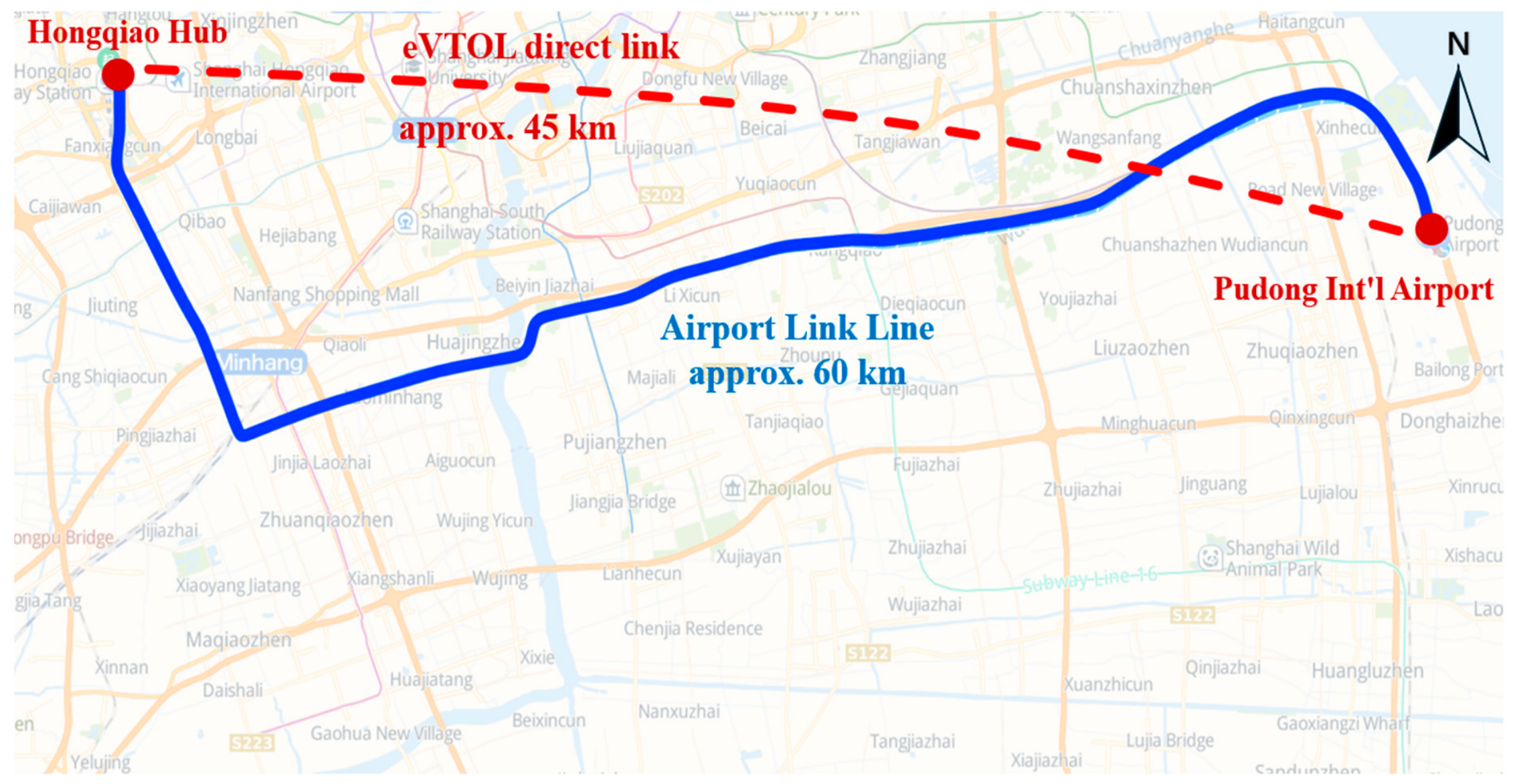
As shown in Figure 3, the case study examines the feeder corridor between Shanghai Hongqiao Integrated Transportation Hub and Pudong International Airport. The straight-line distance is approximately 45 km, and the actual ground feeder distance is approximately 60 km. This corridor represents long-distance dual-hub transfer in a large city. Passenger flow at major transport hubs is strongly concentrated in time and space, making the corridor suitable for inter-hub feeder service [46]. Because current eVTOL operations are constrained by visual flight rules (VFRs) and visual meteorological conditions, safe night operations under low visibility are difficult to ensure. The eVTOL operating window is therefore set to 08:00–18:00 [47].

The numerical parameters include operator supply-side parameters, external-transport parameters, and passenger-behavior parameters. On the supply side, a representative five-seat eVTOL is used to represent a homogeneous fleet. Single-flight duration is set to 14 min, and single-flight energy consumption is set to 30 kWh. The physical and economic parameters used in the optimization are summarized in

Table 7. Physical and economic parameters of the eVTOL fleet.

Category	Parameter	Value	Unit
Physical operation	Rated passenger capacity	5	passengers
Physical operation	Battery energy operating range	[28.0, 140.0]	kWh
Physical operation	Single-flight energy consumption	30.0	kWh
Physical operation	Single-flight duration	14.0	min
Physical operation	Charging power	200.0	kW
Physical operation	Take-off/landing resource capacity	4	operations/min
Physical operation	Ground turnaround time	10.0	min
Economic cost	Daily fixed cost per aircraft	5000	CNY
Economic cost	Daily fixed cost per charging pile	1000	CNY
Economic cost	Electricity price	0.35	CNY/kWh
Economic cost	Cost per take-off-and-landing cycle	150.0	CNY

Note: The baseline configuration uses 16 aircraft, 8 charging piles, 4000 daily transfer passengers, an RCT of 100 min, and an eVTOL fare of 200 CNY. Passenger-behavior coefficients are taken from Table 5, while the physical and economic parameters are used as fixed inputs in the scheduling experiments.

. Passenger-behavior parameters are taken from the estimation results in Section 2.1 and Table 5.

On the demand side, the alternative set is constructed from the travel characteristics of Hongqiao–Pudong-transfer passengers. Existing air–rail intermodal studies show that transfer time, feeder convenience, intermodal passenger behavior, and timetable coordination affect air–rail-connection service quality [48,49,50]. Such passengers usually have high values of time, tight schedule constraints, and luggage, making them sensitive to feeder time and reliability. We therefore exclude conventional urban rail transit from the external alternatives because it is slower, involves more stops, and offers lower comfort. Taxi/ride-hailing and airport express rail are selected as the main external substitutes for eVTOL. Taxi/ride-hailing provides door-to-door feeder service, whereas airport express rail provides a rapid rail feeder connection between Hongqiao Hub and Pudong Airport.

Service and cost parameters for each alternative are set using average road conditions from AutoNavi, historical fare data, and public operating information. In the baseline scenario, taxi/ride-hailing has an average travel time of 60 min, an average waiting time of 5 min, and a fare of 150 CNY. Airport express rail has a travel time of 40 min, an average waiting time of 7.5 min, and a full-trip fare of 26 CNY. These time parameters correspond to the hub transfer process defined in Section 2.1 and exclude common subsequent airport processes. The baseline configuration uses 16 eVTOL aircraft, eight charging piles, 4000 daily passenger trips, RCT = 100 min, and an eVTOL fare of 200 CNY.

The SP design levels and the planning sensitivity settings serve different purposes. The planning experiments decompose running and waiting times and include exploratory values outside the SP attribute ranges, such as the 100-CNY eVTOL fare. Such values are extrapolations of the calibrated utility function rather than additional behavioral observations and should be interpreted as exploratory planning inputs. The 40 min airport-express-rail baseline is a planning input based on corridor operating information, not an SP attribute level, and is therefore treated as an exploratory operational input rather than a new behavioral observation.

The values in Table 7 are representative planning inputs and are not intended as universal platform parameters. They were selected from values commonly used in relevant eVTOL and intermodal-transport studies and from publicly available operating information. The sensitivity analysis varies fleet size, charging capacity, fare, remaining connection time, and external-transport delay, which are the principal planning dimensions examined in the case study. Platform-specific physical and cost inputs remain fixed to define a consistent illustrative operating environment.

The cited studies and public operating information provide the reference context for these representative ranges [8,10,11,12,44,47,48,49,50].

3.2. Algorithm Performance

To evaluate solution performance, this section uses MKKT as the baseline algorithm and compares Neur2BiLO, Neur2BiLO-GBD, and GA across different computational scales. The eVTOL operating durations are 60 min, 120 min, 240 min, 360 min, and 600 min.

All methods use the same baseline configuration, and the time limit for each instance is 600 s. In the experiments, Neur2BiLO-GBD terminates when the solver reaches the time limit, the master-problem search satisfies the solver stopping criterion, or no violated entropy cut is identified at the current candidate point. All numerical experiments are run on a computer with a 13th Gen Intel Core i7-13700HX central processing unit (CPU) at 2.10 GHz and 32 GB random-access memory (RAM). The implementations use Python 3.10, with neural-network training in PyTorch 2.1 and mathematical programming in Gurobi 11.0. Gurobi retains its default MIPGap of 1 × 10⁻⁴ and default Threads setting of 0, allowing automatic thread selection. The solver-level MIPGap controls each individual mixed-integer solve. For Neur2BiLO-GBD, the entropy-cut violation tolerance is set to 1 × 10⁻⁵. The Big-M bound used in the mixed-integer linear representation of the ReLU network is 1 × 10⁴, and the surrogate-error penalty coefficient is rho = 1000.

For Neur2BiLO and Neur2BiLO-GBD, independent MLP surrogate models are trained for different-scale instances to approximate the lower-level value function, $\Phi (z)$. For each scale, feasible upper-level schedules, $z$, are generated from the time–space network and the fleet, charging, battery-energy, and take-off/landing constraints. Schedules that violate physical operation constraints are discarded. For each feasible schedule, $z^s$, the lower-level nested-logit SUE model is solved under the fixed eVTOL service supply to obtain the value-function target, $\Phi (z^s)={\min }_{v\in {\Omega }_{LL}(z^s)}Z(v)$. Each training sample pairs the sampled schedule, $z^s$, with the corresponding lower-level optimal value, $\Phi (z^s)$. Thus, scheduling variables are used as inputs, and lower-level value-function values as fitting targets. In total, 30,000 samples are generated for each scale and split into training, validation, and test sets at a ratio of 8:1:1. Each surrogate model has two hidden layers with 96 neurons per layer, uses ReLU activation, and is trained with the Adam optimizer at a learning rate of 0.01. Test-set coefficients of determination exceed 0.98 for all scales. For the 600 min instance, test-set $R^2$ is 0.9887, with MAE = 232.9 and RMSE = 350.0. Training uses mini-batches of 128 for a maximum of 500 epochs. Early stopping is applied when the validation loss fails to improve for 20 consecutive epochs. The continuous lower-level objective target is standardized using the Z-score transformation before training. The baseline runs use random seed 42, while the initialization-sensitivity test uses alternative seed 1024.

The main surrogate-model training and validation settings are summarized in

Table 8. Surrogate-model training and validation settings.

Item	Setting/Value
Surrogate target	Lower-level value function, $\Phi (z)$
Input features	Upper-level scheduling decision variables
Training label	Lower-level nested-logit SUE value under a fixed eVTOL schedule
Sample generation	Feasible schedules generated under time–space network, fleet, charging, battery-energy, and take-off/landing constraints
Sample size	30,000 feasible schedules for each instance scale
Data split	Training/validation/test = 8:1:1
Network architecture	MLP with two hidden layers and 96 neurons per hidden layer
Activation function	ReLU
Optimizer	Adam
Learning rate	0.01
Prediction metrics	$R^2,$ MAE, RMSE
Prediction accuracy	Test-set $R^2$ > 0.98 for all instance scales
600 min test accuracy	$R^2$ = 0.9887, MAE = 232.9, RMSE = 350.0
Final solution evaluation	Selected schedule re-evaluated by solving the original lower-level SUE model

. The surrogate model is used to guide the master-problem search, while the final selected schedule is re-evaluated by solving the original lower-level SUE model.

Table 9. Sensitivity analysis design for surrogate settings.

Test Setting	Purpose	R2	MAE	RMSE	Final Profit Deviation (%)
Baseline: 30,000 samples, 2 layers × 96 neurons	Reported setting	0.9887	232.9	350.0	0.0
20,000 samples, 2 layers × 96 neurons	Sample-size sensitivity	0.9785	265.4	382.5	1.84
40,000 samples, 2 layers × 96 neurons	Sample-size sensitivity	0.9889	232.4	349.5	0.42
30,000 samples, 2 layers × 64 neurons	Network-width sensitivity	0.9821	248.5	365.8	1.27
30,000 samples, 2 layers × 128 neurons	Network-width sensitivity	0.9885	233.2	350.6	0.58
30,000 samples, 2 layers × 96 neurons, different seed	Initialization sensitivity	0.9886	233.1	350.3	0.73

reports a compact sensitivity analysis of the surrogate model with respect to sample size, network width, and random initialization, using the 600 min instance as the test case. The results show that the test-set prediction accuracy remains stable under these alternative settings, with final profit deviations within 2% after re-evaluating the selected schedules using the original lower-level SUE model. Final profit deviation is calculated relative to the baseline as the absolute profit difference divided by the absolute baseline profit, expressed as a percentage; both profits are recomputed with the original lower-level SUE model.

As shown in

Table 10. Algorithm comparison results.

Case	Time–Space Nodes	Method	Status	Runtime (s)	Objective	Gap (%)
60 min	1464	MKKT	Optimal	70	−47,599	0
	1464	Neur2BiLO	Optimal	2	−47,599	0
	1464	GA	Converged	48	−47,599	N/A
	1464	Neur2BiLO-GBD	Gap limit	21	−47,599	0.02
120 min	2904	MKKT	No solution	600	-	-
	2904	Neur2BiLO	Gap limit	21	−27,946	0.17
	2904	GA	Converged	600	−29,667	N/A
	2904	Neur2BiLO-GBD	Gap limit	23	−28,588	0.53
240 min	5784	MKKT	No solution	600	-	-
	5784	Neur2BiLO	Time limit	600	6976	2.9
	5784	GA	Time limit	600	5667	N/A
	5784	Neur2BiLO-GBD	Time limit	600	6999	2.6
360 min	8664	MKKT	No solution	600	-	-
	8664	Neur2BiLO	Time limit	600	45,200	18.5
	8664	GA	Time limit	600	41,568	N/A
	8664	Neur2BiLO-GBD	Time limit	600	51,403	4.2
600 min	14,424	MKKT	No solution	600	-	-
	14,424	Neur2BiLO	Time limit	600	35,820	222
	14,424	GA	Time limit	600	82,663	N/A
	14,424	Neur2BiLO-GBD	Time limit	600	105,365	9.5

Note: Objective reports the maximization objective value in the model formulation, so larger values indicate better feasible solutions. Gap denotes the method-level bound gap calculated from the available upper and lower bounds at termination. This gap is separate from the Gurobi MIPGap used within individual mixed-integer solves. The status “Gap Limit” indicates termination under the method-level gap criterion, whereas “Time Limit” indicates termination at 600 s. Large gaps under the time limit reflect weak bounds rather than invalid incumbent solutions. N/A denotes not applicable.

, MKKT obtains the optimal solution in the 60 min case. As operating duration increases, the complementarity constraints and integer variables introduced by KKT single-level reformulation cause the model size to grow rapidly. MKKT therefore cannot find feasible solutions within the time limit for larger cases. GA can return feasible schedules within the time limit, but each individual evaluation requires passenger-flow assignment. As the search dimension grows with operating duration, the effective search depth becomes limited. Its solution quality therefore fluctuates, and it cannot provide an optimality gap.

Neur2BiLO obtains an objective identical to MKKT in the 60 min case. In the 120 min case, Neur2BiLO provides a feasible solution, whereas MKKT does not find a solution within the time limit. This comparison indicates that value-function-based single-level approximation can reduce bilevel solution difficulty. As duration grows, piecewise linearization of the SUE entropy term introduces many additional variables and constraints, and solution efficiency declines. In the 240 min and larger cases, Neur2BiLO shows longer solution times and larger optimality gaps. In the largest instance, the large gap of direct Neur2BiLO mainly reflects loose bounds caused by the expanded single-level reformulation, whereas Neur2BiLO-GBD maintains a much tighter bound. By separating the SUE entropy term into a subproblem and using Benders cuts to correct the master problem, Neur2BiLO-GBD avoids most of that expansion and remains more stable in larger cases. For the 240 min, 360 min, and 600 min cases, it obtains higher-quality feasible solutions and smaller optimality gaps.

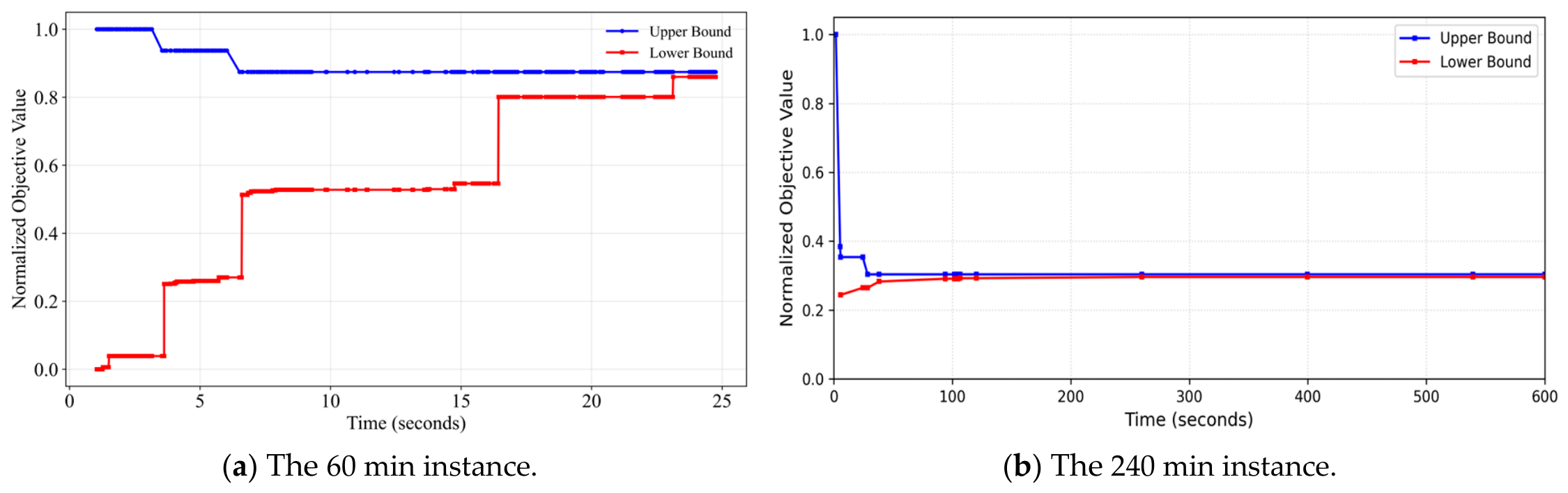
Figure 4 shows the normalized upper and lower bound convergence trajectories of Neur2BiLO-GBD for representative 60 min and 240 min instances. In the 60 min case, the bounds converge quickly and approach the optimum within a short time. In the 240 min case, the bounds tighten gradually as Benders cuts are added, indicating that the decomposition algorithm uses subproblem information to correct the master problem. For the 600 min instance, the GBD process must generate cuts iteratively, and the larger operating scale makes the master relaxation harder to approximate. The optimality gap therefore cannot fully close within the time limit. Nevertheless, Neur2BiLO-GBD stably obtains high-quality feasible solutions and provides valid optimality bounds under the given computational budget.

The computational tests characterize corridor-level scalability and robustness. Increasing the operating duration from 60 to 600 min expands the time–space network from 1464 to 14,424 nodes and simultaneously increases the coupling among aircraft circulation, charging, take-off/landing resources, and passenger-flow assignment. Accordingly, they show how solution performance changes with scheduling scale within the defined inter-hub feeder problem. The operating-scenario analyses complement these tests by varying fare, fleet size, charging resources, and external-transport delay, thereby examining how the conclusions change under different service-resource and passenger-response conditions in the corridor setting. Validation across multiple network topologies and demand patterns remains a topic for future work.

3.3. Scheduling Results

To illustrate baseline scheduling outcomes, this section examines flight execution, charging-pile occupation, passenger service, and representative aircraft trajectories.

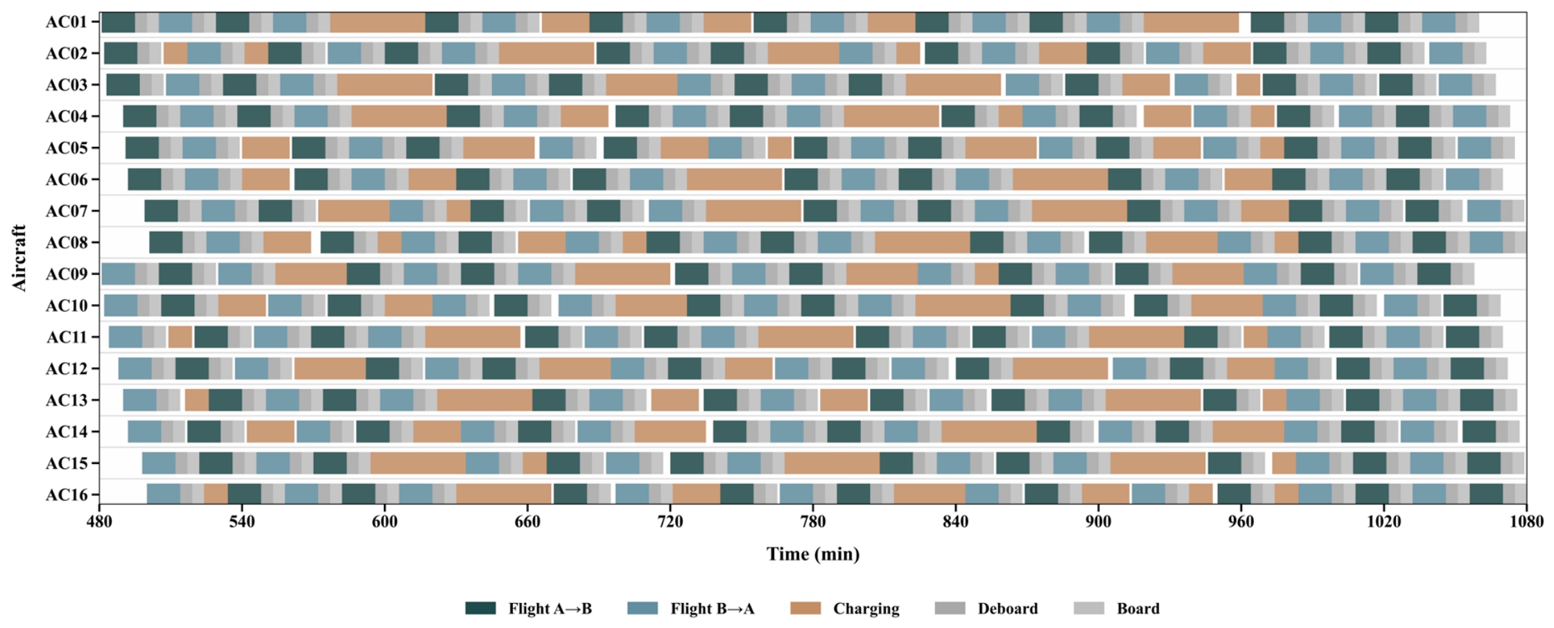
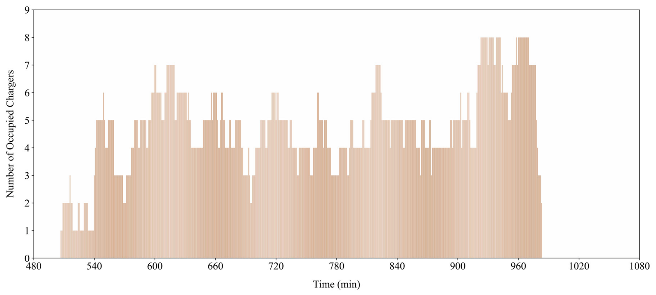
Figure 5 and Figure 6 show that the baseline timetable concentrates flight supply in the morning and evening demand peaks while preserving off-peak windows for charging and operational adjustment. No take-off or landing operation violates hub resource-capacity constraints, and charging-pile occupation remains within the system-wide capacity of the eight charging piles. The resulting schedule therefore maintains fleet circulation while satisfying the physical resource constraints.

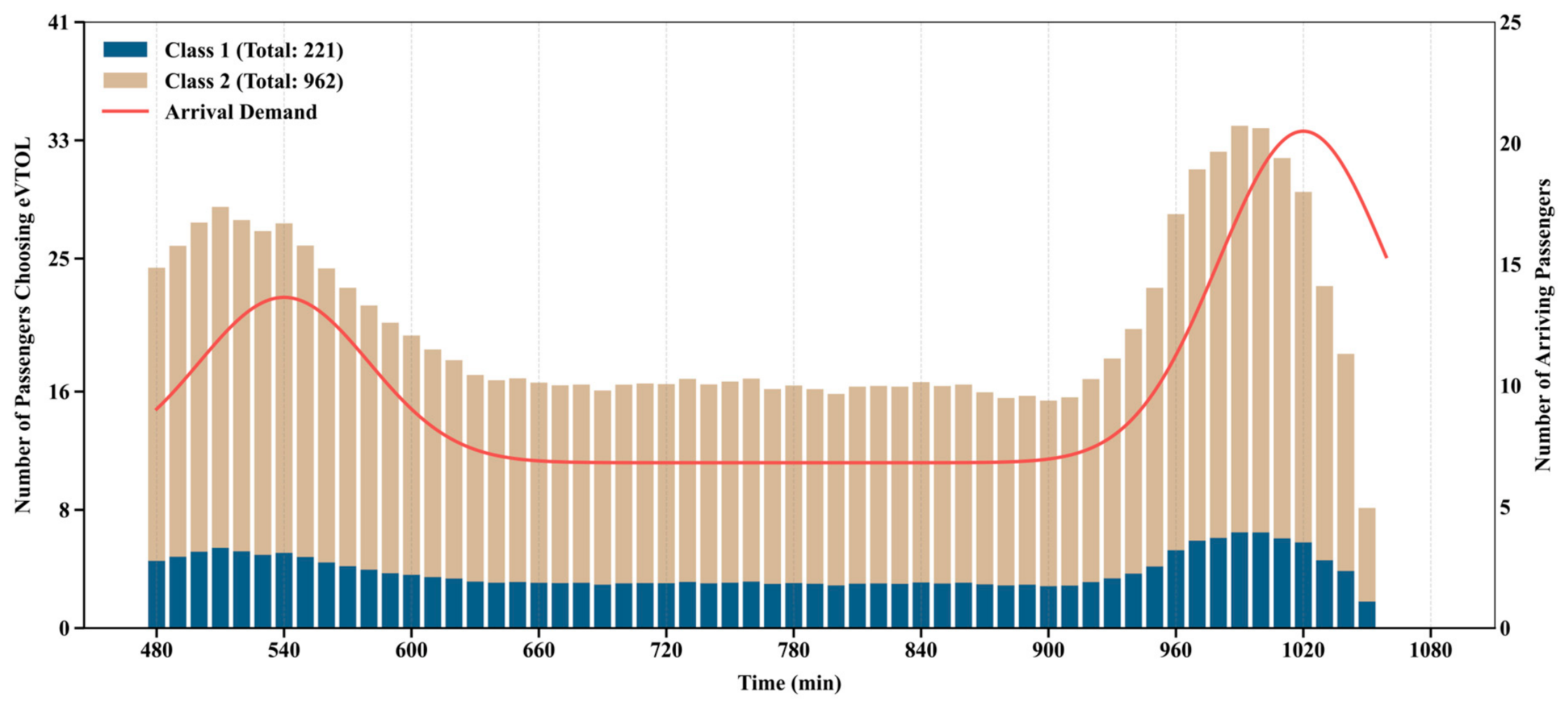
Passenger arrivals in Figure 7 exhibit a clear morning–evening double-peak pattern. eVTOL ridership rises with those peaks, but fleet size and seat capacity still leave a substantial share of demand to external transport. In total, 1183 passengers choose eVTOL, and Class 2 passengers account for the larger share of eVTOL ridership.

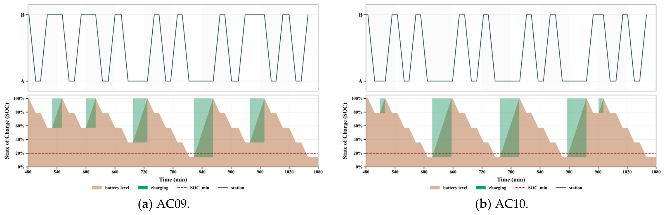
Figure 8 illustrates this coordination at the aircraft level. For AC09 and AC10, repeated flight tasks are sustained by multiple off-peak charging events, with SOC always remaining within the admissible range and without prolonged ineffective idle periods. These trajectories are consistent with a feasible timetable that coordinates demand peaks, charging, and fleet turnaround.

3.4. Resource-Configuration Effects

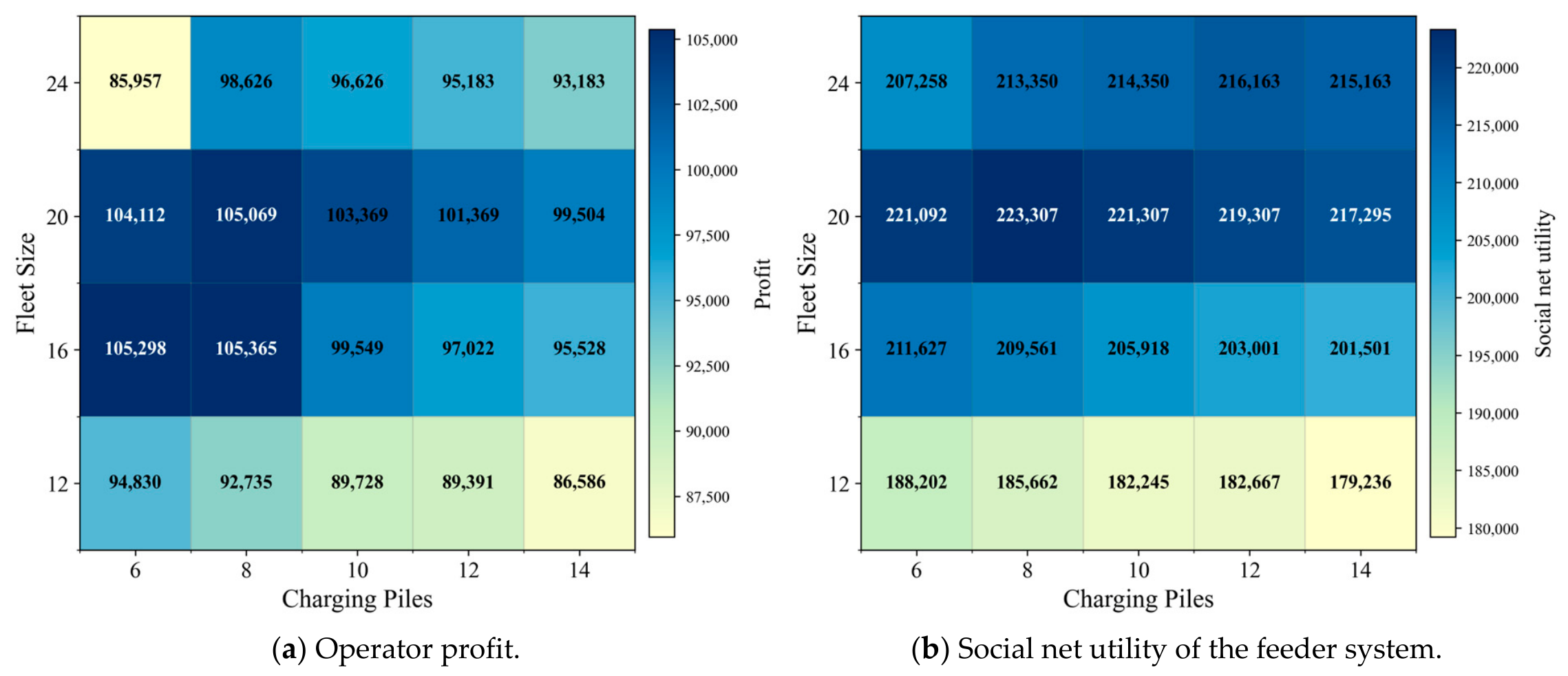
Under baseline fare, passenger demand, and external transport parameters, Figure 9 reveals a capacity-matching effect between fleet size and charging infrastructure. Operator profit increases as fleet size rises from 12 to 16 aircraft, but it declines when the fleet expands to 24 aircraft. For a fixed fleet size, adding charging piles is also beneficial only up to a point. With 16, 20, and 24 aircraft, profit rises when charging piles increase from 6 to 8, and then it falls as further charging investment raises fixed cost. When the fleet has only 12 aircraft, however, adding charging piles does not compensate for limited flight capacity. The main bottleneck is fleet size rather than charging availability.

The social net utility of the feeder system remains positive under all tested configurations, indicating that eVTOL entry yields net-positive benefits in the examined scenarios. Compared with operator profit, social net utility is more stable at larger fleet sizes. The 24-aircraft configuration yields lower profit than the 16–20-aircraft cases, yet it still maintains relatively high passenger-utility gains. Comparing the two heatmaps, the 20-aircraft, eight-pile configuration lies in a high-profit region and yields the highest social net utility in this experiment. Under the Hongqiao–Pudong setting, this combination best balances operating return and passenger-utility improvement. The 24-aircraft configuration still improves passenger utility, but higher fixed investment reduces social net utility.

3.5. Operational Scenario Analysis

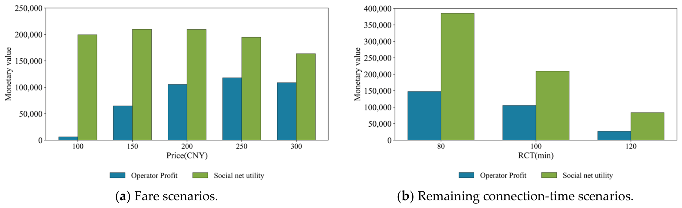
We analyze the effects of fare and remaining connection time under the baseline fleet and charging-facility configuration. Figure 10 shows that these two factors shape eVTOL feeder-service performance through different mechanisms. As fare increases, operator profit first rises and then falls, with a high-profit region near 250 CNY. Social net utility remains high, around 150–200 CNY, before declining. From a feeder-system perspective, fare changes reallocate eVTOL service value between operator revenue and passenger utility. Higher fares increase revenue per passenger but also raise generalized travel cost and weaken passenger-utility gains. The fare that maximizes profit therefore does not coincide with the fare that maximizes social net utility. The 100 CNY scenario does not yield the highest social net utility either, because excessively low fares weaken operator revenue and reduce overall system improvement. When the fare increases to 300 CNY, operator profit and social net utility both decline because demand contracts.

Remaining connection time affects how fully eVTOL’s time and reliability advantages translate into realized value. When RCT increases from 80 min to 120 min, both operator profit and social net utility decline markedly. Under tighter remaining connection time, passengers face stronger time pressure during inter-hub transfer, so eVTOL attracts more demand through its travel-time and reliability advantages. As remaining connection time relaxes, taxi/ride-hailing and airport express rail become more acceptable substitutes, reducing the marginal value of eVTOL. These results suggest that eVTOL feeder services are more attractive in high-urgency connection scenarios.

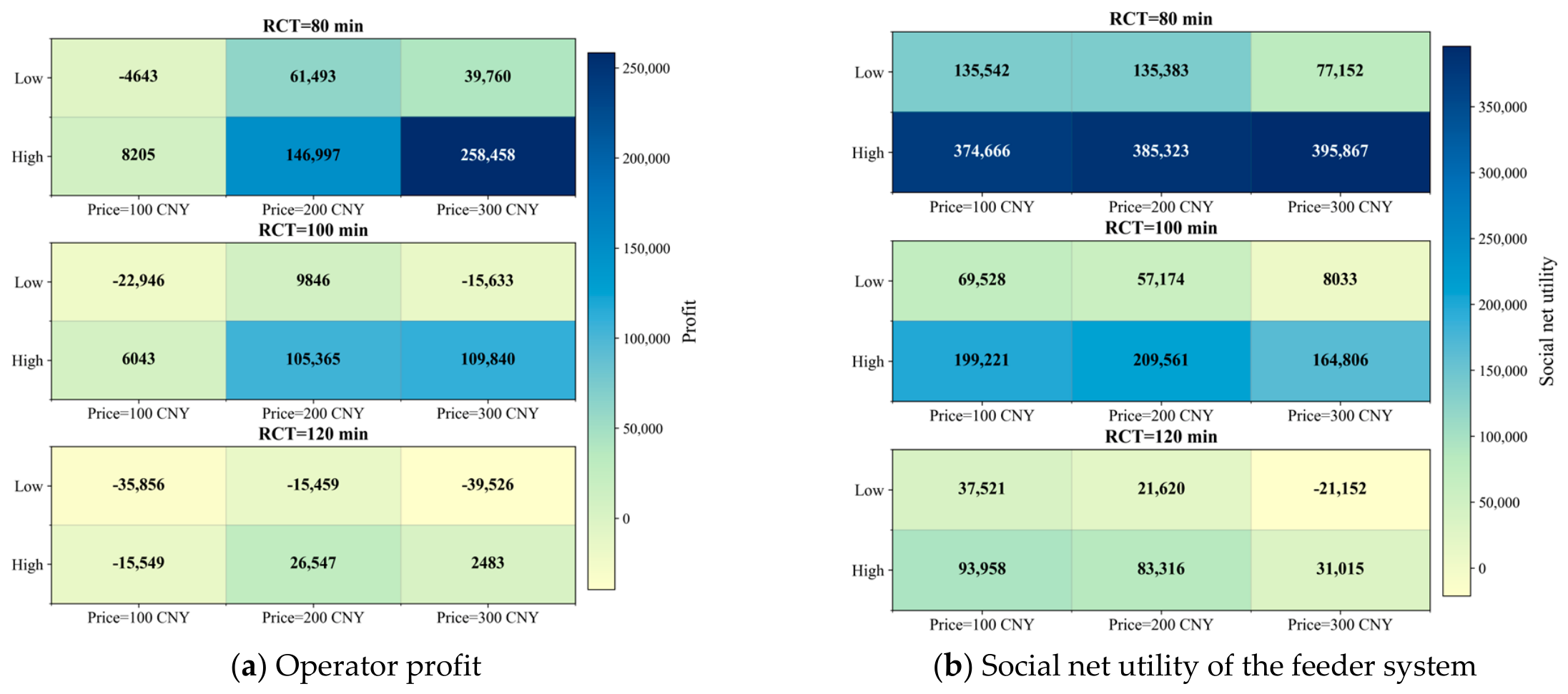
To examine how external transport reliability affects eVTOL feeder-service performance, this section varies remaining connection time, fare, and external-transport potential delay. As defined in Section 2.1, longer potential delay and shorter RCT strengthen delay-risk perception. The potential delay of eVTOL is fixed at 5 min. In the low-delay scenario, airport express rail and taxi delays are set to 5 min and 10 min, respectively. In the high-delay scenario, they are set to 10 min and 20 min. Other parameters remain unchanged.

As shown in Figure 11, higher external delay strengthens the value of reliable aerial feeder service, especially when RCT is short. Under low delay, higher-profit outcomes are concentrated near 200 CNY. Under higher external delay, the 200–300 CNY fare range maintains relatively high profit at RCT = 80 min and RCT = 100 min. Social net utility follows a different pattern. Under low delay, the high-value region is concentrated mainly in the 100–200 CNY range. Under high delay, even the 300 CNY scheme remains relatively high in social net utility at RCT = 80 min. At RCT = 100 min, relatively high social net utility is concentrated near 200 CNY. At RCT = 120 min, the 100 CNY scheme yields the highest social net utility. As remaining connection time relaxes, the high-value fare range shifts back toward lower fares.

This pattern arises because passengers place greater value on reliable feeder service when remaining connection time is short. Under such conditions, eVTOL’s time savings and reliability gains can sustain both higher fares and high social net utility. As remaining connection time relaxes, the marginal value of reliability improvement declines. Profit peaks therefore remain concentrated at medium-to-high fares, but the fare range associated with high social net utility shifts downward.

From a planning perspective, the results provide a screening rule for corridor deployment. Operators should prioritize corridors where short connection times and unreliable external transport create a sufficiently large reliability premium. Infrastructure planners can use the joint profit and social-net-utility surfaces to identify when additional aircraft or charging piles no longer produce proportional passenger benefits, while policymakers can evaluate whether pricing or infrastructure support is needed to keep the service viable under high-urgency conditions. These implications remain conditional on the planning-stage assumptions and should be reassessed when real-time disruption data and revealed-preference observations become available.

4. Conclusions

We develop a bilevel planning model for eVTOL feeder operations in transfer scenarios between integrated transport hubs and propose a Neur2BiLO-GBD hybrid solution framework to improve solution efficiency. The upper level selects eVTOL operation paths and schedules under specified fleet, charging-facility, and fare configurations, while the lower level captures heterogeneous passenger choices among feeder alternatives.

First, passenger choice of eVTOL feeder service shows clear heterogeneity. The parameter estimation results indicate that heterogeneity is mainly reflected in sensitivity to travel time and delay-risk perception, while differences in price sensitivity are relatively small. Numerical experiments further show that fare changes mainly affect total eVTOL demand, whereas transfer-time conditions and external transport reliability more strongly amplify differences in passenger response. Considering passenger heterogeneity is therefore important for evaluating eVTOL feeder services under time-sensitive inter-hub transfer conditions.

Second, the proposed Neur2BiLO-GBD framework improves the solution efficiency of the bilevel optimization model. In the 60 min case, the method obtains an objective identical to MKKT. In the 120 min case, it provides a feasible solution, whereas MKKT does not find a solution within the time limit. For the 240 min and larger cases, it delivers higher-quality feasible solutions and tighter optimality gaps than direct Neur2BiLO, while GA does not provide an optimality gap. Combining neural value-function approximation with Benders-type correction is therefore useful for large-scale eVTOL scheduling problems with nonlinear passenger-equilibrium responses.

Third, in the Hongqiao–Pudong inter-hub feeder case, eVTOL operational performance is strongly scenario-dependent. Increasing fleet size and charging facilities improves service capability, but marginal returns decline once supply exceeds demand. Fare level, remaining connection time, and external transport conditions jointly affect eVTOL market attractiveness. When passengers face tighter transfer-time constraints or lower reliability in external transport, eVTOL’s timeliness and reliability advantages are more likely to translate into higher operator profit and greater social net utility. In low-pressure transfer scenarios, external transport can satisfy most feeder demand, and eVTOL mainly plays a supplementary role. eVTOL therefore offers greater value in inter-hub scenarios with high time sensitivity and high reliability demand.

Fourth, operator profit and social net utility can differ substantially under different pricing schemes. The external-delay scenario analysis shows that, under high delay, regions of higher operator profit are concentrated in medium-to-high fare ranges, while the fare range with high social net utility shifts toward lower fares as remaining connection time becomes more relaxed. Operator profit mainly reflects the financial return from reliable feeder service, whereas social net utility also includes passenger-utility changes. When transfer time constraints are strong, medium-to-high fares can achieve both high operator profit and high social net utility. As remaining connection time relaxes, however, the high-social-utility fare range gradually falls below the high-profit fare range. eVTOL operating strategies should therefore consider both operator profit and social net utility, with fare and resource configurations selected according to the specific operating objective, such as prioritizing financial return, passenger-utility improvement, or a balance between the two. For operators, these results indicate that eVTOL feeder services are most attractive when passengers face short connection times and unreliable external transport. For infrastructure planners, fleet size and charging facilities should be expanded only until marginal improvements in service coverage and passenger utility begin to flatten. For policymakers, pricing and infrastructure support should account for both operator viability and passenger-time reliability.

This study has four main limitations. First, the numerical experiments are based on a single inter-hub feeder scenario and do not consider multi-origin-destination (OD) demand, node coordination, or route-network reconstruction in a multi-hub urban agglomeration network. Second, the model focuses on planning-stage scheduling and represents operational uncertainty in a simplified manner. Weather disturbances, airspace-capacity fluctuations, route conflicts, vehicle failures, service cancellations, and real-time passenger-arrival variations are not modeled as endogenous disruption-recovery processes. Third, passenger behavior parameters are mainly obtained from SP survey data and should be updated and calibrated using revealed-preference data once real operations become available. Fourth, from an algorithmic perspective, the current decomposition framework still has weak mixed-integer relaxation bounds in large-scale instances. Because 0–1 decisions and passenger-flow assignment are tightly coupled, the root-node relaxation remains loose and the optimality gap is difficult to close within the time limit. Future work can explore strengthened formulations based on path columns, aircraft-rotation columns, or time–space-arc flows, combined with column generation, branch-and-price, or logic-based Benders decomposition, to improve relaxation tightness and solution stability in large-scale eVTOL feeder networks.

References

1. Straubinger, A.; Rothfeld, R.; Shamiyeh, M.; Büchter, K.-D.; Kaiser, J.; Plötner, K.O. An overview of current research and developments in urban air mobility—Setting the scene for UAM introduction. J. Air Transp. Manag. 2020, 87, 101852. [Google Scholar] [CrossRef] [Scilit]
2. Cohen, A.P.; Shaheen, S.A.; Farrar, E.M. Urban Air Mobility: History, Ecosystem, Market Potential, and Challenges. IEEE Trans. Intell. Transp. Syst. 2021, 22, 6074–6087. [Google Scholar] [CrossRef] [Scilit]
3. Yan, Y.; Wang, K.; Qu, X. Urban air mobility (UAM) and ground transportation integration: A survey. Front. Eng. Manag. 2024, 11, 734–758. [Google Scholar] [CrossRef] [Scilit]
4. Zhang, H.G.; Liu, Z.Y.; Dong, Y.; Zhou, H.Y.; Liu, P.; Chen, J. A novel network equilibrium model integrating urban aerial mobility. Transp. Res. Part A Policy Pract. 2024, 187, 104160. [Google Scholar] [CrossRef] [Scilit]
5. Ren, Y.F.; Yang, M.; Chen, E.H.; Cheng, L.; Yuan, Y.L. Exploring passengers’ choice of transfer city in air-to-rail intermodal travel using an interpretable ensemble machine learning approach. Transportation 2024, 51, 1493–1523. [Google Scholar] [CrossRef] [Scilit]
6. Kleinbekman, I.C.; Mitici, M.A.; Wei, P. eVTOL arrival sequencing and scheduling for on-demand urban air mobility. In Proceedings of the 2018 IEEE/AIAA 37th Digital Avionics Systems Conference (DASC), London, UK, 23–27 September 2018; IEEE: Piscataway, NJ, USA, 2018; pp. 1–7. [Google Scholar] [CrossRef] [Scilit]
7. Pradeep, P.; Wei, P. Heuristic Approach for Arrival Sequencing and Scheduling for eVTOL Aircraft in On-Demand Urban Air Mobility. In Proceedings of the 2018 IEEE/AIAA 37th Digital Avionics Systems Conference (DASC), London, UK, 23–27 September 2018; IEEE: Piscataway, NJ, USA, 2018; pp. 1–7. [Google Scholar] [CrossRef] [Scilit]
8. Guo, Z.; Hao, M.; Liu, J.; Yu, B.; Jiang, Y. Joint routing and charging optimization for eVTOL aircraft recovery. Aerosp. Sci. Technol. 2022, 126, 107595. [Google Scholar] [CrossRef] [Scilit]
9. Wang, Y.; Li, J.; Yuan, Y.; Lai, C.S. Joint optimization of cost and scheduling for urban air mobility operation based on safety concerns and time-varying demand. Aerospace 2024, 11, 861. [Google Scholar] [CrossRef] [Scilit]
10. Yuan, Y.J.; Li, J.S.; Zhao, X.Y.; Wang, Y.T. eVTOL scheduling schemes for dynamic demand and variable intervals. Acta Aeronaut. Astronaut. Sin. 2026, 47, 631907. (In Chinese) [Google Scholar] [CrossRef]
11. Farazi, N.P.; Zou, B. Planning electric vertical takeoff and landing aircraft (eVTOL)-based package delivery with community noise impact considerations. Transp. Res. Part E Logist. Transp. Rev. 2024, 189, 103661. [Google Scholar] [CrossRef] [Scilit]
12. Jin, Z.; Ng, K.K.H.; Zhang, C.; Wang, M.; Yang, X. Integrated optimisation of strategic planning and service operations for urban air mobility systems. Transp. Res. Part A Policy Pract. 2024, 183, 104059. [Google Scholar] [CrossRef] [Scilit]
13. Zhang, J.; Guo, R.R.; Li, W.Q. Research on dynamic scheduling and route optimization strategy of flex-route transit considering travel choice preference of passenger. Systems 2024, 12, 138. [Google Scholar] [CrossRef] [Scilit]
14. Huang, D.; Hu, Z.T.; Tian, J.Y.; Tu, R. Improving conventional transit services with modular autonomous vehicles: A bi-level programming approach. Travel Behav. Soc. 2025, 39, 100939. [Google Scholar] [CrossRef] [Scilit]
15. Garrow, L.A.; German, B.J.; Leonard, C.E. Urban air mobility: A comprehensive review and comparative analysis with autonomous and electric ground transportation for informing future research. Transp. Res. Part C Emerg. Technol. 2021, 132, 103377. [Google Scholar] [CrossRef] [Scilit]
16. Boddupalli, S.S.; Garrow, L.A.; German, B.J.; Newman, J.P. Mode choice modeling for an electric vertical takeoff and landing (eVTOL) air taxi commuting service. Transp. Res. Part A Policy Pract. 2024, 181, 104000. [Google Scholar] [CrossRef] [Scilit]
17. Hwang, J.H.; Hong, S. A study on the factors influencing the adoption of urban air mobility and the future demand: Using the stated preference survey for three UAM operational scenarios in South Korea. J. Air Transp. Manag. 2023, 112, 102467. [Google Scholar] [CrossRef] [Scilit]
18. Zhou, Z.Y.; Cheng, L.; Yang, M.; Wang, L.C.; Chen, W.J.; Gong, J.; Zou, J. Analysis of passenger perception heterogeneity and differentiated service strategy for air-rail intermodal travel. Travel Behav. Soc. 2024, 37, 100872. [Google Scholar] [CrossRef] [Scilit]
19. Wang, B.Q.; Yang, M.; Feng, T.; Yang, Y.Y.; Yuan, Y.L. Heterogeneous choice of personalized Mobility-as-a-Service bundles and its impact on sustainable transportation. Transp. Res. Part D Transp. Environ. 2024, 131, 104224. [Google Scholar] [CrossRef] [Scilit]
20. Zhang, Z.; Lin, W.X.; Hu, T.Y.; Cao, Q.; Song, J.H.; Ren, G.; Wu, C.J. Passenger switch behavior and decision mechanisms in multimodal public transportation systems. Systems 2025, 13, 951. [Google Scholar] [CrossRef] [Scilit]
21. Jiang, Y.; Li, Z.; Wang, Y.; Xue, Q. Vertiport location for eVTOL considering multidimensional demand of urban air mobility: An application in Beijing. Transp. Res. Part A Policy Pract. 2025, 192, 104353. [Google Scholar] [CrossRef] [Scilit]
22. Guo, T.; Wu, H.; Lu, Q.-L.; Antoniou, C. Planning UAM network under uncertain travelers’ preferences: A sequential two-layer stochastic optimization approach. Transp. Res. Part A Policy Pract. 2025, 200, 104632. [Google Scholar] [CrossRef] [Scilit]
23. Wang, Y.C.; Yang, M.; Qin, B.Z.; Zhang, Y.Q. Decoding travel behavioral intentions under flight delays via interpretable machine learning: Insights for safeguarding passenger mobility. Transp. Res. Part A Policy Pract. 2025, 201, 104666. [Google Scholar] [CrossRef] [Scilit]
24. Ma, X.W.; Tian, X.L.; Cui, H.J.; He, M.J.; Wang, J.B.; Cheng, L. What influences intermodal choices: Metro-centric, bus-centric, hybrid? Insights from machine learning approaches. Transp. Res. Part D Transp. Environ. 2024, 136, 104407. [Google Scholar] [CrossRef] [Scilit]
25. Liu, Y.; Tang, R.; Shi, Z.B.; He, M.W.; Cheng, L. Shared mobility choices in metro connectivity: Shared bikes versus shared e-bikes. Transportation 2025, 52, 2187–2213. [Google Scholar] [CrossRef] [Scilit]
26. Fisk, C. Some developments in equilibrium traffic assignment. Transp. Res. Part B Methodol. 1980, 14, 243–255. [Google Scholar] [CrossRef] [Scilit]
27. Daganzo, C.F.; Sheffi, Y. On stochastic models of traffic assignment. Transp. Sci. 1977, 11, 253–274. [Google Scholar] [CrossRef] [Scilit]
28. Dixit, M.; Cats, O.; Brands, T.; van Oort, N.; Hoogendoorn, S. Perception of overlap in multi-modal urban transit route choice. Transp. A Transp. Sci. 2023, 19, 2005180. [Google Scholar] [CrossRef] [Scilit]
29. Tan, H.; Du, M.; Chen, A. Accelerating the gradient projection algorithm for solving the non-additive traffic equilibrium problem with the Barzilai-Borwein step size. Comput. Oper. Res. 2022, 141, 105723. [Google Scholar] [CrossRef] [Scilit]
30. Nair, V.; Bartunov, S.; Gimeno, F.; von Glehn, I.; Lichocki, P.; Lobov, I.; O’Donoghue, B.; Sonnerat, N.; Tjandraatmadja, C.; Wang, P.; et al. Solving mixed integer programs using neural networks. arXiv 2020, arXiv:2012.13349. [Google Scholar] [CrossRef] [Scilit]
31. Dumouchelle, J.; Julien, E.; Kurtz, J.; Khalil, E. Neur2BiLO: Neural Bilevel Optimization. In Proceedings of the Advances in Neural Information Processing Systems 37; Neural Information Processing Systems Foundation, Inc.: San Diego, CA, USA, 2024; pp. 86688–86719. [Google Scholar] [CrossRef] [Scilit]
32. Fischetti, M.; Jo, J. Deep neural networks and mixed integer linear optimization. Constraints 2018, 23, 296–309. [Google Scholar] [CrossRef] [Scilit]
33. Benders, J.F. Partitioning procedures for solving mixed-variables programming problems. Numer. Math. 1962, 4, 238–252. [Google Scholar] [CrossRef] [Scilit]
34. Geoffrion, A.M. Generalized Benders decomposition. J. Optim. Theory Appl. 1972, 10, 237–260. [Google Scholar] [CrossRef] [Scilit]
35. Borozan, S.; Giannelos, S.; Falugi, P.; Moreira, A.; Strbac, G. Machine learning-enhanced Benders decomposition approach for the multi-stage stochastic transmission expansion planning problem. Electr. Power Syst. Res. 2024, 237, 110985. [Google Scholar] [CrossRef] [Scilit]
36. Train, K.E. Discrete Choice Methods with Simulation, 2nd ed.; Cambridge University Press: Cambridge, UK, 2009. [Google Scholar] [CrossRef] [Scilit]
37. Rose, J.M.; Bliemer, M.C.J. Constructing efficient stated choice experimental designs. Transp. Rev. 2009, 29, 587–617. [Google Scholar] [CrossRef] [Scilit]
38. Xu, H.; Lou, Y.; Yin, Y.; Zhou, J. A prospect-based user equilibrium model with endogenous reference points and its application in congestion pricing. Transp. Res. Part B Methodol. 2011, 45, 311–328. [Google Scholar] [CrossRef] [Scilit]
39. McFadden, D. Conditional logit analysis of qualitative choice behavior. In Frontiers in Econometrics; Zarembka, P., Ed.; Academic Press: New York, NY, USA, 1974; pp. 105–142. [Google Scholar]
40. Fraley, C.; Raftery, A.E. Model-based clustering, discriminant analysis, and density estimation. J. Am. Stat. Assoc. 2002, 97, 611–631. [Google Scholar] [CrossRef] [Scilit]
41. Rousseeuw, P.J. Silhouettes: A graphical aid to the interpretation and validation of cluster analysis. J. Comput. Appl. Math. 1987, 20, 53–65. [Google Scholar] [CrossRef] [Scilit]
42. Chiou, S.W. Bilevel programming for the continuous transport network design problem. Transp. Res. Part B Methodol. 2005, 39, 361–383. [Google Scholar] [CrossRef] [Scilit]
43. Sheffi, Y. Urban Transportation Networks: Equilibrium Analysis with Mathematical Programming Methods; Prentice-Hall: Englewood Cliffs, NJ, USA, 1985. [Google Scholar]
44. Chen, J. Integrated routing and charging scheduling for autonomous electric aerial vehicle system. In Proceedings of the 2019 IEEE/AIAA 38th Digital Avionics Systems Conference (DASC), San Diego, CA, USA, 8–12 September 2019; IEEE: Piscataway, NJ, USA, 2019; pp. 1–7. [Google Scholar] [CrossRef] [Scilit]
45. Geister, D.; Korn, B. Density based Management Concept for Urban Air Traffic. In Proceedings of the 2018 IEEE/AIAA 37th Digital Avionics Systems Conference (DASC), London, UK, 23–27 September 2018; IEEE: Piscataway, NJ, USA, 2018; pp. 1–9. [Google Scholar] [CrossRef] [Scilit]
46. Zhong, G.; Wan, X.; Zhang, J.; Yin, T.; Ran, B. Characterizing passenger flow for a transportation hub based on mobile phone data. IEEE Trans. Intell. Transp. Syst. 2017, 18, 1507–1518. [Google Scholar] [CrossRef] [Scilit]
47. Federal Aviation Administration. Advanced Air Mobility (AAM) Implementation Plan: Near-Term (Innovate28) Focus with an Eye on the Future of AAM, Version 1.0; FAA: Washington, DC, USA, 2023. Available online: https://www.faa.gov/sites/faa.gov/files/AAM-I28-Implementation-Plan.pdf (accessed on 9 June 2026).
48. Jiang, F.; Wang, L.; Huang, S. Analysis of the transfer time and influencing factors of air-rail integration passengers: A case study of Shijiazhuang Zhengding International Airport. Sustainability 2022, 14, 16193. [Google Scholar] [CrossRef] [Scilit]
49. Chen, L.; Yao, E.; Yang, Y.; Pan, L.; Liu, S. Understanding passengers’ intermodal travel behavior to improve air-rail service: A case study of Beijing-Tianjin-Hebei urban agglomeration. J. Air Transp. Manag. 2024, 118, 102615. [Google Scholar] [CrossRef] [Scilit]
50. Ke, Y.; Nie, L.; Yuan, W. Joint optimization of flight and train timetables for air and high-speed railway integration services with maximum accessibility. Transp. B Transp. Dyn. 2022, 10, 207–236. [Google Scholar] [CrossRef] [Scilit]
Figure 1. Model hyperparameter calibration and optimal class-number evaluation. (a) Curvature parameter calibration. (b) Bayesian information criterion (BIC) evaluation. (c) Silhouette evaluation. The red dots in panels (a) and (b) indicate the selected values of κ = 12 and   G = 2 , respectively.
Systems 14 01109 g001
Figure 2. Time–space network schematic.
Systems 14 01109 g002
Figure 3. Inter-hub feeder scenario between Hongqiao Hub and Pudong International Airport.
Systems 14 01109 g003
Figure 4. Convergence trajectories of Neur2BiLO-GBD.
Systems 14 01109 g004
Figure 5. Baseline eVTOL fleet operation Gantt chart.
Systems 14 01109 g005
Figure 6. Charging-facility occupation under the baseline scenario.
Systems 14 01109 g006
Figure 7. Passenger arrival demand and eVTOL ridership.
Systems 14 01109 g007
Figure 8. Representative eVTOL operation trajectories and charging processes.
Systems 14 01109 g008
Figure 9. eVTOL feeder-service performance under different resource configurations.
Systems 14 01109 g009
Figure 10. eVTOL feeder-service performance under different fare and remaining connection-time scenarios.
Systems 14 01109 g010
Figure 11. eVTOL feeder-service performance under external-delay scenarios.
Systems 14 01109 g011