Article

Performance Pursuit Behavior of Autonomous Vehicles: An Area-Based Driving Strategy for Autonomous Vehicles Considering Multi-Objective Optimization at Signalized Intersections

1
School of Energy and Power Engineering, North University of China, Taiyuan 030051, China
2
College of Engineering, Ocean University of China, Qingdao 266100, China
3
College of Engineering, Zhejiang Normal University, Jinhua 321004, China
*
Author to whom correspondence should be addressed.
Systems 2026, 14(7), 852; https://doi.org/10.3390/systems14070852
Submission received: 16 April 2026 / Revised: 14 July 2026 / Accepted: 14 July 2026 / Published: 17 July 2026
(This article belongs to the Section Artificial Intelligence and Digital Systems Engineering)

Abstract

Autonomous driving technology enables precise motion control and creates substantial opportunities for improving the operation of signalized intersections. However, the performance trade-offs among autonomous vehicles at signalized intersections, and their impacts on the operation process, will directly affect the further application of autonomous driving in the intelligent transportation system. Addressing this research focus, this paper proposes a multi-objective driving strategy for autonomous vehicles based on the scene characteristics of signalized intersections. Firstly, the intersection and its adjacent control area are treated as an integrated decision region, and an autonomous vehicle driving performance model at signalized intersections is established to evaluate economy, comfort, and efficiency performance. Secondly, a multi-stage trajectory generation method combining phase division, candidate trajectory generation, and real-time trajectory adjustment is further developed to adapt the ego vehicle to traffic conditions while maintaining safe and smooth motion. Thirdly, a multi-objective optimization problem is formulated to generate optimal trajectories for each autonomous vehicle within the region. Finally, weight sensitivity analysis, application adaptability analysis, and an analysis of system-level key factors and system-level impacts are conducted to explore the strategy optimization potential. The case studies reveal that the proposed strategy achieves improvements of 50.0%, 33.3%, and 21.6% in comfort, economy, and efficiency, respectively, compared with the common strategy. In future research, more specific and complex practical factors will be incorporated into the proposed strategy. The strategy helps to reveal the performance-oriented behavior of autonomous vehicles at signalized intersections and provides methodological support for the wider application of autonomous driving in intelligent transportation systems.

1. Introduction

Signalized intersections are critical nodes in urban road networks and strongly affect the performance of the entire intelligent transportation system [1]. However, the complex interactions among vehicles, pedestrians, and signal control make these locations especially vulnerable to safety and operational problems. Empirical studies have shown that urban signalized intersections remain crash-prone locations and that signal-related characteristics can substantially affect crash frequencies [2]. Meanwhile, signalized intersections are also recognized as hot spots for fuel consumption and emissions because repeated stopping, idling, deceleration, and acceleration increase both travel delays and energy use [3]. Nevertheless, the conventional intersection-passing mode dominated by human drivers is constrained by the heterogeneity of driver responses, the locality of decision-making, and the discreteness of vehicle control, which often leads to persistent trade-offs among safety, efficiency, and economy. Therefore, when vehicles travel through signalized intersections, it is necessary to abandon the one-sided pursuit of a single performance indicator and implement the multi-objective collaborative optimization of vehicle driving performance according to the actual traffic operating conditions. While complying with traffic rule constraints and guaranteeing fundamental driving safety, the dynamic balance and overall optimality of multiple driving performance aspects can be realized, which further improves the comprehensive traffic efficiency of urban road intersections.
The rapid development of autonomous driving technology provides a new way to address long-standing operational problems at urban signalized intersections [4,5]. Autonomous vehicles feature precise motion control, predictable trajectories, and efficient environmental perception, and they can further exploit V2X communication to coordinate individual and group behavior. An intelligent transportation system is a new-generation transportation system centered on the coordination of vehicles, roads, and clouds. The in-depth integration of the vehicle side, road side, and cloud side jointly constructs an efficient, safe, economical, and comfortable smart transportation operation environment. Relying on the vehicle–road–cloud collaborative architecture, autonomous driving technology realizes multi-dimensional improvements in traffic efficiency, driving safety, and traffic management modes, which comprehensively promote the intelligent, collaborative, and refined development of intelligent transportation systems. With the support of vehicle–infrastructure cooperation, autonomous vehicles can obtain real-time information on signal timing, road conditions, and surrounding traffic states, which transforms signalized intersections from conflict points into intelligently managed and coordinately controlled zones. This transformation not only reduces efficiency losses and safety risks caused by human-driving heterogeneity but also creates conditions for achieving global optimization under the coupled objectives of safety, efficiency, energy consumption, and ride comfort. Therefore, area-based driving strategies for autonomous vehicles at signalized intersections have become an important research direction, with strong theoretical and practical value in intelligent transportation systems. It is worth noting that the problem discussed in this paper is not limited to the driving states of individual vehicles. The local decision-making of autonomous vehicles affects their energy consumption, riding comfort, and travel time. The superposition and accumulation of such local changes can further influence traffic flow stability and the operational states of signalized intersections, as well as the vehicle–road–cloud collaborative intelligent transportation system. Therefore, the core research focus of this paper lies in two aspects: the multi-objective optimization of economy, comfort, and traffic efficiency through feasible driving trajectory planning for autonomous vehicles within the control areas of signalized intersections and the influence mechanisms of vehicle-side, road-side, and cloud-side factors on the local performance-oriented driving behavior of autonomous vehicles.

1.1. Autonomous Driving Strategies

Autonomous driving strategies refer to the driving decisions independently formulated and implemented by autonomous vehicles based on environmental perception, road condition information, traffic rules, and vehicle self-states, combined with preset logical rules and optimization objectives [6,7,8,9,10,11,12,13,14,15,16,17]. Autonomous driving strategies generally rely on the closed-loop coordination of environment perception, behavioral decision-making, trajectory planning, and tracking control. Existing studies have therefore focused on how to achieve a balanced improvement in safety, efficiency, energy consumption, and ride comfort in complex and dynamic traffic environments, and the representative research can be grouped into the four technical modules reviewed below.
The perception and prediction module serves as the frontend and fundamental component of the autonomous driving system, undertaking the core functions of environmental cognition and future traffic state prediction. Recent studies have mainly aimed to overcome sensor limitations and improve the robustness of scene understanding and motion inference. Florea et al. [6] enhanced the accuracy of single-sensor perception through semantic and geometric data fusion; Geng et al. [7] proposed a dynamic learning spatial–temporal Transformer network for vehicle trajectory prediction at urban intersections; and Wu et al. [8] developed the CrossFuser multimodal fusion framework, which improves the reliability of perception under complex and previously unseen conditions. The perception and prediction module provides a fundamental input basis for subsequent behavioral decision-making. Reliable behavioral decision-making serves as the core prerequisite for autonomous vehicles to safely navigate urban road scenarios. In behavioral decision-making, the main challenge is to address uncertainty and multi-agent interaction in urban traffic. Bouton et al. [9] formulated autonomous intersection driving as a partially observable Markov decision process and combined it with Monte Carlo tree search to improve safety and efficiency. Yoon et al. [10] integrated spline-based RRT* with Bézier curves to achieve efficient collision-free planning for car-like vehicles, while Feng et al. [11] proposed a hierarchical architecture with the entry vehicle location and speed method to coordinate traffic flow segmentation and signal timing scheduling. On the basis of reasonable behavioral decision-making, high-quality trajectory planning and optimization are crucial for converting decision instructions into feasible vehicle motion states. In trajectory planning and optimization, the core objective is to generate smooth, feasible, and constraint-satisfying motions. Werling et al. [12] proposed a semi-reactive planning strategy for long-term maneuvers such as lane changing and car following; Qian et al. [13] developed the synchronized maneuver search and trajectory planning algorithm to couple maneuver selection with trajectory generation in dynamic environments; and Jin et al. [14] adopted a quintic-polynomial approach to construct trajectories that maintain smooth and continuous state evolution under different driving conditions. After trajectory planning, high-precision trajectory tracking and motion control are further required to resist external disturbances and guarantee driving stability. At the tracking–control level, existing studies have focused on maintaining accurate trajectory execution in the presence of model uncertainty and external disturbances. Vaskov et al. [15] proposed a friction-adaptive stochastic nonlinear model predictive controller for uncertain road conditions; Feng et al. [16] established an adaptive terminal sliding-mode tracking strategy for autonomous vehicles with unknown parameters and disturbances; and Zeng et al. [17] introduced a deep Bayesian inverse reinforcement learning framework that achieves more human-like driving behavior than conventional inverse reinforcement learning methods. The literature has established a relatively complete technical chain from perception and prediction to decision-making, trajectory generation, and control execution. However, most studies still emphasize a single module or a limited set of objectives, and fewer works explicitly address region-level coordination among safety, efficiency, energy consumption, and ride comfort at signalized intersections.

1.2. Signalized Intersection Optimization Strategies

Signalized intersection optimization has been widely studied to mitigate congestion, excessive delays, and energy waste caused by repeated stopping and starting under conventional signal control. With the support of vehicle-to-infrastructure communication, existing studies have mainly focused on two closely related directions: speed guidance optimization for individual or connected vehicles and signal timing optimization for coordinated traffic operations.
The objective of speed guidance optimization is usually to exploit real-time signal phase and traffic-state information to generate non-stop, collision-free, or energy-efficient speed profiles. Xu et al. [18] showed that the cooperative optimization of signal timing and vehicle speeds in an automated driving environment can significantly reduce stops and travel times. Yang et al. [19] optimized upstream and downstream speed profiles while accounting for signal information and queue conditions, thereby reducing fuel consumption. Ubiergo and Jin [20] further proposed an eco-driving strategy based on advisory speed limits for connected vehicles, following their predecessors, rather than direct speed control. In addition to speed guidance optimization, signal timing optimization serves as another core means to improve the operational efficiency of signalized intersections. In signal timing optimization, the emphasis has been on overcoming the limitations of isolated intersection control through adaptive, agent-based, or coordinated strategies. Abdulhai et al. [21] treated traffic lights at successive intersections as multiple agents and applied Q-learning to optimize timing under varying traffic demands. Zhao et al. [22] proposed a variable-cycle green-wave bandwidth coordination method integrated with traffic-responsive control, and Xu et al. [23] established a hierarchical collaborative optimization framework for traffic signals and connected and automated vehicles (CAVs), thereby improving system-level performance at signalized intersections. Existing studies on signalized intersections have formed a relatively mature technical framework centered on speed guidance and signal timing, and these efforts have delivered clear gains in traffic efficiency and energy savings. Nevertheless, most of the available methods still focus on isolated vehicles, isolated intersections, or isolated objectives, which leaves room for a region-based multi-objective driving strategy that explicitly coordinates vehicle motion with the surrounding traffic environment.
In summary, research on autonomous driving and signalized intersection optimization has established mature technical systems. However, existing studies still present evident deficiencies. Many autonomous driving studies only achieve local optimization of individual module performance or single indicators, including safety, efficiency, and energy consumption, and lack regional multi-objective collaborative optimization oriented toward complex and dynamic signalized intersection scenarios. Meanwhile, current intersection optimization methods are mostly limited to single-vehicle optimization and fail to realize the in-depth coupling between vehicle motion control and regional traffic environments, making it difficult to fully improve the overall traffic performance of intersections. Focusing on the typical performance trade-off of signalized intersections, this paper proposes an area-based driving strategy for autonomous vehicles considering economic, comfort, and efficiency under the guarantee of safety. The core of the strategy lies in abandoning the traditional independent decision-making model for single vehicles and defining the intersection and its adjacent areas as an integrated control unit. By integrating real-time status information about all relevant vehicles and the signal timing sequence of the intersection, a multi-objective optimization problem is formulated with the core objectives of reducing traffic delays, total energy consumption, and discomfort under the guarantee of safety. Optimization is adopted to generate smooth and safe optimal trajectories for each autonomous vehicle within the region. This study aims to fundamentally reconcile the multi-objective trade-off at signalized intersections through the proposed regional cooperative driving strategy, verify the great potential of autonomous driving technology in improving the comprehensive operational performance of intersections, and provide theoretical and methodological support for key control technologies in the next-generation intelligent transportation system. To concentrate on the behavioral characteristics reflecting the performance pursuit of autonomous vehicles at signalized intersections, this study simplifies practical factors in the model and simulation environment, such as algorithm execution delays and pedestrian interference.
To fill the above gaps, this paper proposes an area-based driving strategy for autonomous vehicles considering economic, comfort, and efficiency under the guarantee of safety. The research contributions of this paper are reflected in the regionalized organization of the trajectory generation process; the establishment of performance models targeting economy, comfort, and energy efficiency; and the adoption of scenario-based tests. The proposed strategy is validated to clarify its adaptability to variations in key factors, including the traffic demand, signal timing, trigger region length, autonomous vehicle penetration rate, benchmark strategies, and perception disturbances. The remainder of the paper is organized as follows: Section 2 analyzes the operation of signalized intersections in intelligent transportation systems. Section 3 introduces the autonomous vehicle driving performance model at signalized intersections. Section 4 explains an area-based trajectory generation model considering multi-stage risk avoidance. Section 5 introduces an area-based multi-objective driving strategy for autonomous vehicles. Case studies and discussions related to sensitivity and adaptability are presented in Section 6. Section 7 concludes the paper and provides insights for future research.

2. Operation Analysis of Signalized Intersections in Intelligent Transportation Systems

As the core hubs of the transportation system, signal-controlled intersections are critical nodes with a high incidence of traffic conflicts, congestion, and traffic accidents. Their operational status directly determines the traffic efficiency, driving safety level, and energy consumption of the regional road network [1,4,6]. With the rapid development of technologies such as autonomous driving, information exchange, and artificial intelligence, the transportation system will evolve into an intelligent transportation system composed of a vehicle road cloud. Focusing on the driving process of autonomous vehicles, this section elaborates on the system composition and interactive mechanisms of signalized intersections in intelligent transportation systems, as well as the optimization potential of autonomous driving technologies. It is worth noting that, in the model established in this paper, this architecture only serves as the information support basis for trajectory planning. Specifically, the vehicle end provides self-vehicle state information, the road end supplies traffic signal and local traffic data, and the cloud end outputs the time domain of regional planning. This study does not construct complete cloud computing algorithms or communication protocols; instead, it adopts this architecture to define the information boundary and control scope for the subsequent performance model.

2.1. System Composition

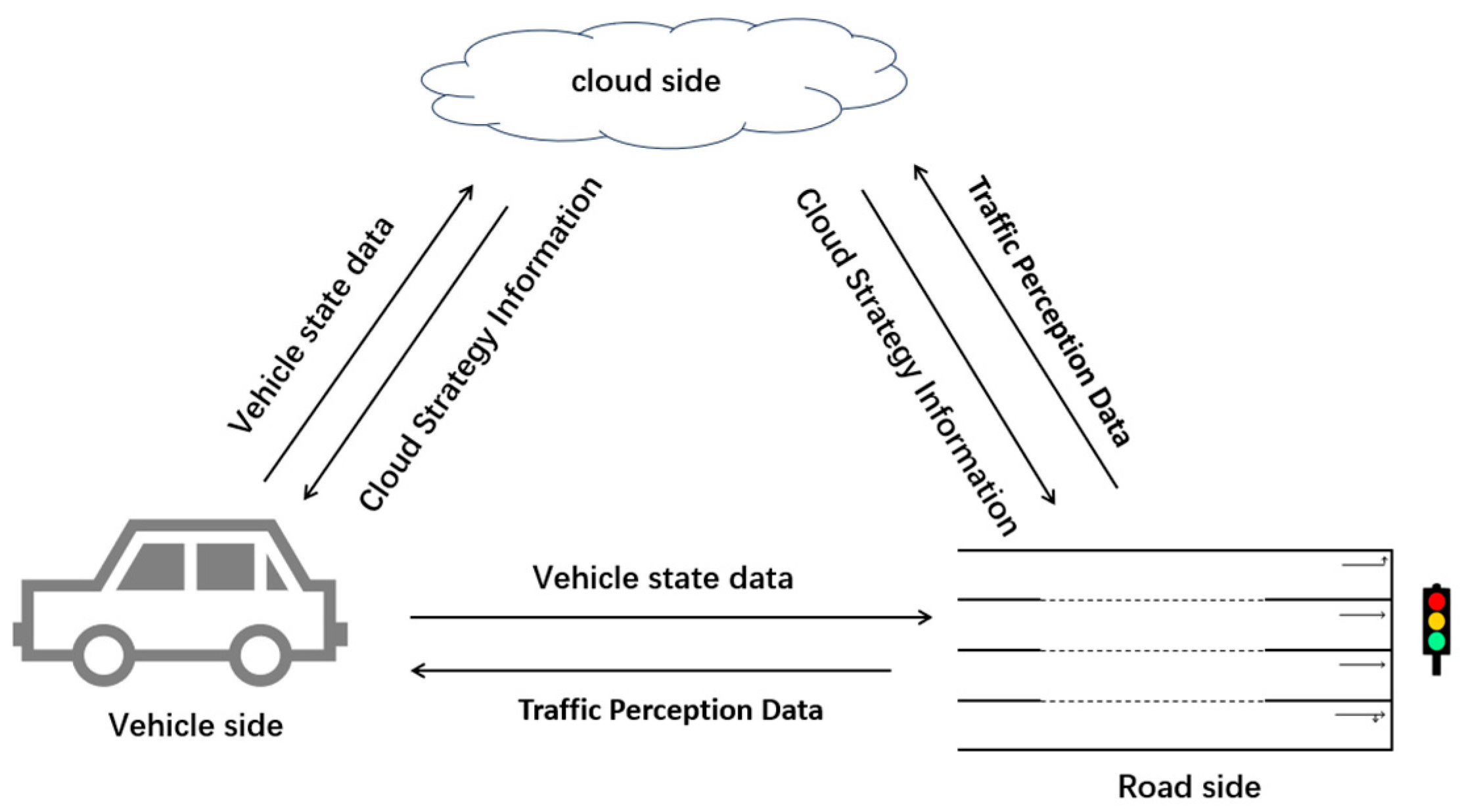
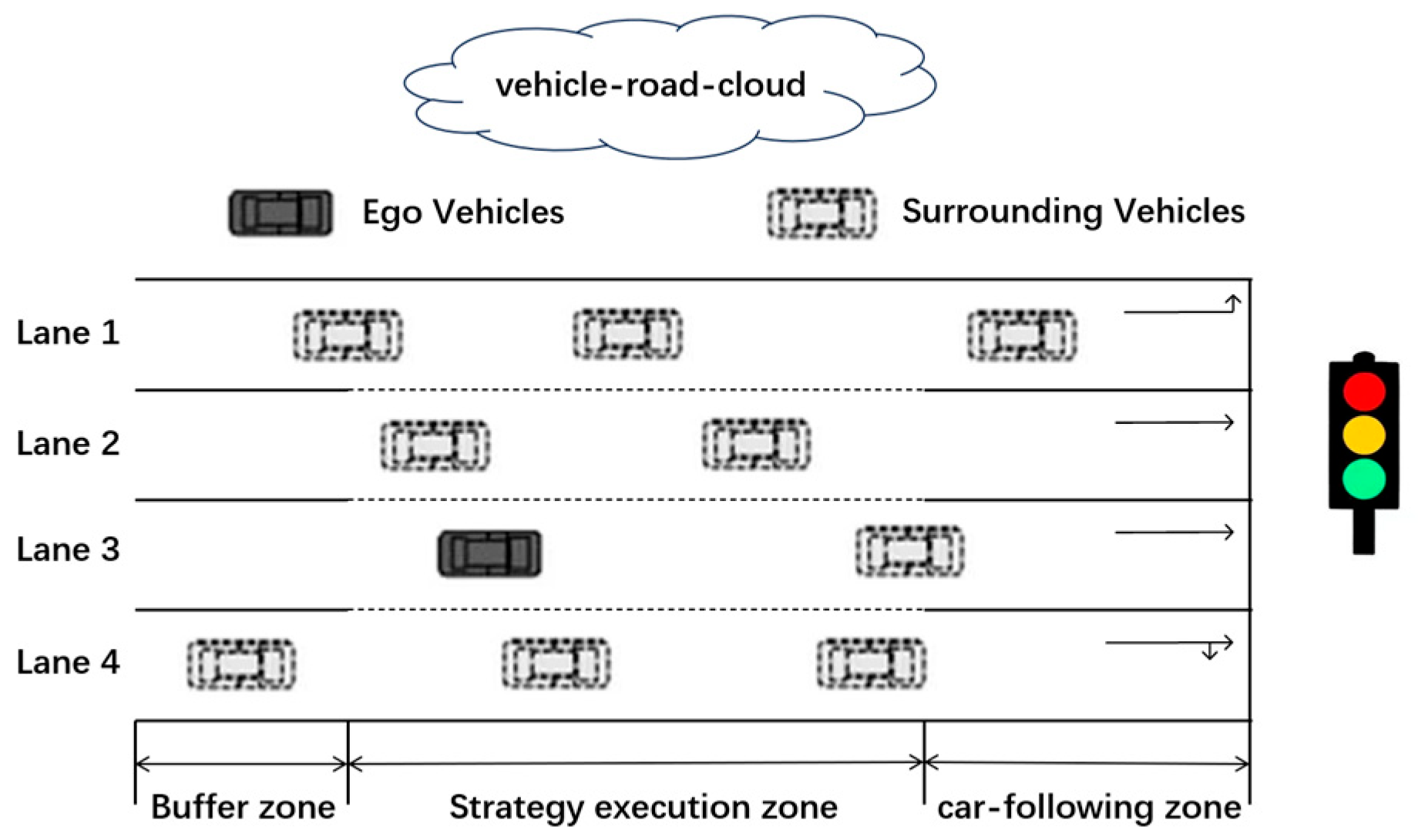
Intelligent signalized intersections serve as the core control nodes of regional road networks; they are mainly applied to direct and connect traffic flows and act as crucial carriers for dynamic management and control in the intelligent transportation system [9,18]. During the operation of autonomous vehicles at intelligent intersections, the vehicle–road–cloud integrated system adopted is collaboratively composed of three modules: vehicles, the roadside, and the cloud. The schematic diagram can be seen in Figure 1.
With intelligent connected vehicles as the carriers, they realize environmental perception, decision-making, and motion control through onboard units, multi-modal sensors, and autonomous driving systems, and they upload vehicle status and driving intention data in real time. The roadside system consists of roadside units, LiDAR, high-definition cameras, and edge computing nodes deployed at intersections. It completes the full-scale perception of traffic participants, signal light states, and the traffic operation status at intersections, as well as data preprocessing and collaborative decision-making, and it transfers environmental perception data and traffic passage instructions to connected vehicles. As the core hub of the entire system, the cloud platform integrates dynamic road network data, high-precision maps, and massive traffic big data. It conducts global traffic situation analysis, the coordinated scheduling of group vehicles, and signal timing optimization and provides autonomous vehicles with global path planning, early safety warnings, and optimal driving strategies, so as to ensure that autonomous vehicles pass through intelligent signalized intersections in a safe and efficient manner.

2.2. Interaction Mechanism

The vehicle–road–cloud interaction serves as the core support for the efficient operation of intelligent signalized intersections [6,8]. It refers to the dynamic information exchange and collaborative cooperation among vehicles, roadside facilities, and cloud platforms. Vehicles act as the main body of information collection and execution; roadside facilities undertake information transmission and omnidirectional perception; and the cloud platform functions as the core for information analysis and decision-making. The three participants operate and interact following a clear logical mechanism. When autonomous vehicles travel through intelligent intersections, they collect driving status data in real time and transmit such information to roadside facilities and the cloud platform. Roadside devices perceive environmental information within the intersection and synchronously deliver decision instructions issued by the cloud platform to vehicles. The cloud platform aggregates multi-source data, formulates optimized strategies combined with the operational state of the regional road network, and distributes the formulated strategies to roadside facilities and vehicles.
Vehicle–road–cloud interaction realizes real-time communication between vehicles and intersection environments, provides comprehensive environmental perception for autonomous vehicles, and ensures the timely update and accurate execution of control strategies [4,6]. Meanwhile, it breaks the limitations of isolated single-point management, improves the collaborative optimization capabilities of the regional road network, and provides a fundamental guarantee for the stable operation of intelligent signalized intersections. Ultimately, it contributes to the realization of safe, economical, comfortable, and high-efficiency traffic control at intersections.

2.3. Optimization Potential of Autonomous Driving Technology

Autonomous vehicles’ core support lies in the onboard perception module, decision-making module, control module, and communication module [4,8]. The onboard perception module collects environmental information around the vehicle, the decision and control module formulates driving strategies, and the communication module realizes information interaction with the vehicle–road–cloud system.
As an important part of the intelligent transportation system, autonomous vehicles have the potential to achieve safety, economy, comfort, and efficiency in the driving process, due to their precise control of movement [11,13]. Moreover, the performance of individual vehicles will affect the operational state of the entire transportation system through the clustering effect. In the environment of the intelligent signalized intersection, autonomous vehicles possess remarkable optimization potential in terms of driving safety, traffic efficiency, driving comfort, energy consumption, and emissions by virtue of their superior perception, decision-making, execution, and vehicle–road–cloud collaboration capabilities. Combined with the collaborative control of intelligent roadside facilities and cloud platforms, autonomous driving can break through the efficiency bottleneck of traditional traffic systems and realize improvements in operational efficiency at intersections and even across the entire road network.
This vehicle-level optimization also has broader implications. When many autonomous vehicles adopt similar performance pursuit behavior, local changes in speed smoothness, lane selection, and signal response may accumulate into changes in intersection efficiency, regional energy use, and the operational stability of the intelligent transportation system. This is the main reason that this paper connects the vehicle-level trajectory model with the vehicle–road–cloud system rather than treating it as an isolated kinematic problem.

3. Autonomous Vehicle Driving Performance Model at Signalized Intersections

Under an autonomous vehicle driving system, autonomous vehicles traverse signalized intersections through the coordinated interaction of the onboard controller, roadside units, and a cloud platform. As a vehicle approaches the intersection, roadside units provide real-time signal phase and timing, lane availability, and blind-zone object information, while the cloud platform supplies short-horizon traffic-state prediction results for cooperative decision-making. Based on this shared information, the vehicle can determine whether to pass, decelerate, or stop smoothly before the stop line. Within the intersection, roadside perception and cloud-assisted scheduling support longitudinal speed optimization and lateral trajectory tracking, thereby reducing the conflict risk. After leaving the intersection, the vehicle uploads its driving data for traffic-state updating. Figure 2 illustrates the corresponding vehicle–road–cloud collaboration process. This integrated architecture extends the perception range, supports pre-emptive decision-making, and improves the traffic efficiency, ride comfort, and economy of autonomous vehicle operation at signalized intersections.

3.1. Economic Performance Metric

Vehicle economy is a key metric for evaluating operational efficiency and travel costs, and it is commonly defined by the amount of energy consumed per unit distance. Its magnitude is mainly determined by the powertrain efficiency, driving resistance, vehicle mass, operating conditions, and control strategy. In signalized intersection scenarios, appropriate speed planning and energy-efficient driving modes can effectively reduce unnecessary braking, idling, and acceleration, thereby improving overall economy. Therefore, this paper adopts a vehicle dynamics model together with powertrain efficiency to characterize the economy of autonomous vehicles.
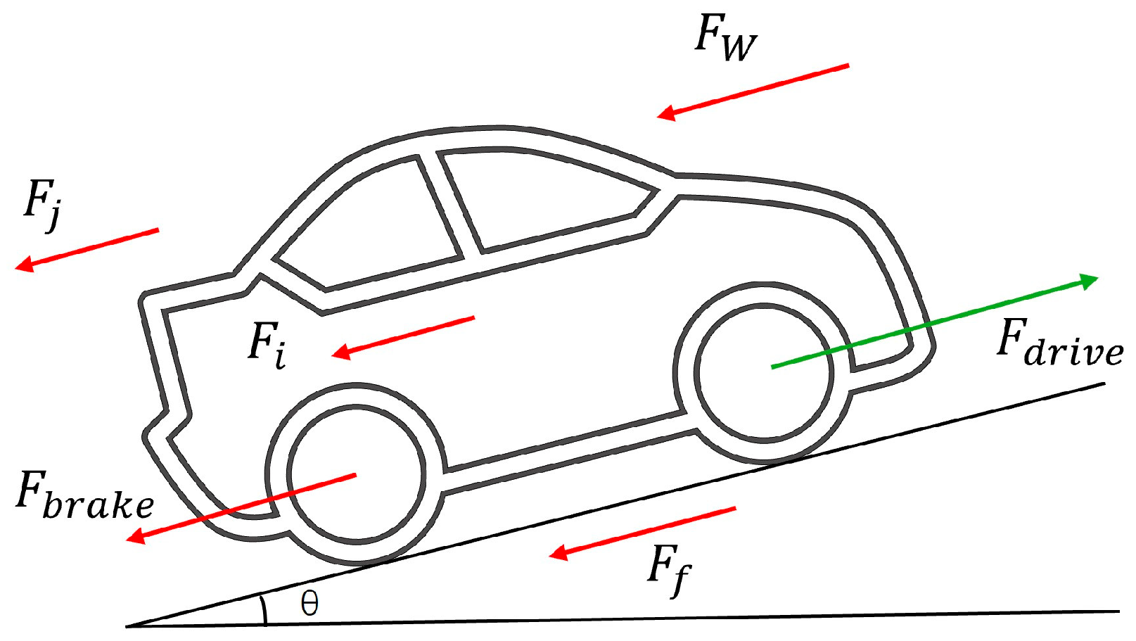
This paper constructs a longitudinal vehicle dynamics model that captures the major forces acting on the vehicle during intersection crossing. The model considers traction, rolling resistance, aerodynamic resistance, grade resistance, acceleration resistance, and braking force. Figure 3 shows the longitudinal force diagram, and the corresponding dynamic equations are expressed in Equations (1) and (2).
To quantify the traction demand of the ego vehicle at the signalized intersection, the longitudinal motion is formulated through a force-balance representation. The procedure is to write the overall equilibrium first and then decompose the total load into the main resistance and inertial components, so that the mechanical contribution of each component can be incorporated into the subsequent economy analysis.
Because the investigated maneuver may include lane changing, the motion variables used in Equations (1)–(4) are calculated from two-dimensional vehicle motion. Specifically, the longitudinal and lateral displacements are denoted by x(t) and y(t), the resultant velocity is v ( t ) = [ v x ( t ) 2 + v y ( t ) 2 ] 1 / 2 , and the resultant acceleration is a ( t ) = [ a x ( t ) 2 + a y ( t ) 2 ] 1 / 2 . The economy and comfort terms, therefore, include both longitudinal and lateral motion effects, rather than a purely one-dimensional longitudinal process.
F d r i v e = F f + F ω + F i + F j + F b r a k e
where F d r i v e is the driving force; F f is the rolling resistance; F ω is the air resistance; F i is the slope resistance; F j is the acceleration resistance; and F b r a k e is the braking force.
F f = M g f cos θ
F ω = C A u 2 21.15
C A = C D A
F i = M g sin θ
F j = M a
where M is the vehicle mass; g is the gravitational acceleration; f is the rolling resistance coefficient; θ is the road slope; C A is the air resistance coefficient; and F b r a k e is the braking force, and it is directly determined by the driver’s operation of the braking pedal.
To evaluate the economic consequences of a candidate trajectory, the propulsion demand is accumulated over the full maneuver interval. The calculation converts the instantaneous driving-power requirement into the total energy use, so that trajectories generated under different operating conditions can be compared on a unified basis.
E C = t i n t t e n d F d r i v e ( t ) v ( t ) η 0 t
where E C is the energy consumption index; η 0 is the drivetrain efficiency; and t i n t and t e n d are the initial and terminal times of the calculation interval, respectively.
The propulsion model is used here as a general traction demand approximation for comparing candidate trajectories under identical vehicle parameters. Detailed powertrain maps, regenerative braking, and vehicle-type-specific energy recovery are not considered in the present model; this simplification is acceptable for the comparative trajectory selection problem, but it also limits the direct interpretation of the economy index as a full vehicle energy management model.

3.2. Comfort Performance Metric

Riding comfort is a key indicator for evaluating vehicle operational quality and passenger experience. Traditionally, driving comfort reflects the perceptual influence of vehicle dynamic responses on occupants, which is mainly manifested by longitudinal acceleration and deceleration, lateral steering, and vertical vibration during motion. Its core objective is to ensure smooth changes in acceleration without frequent or severe jolts. At present, the quantitative characterization of driving comfort mainly depends on objective kinematic indicators. Relevant evaluation methods include vehicle ride comfort assessment approaches such as weighted root-mean-square acceleration, vibration dose value, and jerk, as well as perception mapping models derived from human vibration tolerance, which enable the multi-dimensional quantitative evaluation of riding comfort. In complex scenarios involving vehicle car following and lane changing at signalized intersections, the acceleration change rate can reflect real-time driving comfort and accurately reveal its variation characteristics.
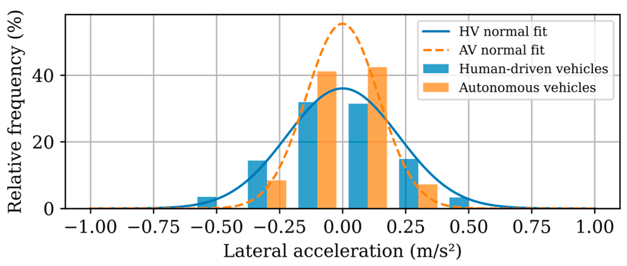
In signalized intersection scenarios, the trajectory-tracking strategy of autonomous vehicles plays a decisive role in comfort, because frequent speed adjustments and lane transitions can easily induce uncomfortable motion. To ensure smooth trajectory evolution in the proposed strategy, this paper adopts jerk as the core comfort indicator for autonomous vehicles. It represents the rate of change in acceleration and is closely related to the short-term shocks felt by passengers during braking, acceleration, and lane changing maneuvers. Other factors, such as the lateral acceleration and lane change frequency, also affect ride comfort. This paper takes jerk as the primary comfort indicator because it can intuitively reflect the smoothness of the planned trajectory and enable unified calculation for all alternative trajectories.
To match the comfort objective with the stop-and-go and lane changing characteristics of signalized intersections, the smoothness of the planned trajectory is evaluated through the jerk profile. The calculation averages the absolute jerk over the full maneuver interval, thereby capturing the cumulative longitudinal excitation experienced during the crossing process:
σ = t i n t t e n d a ˙ t d t / Δ t
where σ is the comfort index.

3.3. Efficiency Performance Metric

Vehicle efficiency is a key performance metric that reflects traffic efficiency and transportation operational quality. In this study, driving efficiency refers to the ability of the vehicle to complete its maneuver rapidly and smoothly under safety and environmental constraints. Its core objective is to reduce the travel time, idling time, and unnecessary stops. In constrained scenarios such as signalized intersections, efficiency strongly depends on the accurate prediction of signal phases and traffic flow conditions, together with the ability to update trajectories in real time.
Given the particularity of autonomous vehicles at signalized intersections, the proposed strategy divides the crossing process into three components: strategy execution, car following, and signal delay. Accordingly, the efficiency index used in this paper focuses on the total time cost of the autonomous vehicle during the full intersection-crossing process. Rather than using a single travel time measure, the model characterizes efficiency by combining the strategy completion time, vehicle following time, and signal waiting time. This three-dimensional representation enables a more comprehensive evaluation of the intersection-passing efficiency under different traffic and signal conditions.
To evaluate operational efficiency in a way that matches the temporal structure of the proposed crossing strategy, the total time cost is decomposed into its main process components. The calculation combines the durations associated with strategy execution, car-following, and signal delay, so that the time consequence of the planned maneuver can be assessed explicitly.
t t a l l = t i n t + t s t r , + t c f + t l i g
where t t a l l is the total time cost; t i n t is the initial time; t s t r , is the strategy execution time; t c f is the car following time; and t l i g is the signal delay time.

4. Area-Based Trajectory Generation Model Considering Multi-Stage Risk Avoidance

There is a strong coupling relationship between vehicle driving performance and trajectory planning. In the scenario of intelligent signalized intersections, trajectory planning for intelligent vehicles is formulated through vehicle–road–cloud interaction. The geometric shape of the trajectory determines the lateral motion characteristics and directly affects the ride comfort of the vehicle, while the vehicle motion curve determined by the trajectory governs the longitudinal dynamic response, which is related to energy consumption, driving economy, and traffic efficiency. Safety performance depends on whether the trajectory can avoid obstacles and meet road and signal constraints; efficiency performance is reflected in whether the trajectory can shorten the travel time; and economic and comfort performance require the trajectory to be smooth and continuous, with acceleration and jerk within a reasonable range. Therefore, an ideal trajectory should achieve a multi-objective balance among comfort, economy, and efficiency on the premise of safety, so as to improve the operational efficiency of intelligent intersection systems and even the entire road network.
The driving trajectory of a vehicle is the set of spatial positions and motion states that vary with time during driving. It is usually composed of the geometric path and the vehicle motion curve and serves as the final execution basis for perception, decision-making, and control in autonomous driving. In the signalized intersection scenario, the trajectory must satisfy multiple constraints: geometrically, it should fit the lane centerline without lane crossing or abrupt changes; in terms of speed, it should match the signal phase and remaining time to achieve smooth passage or safe stopping; kinematically, it requires smooth acceleration and deceleration with low jerk to ensure comfort and economy; and for safety, it needs to avoid conflicting objects such as pedestrians and vehicles while reserving sufficient safety distances. The overall trajectory should achieve multi-objective optimization among safety, efficiency, comfort, and economy.

4.1. Stage Division

To adapt the proposed area-based driving strategy to the dynamic and multi-objective characteristics of signalized intersections, the complete maneuver is decomposed into a transition phase and an adjustment phase. The transition phase describes the spatial interaction between the ego vehicle and the surrounding vehicles when lane competition or position exchange occurs, whereas the adjustment phase is used to stabilize the acquired lane position and prepare the vehicle for the subsequent control decision. This phase-based treatment reduces the computational burden, avoids consecutive aggressive lane changes, and makes the planned trajectory more compatible with the signalized intersection control logic.
To organize the multi-stage maneuver, the total longitudinal demand must first be identified before it can be distributed across phases. The calculation measures the distance between the initial planning state and the desired terminal state, thereby providing the global displacement basis for the subsequent phase division procedure.
S ( t ) = d n l o n , e g o ( t i n t + t s t a ) d n l o n , e g o ( t i n t )
where S ( t ) is the total longitudinal displacement demand; d n l o n , e g o ( t i n t + t s t a ) is the target longitudinal position at the end of the planning interval; d n l o n , e g o ( t i n t ) is the initial longitudinal position; and t i n t and t s t a are the initial planning time and the strategy execution duration, respectively.
After the total longitudinal demand is obtained, it is pre-allocated to the individual phases according to the number of remaining lane change actions. The operation transforms the global target into phase-level displacement requirements and prepares the trajectory planner for staged execution.
( d n l o n , e g o ( t i n t + t s t a ) d n l o n , e g o ( t i n t ) / n l a n )
where d n l o n , e g o ( t i n t + t s t a ) is the target longitudinal position at the end of the planning interval; d n l o n , e g o ( t i n t ) is the initial longitudinal position; and n l a n is the number of lane change actions.
Because the initial phase allocation may become inconsistent with the actual distribution of surrounding vehicles, the longitudinal target of each phase is corrected online. The operation revises the phase endpoint according to the currently available gap, so that staged planning remains feasible under dynamic traffic conditions.
d n l o n , e g o , ( t ) = d n l o n , e g o t i n t + n ( d n l o n , e g o ( t i n t + t s t a ) d n l o n , e g o ( t i n t ) / n l a n )
where d n l o n , e g o , ( t ) is the corrected longitudinal target of the n-th phase; d n l o n , e g o t i n t is the initial longitudinal position; d n l o n , e g o ( t i n t + t s t a ) is the target longitudinal position; and n is the phase index.
To support rapid trajectory generation in each phase, a dedicated execution time is assigned after the displacement target has been determined. The operation links the current phase index to the total strategy duration, thereby establishing the temporal horizon used by the staged planner.
t n s t a = ( 1 η s t r ) t s t r , ( I D s t a 1 ) , i f   n < I D s t a η s t r t s t r , , o t h e r s
where t n s t a is the execution time of the n-th phase; η s t r is the stage allocation coefficient; t s t r , is the total strategy execution time; I D s t a is the number of transition phases; and n is the current phase index.

4.2. Trajectory Generation

To improve the real-time performance and robustness of trajectory planning under the coupled objectives of safety, ride comfort, and traffic efficiency, this paper adopts a multi-stage rapid trajectory generation method. For the lane change phase, a quintic-polynomial model is used to generate smooth candidate trajectories. To simplify the planning process, the following assumptions are made: (1) because the lane change duration is short, the longitudinal velocity variation during the lane change process is neglected; (2) the longitudinal motion and lateral motion of the lane-changing vehicle are treated as independent and uncoupled; and (3) the lane change process is considered a free lane change, and the availability of the target lane is determined by the admissible gap and safety margin constraints.
The assumptions are used to keep each short lane change phase computationally tractable. They do not imply that surrounding vehicles are ignored. During execution, the terminal position of each phase is corrected according to the updated positions of surrounding vehicles, and trajectories that violate the admissible gap or longitudinal safety distance are eliminated. Therefore, the applicability of the method is limited to well-structured signalized intersection approaches with lane-level information, no pedestrian or non-motorized interference in the controlled lane changing region, and reliable short-horizon perception.
To generate smooth candidate lane change paths, the longitudinal and lateral motions are represented by quintic polynomials. The operation fits the lane change trajectory with continuous position, velocity, and acceleration profiles, so that the resulting motion remains suitable for real-time execution.
d l o n , e g o t = a 5 t 5 + a 4 t 4 + a 3 t 3 + a 2 t 2 + a 1 t + a 0
d l a t , e g o t = b 5 t 5 + b 4 t 4 + b 3 t 3 + b 2 t 2 + b 1 t + b 0
where d l o n , e g o t and d l a t , e g o t are the longitudinal and lateral displacements, and a i and b i (i = 0, 1, …, 5) are the coefficients of the quintic polynomials.
To solve the quintic-polynomial coefficients, boundary conditions must be specified at the beginning and end of the lane change maneuver. The operation constrains the lateral displacement, lateral velocity, and lateral acceleration at both endpoints, thereby ensuring a smooth start and finish for the lateral motion.
d l a t , e g o t i n t ) = d l a t , e g o ˙ t i n t = d l a t , e g o ¨ t i n t = 0
d l a t , e g o t i n t + i = 1 i = n t i s t a = W
d l a t , e g o ˙ t i n t + i = 1 i = n t i s t a = d l a t , e g o ¨ t i n t + i = 1 i = n t i s t a = 0
where i = 1 i = n t i s t a is the lane change duration within the current phase sequence, and W is the target lateral displacement.
Under the assumption that the longitudinal speed remains constant during the short lane change interval, the longitudinal travel distance can be linked directly to the maneuver duration. The operation complements the lateral boundary conditions and provides the longitudinal kinematic relation required for coefficient solving.
d l o n , e g o t i n t ) = d l o n , e g o ¨ t i n t = 0
d l o n , e g o ˙ t i n t = v i , j l o n
d l o n , e g o t i n t + i = 1 i = n t i s t a = D
d l o n , e g o t i n t + i = 1 i = n t i s t a ˙ = v i , j l o n
d l o n , e g o t i n t + i = 1 i = n t i s t a ¨ = 0
where D is the longitudinal travel distance during lane changing, and v i , j l o n is the constant longitudinal speed.
To avoid potential conflicts with surrounding vehicles, the desired longitudinal position is determined from the time-varying target vehicle that most strongly influences the ego vehicle in the current phase. The operation converts the instantaneous interaction state in the target lane into an explicit reference object for longitudinal planning.
j ( t ) | Eq.   ( 13 b )   a n d   Eq.   ( 13 c )
min d L a n I D s t a s t a , j l o n t d n l o n , e g o , t
d L a n I D s t a s t a , j l o n t d n l o n , e g o , t > 0
where j * ( t ) is the index of the target vehicle selected at time t , and d L a n I D s t a s t a , j l o n t is the longitudinal position of candidate vehicle j in the current target lane.
After the target lane vehicles are identified, the available longitudinal gap between two adjacent vehicles is evaluated. This operation measures the admissible spacing used for feasibility judgment, car following, and collision avoidance target selection.
d d L a n I D s t a s t a , j + 1 l o n ( t ) = d L a n I D s t a s t a , j l o n t d L a n I D s t a s t a , j + 1 l o n t
where d d L a n I D s t a s t a , j + 1 l o n ( t ) is the longitudinal gap between two adjacent vehicles; d L a n I D s t a s t a , j l o n t is the longitudinal position of the leading vehicle; and d L a n I D s t a s t a , j + 1 l o n t is the longitudinal position of the following vehicle.
To determine the feasible longitudinal target position within a safe gap, the desired longitudinal target is projected onto the admissible interval bounded by the two adjacent vehicles and the required safety margin. The operation selects the feasible position closest to the desired target, thereby retaining the original planning intention as far as possible under the safety constraint.
d n l o n , e g o ( t ) = d L a n I D s t a s t a , j l o n t ( t e x p v L a n I D s t a s t a , j l o n ( t ) + 0.6 l v e h )
where d n l o n , e g o ( t ) is the corrected longitudinal target position; d L a n I D s t a s t a , j * * l o n t is the longitudinal position of the rear-boundary vehicle; t e x p is the desired time headway; v L a n I D s t a s t a , j * * l o n ( t ) is the speed of the boundary vehicle; and l v e h is the vehicle length.
When the desired longitudinal position falls ahead of the feasible interval, it is projected onto the front boundary of the admissible gap. The operation preserves the safe following requirement while keeping the corrected target as close as possible to the original planning intention.
d n l o n , e g o ( t ) = d L a n I D s t a s t a , j + 1 l o n t + ( t e x p v L a n I D s t a s t a , j l o n + 0.6 l v e h )
The set of vehicles that must be overtaken in the k-th phase is identified by selecting the surrounding vehicles whose lateral positions fall within the lateral region of the current phase and whose longitudinal positions lie inside the corresponding phase interval ahead of the ego vehicle.
After the overtaken vehicle set and the nearest following reference vehicle are identified, the lateral terminal position of the current phase is determined. The operation subtracts the lateral safety allowance from the reference configuration, thereby converting the local interaction state into an explicit lateral planning target:
d n l a t , e g o ( t ) = m i n { d L a n I D s t a s t a , n l a t t d l a t , e g o t 1.2 l w } , n { k 1 , j + 1 }
where d n l a t , e g o is the lateral target position of the ego vehicle; d L a n I D s t a s t a , n l o n is the lateral position of the reference vehicle; d l a t , e g o is the current lateral position of the ego vehicle; l w is the vehicle width; and n { k 1 ,     j + 1 } denotes the candidate vehicles considered in the current phase.

4.3. Trajectory Adjustment

In the proposed strategy, the desired terminal position of each phase is first determined under the ideal assumption that surrounding vehicles travel at a constant speed. This assumption simplifies the initial phase planning and enables the rapid generation of candidate trajectories. In actual traffic, however, surrounding vehicles rarely maintain strict constant-speed motion, and the real interaction gaps gradually deviate from their pre-planned values as the maneuver progresses.
Because the pre-planned phase endpoint may deviate from the actual traffic state as surrounding vehicles move, the trajectory must be corrected online during strategy execution. The operation first updates the terminal position of the current phase and then regenerates the trajectory from the current state to the corrected endpoint, so that the planned passing order can be maintained under dynamic traffic conditions.
It should be noted that the mathematical symbol system formulated in this study is specifically tailored to lane-level scenario simulation modeling, which is confined to the scope of the established modeling framework. The variable symbols used in Table 1 consist of three parts: the main symbol, superscript, and subscript. The main symbol represents the core physical meaning of a variable, the superscript defines variable attributes and specifies relevant constraints, and the subscript acts as a mathematical identifier to reflect the mathematical definition and quantitative implications of the variable. Taking d n l o n , e g o as an example, the main symbol d denotes the physical quantity of displacement; the superscript l o n , e g o defines this displacement as the longitudinal displacement of the ego vehicle; and the subscript n refers to the vehicle serial number.

5. Area-Based Multi-Objective Driving Strategy for Autonomous Vehicles

5.1. Strategy Framework

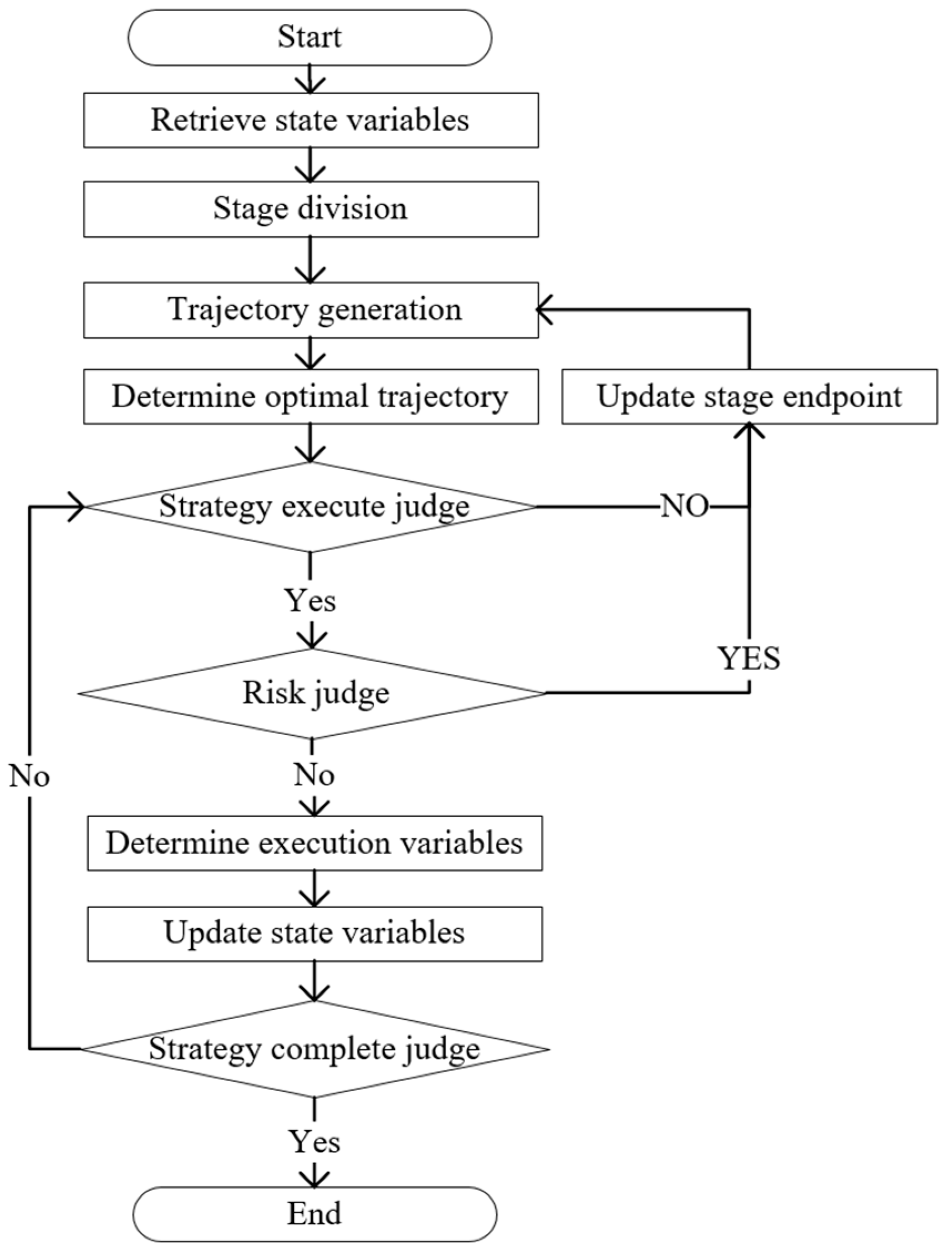
As shown in Figure 4, this paper presents an area-based driving strategy for autonomous vehicles at signalized intersections. Upon entering the strategy execution zone, the vehicle acquires real-time traffic and lane information and predicts the positions of surrounding vehicles under constant-speed motion within the strategy execution time window to select suitable car following targets. The trajectory is then divided into several crossing stages and one correction stage according to the number of lanes to be crossed and the surrounding vehicle distribution, with the start and end points of each stage determined sequentially under safety constraints. In the longitudinal direction, target longitudinal positions satisfying safety criteria are searched based on equally spaced points along the lane change distance, considering the desired time headway and safety distance. In the lateral direction, the lateral displacement is determined by subtracting the vehicle width from the minimum lateral offset between the ego vehicle and the vehicles to be passed at each stage, with transitional positions between lanes preset at the end of each stage. Real-time risk monitoring is performed throughout trajectory generation. Collision risks are detected by evaluating the lateral and longitudinal overlaps between the ego vehicle and preceding vehicles; trajectories violating safety conditions are directly eliminated. If no feasible trajectory meets the safety and passing requirements, the proposed strategy is terminated, and the vehicle reverts to car following. Finally, the correction stage smoothly regulates the vehicle to the center of the target lane and maintains car following behind the target vehicle. All feasible trajectories are evaluated via simulation in terms of passing performance, and the optimal trajectory is selected with the corresponding control acceleration to achieve the safe and efficient traversal of autonomous vehicles through signalized intersections.
To accurately satisfy the optimization objectives of vehicle comprehensive performance, this study adopts the vehicle dynamic model established in Equations (6)–(17) to describe the sub-second lateral and longitudinal dynamic responses of vehicles during driving. In the modeling process, secondary interference factors such as external disturbances, tire wear, and transmission vibration are neglected to simplify the model and highlight core motion characteristics. Meanwhile, the Intelligent Driver Model (IDM) is applied to characterize human driving behaviors, and all drivers are assumed to be homogeneous. Generally, high-precision motion prediction inevitably brings a heavy computational burden. Given that the proposed strategy possesses favorable anti-interference capabilities and can cope with unstable operating conditions, it has a minor dependence on prediction accuracy. Accordingly, the uniform motion hypothesis, with a lower computational cost and better real-time performance, is adopted for prediction, which effectively reduces the overall computational load while guaranteeing the stability of the proposed strategy.

5.2. Objective Function

To select the optimal candidate trajectory from the viewpoints of economy, comfort, and efficiency, a unified cost function is constructed. The operation combines the three performance terms into a single optimization objective, thereby allowing the planner to evaluate different candidate trajectories within one decision framework.
To construct a balanced comprehensive objective function that takes economy, comfort, and efficiency into account, magnitude unification is first performed on the three types of evaluation indicators; this is only applicable to scenarios where equal weights are assigned to all indicators. Combined with the typical value ranges of each indicator obtained from benchmark simulations, three sets of fixed scaling coefficients are determined for magnitude normalization. These coefficients remain constant across all candidate trajectories and test scenarios to ensure that the normalized values of the three indicators are at a similar magnitude level. The normalized indicators are summed up to establish the balanced objective function with equal priority, so as to realize multi-objective balanced optimization. In weight allocation scenarios focusing on a single performance indicator, the original indicator values can be directly adopted without magnitude unification. This is because scaling a single indicator with fixed constants cannot alter the ranking of candidate trajectories and thus exerts no substantial influence on the optimization results.
m i n ω 1 E E C + ω 2 C σ + ω 3 T t t a l l
where E C is the economy term; σ is the comfort term; t t a l l is the efficiency term; E * denotes the normalization coefficient of economy with a value of 19.1571; C * represents the normalization coefficient of comfort with a value of 5.3996; and T * stands for the normalization coefficient of efficiency with a value of 0.02833. It is noted that E * can be calculated via benchmark group experiments, as shown in Section 6.2.2.
This paper adopts the fixed-magnitude scaling method adapted to the [1, 1, 1] equilibrium condition for data preprocessing, obtains normalization coefficients to unify the magnitudes of the three indicators, and avoids optimization deviations caused by magnitude differences.
It is noted that the core focus of this research is to explore the internal mechanism of the multi-objective collaborative optimization of automated vehicles for diverse performance demands, and the adopted data processing method can effectively reveal the evolution laws of various performance indicators. From the perspective of practical application, automated vehicles can independently assign objective weights in actual operating scenarios, so as to accurately match differentiated performance requirements under various working conditions. The weighted-sum objective function established in this paper is a performance evaluation framework tailored to specific application scenarios, rather than a rigorous Pareto-optimal multi-criteria optimization system. As the accurate calibration of the Pareto front has not been fulfilled in this study, the analytical results derived from weight assignment can only reflect the evolutionary characteristics of system performance under preset decision preferences, and they cannot be adopted as universally applicable global optimal trade-off strategies.

5.3. Constraints

To ensure the feasibility and safety of the generated trajectory, this paper establishes corresponding constraints. On the one hand, physical constraints including vehicle dynamic limits, road boundaries, and traffic signal control are satisfied to ensure that the trajectory conforms to vehicle motion characteristics and traffic regulations. On the other hand, safety constraints such as safe spacing, collision avoidance, position, and velocity boundaries are adopted to prevent potential hazards in the complex intersection environment. Meanwhile, these constraints provide a feasible solution space for the multi-objective optimization problem, thus guaranteeing the stable convergence and rationality of the algorithm.
Vehicle dynamic constraints conform to the inherent motion characteristics and mechanical limits of vehicles, effectively guaranteeing the physical feasibility of the planned driving trajectories. These constraints are mainly presented in Equations (1)–(2d). The piecewise constraints formulated for driving strategies under signalized intersection scenarios divide control rules according to different driving phases, standardize the operating states and adjustment logic of vehicles in different driving intervals, and enable the overall driving strategy to better adapt to the traffic timing characteristics at intersections; they are shown in Equations (6)–(9). The various boundary and operational constraints established in the trajectory generation stage define the feasible range of trajectory planning from the perspectives of the driving space, operating state, and travel sequence. Such constraints can avoid illegal driving behaviors and potential collision risks and further improve the rationality and safety of planned trajectories. All the above constraint relations are fully expressed and strictly restricted in Equations (10a)–(17).
To determine whether the current phase is being executed as expected, the actual longitudinal position of the ego vehicle is compared with the desired position specified for that phase. The operation produces a stage decision variable that supports phase transition judgment and terminal-state updating during online execution.
χ ( t ) = 1 ,     i f   d l o n , e g o ( t ) d I D s t a l o n , e g o t 2 ,     i f   d l o n , e g o ( t ) > d I D s t a l o n , e g o t
where χ ( t ) is the stage decision variable; d l o n , e g o ( t ) is the actual longitudinal position of the ego vehicle; and d I D s t a l o n , e g o t is the desired longitudinal position specified for the current phase.
To guarantee collision-free car following during the maneuver, the admissible longitudinal spacing behind the preceding vehicle must be evaluated explicitly. The operation calculates the minimum safety distance from the current speed condition, braking capabilities, and static safety margin, thereby providing a safety screening criterion for candidate trajectories.
d s a f e ( t ) = v I D s t a l o n , e g o 2 ( t ) v I D s t a 1 l o n 2 ( t ) 2 g μ + d m i n
where d s a f e is the minimum longitudinal safety distance; v I D s t a l o n , e g o is the speed of the ego vehicle; v I D s t a 1 l o n is the speed of the preceding vehicle; g is gravitational acceleration; μ is the road adhesion coefficient; and d m i n is the static safety margin.

5.4. Strategy Solving Algorithm

In the actual execution process, optimization solution is realized through the dynamic selection of limited candidate trajectories. Within each planning step, feasible candidate trajectories are generated in accordance with phased lane changing rules; infeasible candidate trajectories are eliminated by constraints; the remaining candidate trajectories are evaluated via the objective function; and the trajectory with the lowest cost is selected in the end. The search process terminates when all candidate terminal states within the current planning area have been evaluated or no feasible trajectories remain. It can be concluded from the above analysis that the driving behavior and multi-performance collaborative optimization problem of automated vehicles at signalized intersections present obvious strong nonlinearity, so it is difficult to obtain rigorous analytical solutions through theoretical derivation. Accordingly, this study adopts the dynamic programming algorithm to solve the numerical solutions of the model, so as to effectively approximate the theoretical analytical solutions. The strategy solving algorithm is outlined in Algorithm 1.
Algorithm 1
Note:
(1) Input variables: v ( t i n t ), d ( t i n t ), a ( t i n t );
(2) Output variables: a(t);
(3) Risk variables and decision variables: χ ( t )
Input: Initial vehicle states v ( t i n t ), d ( t i n t ), a ( t i n t ); signal phase and timing at t = 0
Output: Optimal longitudinal trajectory and control command
Initialize t → 0
Obtain intersection information: vehicle states {v, d, a} and signal phase
 
Initialize the stage flag and optimal trajectory
If the vehicle is at the strategy departure time, then
 Step 1: Calculate desired position via Equation (13a–c)
 Step 2: Implement phase division via Equations (6)–(9)
 Step 3: Generate candidate trajectories via Equations (10a)–(12e) and Equations (14)–(17)
   Evaluate performance of feasible trajectories via Equations (3)–(5)
 Step 4: Select the optimal trajectory via Equation (18)
 Step 5: Judge stage decision variable via Equation (19); if χ ( t ) = 1 , update the stage endpoint, go to Step 3; otherwise, risk variable judgment; if yes endpoint update, go to Step 3; otherwise, go to Step 6
 Step 6: Determine execution variable at time t
 Step 7: Time iteration: t ← t + tt
 Step 8: Strategic variable judgment Equation (19); if χ ( t ) > 1 , go to Step 5; otherwise, end loop
It is noted that the dynamic programming-based solution method proposed in this study is only validated in simulated scenarios and remains at the stage of simulation research. Although this method exhibits favorable anti-interference capabilities, further standardization of the iteration termination criteria and state transition rules is essential for its practical engineering application. In addition, practical constraints including computational complexity, perception uncertainty, and communication delays should be fully taken into account in the application.

6. Results and Discussion

Numerical experiments are conducted from three perspectives: strategy-related factors, system-side factors, and application adaptability. Strategy-related factors include objective weights. System-side factors include the traffic demand, green time ratio, and strategy trigger region length. Application adaptability factors include the AV penetration rate, allowable lane changing gap, benchmark strategy, and sudden information disturbances.
In addition, other factors that generate auxiliary disturbances are analyzed qualitatively. The simulation parameters can be seen in Table 2 [24,25,26]. This simulation calculation is carried out on the MATLAB platform (R2023a) [24]. Vehicles are generated in accordance with preset traffic flow volumes, and vehicle movement trajectories are measured under consistent conditions in terms of road length, split ratio, strategy trigger interval length, and vehicle parameters.
It is worth noting that the conclusions drawn in this study are only applicable to standardized and simplified simulation scenarios. The proposed model fails to take real traffic elements into account, including pedestrians, non-motor vehicles, lateral traffic flows, and diverse driving behaviors. Accordingly, the research results only verify the effectiveness of the proposed method under ideal and controllable conditions. In future studies, relevant practical factors will be comprehensively considered to provide theoretical support for its practical engineering application.

6.1. Strategy Weight Sensitivity Analysis

This section evaluates the performance sensitivity of the proposed trajectory optimization method in terms of economy, comfort, and efficiency. It then analyzes the feasibility and scenario adaptability of the proposed strategy in signalized intersection environments.
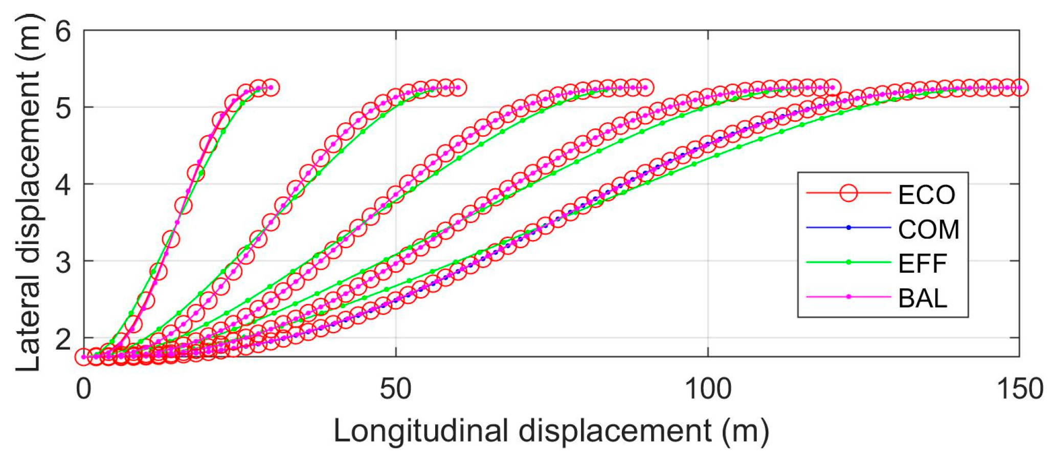
In the signalized intersection trajectory planning strategy proposed in this paper, the vehicle’s traffic economy, efficiency, and ride comfort are primarily determined by the longitudinal travel displacement, longitudinal travel velocity, and lateral displacement. Among these, the longitudinal displacement and velocity directly influence the vehicle’s intersection passing efficiency and longitudinal safety distance, while the lateral displacement governs the lane changing amplitude and lateral safety clearance. Indicators such as vehicle acceleration, trajectory curvature, and collision risk can all be derived from the above three variables. Therefore, selecting the longitudinal displacement, longitudinal velocity, and lateral displacement as sensitivity analysis variables enables the comprehensive characterization of the variation patterns in trajectory planning performance. To investigate the performance sensitivity of the trajectory optimization method, the weight coefficients of the objective function are sequentially set to [1, 0, 0], [0, 1, 0], [0, 0, 1], and [1, 1, 1], yielding the optimal trajectories oriented toward economy, comfort, and efficiency under different driving demands, respectively. Hence, the economic trajectory (ECO), comfort trajectory (COM), efficiency trajectory (EFF), and balanced trajectory (BAL) can be obtained.
The effects of the longitudinal displacement demand on economy, comfort, and efficiency are examined and can be seen in Figure 5 and Table 3. The three types of vehicle performance trajectories exhibit distinct performance differentiation under various longitudinal displacement demands. The economic trajectory and comfort trajectory show highly consistent performance in terms of energy consumption and acceleration fluctuation: the longitudinal displacement demand increases from 30 m to 150 m and the energy consumption of both trajectories decreases from 6.6 to 0.63, while the acceleration fluctuation drops from 21 to 0.19 and the completion time increases linearly with the displacement (1.5–1.6 s for 30 m and 7.5 s for 150 m). This reflects smooth, low-energy-consumption operation, reflecting the design foci of the two trajectories on economy and comfort, respectively. In contrast, the efficiency trajectory takes maximum-speed driving as its core objective, possessing a significant advantage in terms of completion time. Under the same displacement demand, the completion time of the efficiency trajectory is only approximately two-thirds of that of the economic/comfort trajectories (e.g., for 150 m displacement, the efficiency trajectory takes 5 s, far less than the 7.5 s of the economic/comfort trajectories). However, this advantage comes at the cost of drastically increased energy consumption and acceleration fluctuations: at 150 m displacement, the energy consumption of the efficiency trajectory (8.8) is about 14 times that of the economic/comfort trajectories (0.63), and the acceleration fluctuation (9.0) is approximately 47 times that of the latter (0.19), clearly verifying its efficiency orientation. In summary, the three trajectories form clear performance preferences in the dimensions of economy, comfort, and efficiency. The economic and comfort trajectories achieve low energy consumption and low impacts through gentle acceleration and deceleration, while the efficiency trajectory reduces the completion time via limited acceleration/deceleration and maximum-speed driving. These results validate that the proposed strategy can generate longitudinal driving trajectories oriented toward corresponding performance objectives according to specific demands.
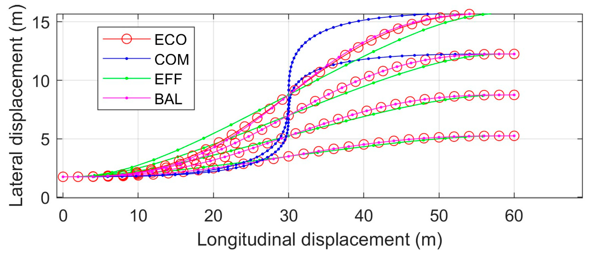
The effects of the lateral displacement demand on the three performance dimensions are investigated. According to Figure 6 and Table 4, the three types of vehicle performance trajectories exhibit distinct performance differentiation in terms of energy consumption, acceleration fluctuation, and completion time under various lateral displacement demands. The economic trajectory consistently maintains low energy consumption and relatively stable acceleration fluctuation: as the lateral displacement demand increases from 3.5 m to 14 m, the energy consumption rises gradually from 2.0 to 6.4, the acceleration fluctuation increases from 2.8 to 9.3, and the completion time only increases slowly from 3 s to 3.3 s. This reflects a design focus centered on low energy consumption while balancing driving stability, verifying its economic orientation. The comfort trajectory prioritizes the suppression of acceleration fluctuations as its core objective: at a lateral displacement demand of 3.5 m, its acceleration fluctuation (2.47) is slightly lower than that of the economic trajectory (2.8); as the displacement demand increases to 14 m, the acceleration fluctuation only rises slightly to 6.0, which is significantly lower than the 9.3 of the economic trajectory at the same displacement. Meanwhile, the completion time is notably prolonged with increasing displacement (reaching 6.4 s at both 10.5 m and 14 m), verifying its comfort orientation. The efficiency trajectory takes maximum-speed driving as its core, possessing an absolute advantage in terms of completion time: the completion time remains stable at 2 s under all lateral displacement demands, far shorter than those of the economic and comfort trajectories. However, this advantage comes at the cost of drastically increased energy consumption and acceleration fluctuations—at 14 m displacement, the energy consumption of the efficiency trajectory (26) is approximately 4.1 times that of the economic trajectory (6.4) and 3.0 times that of the comfort trajectory (8.7), while its acceleration fluctuation (65) is about 7.0 times that of the economic trajectory (9.3) and 10.8 times that of the comfort trajectory (6.0). In summary, the three trajectories form clear performance preferences in the dimensions of economy, comfort, and efficiency. The economic trajectory achieves low energy consumption through gentle acceleration and deceleration, the comfort trajectory enhances ride comfort by extending the driving time to suppress acceleration fluctuations, and the efficiency trajectory reduces the completion time via limited acceleration/deceleration and maximum-speed driving. These results validate that the proposed strategy can generate vehicle driving trajectories oriented toward corresponding performance objectives according to the lateral displacement demand.

6.2. Analysis of Main Factors of the Intelligent Transportation System

Under the vehicle–road–cloud integrated architecture, the road traffic flow, green signal ratio, and strategy trigger region length are the primary representative key parameters at the vehicle, road, and cloud levels, respectively [18,20,22]. The coupling of these three parameters determines the scenario adaptability and robustness of the strategy, and they constitute the direct external factors affecting the operational efficiency of the system. In this section, a quantitative analysis is carried out on the above three types of parameters, while qualitative supplements are provided for other environmental and information-related factors.

6.2.1. Impacts of Vehicle Factors on the Strategy

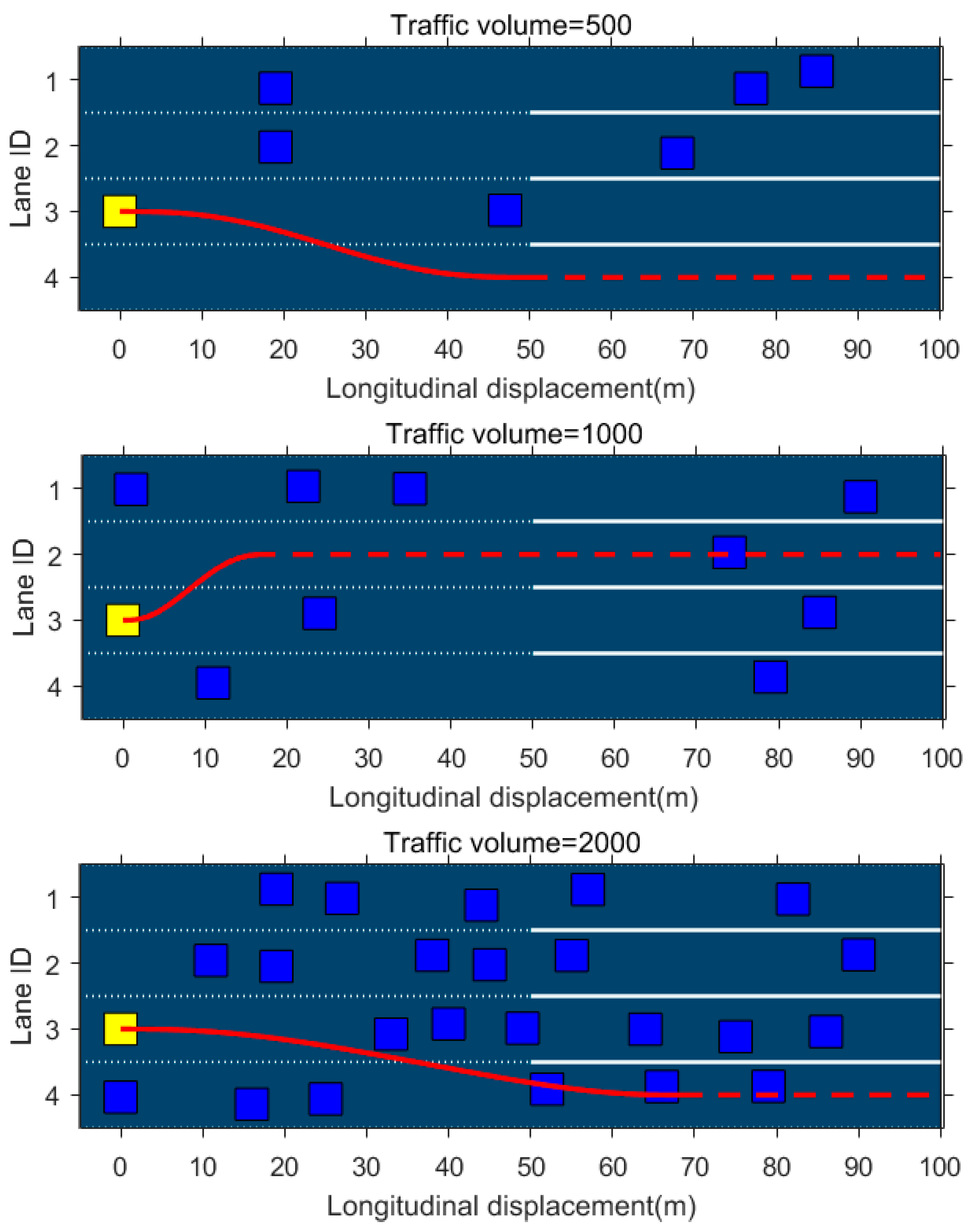
To examine the impacts of vehicle factors on the strategy, the objective function weights are set to [1, 1, 1], and the proposed strategy is evaluated under different traffic demands. Road traffic flow directly reflects the traffic load and vehicle interaction intensity and is the most critical vehicle-side factor affecting driving smoothness, energy consumption, and traffic efficiency. In this paper, three levels of traffic flow, 500, 1000, and 2000 veh/h, are set for comparison. The following tables summarize the available simulation outputs reported in the current work.
Regarding the influence of the traffic demand (seen in Table 5), as the traffic volume increases from 500 veh/h to 2000 veh/h, the economy indicator rises from 0.0361 to 0.0457, and the energy consumption performance gradually deteriorates with increasing traffic densities. The comfort indicator reaches 0.125 at 1000 veh/h, which is significantly higher than that at 500 veh/h (0.0402) and 2000 veh/h (0.0441), indicating frequent vehicle interactions and intensified acceleration/deceleration shocks under a medium traffic flow, leading to degraded ride smoothness. The efficiency indicator remains stable at 35.2–35.3 in the range of 500–1000 veh/h and increases to 40.1 at 2000 veh/h. Congestion tends to emerge under high traffic flows, reducing the traffic efficiency. The detailed trajectories can be seen in Figure 7.
The results indicate that, under a low traffic flow, economy and comfort are optimal while efficiency remains stable; under a medium traffic flow, vehicle interactions become frequent, and comfort decreases significantly; under a high traffic flow, congestion intensifies and both economy and efficiency deteriorate synchronously. The overall performance of the strategy tends to be more conservative with increasing road traffic flows. Besides traffic flow, other vehicle factors, such as the vehicle type, speed distribution, and car-following behavior discrepancies, also exert influences; they increase acceleration fluctuations and energy consumption dispersion but do not alter the dominant effect of traffic flow on the overall performance.

6.2.2. Impacts of Road Factors on the Strategy

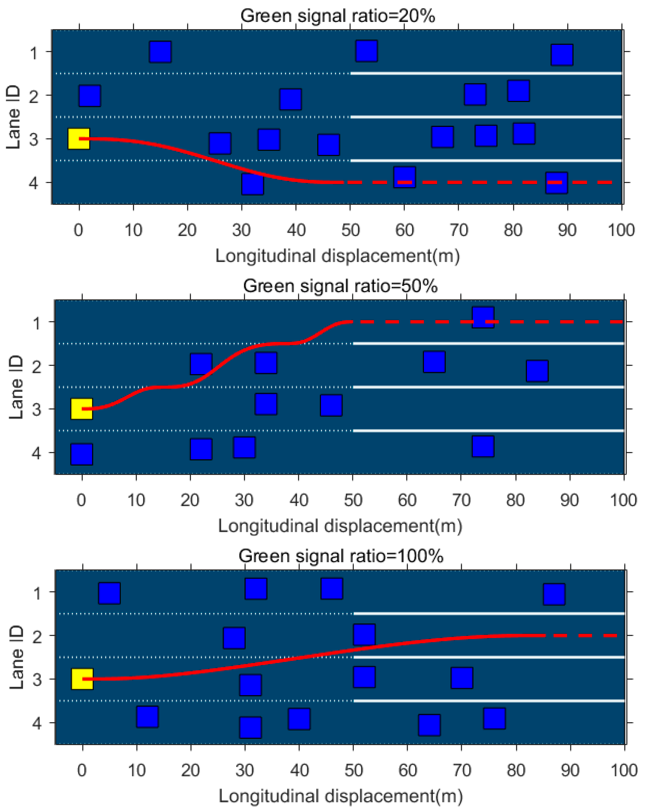
The green signal ratio determines the effective passage time window at intersections, directly governs vehicle start–stop behavior and traffic efficiency, and is the most critical road factor affecting road resource utilization. In this paper, simulations are carried out with three levels of green signal ratio: 20%, 50%, and 100%. The green signal ratio directly determines vehicle start–stop operations and traffic efficiency (as seen in Table 6).
The economic performance is optimal (0.0192) at a 20% green signal ratio, with values of 0.0522 and 0.0502 at 50% and 100%, respectively. A higher green signal ratio increases idle and braking events, elevating the energy consumption. Comfort is best at 20% (0.0272) and worst at 50% (0.185), as frequent acceleration and deceleration occur under a medium green signal ratio. Efficiency improves markedly with an increase in the green signal ratio, with the indicator dropping from 55.3 at 20% to 7.4 at 100%. A longer green light duration substantially reduces waiting times and enhances road traffic efficiency. The detailed trajectories can be seen in Figure 8.
The results show that the lower the green signal ratio, the worse the efficiency but the better the economy and comfort; at a medium green signal ratio, frequent acceleration and deceleration result in the worst comfort. The higher the green signal ratio, the higher the traffic efficiency, accompanied by increased energy consumption and fluctuations. The green signal ratio is positively correlated with efficiency and negatively correlated with economy and comfort. In addition to the green signal ratio, other road control factors, such as the signal cycle, phase sequence, and queue clearance length, also exert impacts that alter the temporal constraints of the trajectory, yet they do not change the dominant effect of the green signal ratio on traffic efficiency.

6.2.3. Impacts of Cloud Factors on the Strategy

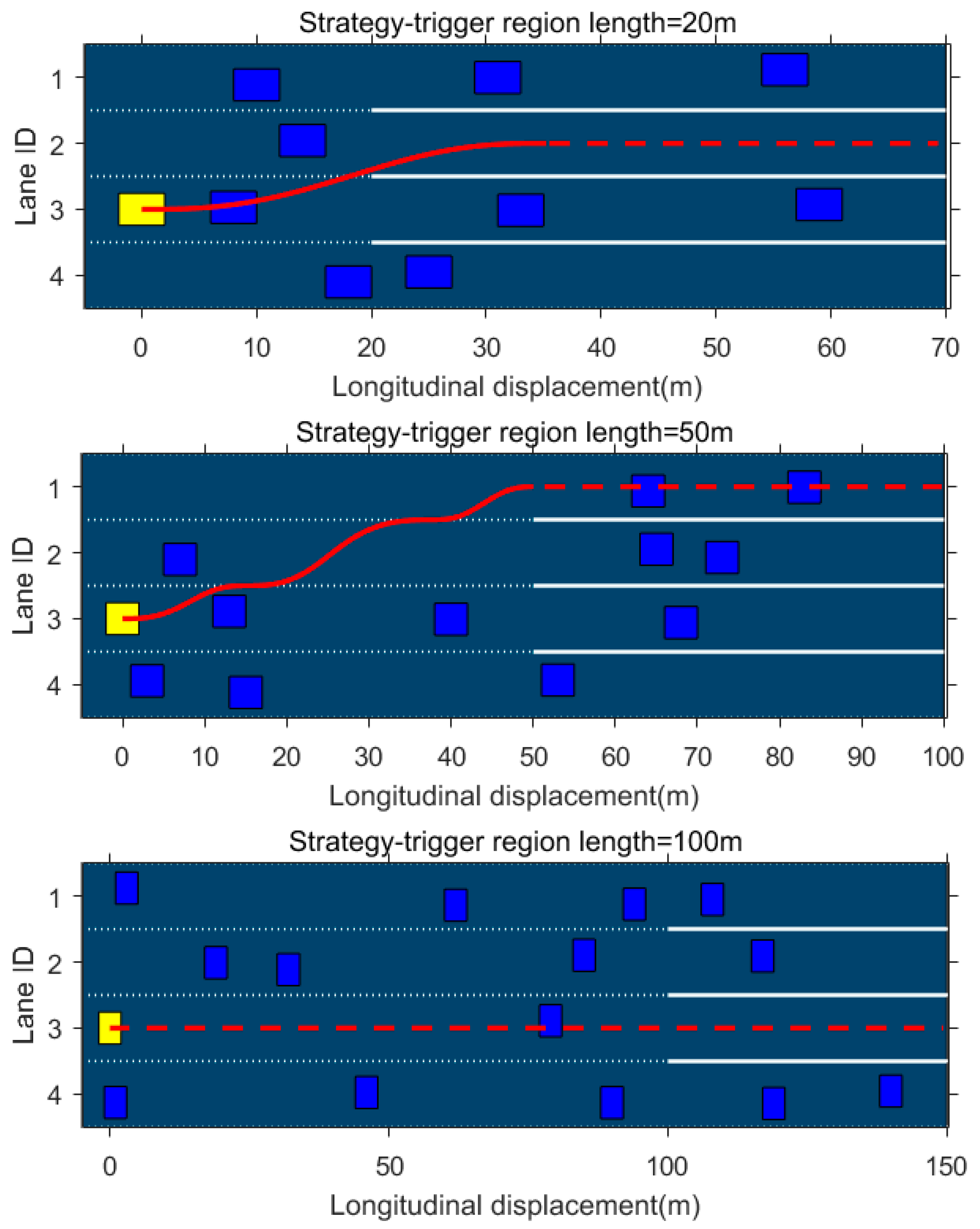
The length of the strategy triggering region determines the trajectory pre-optimization space and lane changing feasibility and directly governs the lead and smoothness of cloud-side global planning. It serves as the most critical cloud element affecting the cooperative performance. In this paper, three length levels of 20 m, 50 m, and 100 m are set for comparative analysis.
The length of the lane change zone exerts a significant impact on all performance indicators (seen in Table 7). The economy indicator at 50 m is 0.0522, worse than that at 20 m (0.0198) and 100 m (0.0268). A medium-length lane change zone tends to trigger frequent lane changes, raising the energy consumption costs. The comfort indicator peaks at 0.185 for 50 m, much higher than those for 20 m and 100 m. The 100 m lane change zone achieves the best comfort (0.0266), suggesting that sufficient lane change space effectively reduces driving shocks. The efficiency indicators are 37.2 and 37.3 for 20 m and 100 m, respectively, and 35.3 for 50 m, demonstrating that a moderate lane change zone length helps to improve the overall traffic efficiency. The detailed trajectories can be seen in Figure 9.
The results indicate that a short interval leads to insufficient planning space; a medium interval brings frequent lane changes, achieving the optimal efficiency but the worst comfort; and a long interval enables sufficient planning, delivering the optimal smoothness and economy with stable efficiency. Appropriately expanding the regional length contributes to an improvement in comprehensive performance. In addition to the regional length, cloud elements such as communication delays, the calculation frequency, and the perception range also exert certain impacts. An increase in delay will reduce trajectory reliability, yet it cannot change the leading role of the region length in planning quality.

6.3. Analysis of Application Adaptability of the Strategy

In the mixed traffic scenario with automated vehicles at signalized intersections, the automated vehicle penetration rate, allowable lane changing gap, mainstream control strategies, and sudden disturbances in traffic information are the most representative core influencing factors in terms of traffic composition, driving behavior, strategy comparison, and information transmission, respectively. These four types of factors determine the adaptability and robustness of the proposed optimization strategy under complex intersection traffic conditions, and they serve as key indicators to evaluate the engineering practicability and scenario applicability of the strategy. In this section, a systematic quantitative simulation analysis is conducted on the above key parameters to explore the influence rules of parameter fluctuations on the multi-performance optimization effect of the strategy. In the subsequent simulation experiments, vehicles entering the system are generated by stochastic functions to guarantee the randomness of the traffic flow distribution. The traffic flow is set to 1000 vehicles per hour, the length of the variable lane area is 50 m, the green light timing ratio is set to 50%, and the weights of all performance indicators are uniformly defined as [1, 1, 1] [23,24,25].
It should be noted that the simulation scenario constructed in this paper is theoretical. Reasonable assumptions are adopted to highlight the coupling effects of vehicle, road, and cloud elements, which jointly form complex real-world traffic scenarios. Accordingly, the simulation analysis under such assumptions can effectively explore the application effects and feasibility of the proposed strategy in practical working conditions.

6.3.1. Influence of Penetration Rate on Strategy Application

This simulation experiment aims to explore the influence law of the automated vehicle penetration rate on various traffic performance aspects of the proposed strategy. In the simulation, the traffic flow is set to 1000 veh/h, the length of the lane change area is 50 m, the green signal ratio is set to 50%, and the weight of each performance objective is uniformly defined as [1, 1, 1]. The total simulation duration is fixed at 1 h. The penetration rate of automated vehicles increases gradually from 0% to 100% with an interval of 2%. To ensure the reliability of the simulation results, 16 independent, repeated simulations are conducted under each penetration rate condition, and a total of 816 groups of traffic flow statistical samples are obtained. Each sample value in the box plot represents the average performance of all automated vehicles and human-driven vehicles in a single simulation, which can directly reflect the evolution characteristics of the overall traffic performance in mixed traffic flows.
All four evaluation indicators adopted in this study are cost-type indicators, where a smaller value indicates better corresponding performance. Specifically, the economic indicator characterizes the energy consumption cost per unit driving distance; the comfort indicator is quantified based on parameters related to the acceleration variation rate; the efficiency indicator measures the time cost for vehicles to pass through signalized intersections; and the comprehensive performance indicator is obtained by summing the economic, comfort, and efficiency indicators.
The comprehensive performance consists of three cost components: economy, comfort, and efficiency. As shown in Figure 10, the comprehensive index rises from 35.0 at a 0% penetration rate to approximately 37.4 near the 10% penetration rate, representing an increase of around 6.9%, which clearly reflects a brief negative response under mixed traffic conditions with low penetration rates. Afterwards, the comprehensive index keeps declining as the penetration rate grows, registering 32.6, 28.4, and 26.2 at penetration rates of 30%, 50%, and 70% respectively, and dropping to 24.6 at the 100% penetration rate—a reduction of roughly 29.7% compared with the 0% penetration rate. Since the current comprehensive index is calculated by directly summing the three indicators, and the absolute value of the efficiency indicator is relatively large, the overall trend in comprehensive performance is similar to the variation in efficiency. Nevertheless, the simultaneous improvement in economy and comfort further intensifies the downward trend. The comprehensive index only fluctuates slightly at high penetration rates, indicating that, when most vehicles adopt similar trajectory optimization logic, the system operating state gradually stabilizes, and the performance improvement shifts from rapid enhancement to diminishing marginal returns.
Overall, the simulation results can be divided into three stages. In the low penetration rate range of 0% to 10%, a small number of automated vehicles fail to form stable group coordination, and behavioral differences between automated and human-driven vehicles may cause local car following disturbances, leading to varying degrees of increases in all four indicators. In the range of approximately 10% to 60%, the rising proportion of automated vehicles enables candidate trajectory optimization, safety gap screening, and unified control to gradually produce group effects, which significantly improve the economic efficiency, driving comfort, traffic efficiency, and comprehensive performance. In the medium-to-high penetration rate range of 60% to 100%, the four indicators keep decreasing, with a gradually narrowed improvement range and slight random fluctuations, indicating that the traffic flow has gradually reached a stable operating state.

6.3.2. Influence of Lane Changing Factors on Strategy Application

This simulation is conducted to explore how the lane changing activity of human-driven vehicles affects the implementation effects of the proposed intelligent driving strategy and group operational performance at signalized intersections. Human-driven vehicles can obtain the headway distances to the preceding vehicles in the current lane, left adjacent lane, and right adjacent lane in real time and judge whether to change lanes according to the difference between the forward headway of adjacent lanes and that of the current lane. When the difference exceeds the threshold, the vehicle will perform lane changing toward the adjacent lane with a larger gap. Accordingly, the threshold characterizes the lane changing prudence of human-driven vehicles: a smaller value means more frequent lane changing behaviors, while a larger value indicates more conservative lane changing decisions. The simulation environment remains consistent with that described in Section 6.3.1. The threshold a is set to vary from 0 m to 150 m at an interval of 10 m, forming 16 working conditions in total, and 12 independent repeated simulations are carried out for each condition. The output results presented in Figure 11 cover the trajectory planning success rate, the trajectory completion degree, and variations in the comprehensive performance of automated vehicles, which can reflect the overall response characteristics of a mixed traffic flow.
As the lane changing threshold of human-driven vehicles increases from 0 m to 150 m, the number of lane changes among human-driven vehicles drops significantly from 4059.8 to 99.3. Meanwhile, the trajectory success rate of autonomous vehicles rises from 77.5% to 95.2%, and the trajectory completion rate grows from 84.9% to 97.6%. The group economic efficiency, comfort, efficiency, and comprehensive performance all show a declining trend as a increases, among which the comprehensive performance falls from 30.6 to 25.5. The results indicate that overly aggressive lane changes by human-driven vehicles will undermine the target lane stability of autonomous vehicles, reduce the success rate of trajectory execution, and raise the overall operating cost of the vehicle group. Increasing the lane changing threshold can effectively alleviate this issue; however, in the high threshold range, the magnitude of performance improvement gradually diminishes and levels off.
When a is small, human-driven vehicles frequently change lanes due to minor advantages in forward spacing, leading to the constant restructuring of the lane occupancy relationships within the local traffic flow. For autonomous vehicles, such frequent lane changes continuously alter the positions of preceding vehicles, available insertion gaps, and potential conflict relationships in the target lane. Consequently, autonomous vehicles more often encounter failed safety screening, trajectory interruptions, or strategy revision during candidate trajectory searching. The additional speed adjustments and brake–accelerate cycles induced by these issues simultaneously raise the costs related to economic efficiency, comfort, and traffic efficiency.
As the threshold a rises, human-driven vehicles only execute lane changes when adjacent lanes offer considerably greater advantages, and their lane changing behavior shifts from frequent active steering to relatively cautious operation. At this point, variations in the lane structure of the traffic flow slow down. Autonomous vehicles can carry out trajectory planning under more stable surrounding vehicle interactions, the success rate of target lane insertion improves, and speed fluctuations during lane changing and car following are reduced, thereby enhancing economic efficiency and comfort. Meanwhile, unnecessary yielding and trajectory interruptions are cut down, the average travel times of vehicles are shortened, and traffic efficiency is improved accordingly.
It should be noted that, after the threshold rises to 90–110 m, although the median and mean values in the box plots still show improvements, the marginal changes are markedly weakened. This demonstrates that, once the lane changing activity of human-driven vehicles is suppressed to a certain level, further curbing their lane changing behavior can only yield limited additional benefits. For the mixed traffic flow scenario studied in this paper, restricting overly aggressive lane changes of human-driven vehicles can significantly boost the executability of autonomous driving strategies and the overall operational quality of the vehicle group. Nevertheless, when the local traffic flow has become relatively stable, the performance gains brought by further increasing the threshold will gradually reach saturation.

6.3.3. Comparison with Other Automated Driving Strategies

This simulation explores whether the proposed strategy can still exhibit targeted advantages over the adaptive cruise control (ACC) strategy when independently prioritizing economy, comfort, and efficiency under segmented lane changing conditions within the same standard traffic environment. To intuitively demonstrate the superiority of the proposed strategy, this paper compares its performance improvement amplitude against that of the ACC strategy. In the simulation, the traffic flow is set to 1000 veh/h, the length of the lane change area is 50 m, the green signal ratio is set to 50%, and the weight of each performance objective is uniformly defined as [1, 1, 1]. The total simulation duration is fixed at 1 h.
In Figure 12, when comfort is regarded as the sole optimization objective, the average comfort index of the comfort-oriented strategy proposed in this paper is remarkably lower than that of the adaptive cruise control strategy, achieving an optimization improvement rate of approximately 50.0%. By prioritizing candidate trajectories with minor variations in lateral and longitudinal acceleration and smoother trajectory transitions during the candidate trajectory screening process, the comfort-priority group effectively mitigates speed fluctuations during lane changing and car following, thus achieving optimal performance under the single comfort objective.
In Figure 13, when economic benefit is taken as the sole optimization objective, the average economic benefit index of the proposed economy-priority strategy is obviously lower than that of the ACC strategy, with an improvement amplitude of approximately 33.3%. Meanwhile, the overall average performance value of the economy-priority strategy is also superior to that of the ACC strategy. This indicates that, under the framework of segmented lane changing and candidate trajectory screening, when the objective function emphasizes energy consumption-related costs, controlled vehicles tend to select trajectories with mild speed fluctuations and fewer additional accelerations and decelerations, thereby reducing the energy consumption cost of the entire mixed traffic flow.
In Figure 14, when efficiency is taken as the sole objective, the average efficiency index of the efficiency-first group adopting the strategy proposed in this paper is significantly lower than that of the ACC strategy, with an improvement margin of approximately 21.6%. This indicates that, when the objective function prioritizes minimizing the travel time, the segmented lane changing strategy can more proactively utilize opportunities in adjacent lanes, reduce low-speed car following and waiting durations, and thus achieve higher operational efficiency in mixed traffic flows.
To fully verify the superiority of the proposed autonomous driving strategy, this section presents a systematic comparison with three mainstream strategies, namely rule-based, utility optimization-based, and data-driven methods. The rule-based strategy performs optimization under fixed constraints, which yields a low computational cost and satisfactory real-time performance, yet it suffers from limited optimization flexibility and marginal improvements in overall vehicle performance. The utility optimization-based strategy achieves favorable optimization results through multi-variable global optimization, but its high computational complexity leads to low operating efficiency, which restricts its application in real-time vehicle control. Although the data-driven strategy realizes fast calculation and decent optimization performance, its effectiveness is strongly subject to the quality and quantity of the training data. It lacks targeted optimization capabilities and fails to fully exploit the potential of autonomous driving systems. Furthermore, the large-scale deployment of autonomous vehicles is still limited, and high-quality driving data are difficult to acquire, which further hinders the practical application of data-driven strategies. Differing from the above single-mode methods, the proposed strategy integrates rule constraints and performance optimization. It ensures driving safety and real-time computation via rule setting and breaks through the performance bottlenecks of traditional rule-based methods through optimization algorithms. This approach avoids shortcomings such as the insufficient computing efficiency of utility-based methods and strong data dependence of data-driven methods and balances real-time responsiveness, optimization effectiveness, and application potential, thus possessing better comprehensive practical performance.
It should be noted that all validation experiments described in this study were implemented based on simulations. The conclusions regarding performance improvements compared with adaptive cruise control are only valid under preset simulated conditions. In future research, field-measured traffic data will be incorporated, comparative benchmark algorithms will be optimized, and repeated experiments will be carried out. Meanwhile, confidence interval analyses and statistical significance tests will be adopted to further strengthen the empirical verification results.

6.3.4. Influence of Disturbances on Strategy Application

This set of simulations is designed to evaluate the robustness of the proposed intelligent driving strategy when short-term sudden changes occur in the perceived speed information of preceding vehicles. The disturbance is only imposed on the preceding vehicle speed information received by controlled automated vehicles, while the actual speed of the preceding vehicles remains unchanged. As shown in Figure 15, the fluctuation range of perceived speed is randomly generated within 0% to 30%, with a duration ranging from 0 s to 2.3 s. Herein, 2.3 s represents the response time required for system takeover, state recognition, and trajectory replanning in automated vehicles. The simulations reveal the group response characteristics of mixed traffic flows after perceived disturbances are transmitted through the decision-making processes of controlled vehicles. This study mainly focuses on the variation in comprehensive performance with the disturbance probability.
This paper investigates the impact of sudden fluctuations in preceding vehicle speed perception on policy robustness under segmented lane changing constraints and the objective function weight vector [1, 1, 1]. In Figure 14, as the disturbance probability rises from 0% to 100%, the comprehensive performance index increases from 28.1 to 32.3, with comfort suffering the most significant relative degradation. The results reveal that speed perception fluctuations degrade group operational performance via short-term acceleration corrections and candidate trajectory replanning. Nevertheless, the performance degradation evolves gradually overall owing to the persistent effectiveness of segmented lane changing, safety filtering, and real-time replanning mechanisms, which demonstrates that the proposed policy possesses moderate robustness against perceptual disturbances.

6.4. Impact Discussion Regarding the Intelligent Transportation System

To verify the statistical validity of the proposed control strategy, this paper presents a quantitative analysis with vehicle longitudinal and lateral accelerations as core evaluation indicators. Vehicle acceleration can effectively characterize the dynamic driving state and is also a direct output parameter of the proposed strategy, being of great significance for verification. On this basis, frequency distribution diagrams of the acceleration for human-driven vehicles (HVs) and autonomous vehicles (AVs) are established to systematically illustrate the overall probability distribution characteristics of vehicle acceleration under the two driving modes, thereby providing solid data support for the statistical analysis of the strategy’s effectiveness.
In the longitudinal direction, the relative frequency distributions of HVs and AVs both approximate a normal distribution, while the distribution of AVs is evidently more concentrated. In Figure 16, the mean longitudinal acceleration and standard deviation of HVs are 0.029 m / s 2 and 0.919 m / s 2 , respectively; those of AVs are 0.017 m / s 2 and 0.590 m / s 2 . The smaller standard deviation of AVs indicates that the proposed autonomous driving strategy reduces the occurrence frequency of aggressive acceleration and abrupt braking. In the central interval near 0 m / s 2 , AVs occupy a higher proportion than HVs, whereas HVs show higher proportions in the tail intervals at both positive and negative extremes. As shown in Figure 17, in the lateral direction, the distributions of HVs and AVs can also be well fitted by normal curves. The mean lateral acceleration of HVs is 0.000 m / s 2 , with a standard deviation of 0.221 m / s 2 , and that of AVs is −0.001 m / s 2 , with a standard deviation of 0.144 m / s 2 . The lateral acceleration distribution of AVs is more clustered around zero, demonstrating that autonomous vehicles achieve smoother lateral adjustment during lane changing, while human-driven vehicles are prone to larger lateral steering corrections. As shown in Table 8, for a normal distribution, the corresponding standard normal quantile is z = 0.984 when the central probability reaches 67.5%. Accordingly, the concentration range of each vehicle type is defined as μ ± 0.984 σ , and the width of such a range equals 2 × 0.984 σ . A narrower concentration range implies more concentrated acceleration values and fewer extreme acceleration or deceleration behaviors, while a wider range represents more prominent vehicle motion fluctuations.
As shown in Table 9, in terms of longitudinal acceleration, 67.5% of the acceleration values of human-driven vehicles (HVs) are distributed within [−0.875, 0.934] m/s2, with an interval width of 1.810 m/s2. For autonomous vehicles (AVs), 67.5% of the acceleration values fall within [−0.564, 0.597] m/s2, and the corresponding interval width is 1.161 m/s2. The width difference between the two intervals is 0.648 m/s2. Based on the calculation formula whereby the width difference is divided by the smaller interval width, the concentration interval of HVs is 55.8% wider than that of AVs. In a more commonly adopted expression, the longitudinal concentration interval of AVs is narrowed by 35.8% compared with that of HVs. This reveals that the proposed autonomous driving strategy enables the longitudinal acceleration to converge significantly toward the central value. In terms of lateral acceleration, 67.5% of the lateral acceleration data of HVs are concentrated within [−0.218, 0.218] m/s2, with an interval width of 0.436 m/s2, while those of AVs are distributed within [−0.142, 0.141] m/s2, with an interval width of 0.283 m/s2. The width difference reaches 0.153 m/s2. When calculated with the smaller interval width as the denominator, the concentration interval of HVs is 53.9% wider than that of AVs, and the lateral concentration interval of AVs is narrowed by 35.0% relative to HVs. Accordingly, it is unnecessary to compare various acceleration intervals one by one. Only two typical regions need to be analyzed. Within the 67.5% dominant concentration region, AVs possess an obviously narrower distribution interval. In the remaining 32.5% scattered region, AVs contain fewer sample data. The above results demonstrate that the autonomous driving strategy suppresses the occurrence of excessive acceleration and deceleration and renders both the longitudinal and lateral acceleration characteristics more concentrated and stable.
Combined with the above distribution characteristics and statistical analysis results regarding vehicle longitudinal and lateral acceleration, the proposed trajectory optimization strategy can significantly optimize vehicle operating conditions from the perspective of vehicle driving dynamics, effectively restrain aggressive driving behaviors, and make vehicle acceleration, deceleration, and lateral movements smoother and more standardized. On this basis, the comprehensive effects and practical application value of this multi-objective trajectory optimization strategy in intelligent transportation scenarios can be further analyzed comprehensively from multiple levels, including individual vehicles, signalized intersections, and road network systems.
The multi-objective trajectory optimization strategy proposed in this paper exerts positive effects on the intelligent transportation system at the vehicle–intersection–road network levels and improves the overall operational efficiency of intelligent transportation from multiple dimensions. At the vehicle level, fully considering Equations (3)–(5), by smoothing vehicle speeds and steering maneuvers, the strategy reduces unnecessary acceleration and deceleration and aggressive lane changing behavior, thereby effectively enhancing the driving economy, comfort, and safety of individual vehicles. While ensuring that the trajectories of autonomous vehicles comply with kinematic constraints and safety margin requirements, the proposed strategy maintains a stable driving dynamic state for vehicles passing through signalized intersections. At the signalized intersection level, fully considering Equations (6)–(9), the strategy adaptively adjusts driving trajectories according to signal timing schemes, traffic flows, and regional road segment lengths. It makes full use of the green light duration, reduces the vehicle start–stop frequency, shortens the average travel time at intersections, and mitigates traffic conflicts, realizing the collaborative optimization of signal control and vehicle trajectories. At the intelligent transportation system level, fully considering the outcomes in 6.2, by relying on vehicle–road–cloud information collaboration and global planning optimization, the strategy reduces regional energy consumption and exhaust emissions, alleviates traffic fluctuations and congestion, and improves the operational robustness and resource utilization efficiency of the road network. This research can provide reliable underlying technical support for cooperative driving and regional dynamic traffic scheduling and promote the development of intelligent transportation systems toward an optimal balance of economy, comfort, and operational efficiency on the premise of guaranteed traffic safety. At a broader societal level, the accumulation of vehicle-level improvements may contribute to more predictable urban mobility, lower transport energy demands, and a more stable public travel environment. The vehicle–road–cloud linkage, therefore, provides a systems-based connection between local autonomous driving decisions and the wider social objectives of efficient, low-carbon, and reliable transportation.


7. Conclusions

This paper proposes an area-based driving strategy for autonomous vehicles at signalized intersections under the vehicle–road–cloud collaborative framework of an intelligent transport system. By treating the intersection and its adjacent control area as an integrated decision region, the method coordinates phase division, rapid trajectory generation, dynamic target position correction, and the multi-objective optimization of economy, comfort, and efficiency. The sensitivity analyses show that the generated trajectories exhibit clear performance orientations under different longitudinal displacements and lateral displacements, which verifies the effectiveness of the proposed objective function design. The feasibility and scenario adaptability analyses further demonstrate that the strategy can maintain safe and smooth motion while adapting to different traffic demand levels, trigger region lengths, and signal timing conditions related to the vehicle side, road side, and cloud side in an intelligent transport system. The analysis of application adaptability explores the influence of the AV penetration rate, lane changing, other strategies, and disturbances on strategy application. The experimental results demonstrate that the proposed strategy achieves performance improvements of 50% in comfort, 33.3% in economy, and 21.6% in efficiency when benchmarked against the conventional common strategy. Overall, the proposed method provides a practical framework for reconciling the conflicting objectives of energy consumption, ride comfort, and traffic efficiency under the guarantee of safety at signalized intersections.
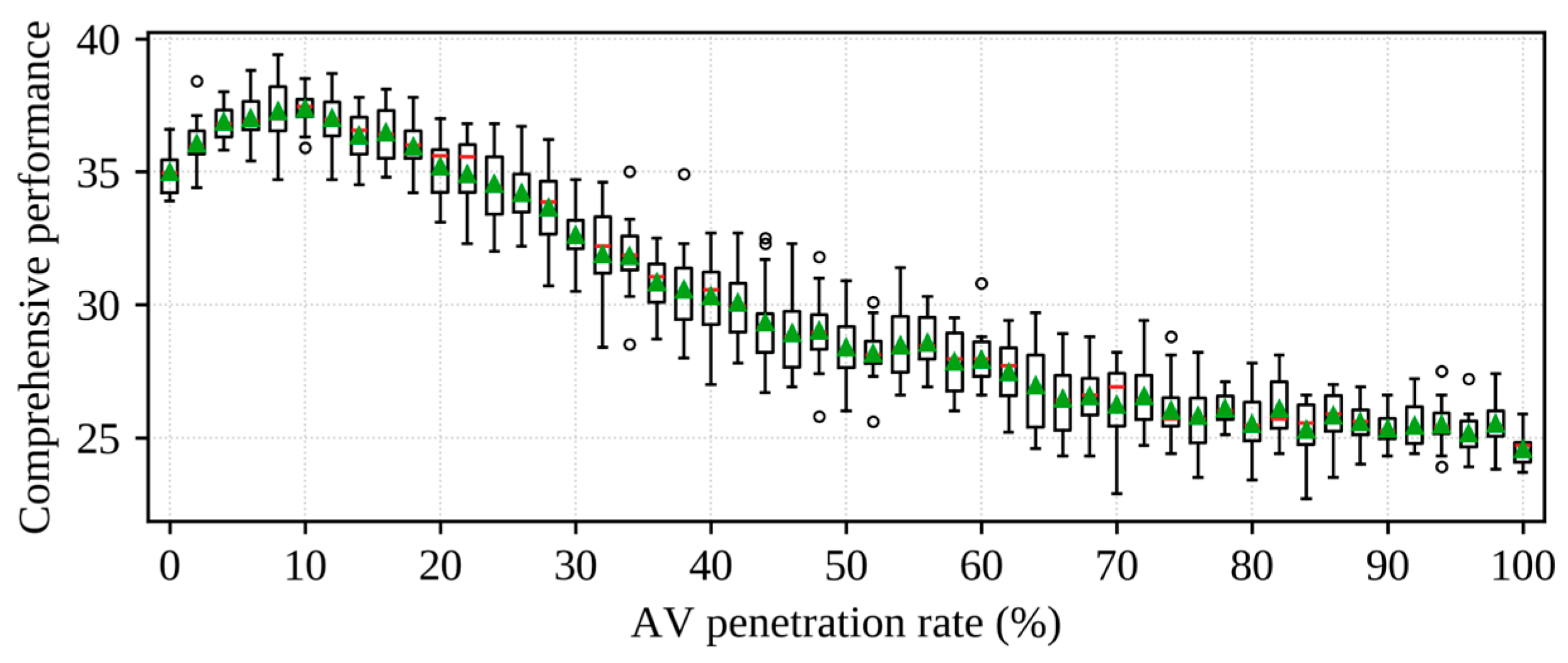
The simulation results verify that the strategy proposed in this paper outperforms the benchmark scheme of the adaptive cruise control system in various test scenarios targeting economy, comfort, and traffic efficiency. Disturbance tests also indicate that perception errors will degrade the vehicle’s economy, comfort, traffic efficiency, and comprehensive performance indicators, yet the strategy maintains a certain degree of robustness. It is noted that, to concentrate on the performance-oriented behaviors of autonomous vehicles at signalized intersections, this paper simplifies the chosen objective, algorithm design, validation scope, and model settings. In future research, we will fully consider the individual characteristics of control strategies and further investigate the influences of weight parameters on diverse decision-making strategies and overall system operational states. Multiple benchmark algorithms will be supplemented, and repeated experimental trials will be implemented. Combined with confidence interval analysis and statistical significance tests, the credibility of the experimental results can be effectively enhanced. Moreover, experiments concerning mixed traffic scenarios and stochastic human driving behaviors will be incorporated to conduct comprehensive validation within intelligent transportation systems, enabling the accurate prediction of vehicle speed fluctuations and improving the precision of decision-making outputs. In addition, various practical traffic influencing factors will be integrated to construct simulation scenarios that better conform to actual traffic operational conditions.

Author Contributions

Conceptualization, X.F. and Y.R.; methodology, P.L. and Y.R.; software, X.F. and Y.R.; validation, T.L. and P.L.; formal analysis, X.F. and P.L.; investigation, Y.R.; resources, Y.R.; data curation, X.F.; writing—original draft preparation, X.F. and T.L.; writing—review and editing, P.L. and Y.R.; visualization, X.F. and P.L.; supervision, P.L. and Y.R.; project administration, T.L.; funding acquisition, P.L. and Y.R. All authors have read and agreed to the published version of the manuscript.

Funding

This study is funded by the Natural Science Foundation of Shandong Province (ZR2024QE314) and the Fundamental Research Funds for the Central Universities (202413022).

Institutional Review Board Statement

Not applicable.

Informed Consent Statement

Not applicable.

Data Availability Statement

The data presented are available on request from the corresponding author.

Conflicts of Interest

The authors declare no conflicts of interest.

References

  1. Wang, B.; Gong, X.; Wang, Y.; Lyu, P.; Liang, S. Coordination for connected and autonomous vehicles at unsignalized intersections: An iterative learning-based collision-free motion planning method. IEEE Internet Things J. 2023, 11, 5439–5454. [Google Scholar]
  2. Agbelie, B.R.D.K.; Roshandeh, A.M. Impacts of signal-related characteristics on crash frequency at urban signalized intersections. J. Transp. Saf. Secur. 2015, 7, 199–207. [Google Scholar]
  3. Wu, L.; Ci, Y.; Chu, J.; Zhang, H. The influence of intersections on fuel consumption in urban arterial road traffic: A single vehicle test in Harbin, China. PLoS ONE 2015, 10, e0137477. [Google Scholar] [CrossRef] [PubMed]
  4. Gao, M.; Nishimura, H. Collision Avoidance Strategy by Utilizing Safety Envelope for Automated Driving System: Hazardous Situation Case. Systems 2026, 14, 89. [Google Scholar] [CrossRef]
  5. Cao, H.; Huang, R. Modeling Individual Risk Decision-Making: A Self-Organization Based Psychological Game Framework [F (T, P, C, R)]. Systems 2026, 14, 60. [Google Scholar] [CrossRef]
  6. Florea, H.; Petrovai, A.; Giosan, I.; Oniga, F.; Varga, R.; Nedevschi, S. Enhanced perception for autonomous driving using semantic and geometric data fusion. Sensors 2022, 22, 5061. [Google Scholar] [CrossRef] [PubMed]
  7. Geng, M.; Chen, Y.; Xia, Y.; Chen, X. Dynamic-learning spatial-temporal Transformer network for vehicular trajectory prediction at urban intersections. Transp. Res. Part C Emerg. Technol. 2023, 156, 104330. [Google Scholar] [CrossRef]
  8. Wu, W.; Deng, X.; Jiang, P.; Wan, S.; Guo, Y. CrossFuser: Multi-modal feature fusion for end-to-end autonomous driving under unseen weather conditions. IEEE Trans. Intell. Transp. Syst. 2023, 24, 14378–14392. [Google Scholar] [CrossRef]
  9. Bouton, M.; Cosgun, A.; Kochenderfer, M.J. Belief State Planning for Autonomously Navigating Urban Intersections. In Proceedings of the 2017 IEEE Intelligent Vehicles Symposium (IV), Los Angeles, CA, USA, 11–14 June 2017; IEEE: New York, NY, USA, 2017; pp. 825–830. [Google Scholar]
  10. Yoon, S.; Lee, D.; Jung, J.; Shim, D.H. Spline-based RRT∗ using piecewise continuous collision-checking algorithm for Car-like vehicles. J. Intell. Robot. Syst. 2018, 90, 537–549. [Google Scholar]
  11. Feng, Y.; Yu, C.; Liu, H.X. Spatiotemporal intersection control in a connected and automated vehicle environment. Transp. Res. Part C Emerg. Technol. 2018, 89, 364–383. [Google Scholar] [CrossRef]
  12. Werling, M.; Kammel, S.; Ziegler, J.; Gröll, L. Optimal trajectories for time-critical street scenarios using discretized terminal manifolds. Int. J. Robot. Res. 2012, 31, 346–359. [Google Scholar]
  13. Qian, L.; Xu, X.; Zeng, Y.; Li, X.; Sun, Z.; Song, H. Synchronous maneuver searching and trajectory planning for autonomous vehicles in dynamic traffic environments. IEEE Intell. Transp. Syst. Mag. 2020, 14, 57–73. [Google Scholar] [CrossRef]
  14. Jin, M.; Qu, M.; Gao, Q.; Huang, Z.; Su, T.; Liang, Z. Advanced trajectory planning and control for autonomous vehicles with quintic polynomials. Sensors 2024, 24, 7928. [Google Scholar] [CrossRef] [PubMed]
  15. Vaskov, S.; Quirynen, R.; Menner, M.; Berntorp, K. Friction-adaptive stochastic nonlinear model predictive control for autonomous vehicles. Veh. Syst. Dyn. 2024, 62, 347–371. [Google Scholar]
  16. Feng, C.; Shen, M.; Wang, Z.; Berntorp, K. Adaptive terminal sliding mode trajectory tracking control for autonomous vehicles considering completely unknown parameters and unknown perturbation conditions. Machines 2024, 12, 237. [Google Scholar] [CrossRef]
  17. Zeng, D.; Zheng, L.; Yang, X.; Li, Y. Uncertainty-aware human-like driving policy learning with deep Bayesian inverse reinforcement learning. Transp. A Transp. Sci. 2025, 21, 2318621. [Google Scholar]
  18. Xu, B.; Ban, X.J.; Bian, Y.; Li, W.; Wang, J.; Li, S.E.; Li, K. Cooperative method of traffic signal optimization and speed control of connected vehicles at isolated intersections. IEEE Trans. Intell. Transp. Syst. 2018, 20, 1390–1403. [Google Scholar] [CrossRef]
  19. Yang, H.; Rakha, H.; Ala, M.V. Eco-cooperative adaptive cruise control at signalized intersections considering queue effects. IEEE Trans. Intell. Transp. Syst. 2016, 18, 1575–1585. [Google Scholar] [CrossRef]
  20. Ubiergo, G.A.; Jin, W.L. Mobility and environment improvement of signalized networks through Vehicle-to-Infrastructure (V2I) communications. Transp. Res. Part C Emerg. Technol. 2016, 68, 70–82. [Google Scholar] [CrossRef]
  21. Abdulhai, B.; Pringle, R.; Karakoulas, G.J. Reinforcement learning for true adaptive traffic signal control. J. Transp. Eng. 2003, 129, 278–285. [Google Scholar] [CrossRef]
  22. Zhao-Meng, C.; Xiao-Ming, L.; Wen-Xiang, W. Optimization method of intersection signal coordinated control based on vehicle actuated model. Math. Probl. Eng. 2015, 2015, 749748. [Google Scholar] [CrossRef]
  23. Xu, B.; Ban, X.J.; Bian, Y.; Wang, J.; Li, K. V2I Based Cooperation Between Traffic Signal and Approaching Automated Vehicles. In Proceedings of the 2017 IEEE Intelligent Vehicles Symposium (IV), Los Angeles, CA, USA, 11–14 June 2017; IEEE: New York, NY, USA, 2017; pp. 1658–1664. [Google Scholar]
  24. Liao, P.; Wang, T.; Tang, T.Q.; Liu, R. Two-stage lane-changing driving strategy based on driving habits and vehicle dynamics for autonomous electric vehicles. IEEE Trans. Intell. Transp. Syst. 2025, 26, 14648–14664. [Google Scholar] [CrossRef]
  25. Liao, P.; Tang, T.Q.; Liu, R.; Huang, H.-J. An eco-driving strategy for electric vehicle based on the powertrain. Appl. Energy 2021, 302, 117583. [Google Scholar] [CrossRef]
  26. Zhou, M.; Yu, Y.; Qu, X. Development of an efficient driving strategy for connected and automated vehicles at signalized intersections: A reinforcement learning approach. IEEE Trans. Intell. Transp. Syst. 2019, 21, 433–443. [Google Scholar] [CrossRef]
Figure 1. Schematic diagram of vehicle–road–cloud integrated traffic system.
Systems 14 00852 g001
Figure 2. Schematic diagram of an autonomous vehicle driving system at signalized intersections.
Systems 14 00852 g002
Figure 3. The longitudinal force diagram of a vehicle.
Systems 14 00852 g003
Figure 4. Schematic diagram of strategy framework.
Systems 14 00852 g004
Figure 5. Sensitivity of trajectories to longitudinal displacement demand.
Systems 14 00852 g005
Figure 6. Sensitivity of trajectories to lateral displacement demand.
Systems 14 00852 g006
Figure 7. Vehicle trajectories under different traffic demands.
Systems 14 00852 g007
Figure 8. Vehicle trajectories under different green ratios.
Systems 14 00852 g008
Figure 9. Vehicle trajectories under different strategy trigger region lengths.
Systems 14 00852 g009
Figure 10. Box plots of comprehensive performance under different AV penetration rates.
Systems 14 00852 g010
Figure 11. Box plots of the influence of lane changing factors on strategy application.
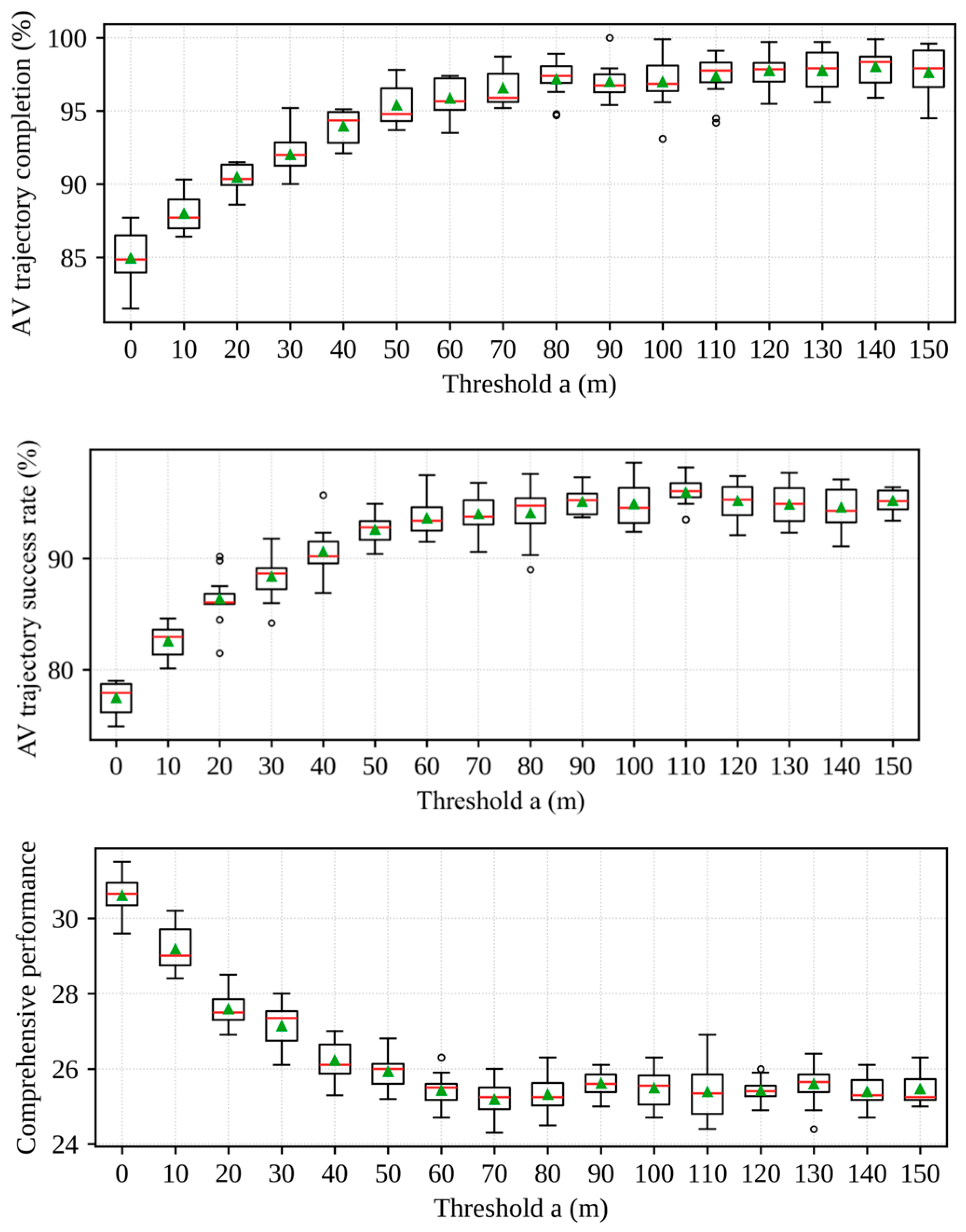
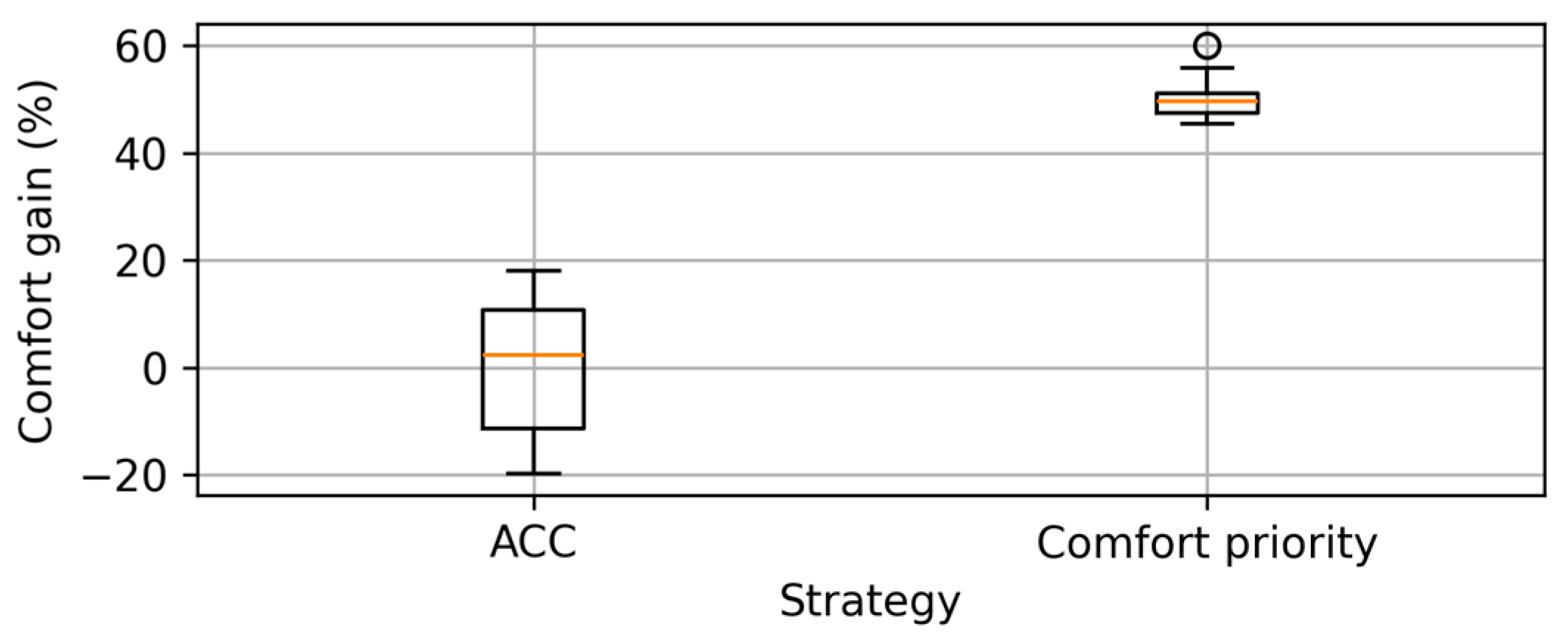
Systems 14 00852 g011
Figure 12. Box plots of comfort performance: comfort-oriented strategy versus ACC strategy.
Systems 14 00852 g012
Figure 13. Box plots of economic performance: proposed strategy versus ACC strategy.
Systems 14 00852 g013
Figure 14. Box plots of efficiency performance: efficiency-oriented strategy versus ACC strategy.
Systems 14 00852 g014
Figure 15. Box plots of the influence of disturbances on strategy application.
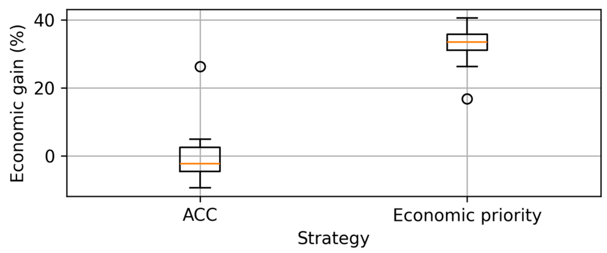
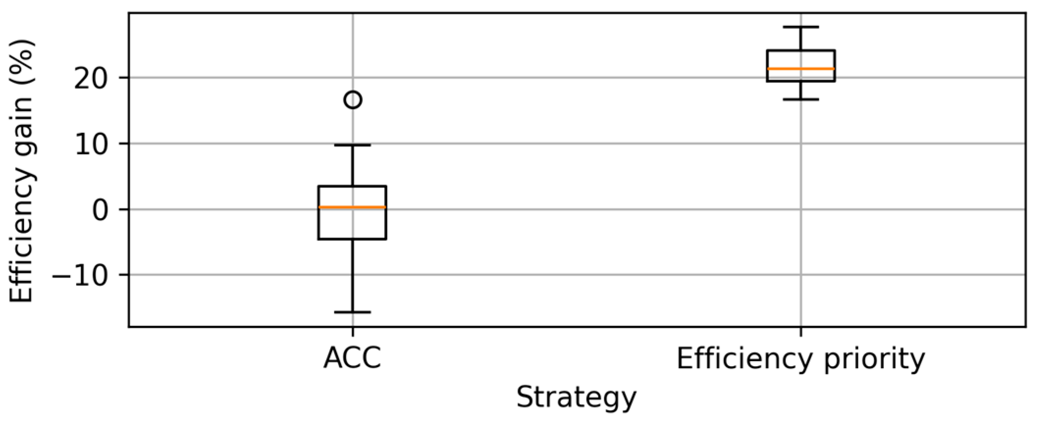
Systems 14 00852 g015
Figure 16. Relative frequency distribution and normal fitting of longitudinal acceleration.
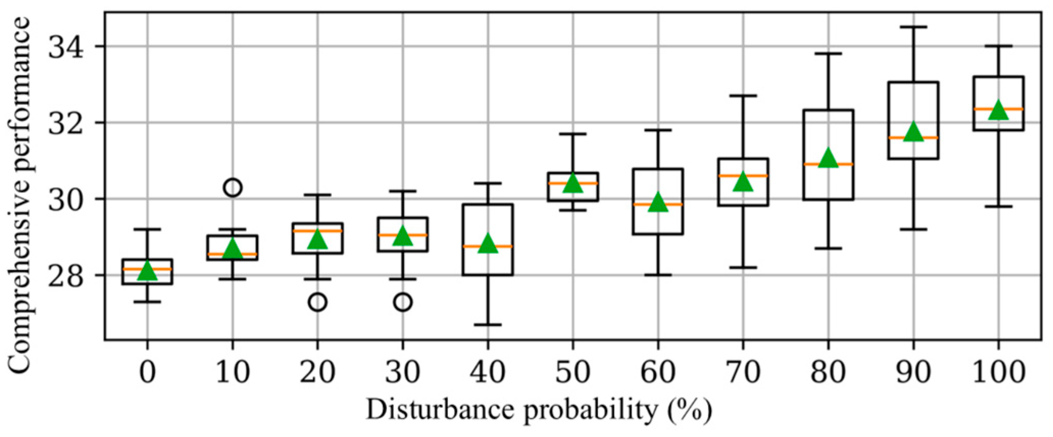
Systems 14 00852 g016
Figure 17. Relative frequency distribution and normal fitting of lateral acceleration.
Systems 14 00852 g017
Table 1. Symbols and definitions used in Equations (6)–(17).
SymbolDefinitionUnit/Index
t i n t Initial planning time s
t s t a Strategy execution duration s
S ( t ) Total longitudinal displacement demand m
d n l o n , e g o ( t i n t + t s t a ) Target longitudinal position at the end of the planning interval m
d n l o n , e g o ( t i n t ) Initial longitudinal position of the ego vehicle m
n l a n Number of remaining lane change actions-
d n l o n , e g o , ( t ) Corrected longitudinal target of the n-th phase m
t n s t a Execution time assigned to the n-th phase s
η s t r Stage allocation coefficient-
t s t r , Total strategy execution time used for phase allocation s
I D s t a Number of transition phases-
d l o n , e g o t Longitudinal displacement of the ego vehicle m
d l a t , e g o t Lateral displacement or current lateral position of the ego vehicle m
a i , b i (i = 0, 1, …, 5)Coefficients of the longitudinal and lateral quintic polynomials-
W Target lateral displacement of the current phase m
D Longitudinal travel distance during lane changing m
v i , j l o n Assumed constant longitudinal speed for candidate trajectory (i,j) m / s
j * ( t ) Index of the target vehicle selected at time t-
d L a n I D s t a s t a , j l o n t Longitudinal position of candidate vehicle j in the target lane m
d d L a n I D s t a s t a , j + 1 l o n ( t ) Longitudinal gap between two adjacent target-lane vehicles m
d L a n I D s t a s t a , j * * l o n t Longitudinal position of the rear-boundary vehicle m
v L a n I D s t a s t a , j * * l o n ( t ) Longitudinal speed of the rear-boundary vehicle m / s
t e x p Desired time headway s
l v e h Vehicle length m
d n l a t , e g o Lateral target position of the ego vehicle in the n-th phase m
d L a n I D s t a s t a , n l o n Lateral position of reference vehicle n in the target lane m
l w Vehicle width m
{ k 1 ,   j + 1 } Candidate vehicle index set considered in the current phase-
Table 2. Simulation parameter settings.
SymbolDefinitionValue/Unit
t Simulation time interval 0.1   s
η s t r Stage time allocation coefficient 0.2
l w Vehicle width 1.7   m
t e x p Time headway 2   s
l v e h Vehicle length 4   m
η 0 Drivetrain efficiency 0.85
W Target lateral displacement 3.5   m
ω j Vehicle performance coefficient, where j 1,2 , 3 [ 1 ,   1 ,   1 ]
a m a x s t o Maximum vehicle deceleration 4   m / s 2
a m a x s t a Maximum vehicle acceleration 3   m / s 2
v 0 Average vehicle speed at entry 10   m / s
d s t o Parking spacing 2   m
Table 3. Performance indicators under different longitudinal displacement demands.
Trajectory TypeLongitudinal Displacement Demand (m)Energy Consumption (KJ/m)Acceleration
Fluctuation
Completion Time (s)
ECO306.6211.5
602.02.83
901.10.864.5
1200.770.366
1500.630.197.5
COM306.8211.6
602.02.83
901.10.864.5
1200.770.366
1500.630.197.5
EFF30442041
6021542
9014253
12011144
1508.89.05
Table 4. Performance indicators under different lateral displacement demands.
Trajectory TypeLateral
Displacement Demand (m)
Energy
Consumption (KJ/m)
Acceleration FluctuationCompletion Time (s)
Economic trajectory3.52.02.83
73.55.33.1
10.55.07.53.2
146.49.33.3
Comfort trajectory3.59.02.473
73.55.33.1
10.58.45.96.4
148.76.06.4
Efficiency trajectory3.521542
722562
10.524602
1426652
Table 5. Strategy performance under different traffic demands.
Traffic Demand (veh/h)Economy (KJ/km)ComfortEfficiency (s)
5000.03610.040235.3
10000.04210.12535.2
20000.04570.044140.1
Table 6. Strategy performance under different green ratios.
Green RatioEconomy (KJ/km)ComfortEfficiency (s)
20%0.01920.027255.3
50%0.05220.18535.3
100%0.05020.1567.4
Table 7. Strategy performance under different strategy trigger region lengths.
Strategy Trigger Region Length (m)Economy (KJ/km)ComfortEfficiency (s)
200.01980.054737.2
500.05220.18535.3
1000.02680.026637.3
Table 8. The 67.5% concentration intervals of longitudinal and lateral acceleration.
DirectionVehicle TypeMean (m·s−2)Std (m·s−2)67.5%
Concentration Interval (m·s−2)
Interval Width (m·s−2)
LongitudinalHV0.0290.919[−0.875, 0.934]1.810
LongitudinalAV0.0170.590[−0.564, 0.597]1.161
LateralHV0.0000.221[−0.218, 0.218]0.436
LateralAV−0.0010.144[−0.142, 0.141]0.283
Table 9. Concentration interval widths and acceleration convergence degrees.
DirectionHV Interval WidthAV Interval WidthWidth
Reduction
Relative
Difference
Actual Narrowing
Rate Relative to HV
Longitudinal1.8101.1610.64855.8%35.8%
Lateral0.4360.2830.15353.9%35.0%
Disclaimer/Publisher’s Note: The statements, opinions and data contained in all publications are solely those of the individual author(s) and contributor(s) and not of MDPI and/or the editor(s). MDPI and/or the editor(s) disclaim responsibility for any injury to people or property resulting from any ideas, methods, instructions or products referred to in the content.