Article

An Explainable Machine Learning Framework Based on XGBoost-SHAP and Multi-Source Geospatial Data: Systematic Analysis of Urban Vitality and Influencing Factors in Changsha

1
School of Architecture and Art, Central South University, Changsha 410083, China
2
School of Humanities and Arts, Hunan International Economics University, Changsha 410205, China
*
Author to whom correspondence should be addressed.
Systems 2026, 14(7), 842; https://doi.org/10.3390/systems14070842
Submission received: 2 June 2026 / Revised: 12 July 2026 / Accepted: 13 July 2026 / Published: 15 July 2026

Abstract

The formation mechanisms of Urban Vitality have been constrained by the limitations of traditional linear driving hypotheses, and the fragmented analysis of subjective and objective factors. Integrating the explainable machine learning model XGBoost-SHAP with multi-source geospatial data, this study constructs a systematic analysis framework at the community scale, comprising 275 community units across five administrative districts in Changsha. It constructs a systematic analysis framework that unifies objective environmental conditions and subjective perceptions—a deliberate departure from the fragmented approaches dominant in previous vitality research. Through this objective-subjective integrated lens, it explores the spatial patterns, non-linear driving mechanisms, and variable interaction effects of Urban Vitality. The XGBoost model achieves a cross-validated R2 of 0.794 and an RMSE of 0.031, ensuring interpretative reliability for exploring non-linear mechanisms. The results indicate that Urban Vitality exhibits a spatial pattern characterized by “high-value aggregation in the core, gradient decay in the periphery, and local fragmentation,” with a significant siphon effect observed in the core area. Partial Dependence Plot (PDP) analysis reveals that the impacts of variables on vitality can be categorized into four patterns: continuous upward, threshold leap, inverted U-shaped, and weak or sample-concentrated. Univariate dependence plots further delineates fine-grained threshold effects, including “threshold triggering, nterval suitability, high-value suppression, and co-occurrence signals.” Furthermore, bivariate interactions reveal four synergistic mechanisms: Building Density must match road network support; Functional Aggregation should synergize with locational value; transportation nodes must integrate with activity-support capacity; and Street View quality and human demand mutually regulate each other. The conclusion asserts that urban stock renewal must transcend the mindset of single-factor maximization and shift towards a precision governance approach of “threshold activation, synergistic matching, and zoning intervention,” thereby providing a quantitative decision-making basis for human-oriented, fine-grained urban regulation.

1. Introduction

Urban Vitality is a crucial indicator of urban livability, economic resilience, and social cohesion, reflecting the aggregation intensity, interaction frequency, and behavioral diversity of human activities within urban spaces [1]. Vibrant urban spaces signify not only bustling streets and lively communities but also embody a city’s sustained attractiveness to talent, capital, and innovation. Enhancing Urban Vitality plays an irreplaceable role in improving the quality of life for residents and fostering sustainable urban development. With the continuous advancement of China’s New Urbanization Strategy [2], the “human-oriented” philosophy of urban development has evolved from a policy slogan into a national strategic initiative. Against this backdrop, scientifically comprehending and precisely stimulating Urban Vitality has emerged as a cutting-edge, interdisciplinary research focus shared by fields such as urban planning, geography, sociology, and public administration.
Since the classical theories of Urban Vitality proposed by scholars such as Jane Jacobs [3] and Montgomery [4], extensive research has confirmed that diverse street functions, mixed land-use patterns, and spatial scales suitable for walking and lingering are crucial environmental conditions for fostering Urban Vitality [5,6]. However, rapid urbanization and disorderly spatial expansion have triggered a series of modern “urban diseases,” including “ghost cities,” urban decay, population outflow, and traffic congestion. Consequently, urban development is shifting from extensive outward expansion to intensive internal renewal [7]. This transition imposes higher demands on spatial governance, necessitating a departure from the traditional mindset dominated by physical construction to seek scientific pathways for precisely identifying, activating, and sustaining spatial vitality in the long term. Otherwise, some urban renewal projects may be reduced to superficial morphological beautification, yielding negative impacts [8] and leading to inefficient public investment or even recurrent spatial decline.
For a long time, built environment theories represented by the 3D [9] and 5D [10] models have dominated Urban Vitality research. These theories have established relatively mature quantitative evaluation systems through dimensions such as functional attributes, architectural morphology, socio-economic indicators, land-use structure, and community characteristics [11,12,13]. With the deepening of the “human-oriented” urban development philosophy and the rise of big data and artificial intelligence technologies, Urban Vitality research is experiencing a significant paradigm shift. Researchers have increasingly recognized that while the objective environment merely provides a spatial carrier for vitality, the subjective perceptions of residents and users (such as sense of security, comfort, and place identity)—and the behavioral choices these perceptions trigger—serve as equally vital intrinsic driving forces for Urban Vitality [14,15,16]. This realization has shifted the research focus from “what is in the space” to “what people perceive,” thereby expanding the theoretical boundaries of human-environment relations. It is worth emphasizing that a growing body of empirical research indicates that the impacts of subjective and objective factors on Urban Vitality are not simple linear superpositions; rather, they exhibit significant non-linear relationships, threshold effects, and complex interactive mechanisms [13,17,18]. For instance, increasing building density within a certain range can promote vitality, but exceeding the threshold may yield negative effects [19]. Similarly, lively and safe streetscapes can amplify the vitality generated by functional mixing [20], whereas a chaotic and unkempt environment can inhibit or even reverse potential vitality. Therefore, accurately identifying key subjective and objective driving factors and deconstructing the underlying mechanisms of the non-linear synergistic interaction between “subjective perception” and the “objective environment” provides a solid evidence-based foundation for high-quality urban renewal and the refined enhancement of spatial vitality.
Reviewing the evolution of Urban Vitality research, early studies primarily relied on statistical and remote sensing data [21]. The studies focused on analyzing urban morphology and functional structures at a macro scale, verifying the positive linear impacts of factors such as population density, land-use mix, and transport accessibility on vitality [22,23]. However, data in this phase suffered from slow update cycles and low spatial resolution. Simple models, such as linear regression, failed to capture complex mechanisms and largely ignored individual perceptions and behavioral choices. With the advancement of the mobile Internet and communication technologies, researchers began to incorporate novel data sources, including social media [24,25,26], Points of Interest (POI) [27,28], Baidu Heatmaps [29,30], and mobile phone signaling data [5,11,31]. For instance, social media texts and images were utilized to mine public emotions and cognitions [32,33,34], while Baidu Heatmaps enabled the real-time capture of dynamic crowd activities [35,36]. Although this phase preliminarily established a connection between the objective environment and subjective perception, the two were typically analyzed in separate models, lacking a systematic deconstruction of their interactive effects. Furthermore, the measurement of subjective perception primarily relied on questionnaire surveys or textual analysis [37,38], making high-resolution, large-scale quantification difficult to achieve.
In recent years, with the rise of explainable machine learning, Urban Vitality research has entered a phase of deep integration. In terms of data measurement, the combination of Street View imagery with deep learning semantic segmentation models (e.g., the SegNet and DeepLab series) [5,17,39,40] has enabled the large-scale quantification of street-level visual environmental features. Researchers can now extract refined indicators from Street View images, such as the green visibility index, sky openness, and building interfaces [16,18,40], thereby breaking the technical bottlenecks of traditional on-site surveys characterized by high costs and limited spatial scopes. Regarding analytical paradigms, algorithms such as Random Forest [41,42], XGBoost [42,43], and LightGBM [5,44] have been widely applied to capture the non-linear relationships between high-dimensional features and Urban Vitality. Assisted by post hoc interpretation tools like Shapley Additive exPlanations (SHAP) [16,29,45,46] and Partial Dependence Plots (PDP) [43], researchers can now unveil marginal effects, threshold intervals, and complex interactive mechanisms among variables [7,47], with the research scale gradually refining from the city as a whole to streets [26], parks [48], waterfronts [49], and transit station areas [50].
However, despite explainable machine learning enhancing model transparency, current studies still suffer from a lack of precise measurement of subjective perceptions. Traditional perception measurement methods (e.g., questionnaire surveys [51] and the semantic differential method [52]) are costly, constrained by limited sample sizes, and possess low spatial resolution. These limitations have long restricted the incorporation of subjective factors into large-scale vitality modeling. Recently, breakthroughs in computer vision and deep learning have offered novel pathways to overcome this bottleneck. The Place Pulse project by the MIT Media Lab, utilizing crowdsourced voting, constructed a human perception dataset covering tens of thousands of Street View images across six dimensions: “Safety, Beautiful, Lively, Wealthy, Boring Depression” Perception [53]. By training Convolutional Neural Networks (CNN) on this dataset, researchers can now predict perception scores for Street View images at any location on a massive scale. This advancement enables subjective perceptions to be quantified and integrated into Urban Vitality driving models [15,16,54], providing robust methodological support for the profound fusion of subjective and objective data.
Despite the significant progress achieved in theoretical perspectives and methodological tools, current research still faces several critical bottlenecks that urgently require breakthroughs. Firstly, there are technical barriers arising from data heterogeneity. Objective environmental data characterize the material attributes of physical space, while subjective perception data reflect individuals’ experiential cognition [16,55]. These two types of data exhibit fundamental differences in their composition, posing substantial obstacles to large-scale cross-scale integration. For instance, multi-source spatial data—such as POIs, Baidu heatmaps, remote sensing imagery, and social media data [43]—differ not only in coordinate systems and spatial scales, but also in data structures (raster vs. vector) and temporal granularities (real-time vs. static). Each of these discrepancies introduces specific integration challenges: coordinate transformation may cause positional errors; scale rescaling (e.g., aggregating point-based POIs to grid cells) inevitably smooths out fine-grained spatial variation; and aligning temporally incompatible datasets often requires coarse-grained averaging, which obscures short-term fluctuations. These preprocessing steps collectively complicate data integration. Secondly, there is an inadequate deconstruction of synergistic interactive effects. Even when explainable machine learning is applied, most analyses still focus predominantly on the driving factors of the objective environment [56], lacking a systematic identification of the complex interaction patterns—such as synergistic enhancement or mutual inhibition—between subjective perceptions and objective environmental variables. Thirdly, there are limitations regarding the static representation of Urban Vitality. The utilized dynamic data primarily rely on cross-sectional data from specific time periods (e.g., POI density [57] or variations in Baidu Heatmaps over a few days [58]). These fail to accurately capture the high-frequency dynamic changes in Urban Vitality across different time periods, such as between weekdays and holidays, resulting in a lack of crucial systemic comparative analysis regarding driving mechanisms across the temporal dimension.
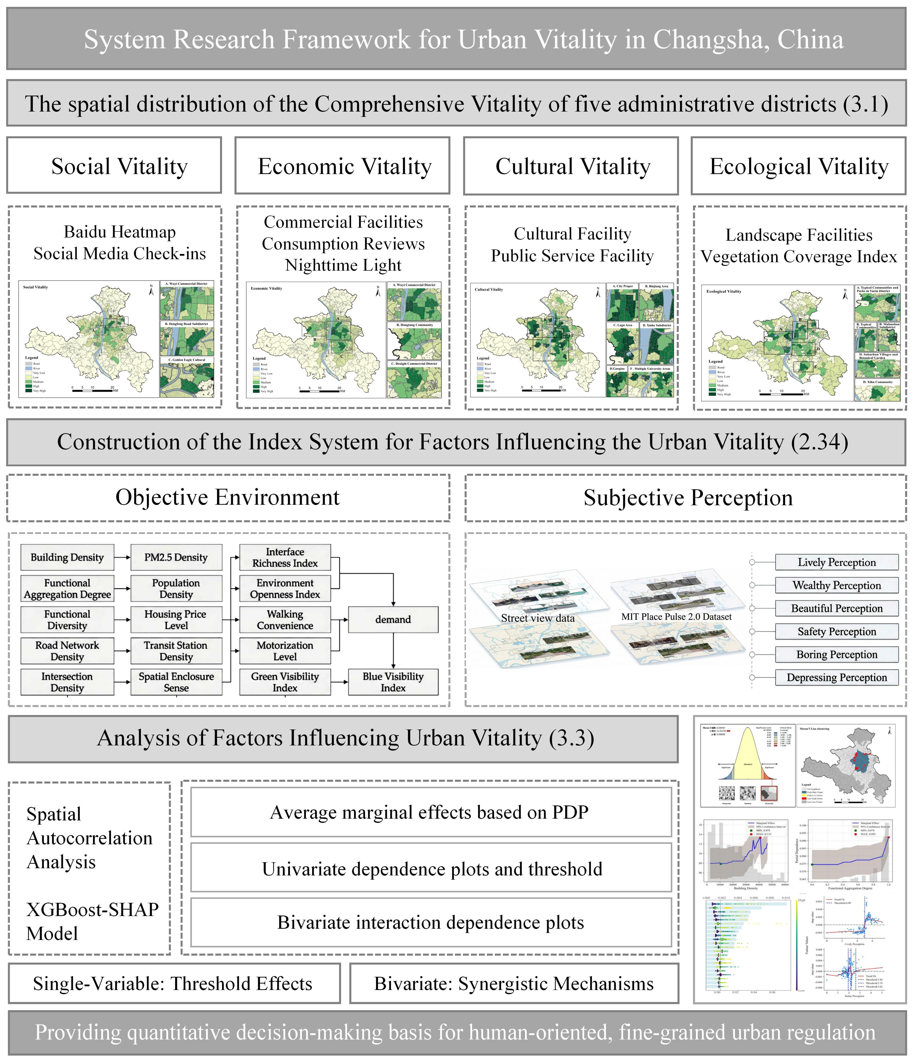
To address the aforementioned research gaps, this study proposes a research framework integrating multi-source geospatial big data and explainable machine learning (Figure 1). Selecting the five administrative districts of Changsha, China, as the empirical case, this research focuses on the dual dimensions of “subjective perception and objective environment” to precisely measure their non-linear driving mechanisms and threshold effects on Urban Vitality. The main innovations of this study are manifested in the following three aspects:
  • Expansion of evaluation dimensions: Constructing a “Subjective-Objective integrated” framework. Current Urban Vitality evaluation systems predominantly focus on objective environment, lacking consideration of micro-scale, human-centric perspective, making it difficult to fully capture the complex dynamic mechanisms of vitality. Building upon previous research [15,16,54], our framework expands upon them by introducing a more comprehensive indicator system with a wider range of variables and dimensions, thereby capturing the multi-layered characteristics of urban space more thoroughly.
  • Exploration in perception quantification: Utilizing deep learning and Street View imagery to break the limitations of traditional subjective evaluations. This study introduces Baidu Street View imagery and performs semantic segmentation to extract micro-visual features. Simultaneously, it integrates the emotional perception dataset provided by MIT Place Pulse 2.0 Dataset to predict emotional labels for the Street View images, successfully quantifying the emotional perception characteristics of urban spaces.
  • Refinement of vitality representation: Introducing multi-source geospatial data to precisely capture dynamic Urban Vitality. Traditional Urban Vitality research mostly relies on static environmental cross-sectional data, which struggles to reflect the high-frequency dynamic changes of human activities. This study incorporates multi-source heterogeneous data—including POIs, Baidu Heatmaps, Street View Image, Social social sensing data (Sina Weibo and Dazhong Dianping)—as representation indicators of spatial vitality. These datasets can reflect the aggregation patterns and preferences of crowds in urban spaces in real-time and with high precision, providing a more reliable empirical basis for unveiling the genuine, dynamic driving mechanisms of Urban Vitality.
Figure 1. System Research Framework Diagram.
Systems 14 00842 g001

2. Materials and Methods

2.1. Research Area

This study selects five administrative districts (Furong, Tianxin, Kaifu, Yuhua, and Yuelu) in Changsha, Hunan Province, China, as the empirical study area (Figure 2), covering a total area of approximately 1204.89 km2. This study selects the five districts of Furong, Tianxin, Yuelu, Kaifu, and Yuhua as research subjects, which serve as the core functional areas for politics, economy, science and technology innovation, and culture in Changsha. Furong is the financial and commercial center, Tianxin the administrative and cultural core, Yuelu the zone for science and education innovation, Kaifu the hub for cultural creativity and logistics, and Yuhua the base for commerce, trade, and advanced manufacturing. They differ markedly in development intensity, industrial structure, and spatial morphology, thus providing ideal samples for investigating the differentiation mechanisms of Urban Vitality across different types of urban districts.

2.2. Data Sources and Processing

2.2.1. Multi-Dimensional Urban Vitality Dataset

To comprehensively characterize Urban Vitality, this study constructs a measurement indicator system comprising four dimensions: economic, social, cultural, and ecological (Table 1).
Social Vitality is represented by multi-period heat maps from Baidu Maps Huiyan and social media check-ins. On the one hand, it based on the principle of stratified sampling, Baidu Heatmap data for 24 days across the 12 months of 2025 within the five administrative districts of Changsha were selected. Specifically, one weekday and one weekend day were selected for each month, explicitly excluding days with extreme weather conditions (e.g., high temperatures, rainstorms) and special holidays (e.g., Spring Festival, National Day, and Labor Day), ultimately yielding 576 sets of heatmap data. The raw data were subsequently transformed into the WGS-84 coordinate system and clipped to the study area to map the point-based heat values onto regular analytical grids. Following this, the mean values across all time points within a 24 h period were calculated to derive the average crowd vitality index. On the other hand, the selected social media check-in data were sourced from Sina Weibo, serving as a spatial mapping of online digital traffic. A Python web crawler was utilized to extract data—including text content, posting time, user ID, comment counts, and like counts—generated between 1 January 2025, and 31 December 2025. After removing duplicate entries based on post IDs, filtering out posts with empty content or missing timestamps, and excluding data points located outside the five administrative districts of Changsha, a total of 272,426 valid records were retained. To ensure data reliability, 200 samples were randomly selected and manually cross-checked against the original web pages, yielding a perfect consistency match.
Economic Vitality is composed of commercial service facilities, consumption reviews, and nighttime light intensity. Data for commercial service facilities were sourced from Amap. A Python web crawler was utilized to extract POIs data within community units—including catering, shopping, entertainment, and accommodation—which contained information such as longitude, latitude, name, address, category, and administrative district. To ensure data reliability and analytical reproducibility, strict cleaning rules were applied during preprocessing: (1) duplicate records with identical names and geographical coordinates were eliminated; (2) invalid data containing missing coordinates were removed; and (3) locations falling outside the official administrative vector boundaries of the five central urban districts were clipped and excluded. Following this cleaning procedure, the final validated dataset comprised 136,201 commercial service facilities. Data on consumption activity were derived from Dazhong Dianping, obtained by systematically crawling the Changsha index and iterating through commercial classification URLs via custom Python scripts. After removing entries lacking valid data for stars, ratings, prices, or reviews, and excluding locations with incomplete store information or those situated outside the five administrative districts of Changsha, a total of 117,099 valid records were ultimately retained. Additionally, nighttime light intensity data utilized the annual composite data provided by the National Earth System Science Data Center. Its annual temporal scale effectively smooths out short-term fluctuations, thereby reflecting the regional economic activity intensity level more stably.
Cultural Vitality is composed of cultural facilities and public service facilities. It includes the number of POIs for museums, libraries, art galleries, theaters, cultural centers, exhibition halls, media institutions, bookstores, and cultural and creative shops within community units. The data sources and cleaning rules are identical to those for the economic vitality POIs mentioned above, ultimately yielding 22,788 valid records. Public service facilities encompass the number of POIs for schools, research institutions, training agencies, sports and leisure venues, and medical and healthcare centers within community units, ultimately yielding 32,372 valid records.
Ecological Vitality comprises the POIs of landscape facilities and the vegetation coverage index. The data sources and cleaning rules for these POIs are identical to those mentioned above, resulting in 1765 valid records. The vegetation coverage index is defined as the average Normalized Difference Vegetation Index (NDVI) within each community units. The NDVI data, which reflects vegetation coverage and health, was sourced from the NASA Earthdata Search platform to evaluate urban Ecological Vitality on a micro scale.
To eliminate dimensional differences and ensure comparability among these multi-source geospatial datasets, all the aforementioned datasets characterizing Urban Vitality were normalized within the community units grids to a dimensionless scale of [0, 1], thereby enabling a consistent evaluation of their relative distribution patterns.

2.2.2. Street View Image Dataset

Street View imagery is a crucial data source for advanced urban analysis, providing users with a realistic visual representation of the urban physical environment [40]. In this study, customized Python scripts were deployed to systematically interface with the Baidu Street View Static Image API, capturing spatial data across the five primary administrative districts of Changsha. Adopting rigorous methodological precedents, virtual sampling coordinates were generated at 50 m increments along the centerlines of the urban road network. At each node, omnidirectional streetscape features were captured by extracting images from four orthogonal headings (0°, 90°, 180°, 270°), ensuring a comprehensive 360-degree panoramic coverage. This raw retrieval process yielded an initial repository of 116,747 static panoramas featuring a high resolution of 2048 × 1024 pixels. To insulate the dataset from anomalies such as seasonal bias or irregular traffic dynamics, a strict multi-tier filtration pipeline was implemented; images recorded during rush hours, national holidays, adverse weather events, or transient road blocks were systematically purged. Furthermore, to optimize data integrity, we discarded repetitive, heavily obstructed, unfocused, or poorly illuminated nocturnal frames, culminating in a refined, temporally balanced dataset of 83,017 high-quality images. Computer vision analysis was subsequently executed using the Mask2Former semantic segmentation architecture pre-trained on the comprehensive ADE20K dataset, which enables dense pixel-level classification across diverse urban components including building envelopes, sky view factors, pavement networks, flora, and transit vehicles. Drawing on previous research [12,17], seven key influential indicators were extracted: Spatial Enclosure Sense, Interface Richness Index, Environment Openness Index, Walking Convenience, Motorization Level, Green Visibility Index, and Blue Visibility Index.

2.2.3. MIT Place Pulse 2.0 Dataset

The MIT Place Pulse 2.0 dataset [17,23,63] was created by the MIT Urban Studies Lab, using Street View images to systematically measure and evaluate the perceived characteristics of urban environments. The dataset was collected through an online platform, where participants rated Street View images across six dimensions: Safety, Lively, Wealthy, Beautiful, Boring, and Depressing [64]. Adopted a statistical method analogous to the concept of “strength of schedule” in sports competitions to compute the perceptual scores for each dimension, with scores ranging from 0 to 10. Finally, this study applied the trained Vision Transformer Base (ViT-B) model to street-level imagery from five administrative districts of Changsha, thereby obtaining perceptual indicators for each dimension. To calculate perceptual scores, we define the win (Wi,u) and loss (Li,u) frequencies for image i on attribute u as follows:
W i , u = w i , u w i , u + l i , u + t i , u
L i , u = l i , u w i , u + l i , u + t i , u
In the formula, w i , u ,   l i , u , t i , u denote the win, loss, and tie counts for image i in pairwise comparisons. Consequently, the perceptual rating score ( Q i , u ) for imagei regarding indicator u is defined as:
Q i , u = 10 3 W i , u + 1 n i w k 1 = 1 n i w W k 1 , u 1 n i l k 2 = 1 n i l L k 2 , u + 1
In the formula, n i w and n i l denote the total number of images that image i won and lost against, respectively. The score Q i , u incorporates the rankings of these compared images. Without loss of generality, the perceptual score is rescaled to a [0, 10] range by adding an offset of 1 and applying a multiplier of 10 / 3 to bound the minimum and maximum scores.
To assess the model’s transferability to the Chinese context, we validated the MIT-trained visual model using manually scored Street View images from Changsha’s five administrative districts. We randomly selected 1000 street-view images across the study area for this validation. Fifty local volunteers (gender-balanced, aged 20–60, with in-depth local knowledge) rated images against the six SVI indicators on a 1–10 scale. After comparison, the manual scores closely matched the model-generated scores, with a Pearson correlation coefficient of r = 0.81 (p < 0.001), confirming that the model performs robustly in the study area, thereby supporting its applicability in the present research.

2.2.4. The Other Basic Dataset

The other basic data for this study mainly include Building Density, Road Network Density, Intersection Density, PM2.5 Density, Housing Price Level, and Transit Station Density. We extracted the Road Network data of the five administrative districts of Changsha for 2025 from OpenStreetMap and combined them to construct the boundaries of community units, establishing spatial topological relationships to form a standardized road network dataset. Building vector data were captured to represent the spatial volume for 2025. For environmental and socioeconomic baselines, annual average PM2.5 concentration raster data for 2024 were sourced from the global PM2.5 remote sensing inversion dataset published by the Atmospheric Composition Analysis Group. Second-hand housing price data for 2024 were acquired using Python web crawler technology from the listing information on the Anjuke platform to reflect regional economic levels and residential value disparities. Transit node data for 2025 were obtained from the Amap Open Platform, extracting POIs for bus and subway stations to characterize public transportation service supply capacity and accessibility.
To ensure comparability and reliability across these heterogeneous multi-source datasets, this study conducted a unified spatio-temporal registration and strict quality control workflow before indicator calculation and model construction. Because the data differed in format, spatial resolution, temporal coverage, and acquisition mechanism, all records were transformed into a unified spatial reference framework and aggregated to community units. For spatial registration, vector datasets—including POIs, social media check-ins, consumption-review points, road networks, transit stations, housing price, and street-view sampling points—were checked for coordinate completeness and validity, and records with missing, duplicated, invalid, or abnormal coordinates were systematically removed. Valid vector data were transformed to the WGS-84 coordinate reference system, clipped to the five central districts of Changsha, and examined through spatial overlay checks to reduce coordinate and geocoding errors.
Within this unified framework, point and line vectors (including POIs, check-ins, transit stations, and housing price) were summarized by count, density, or mean value at the community-unit scale. Specifically, Road Network Density was calculated based on the total length of roads within a unit grid, while Intersection Density and Transit Station Density were calculated by the number of road intersection nodes or transit stations per unit area. Building density, alongside street-view visual and perceptual indicators, was similarly calculated for each community unit grid. For raster datasets, including PM2.5 concentration, NDVI (derived from Landsat 8 OLI and Landsat 9 OLI-2 surface reflectance imagery), and nighttime light intensity, layers were checked for spatial coverage, resolution, and NoData values, then resampled, aligned, and extracted as mean values via zonal statistics. Temporally, 2025 served as the reference baseline year, while the 2024 PM2.5 and housing price data were treated as stable background variables. Although this introduces a certain degree of temporal mismatch, the interannual average changes for both variables between 2024 and 2025 were verified to be within 1%, suggesting that the temporal difference was minor and unlikely to substantially influence the cross-sectional community-level analysis, though the associated uncertainty is acknowledged. Finally, web-crawled records along with street-view images were cleaned and verified, and normalized to a scale of [0, 1] for comprehensive Urban vitality assessment and XGBoost-SHAP modeling.

2.3. Research Methods

2.3.1. Construction of Urban Vitality Indicator System

To maintain consistency in measuring vitality across various dimensions, we performed normalization on social, economic, cultural, and ecological vitality (Equation (4)), and subsequently applied the entropy weight method to determine the weight of each dimension. Finally, these values were weighted and aggregated to derive the comprehensive Urban Vitality index for each community units [29]. Serving as the dependent variable in subsequent models, this index can objectively and comprehensively characterize the level of Urban Vitality at the neighborhood scale. The specific process is as follows:
Indicator normalization:
X = X X m i n X m a x X m i n
In the formula, X′ represents the normalized value of each evaluation unit; X is the original value; Xmax and Xmin denote the minimum and maximum values across all evaluation units, respectively. After normalization, all indicator values are uniformly transformed into the [0, 1] interval, thereby enhancing the comparability among different indicators.
Calculating the weights of the indicators using the entropy weight method:
P i j = X i j i = 1 m X i j
Calculating the information entropy:
e j = k i = 1 m P i j ln P i j
In the formula, e j represents the information entropy of the j-th indicator; P i j represents the proportion of the i-th evaluation unit under the j-th indicator; k is the normalization coefficient used to ensure that the information entropy value falls within the [0, 1] interval; and m denotes the total number of evaluation units. When P i j = 0, it is generally defined that P i j ln P i j = 0 to ensure the rationality of the calculation process. A larger e j information entropy value indicates a smaller variance for that indicator across different evaluation units, meaning it provides less effective information. Conversely, a smaller e j information entropy value indicates a more significant variance for the indicator, reflecting a stronger capacity to distinguish the evaluation results.
Calculating the difference coefficient:
g j = 1 e j
In the formula, g j represents the difference coefficient of the j indicator, also known as the information utility value; e j represents the information entropy of the j-th indicator. The difference coefficient reflects the amount of effective information contained within the indicator. A larger g j indicates a higher degree of dispersion for that indicator across the evaluation units, thus signifying a greater contribution to the comprehensive evaluation; conversely, a smaller value implies a weaker information contribution from that indicator.
Calculating the weights of the indicators:
w j = g j j = 1 n g j
In the formula, w j represents the weight of the j-th indicator; g j represents the difference coefficient of the j-th indicator; n denotes the total number of indicators; and j serves as the summation index. This formula demonstrates the normalization of the difference coefficients across all indicators, ensuring that the sum of all indicator weights equals 1.
Normalizing the weight vector:
j = 1 n w j = 1
After weight normalization, the indicator weights possess additivity and can be used for the subsequent calculation of the comprehensive evaluation index.
Calculating the comprehensive vitality value through weighted summation:
S = j = 1 n w j X j
In the formula, S represents the comprehensive vitality value; X j represents the normalized value of the j -th indicator; and w j represents the weight of the j -th indicator.
Through the aforementioned method, Weibo activity was found to account for the highest weight proportion of 0.334. To verify the methodological robustness of this index framework, we conducted a weighting sensitivity analysis indicating that the entropy-weighted urban vitality was strongly correlated with the dimension-balanced equal-weighted model, yielding Spearman and Pearson correlation coefficients of 0.937 and 0.953, respectively. The comparison of Urban Vitality values further revealed that 68.73% of the community units were assigned to the exact same vitality class, with 98.55% of total units exhibiting a spatial tier discrepancy of no more than one class, suggesting that the primary spatial patterns of Urban Vitality not be solely dictated by the high entropy weight of Weibo activity.

2.3.2. Spatial Autocorrelation Analysis Method

Spatial dependency and clustering tendencies of comprehensive urban vitality were evaluated utilizing spatial autocorrelation techniques, encompassing both global and local Moran’s I statistics. To mathematically formulate these geographic relationships, a spatial weight matrix was configured based on the first-order Queen contiguity criterion. This configuration aligns with established methodological conventions for regular grid structures, providing a robust framework for capturing micro-scale spatial dependencies within the grid-based analytical matrix.
Specifically, the Global Moran’s I index was calculated to diagnose the overarching spatial distribution archetype (whether clustered, dispersed, or random) of the Urban Vitality Index across the study area, formulated as follows:
I = n i = 1 n   j = 1 n   w i j x i x ¯ x j x ¯ S 0 i = 1 n   x i x ¯ 2
To further reveal localized spatial heterogeneity and delineate the precise geography of cold spots and hot spots, the Local Moran’s I, commonly operationalized as the Local Indicators of Spatial Association (LISA), was deployed. By generating LISA cluster maps, this step pinpoints spatial aggregation (High-High and Low-Low clusters) alongside spatial anomalies (High-Low and Low-High outliers), thereby illuminating the structural associations and interface dynamics between dominant core nuclei and peripheral zones. The calculation formula is as follows:
I i = x i x ¯ S 2 j = 1 n   w i j x j x ¯
In the formula, n is the total number of evaluation units; xi and xj represent the Urban Vitality Index for units i and j; x ¯ is the mean value; wij denotes the spatial weight matrix. The value of I ranges from −1 to 1, where a significantly positive outcome confirms spatial concentration among adjacent units, while a significantly negative outcome reveals spatial divergence.

2.3.3. XGBoost-SHAP Model

Extreme Gradient Boosting (XGBoost) is a powerful machine learning algorithm for classification and regression [42,43]. During the model training phase, a total of 275 community units samples were randomly divided into a training set (80%) and a test set (20%) at a ratio of 8:2. To achieve optimal model generalization and prevent overfitting, hyperparameter tuning was performed using Bayesian optimization combined with 5-fold cross-validation, aiming to automatically search for the optimal hyperparameter combination based on cross-validation performance. Compared with grid search, Bayesian optimization can approximate the optimal solution more efficiently in a large parameter space, making it particularly suitable for the joint optimization of continuous parameters such as learning rate, regularization terms, and sampling rate. The specific search space and final selected values are as follows (Table 2).
From the final parameters, the model adopts a combination of learning-rate= 0.0329, max-depth = 3, and n-estimators = 108, indicating that the model primarily uses shallow trees and a moderate number of trees, thereby avoiding excessive complexity in any single tree. The values colsample_bytree = 0.1507 and subsample= 0.1928 suggest that only a small proportion of variables and samples are drawn in each training round, which helps improve robustness and reduce the risk of overfitting. The low values of reg-lambda and gamma indicate that, given the current sampling constraints and tree depth control, the model is already able to maintain good generalization ability. To explain the prediction mechanism of the above XGBoost model at the community units scale, this study further employs the SHAP method to conduct a systematic feature attribution analysis. The SHAP algorithm quantifies the contribution of each predictor to the final outcome by outputting rank-ordered SHAP value [45,46]. This study employs the TreeSHAP polynomial-time algorithm, which tracks the proportion of paths for feature subsets reaching the terminal nodes of decision trees. The approach significantly reduces computational complexity while ensuring the consistency and accuracy of local explanations. The calculation formula is as follows:
ϕ i f , x = S F \ { i } S ! F S 1 ! F ! f x S { i } f x S
In the formula, F represents the set of all features; S is a subset of features, represents a subset of features that does not include feature i; f(S) is the model’s prediction result based on the feature subset S; f S { i } is the prediction result when feature x i is added to the subset S; and S ! F S 1 ! F ! is the weighting coefficient, which measures the probability of different permutations and combinations to ensure absolute fairness in the distribution of marginal contributions.

2.3.4. Influencing Factor Selection

To comprehensively investigate the Influencing Factors of Urban Vitality in the five districts of Changsha, this study constructs a comprehensive measurement system comprising 22 indicators, following the dual logic of subjective perception and objective physical attributes (Table 3).

3. Result Analysis

3.1. Features of Urban Vitality Distribution

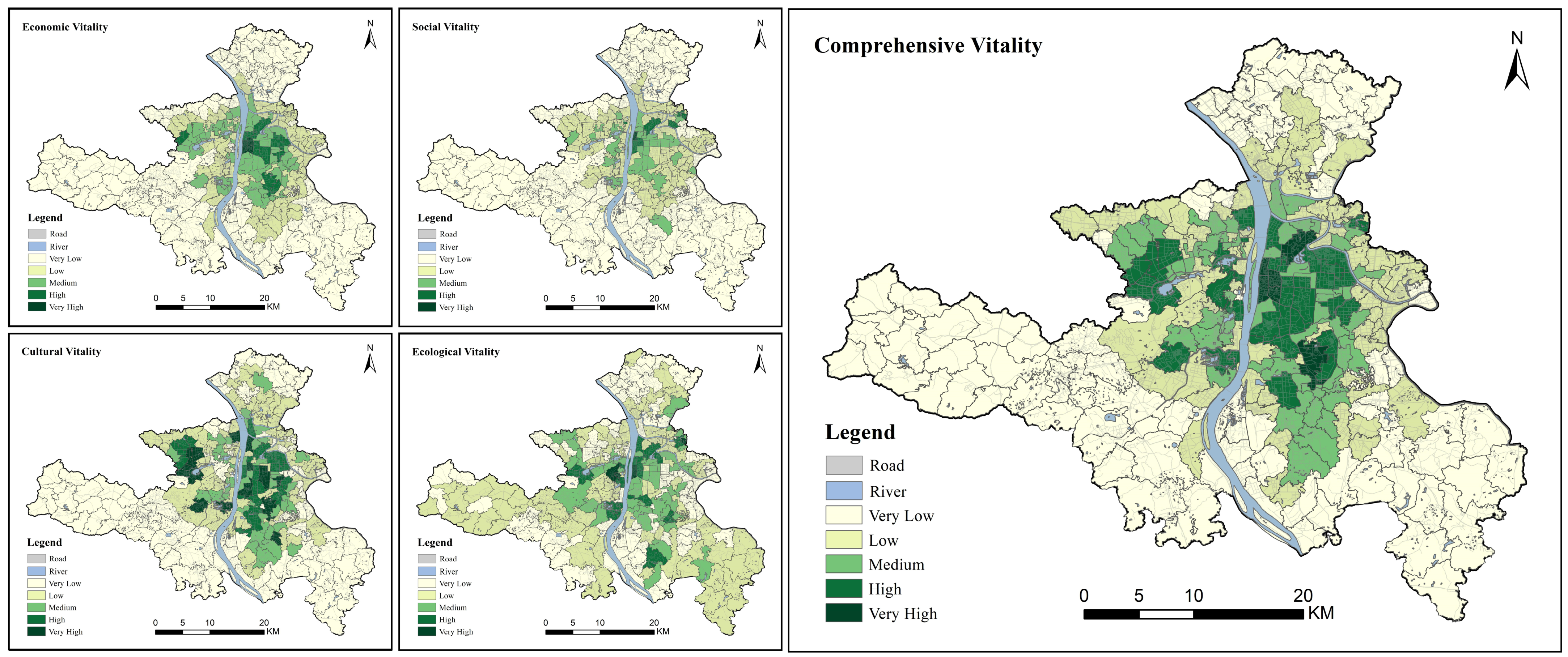
The Urban Vitality in five administrative districts of Changsha presents a spatial pattern characterized by “high-value aggregation in the core, gradient decline toward the periphery, and multiple characteristic scattered points”. Social, Economic, Cultural, and Ecological Vitality are highly coupled in the core business districts, but significantly differentiated in peripheral and nodal areas. The spatial distribution of the Comprehensive Vitality (Using the Jenks natural breaks method, with class breaks of 0.0409, 0.0906, 0.1555, 0.2728, 0.6327) is illustrated in Figure 3.

3.1.1. Social Vitality Distribution Features

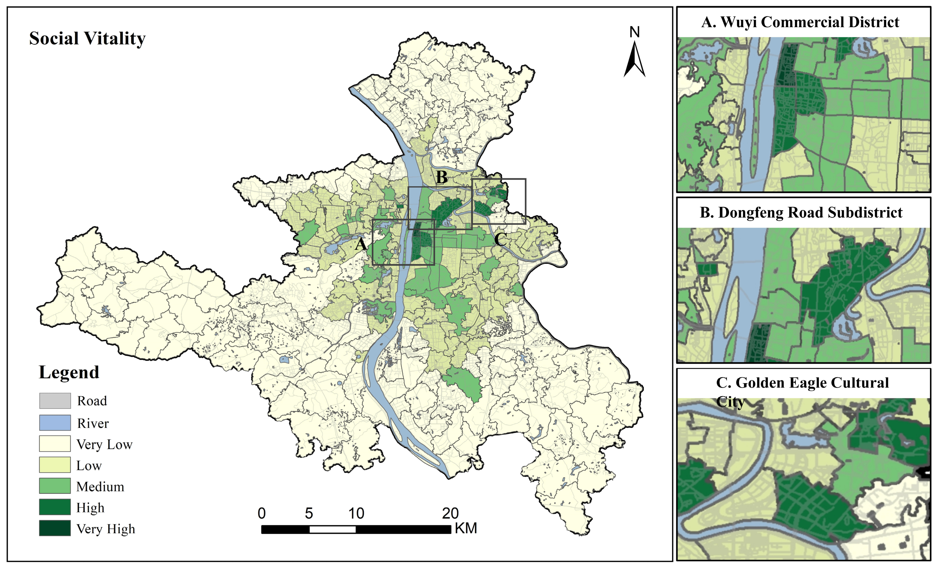
The Social Vitality in the five administrative districts of Changsha presents a spatial pattern characterized by “high-value aggregation in the core and scattered hotspots on the periphery” (Figure 4, Using the Jenks natural breaks method, with class breaks of 0.0094, 0.0267 0.0708, 0.1739, 0.3685).
Class A areas—comprising key urban subdistricts such as Tongtai Street, Pozi Street, and Dingwangtai Stree—constitute the core zone of Social Vitality. Encompassing iconic landmarks like Wuyi Square, the Pedestrian Street, and IFS, these areas experience massive, round-the-clock pedestrian flows and consistently rank as high-heat zones, reflecting exceptional population density and social engagement. This high-activity wave extends to Class B areas like Dongfeng Road Street, which represent sub-high vitality zones primarily driven by cultural and tourism anchors including the Hunan Museum and Martyrs’ Park. Meanwhile, Class C areas, which include Window of the World, the Hunan Broadcasting and Television Center, and Zhaoyang Community, exhibit distinct “patchy peak” characteristics. Among them, the tourism and media hubs of Window of the World and the Broadcasting Center experience sudden surges in popularity during major events but face significant daily fluctuations, whereas Zhaoyang Community maintains a steady baseline of business and travel traffic supported by the Changsha Railway Station district and the Electronics Technology Street.
Figure 3. Spatial distribution map of Comprehensive Vitality.
Systems 14 00842 g003
Figure 4. Spatial distribution map of Social Vitality.
Systems 14 00842 g004

3.1.2. Economic Vitality Distribution Features

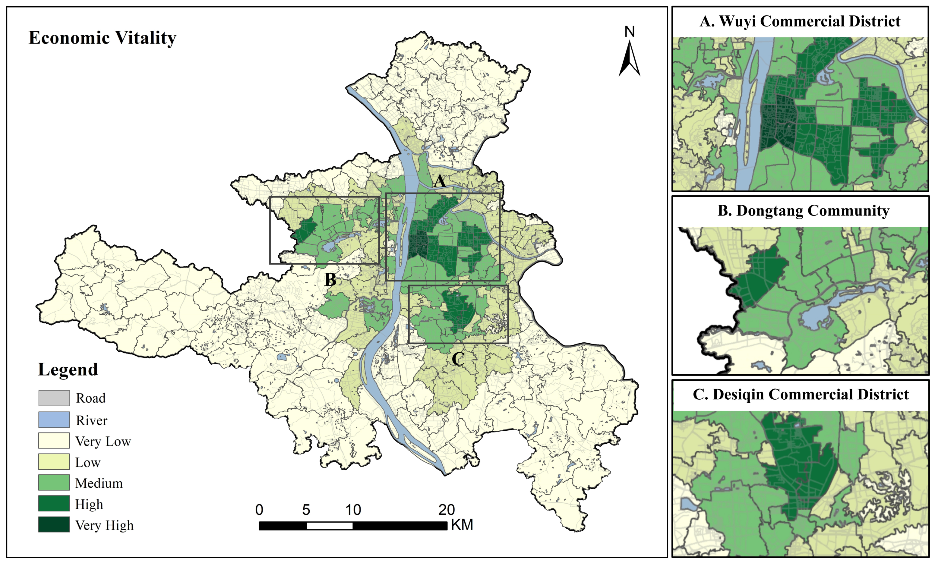
The Economic Vitality of Changsha’s five administrative districts exhibits “multi-centric aggregation and gradient distribution” spatial pattern, structured into three distinct tiers. Class A areas—comprising core subdistricts and nodes such as Pozi Street, Dingwangtai, Chengnan Road, Tongtai Street, Wangluyuan, Qingshuitang, Dongfeng Road, Wenyi Road, Houjiatang, Zuojiatang, Huoxing, Hehuayuan, Dongtundu, Gaoqiao Village, and Sanfenchan—constitute the primary growth poles; they demonstrate a highly synergetic development of commercial supply, consumer behavior, and the nighttime economy. Class B areas, centered on the Dongtang commercial hub, serve as well-established nodes that sustain high consumer foot traffic and commercial clustering by leveraging metro interchange advantages and major retail complexes like Dongtang Department Store and Friendship Mall. Meanwhile, Class C areas (such as Hongxing and Lianhu) anchor the southern urban sub-center, where the Hongxing Global Agricultural Wholesale Center, Desiqin City Plaza, and business clusters around the provincial government drive rapidly emerging modern trade, making this tier a vital economic engine for southern Changsha (Figure 5, Using the Jenks natural breaks method, with class breaks of 0.0152, 0.0367, 0.0677, 0.1374, 0.2925).

3.1.3. Cultural Vitality Distribution Features

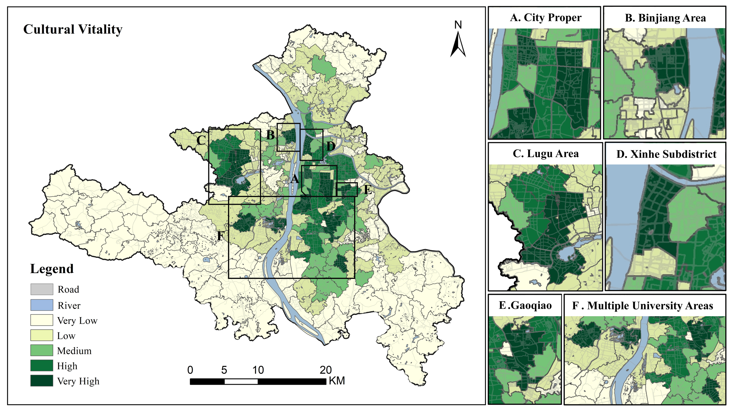
The Cultural Vitality of Changsha exhibits a spatial pattern defined by “core lineage aggregation, new-town cultural integration, and distinctive programmatic nodes.” Class A areas—encompassing Dingwangtai, Chaoyang, and Zuojiatang streets—anchor the historic core of urban culture. Dingwangtai stands as a bastion of historical heritage and public reading, hosting landmarks like the Hunan Provincial Library, the Changsha Bamboo Slips Museum, and the Dingwangtai Book Market. In contrast, Chaoyang leverages its proximity to the Changsha Railway Station, the electronics market, and local theaters to fuse digital subcultures with urban pop culture, while Zuojiatang blends grassroots community identity with modern consumer trends through community cultural centers and industrial heritage adaptive reuse projects (Figure 6, Using the Jenks natural breaks method, with class breaks of 0.0135, 0.0344, 0.0587, 0.0854, 0.1719).
Moving outward, Class B areas within the Binjiang New District balance public services with cultural commerce, anchored by the iconic “Three Museums and One Hall” civic complex (comprising the Changsha Museum, Library, Planning Exhibition Hall, and Concert Hall) alongside riverside commercial hubs like Yuren Wharf. Class C areas, typified by the Lugu High-Tech Zone, feature an “industry-innovation culture” driven by tech professionals through maker salons and informal networks, compensating for a lack of large-scale public infrastructure with enterprise-supported recreation hubs. Nearer the waterfront, Class D areas along Xinhe Street blend sacred and civic spaces, where religious heritage sites like Kaifu Temple and the Changsha Christian Church coexist with the public leisure functions of the riverside scenic belt. Meanwhile, Class E areas, centered around the Gaoqiao Grand Market, manifest a trade-driven folk culture where vitality thrives through market festivals, exhibitions, and trade promotions rather than traditional institutional facilities. Finally, Class F areas form the city’s creative and academic epicenter; encompassing major institutions like Central South University, Hunan University, and Hunan Normal University, this tier integrates landmarks like the historic Yuelu Academy and Houhu Art Park into a dynamic ecosystem of youth-led creative culture, art exhibitions, and nighttime cultural consumption.

3.1.4. Ecological Vitality Distribution Features

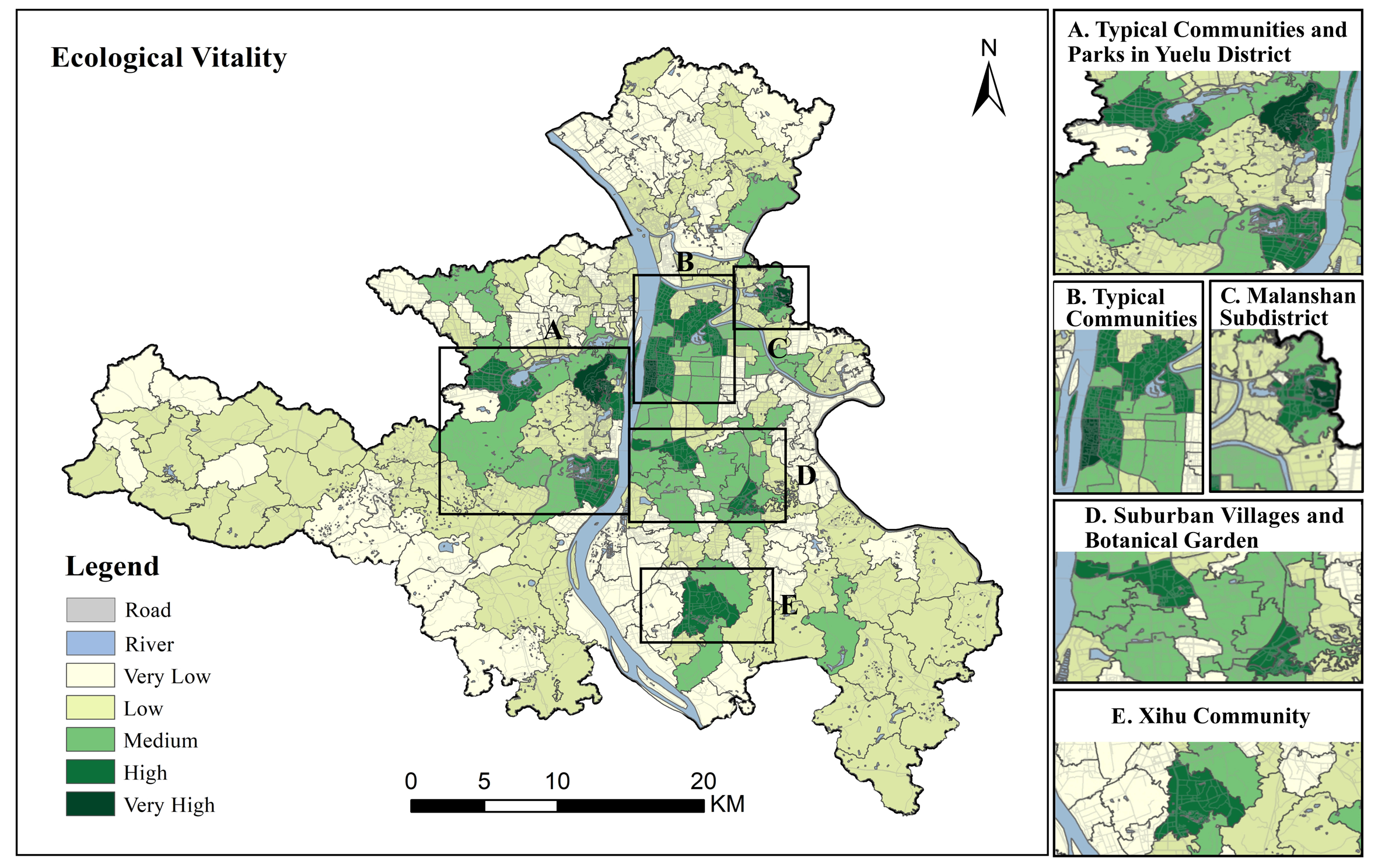
The Ecological Vitality of Changsha exhibits a spatial framework defined by “one core, two belts, and multiple embedded nodes.” Class A areas—comprising Yuelu District Park, the Tianma and Runlong communities, alongside Yanghu and Lianshan villages—constitute the city’s primary ecological core. This zone provides a robust green foundation, highlighted by Yuelu Mountain’s forest coverage exceeding 95% and the Yanghu Wetland’s negative oxygen ion concentration, which reaches six times the urban average. Extending from this core, Class B areas (including Pozi Street, Tongtai Street, Wangluyuan, Dingwangtai, Chengnan Road, Xinhe, Dongfeng Road, Xianghu, and the Orange Isle Community) leverage the Xiangjiang River waterfront to form a continuous riparian ecological corridor. Within this corridor, Orange Isle serves as a pivotal axis node characterized by high biodiversity and expansive water bodies.
Class C areas—centered on the Malan Mountain Community and the Hunan Broadcasting and Television Development Center—utilize the Liuyang River greenway and the Central Green Axis Park as their structural framework. Boasting a green space ratio above 30% and supplemented by five pocket parks including Zhaoyang and Jingu, this tier has evolved into a smart, low-carbon green district. Meanwhile, Class D areas (encompassing the Hunan Provincial Botanical Garden, Tianhua Village, and Xinkai Village) represent a provincial-level zone for integrated ecological conservation and urban renewal. Featuring up to 90% forest coverage, these areas reinforce both ecological preservation and urban service delivery through targeted revitalization projects like the Tianhua Lake Park. Finally, Class E areas, typified by Xihu Village, serve as a template for urban adaptive reuse and ecological remediation. Through a comprehensive “pond-to-wetland” conversion, the former Xihu Fish Farm has been transformed into Xihu Park, achieving an 87% green space ratio and establishing an ecological landmark that seamlessly integrates public leisure, sports, and cultural-creative industries (Figure 7, Using the Jenks natural breaks method, with class breaks of 0.0089, 0.0147, 0.0285, 0.0538, and 0.1146).

3.2. Spatial Autocorrelation Analysis

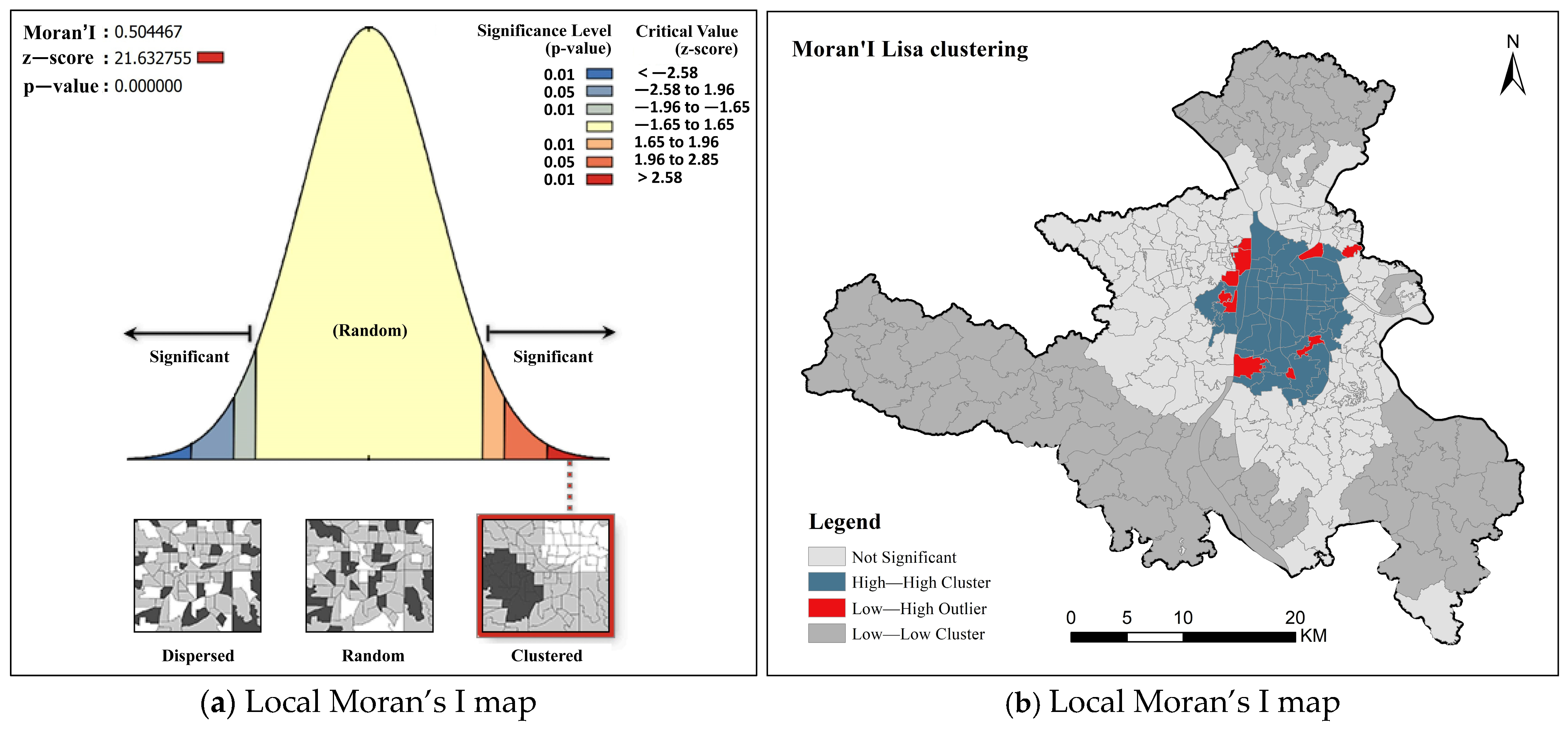
The global Moran’s I index (0.5045, p < 0.001) confirms a significant positive spatial autocorrelation for Urban Vitality across Changsha’s five districts in 2025. LISA cluster analysis reveals a spatial gradient of “single-core polarization, peripheral cold spots, and localized fragmentation,” driven by the structural coupling of urban planning, industrial allocation, and transport topology (Figure 8).
Specifically, High-High (HH) clusters (n = 47, 17.09%) are densely concentrated within the Wuyi Square commercial core and along the Xiangjiang River banks. Mechanistically, this is driven by high-density, mixed-use zoning integrated with a highly centric rail transit topology. Wuyi Square operates as the primary interchange for Metro Lines 1 and 2 (a classic TOD model), maximizing network closeness centrality and minimizing spatial friction for consumer flows. Under favorable land-rent mechanisms and floor-area-ratio incentives, this hyper-accessibility has clustered high-factor-density industries, such as modern services and the “influencer night economy,” turning the transit network into an element-capturing apparatus that funnels regional capital into the core.
Conversely, Low-Low (LL) clusters (n = 78, 28.36%) blanket peripheral zones, including western Yuelu, southern Tianxin, and northern Kaifu districts. This vitality deficit stems from institutional zoning constraints compounded by transport network marginalization. Under the “Changsha-Zhuzhou-Xiangtan Green Heart” regulatory framework, these spaces face rigid limits on development intensity and industrial entry thresholds, blocking incremental commercial development. Concurrently, sparse secondary road networks and a lack of rail transit extensions isolate these areas into physical “transportation islands,” preventing their rich ecological endowments from converting into socioeconomic assets.
Notably, Low-High (LH) outliers (n = 10, 3.63%) along the core’s margins reveal a powerful spatial siphon effect. The underlying mechanism is the “pipeline effect” of radial transport corridors, which traverse these transitional zones without establishing local industrial anchoring platforms. In this asymmetrical structure, the polarized core relentlessly extracts premium commercial capital and consumers from adjacent patches, structurally hollowing out peripheral borderlands into fragmented vitality voids. To mitigate this circle-layer solidification, future urban governance must transition Changsha into a multi-dimensional networked spatial structure (Figure 8). Strategic interventions should focus on deploying decentralized transport loops to break the unicentric monopoly, extending industrial axes from hubs like the Malanshan Digital Video Quarter, and fostering secondary vitality sub-centers (e.g., Meixihu New Town) to intercept regional production factors.

3.3. Analysis of Factors Influencing Urban Vitality

3.3.1. Model Evaluation and Cross-Validation

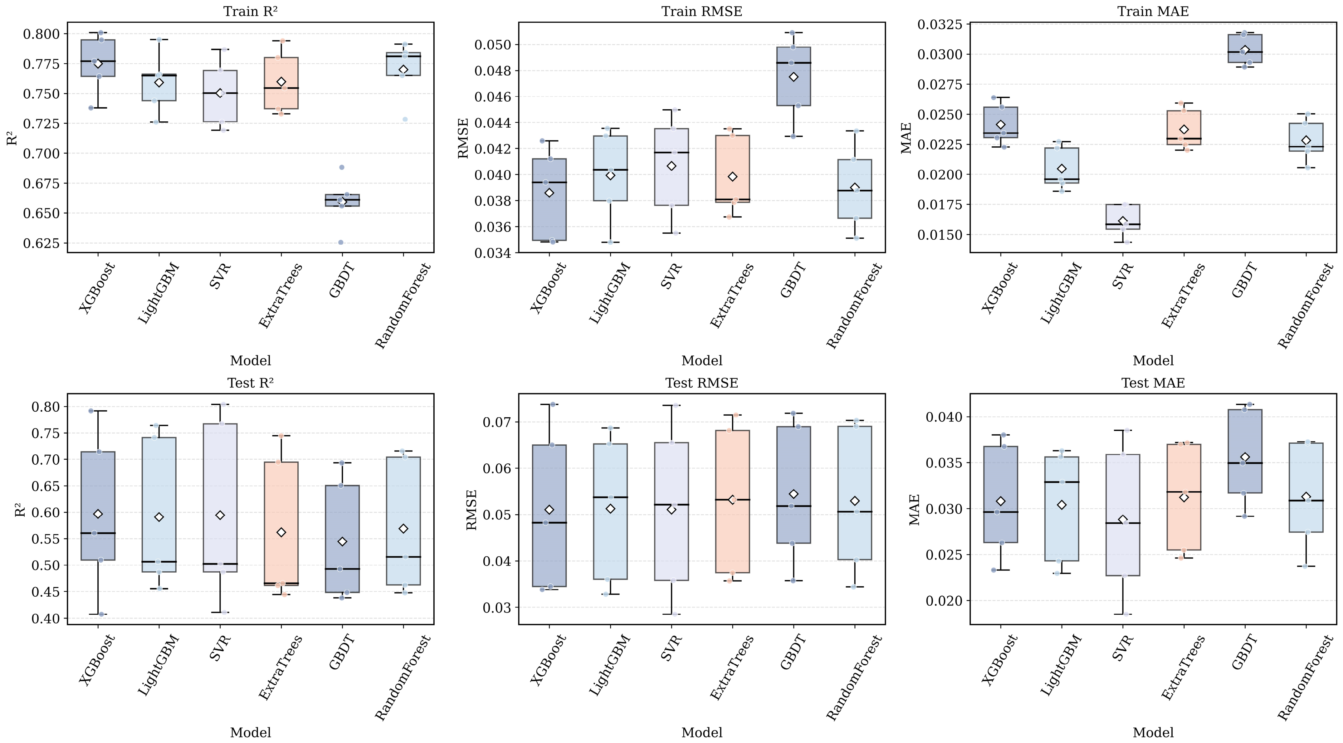
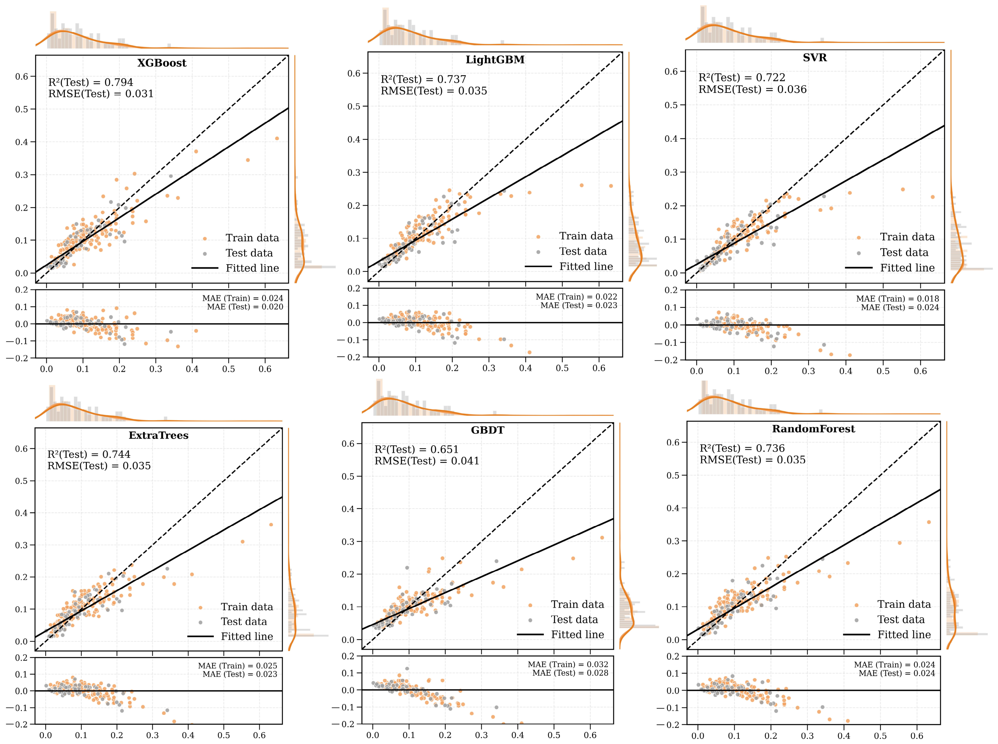
To comprehensively evaluate predictive performance, six machine learning models—namely Extra Trees, LightGBM, Random Forest, SVR, GBDT, and XGBoost—were systematically compared and evaluated (Figure 9).
On the standard test set, XGBoost achieved the superior global fit (R2 = 0.794, RMSE = 0.031, MAE = 0.020), accounting for approximately 79.4% of the variance in Urban Vitality with the lowest global prediction bias. However, these metrics are likely inflated by spatial autocorrelation. To strictly mitigate spatial adjacency artifacts, this study implemented a 5-fold spatial block cross-validation, partitioning the study area into five non-overlapping geographic blocks to ensure rigorous spatial separation between the training and testing sets during each iteration. The statistical summaries in Table 4, complemented by the boxplot distributions in Figure 10, confirm that this spatial blocking strategy successfully isolated adjacency effects, thereby providing a more realistic assessment of the models’ generalization limits.
Consequently, all models exhibited a performance decline on the test folds relative to the training folds, demonstrating that conventional global evaluations systematically overestimate predictive accuracy when spatial autocorrelation is present. Among the evaluated algorithms, XGBoost maintained the strongest generalization capability, yielding the highest mean R2 (0.5967) and the lowest RMSE (0.0511) on the test folds, which underscores its proficiency in capturing complex, non-linear spatial interactions. SVR and LightGBM remained highly competitive—with SVR capturing the absolute minimum Mean Absolute Error (MAE = 0.0288)—whereas GBDT performed the poorest across all metrics. Furthermore, the pronounced standard deviations of the test metrics across different spatial blocks highlight substantial spatial heterogeneity across the study area, indicating that the explanatory power of built environment determinants on Urban Vitality varies significantly across distinct geographic regions.
These generalization discrepancies and spatial block-level variances collectively reveal that while the global XGBoost model excels at mapping cross-sectional, systemic associations within the defined study boundary, its predictive generalizability to completely independent geographic contexts remains constrained by localized spatial dependencies. Consequently, it must be clearly stated that the reported non-linear thresholds and feature interpretations originate from a global model with limited spatial generalizability, and thus must be recognized strictly as context-specific environmental thresholds. These derived inflection points function as a localized diagnostic tool for the central districts of Changsha rather than universally transferable planning constants, and future cross-regional applications should re-calibrate the threshold bounds with caution to account for varying spatial autocorrelation behaviors.

3.3.2. Analysis of SHAP Global Interpretation Results

(1)
Feature importance analysis
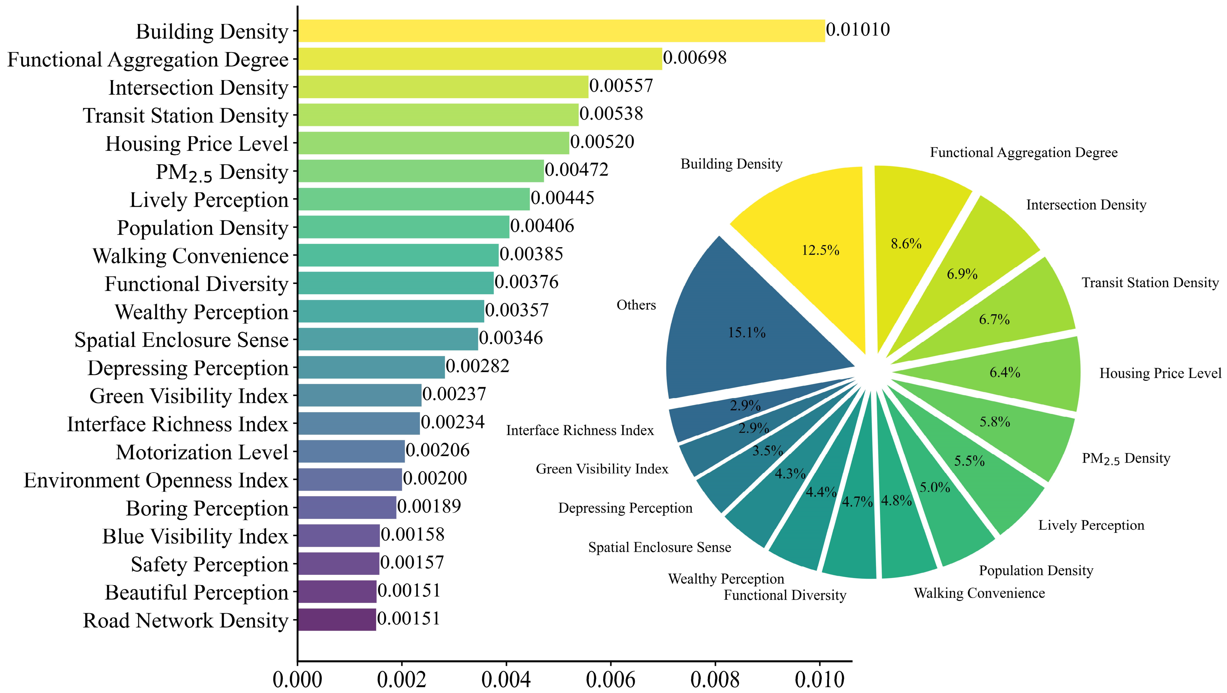
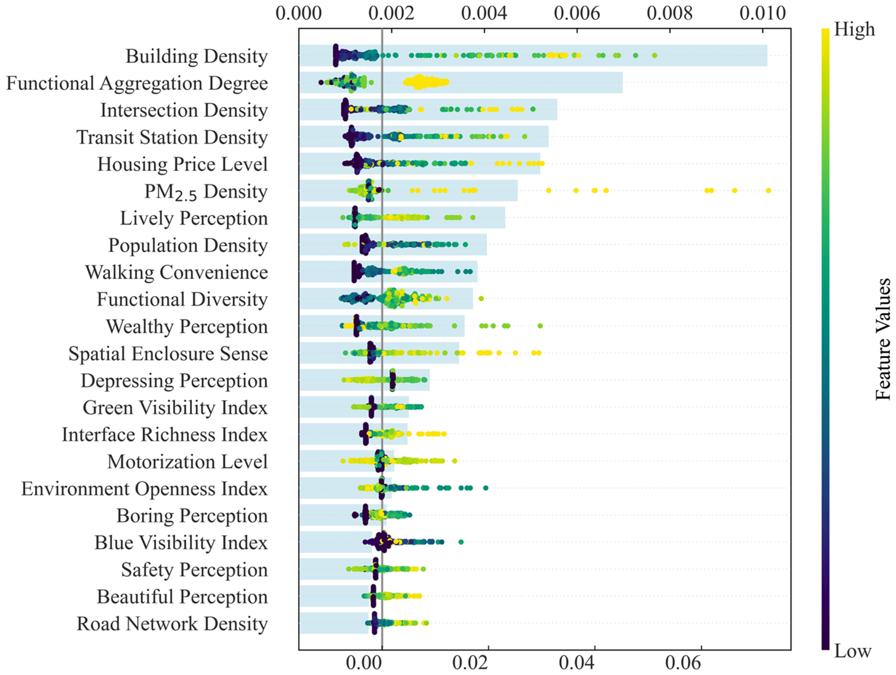
The global importance ranking based on the mean (|SHAP value|) reveals that Building Density, Functional Aggregation Degree, Intersection Density, Transit Station Density, Housing Price Level, and PM2.5 Density rank as the top six variables, the top 10 variables account for a cumulative contribution of approximately 66.95%. This indicates that comprehensive vitality is the outcome of multiple interacting factors (Table 5, Figure 11).
(2)
Analysis of the Honeycomb Plot.
The Honeycomb Plot of SHAP illustrates the directional effects of feature values across the variable spectrum (Figure 12).
For primary structural determinants, high feature values of both Building Density and Functional Aggregation are densely concentrated within the positive SHAP domain, validating that elevated physical density and Functional Aggregation Degree aggressively drive comprehensive Urban Vitality. Similarly, the rightward skew of high-value points for Intersection Density and Transit Station Density demonstrates that enhanced spatial connectivity and robust public transit provision serve as foundational infrastructure for vitality generation. Regarding market dynamics, the predominantly positive contributions of higher Housing Price Level imply that this metric captures a latent combination of premium locational value, superior public resource allocation, and intense market activity. Conversely, the behavior of environmental and perceptual indicators reveals nuanced spatial trade-offs. The distribution of PM2.5 Density presents a distinct pattern where high-value points intersect with positive SHAP regions in specific samples; rather than suggesting that pollution directly fosters growth, this variable operates as a symbiotic proxy signal for heavy traffic flows and high-density urban operations. Finally, high feature values for Lively Perception, Population Density, Walking Convenience, and Functional Diversity frequently cluster in the positive SHAP spectrum, indicating that Street View vitality, population aggregation, pedestrian convenience, and functional mixing can all improve comprehensive vitality under certain conditions.
(3)
Analysis of the Heatmap results
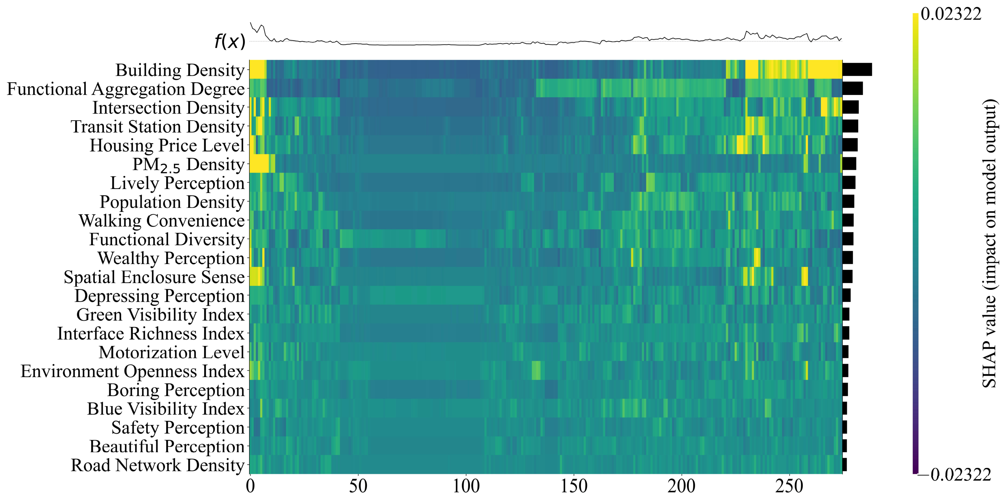
The SHAP Heatmap integrates both sample and variable dimensions into a single view (Figure 13), allowing for the observation of structural differences in contributions across various samples. The f(x) curve at the top of the figure illustrates the variation in the predicted values of the samples, the black bar chart on the right indicates the overall magnitude of variable contributions, and the Heatmap colors reflect the direction and magnitude of the SHAP contributions for each variable across individual samples. As shown in the Heatmap, Building Density, Functional Aggregation Degree, Intersection Density, Transit Station Density, Housing Price Level, and PM2.5 Density are located at the top, which is consistent with the SHAP importance ranking. These variables not only exhibit high average contributions but also demonstrate pronounced positive and negative shifts across samples, indicating that they are the primary sources of spatial heterogeneity in comprehensive vitality. In contrast, variables such as Road Network Density, Beautiful Perception, Safety Perception, and Blue Visibility Index display relatively weaker color bands overall, suggesting that they predominantly function as local modifiers.
Figure 13. Heatmap of Feature Distribution under Sample Clustering.
Systems 14 00842 g013

3.3.3. Analysis of Average Marginal Effects Based on PDP
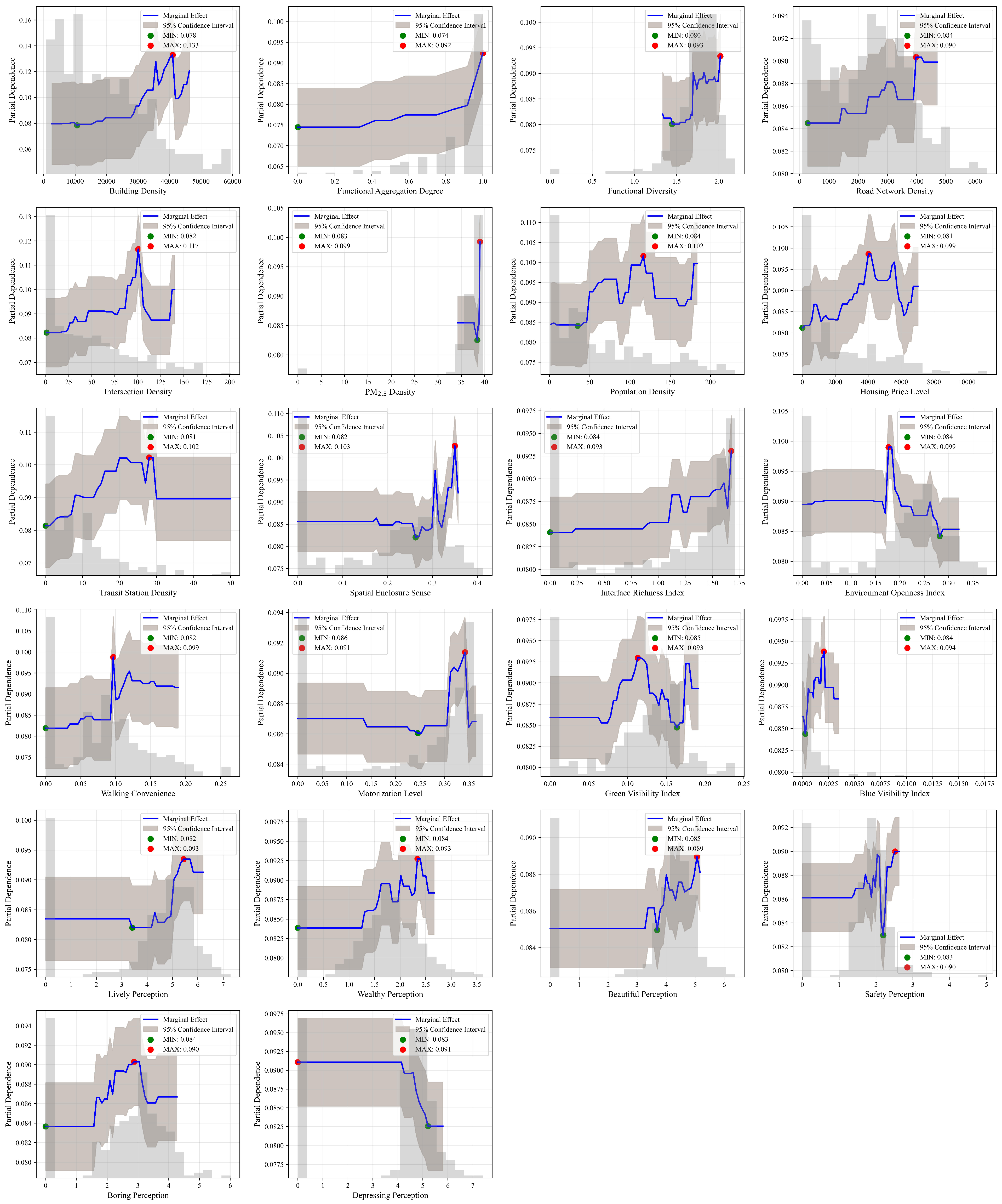
Partial Dependence Plots (PDP) reflect the average marginal effect of variations in an individual feature on the predicted comprehensive vitality, with the effects of all other features averaged out. Compared to SHAP dependence plots, PDP are better suited for identifying aggregated response characteristics, including overall increments, decrements, plateaus, inflection points, and diminishing marginal returns. (Figure 14).
Figure 14. PDP of variables.
Systems 14 00842 g014
The first category represents the continuous growth pattern, which includes Building Density, Functional Aggregation Degree, Functional Diversity, Interface Richness Index, Beautiful Perception, Lively Perception, and Safety Perception. The PDP curves reveal that the average marginal effect of Building Density overall exhibits a continuous upward trend. In low building density intervals, the predicted comprehensive vitality remains at a low level; when building density rises to approximately 25,000, the curve begins to elevate noticeably, entering a rapid growth stage within the 30,000 to 45,000 interval. Despite localized fluctuations at the high-value end, the marginal predicted value remains high overall, indicating that building density can significantly enhance comprehensive vitality once it reaches a certain scale. The PDP curve for Functional Aggregation Degree remains almost flat prior to 0.35, suggesting that low-to-moderate levels of functional clustering yield limited average improvements to comprehensive vitality. Subsequently, the curve climbs slowly and rises sharply as it approaches the high-value interval of 0.9–1.0. This variable exhibits a “high-clustering triggered” characteristic, meaning that functional aggregation significantly enhances the model’s predicted comprehensive vitality only when it reaches a relatively advanced degree. The PDP curve for Functional Diversity is primarily distributed within the 1.4–2.1 range; the curve fluctuates slightly in the low-to-medium value segments, initiates a gradual upward trend after approaching 1.7, and achieves a high marginal predicted value at the upper end. This indicates that functional diversity exerts a positive driving effect on comprehensive vitality, yet this effect does not increase linearly from low values but rather manifests progressively after crossing a certain functional compounding threshold. For the Interface Richness Index, the PDP curve is relatively flat before 1.0, commences its ascent after approximately 1.2, and exhibits a higher marginal predicted value above 1.6. This suggests that upgrading street interface richness helps amplify visual stimulation, activity accommodation, and commercial display capabilities, serving as a vital complementary variable for comprehensive vitality. The PDP curve for Beautiful Perception is relatively flat in the low-value segment, rises progressively after approximately 3.5, and reaches a high predicted value above 5.0. This demonstrates that streetscape aesthetics can positively supplement comprehensive vitality by reinforcing spatial attractiveness, the willingness to stay, and the sense of environmental quality. The PDP curve for Lively Perception remains basically flat from low values up to around 4.5, then climbs noticeably after 5.0, reaching a high predicted value around 5.5–6.0. This indicates that stronger perceived streetscape liveliness more readily enhances predicted comprehensive vitality; however, this promotion predominantly occurs in the higher perception intervals, characterizing it as a high-value enhancement variable. Lastly, the PDP curve for Safety Perception displays a fluctuating upward trend overall, experiencing an elevation around 2.0 followed by localized dips and rebounds. This indicates that perceived safety serves as a foundational baseline condition for the generation of comprehensive vitality—where an inadequate sense of safety restricts activity occurrence—while its marginal promotion following safety improvements remains moderated by functional and demographic contexts.
The second category represents the threshold leap pattern, which includes Transit Station Density, Walking Convenience, Spatial Enclosure Sense, PM2.5 Density, and Motorization Level. In this category, the PDP curve for Transit Station Density gradually climbs from a low baseline in the low-value segment, reaching a high level within the 10–20 interval, which indicates that transit station density can significantly enhance comprehensive vitality once it satisfies a baseline threshold. Past this high station density range, the curve plateaus or declines, hinting at a diminishing marginal return for public transit supply, and implying that the critical factor is not merely a quantitative increase but whether the station locations match functional clusters and human activity spaces. The PDP curve for Walking Convenience experiences a sharp, prominent leap around 0.10, reaching a localized peak before flattening out or minorly receding. This demonstrates that the promotion of comprehensive vitality is most pronounced when pedestrian convenience transitions from insufficient to moderate levels; however, further improvements do not necessarily yield continuous vitality enhancements, as its operational efficacy requires the synergistic coordination of functional diversity, intersection density, and street interfaces. For Spatial Enclosure Sense, the PDP curve is relatively flat before 0.25, elevates markedly as it approaches 0.3, and reaches a high plateau near 0.35. This suggests that an appropriate degree of enclosure can enhance street interface continuity, spatial containment, and the sense of place, thereby fostering comprehensive vitality. The PDP curve for PM2.5 Density is highly concentrated within the high-value interval of 38–40, while the low-value interval features sparse sampling and limited curve variation. As PM2.5 Density approaches the high-value end, the average predicted value undergoes a distinct leap. This result should not be interpreted as pollution directly driving vitality; rather, a more reasonable explanation is that PM2.5 Density serves as a proxy in the model, capturing the confounding, concomitant information of intense traffic, high built density, and dense human activities. Similarly, the PDP curve for Motorization Level is relatively flat in the low-value range, declines slightly near the median, and then climbs noticeably with distinct fluctuations in the 0.30–0.35 interval. This indicates that the motorization level possesses strong context-dependency; while moderate motorization may reflect traffic accessibility and road organizational capacity, its positive effect becomes unstable when it is excessive or mismatched with urban spatial forms.
The third category represents the inverted U-shaped or high-value recession pattern, which includes Population Density, Housing Price Level, Intersection Density, Environment Openness Index, Green Visibility Index, Boring Perception, Depressing Perception, and Wealthy Perception. Within this category, the PDP curve is lower in the low-value interval, then progressively elevates as Population Density increases, reaching a localized peak around 100–130. Thereafter, the curve exhibits declines and fluctuations, indicating that while population aggregation significantly fosters comprehensive vitality, excessive population density does not inevitably sustain vitality growth, and its eventual efficacy requires the mutual support of transport, functionality, and spatial quality. The PDP curve for Housing Price Level displays a fluctuating upward trend overall. The predicted values are lower in low housing price intervals, gradually climb as housing prices rise, and form a localized peak around 4000–5000. The high-value end continues to experience fluctuations, demonstrating that the housing price level functions more as a proxy variable for locational value, resource aggregation, and market prosperity rather than acting as a purely direct causal driver. The PDP curve for Intersection Density manifests a distinct non-linear ascent. It presents low predicted values in low intersection density intervals, progressively climbs with density increments, and reaches a prominent peak around 80–120. The subsequent recession and re-fluctuation at the high-value end suggest that intersection density is not simply a case of “the higher, the better”; rather, it optimizes spatial accessibility and route choice flexibility within a moderate-to-high connectivity interval. The PDP curve for the Environment Openness Index presents a structure characterized by an initial localized rise followed by a distinct decline. It reaches a brief peak near 0.20 but progressively trends downward after 0.23, entering a low-value plateau around 0.28. This suggests that excessive spatial openness dampens comprehensive vitality, which potentially corresponds to urban design disservices such as excessive building setbacks, weakened spatial boundaries, inadequate pedestrian containment, and oversized road scales. The PDP curve for the Green Visibility Index displays a multi-peak fluctuating structure, where the marginal predicted value rises noticeably within the 0.08–0.14 interval but recedes and fluctuates again in higher ranges. This reveals that green visibility does not monotonically promote comprehensive vitality; while an appropriate amount of greenery enhances environmental quality and staying comfort, excessive green volumes can obstruct street interfaces or dilute the visibility of commercial functions. Regarding negative streetscape perceptions, the PDP curve for Boring Perception rises within the 1.5–3.0 interval before leveling off or minorly receding. This outcome implies that the impact of a boring perception is non-linear; low-to-moderate levels of boredom do not significantly suppress vitality, though excessive boredom typically signifies a lack of spatial attractiveness. Conversely, Depressing Perception exhibits a highly rigid “high-value inhibition” characteristic. The curve maintains a high plateau prior to 4.5, but once it exceeds 4.8, it undergoes a precipitous, cliff-like drop, identifying it as one of the most critical negative streetscape perception variables requiring targeted intervention. Echoing these dynamics, the PDP curve for Wealthy Perception rises prominently after 1.2, reaches a relatively high plateau around 2.0–2.7, and subsequently exhibits a minor recession. This indicates that a higher perceived wealth status often aligns with superior streetscape quality, prime locational environments, and robust consumer activity foundations, which collectively bolster comprehensive vitality; however, an excessively high wealth perception may correspond to diminished spatial publicness or localized privatization and enclosure, causing its marginal effect to undergo a downward callback.
The fourth category represents the weak effect or sample-constrained pattern, which includes Road Network Density and Blue Visibility Index. Variables in this category exhibit lower independent marginal efficacy in model predictions, with narrow response amplitudes, playing auxiliary or indirect corrective roles within the vitality system. The PDP curve for Road Network Density displays a minor overall variation amplitude, exhibiting only a slow upward trend from low-to-medium intervals and a slight plateau at the high-value end. This indicates that while road network density carries a certain positive marginal effect on comprehensive vitality, its independent contribution is weak. The influence of road network density may instead be indirectly channeled through more direct accessibility metrics such as intersection density, walking convenience, and transit station density. For the Blue Visibility Index, the PDP curve is heavily clustered within an extremely low-value interval, representing a narrow overall sample distribution. The curve undergoes a localized, minor elevation as it transitions from near-zero to slightly higher values, but subsequently lacks sufficient sample support across the medium-to-high ranges. Consequently, this variable is more appropriately interpreted as a minor, secondary corrective factor for environmental quality rather than a core driving force of comprehensive vitality.

3.3.4. Analysis of Univariate Dependence Plots and Threshold Effects
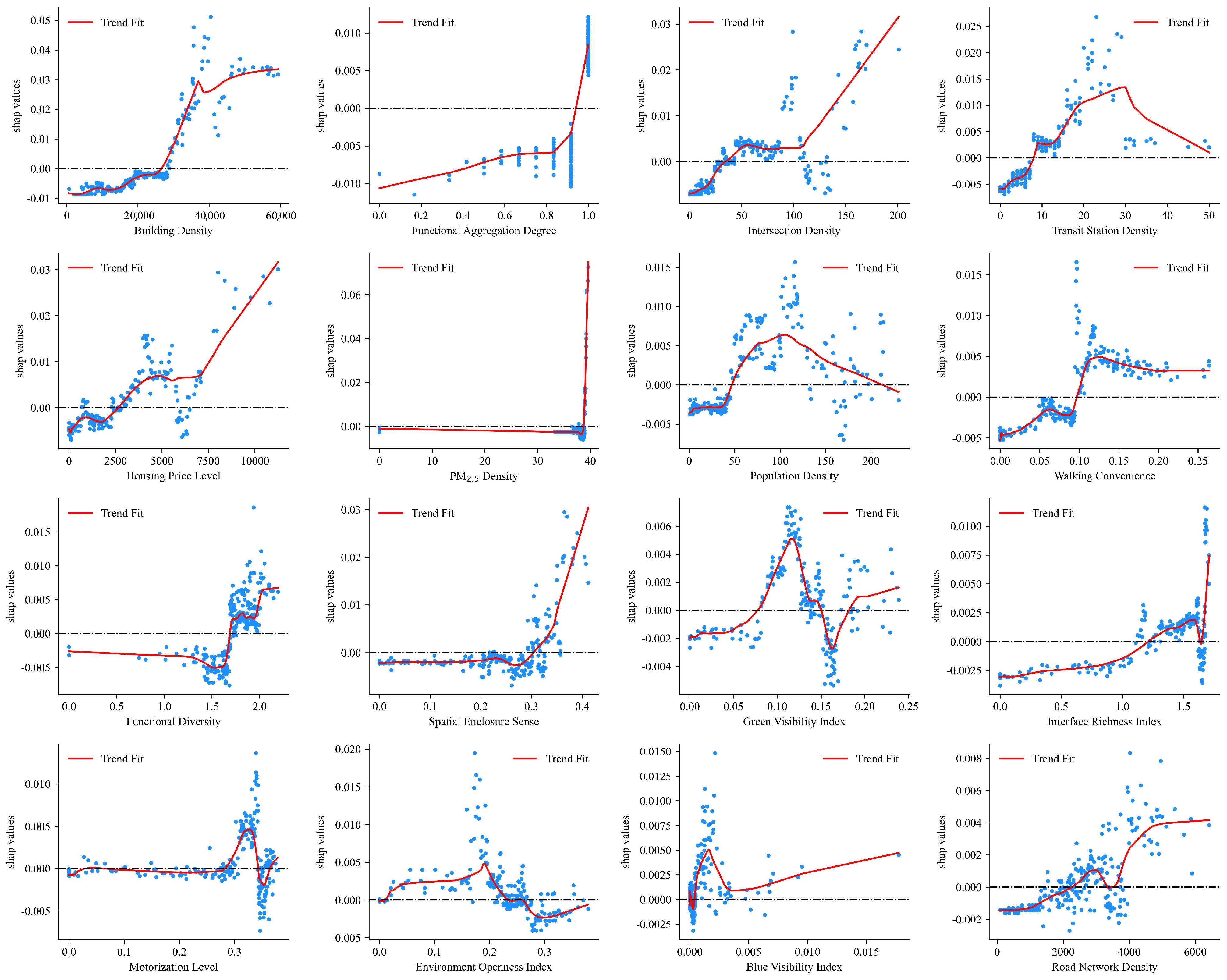
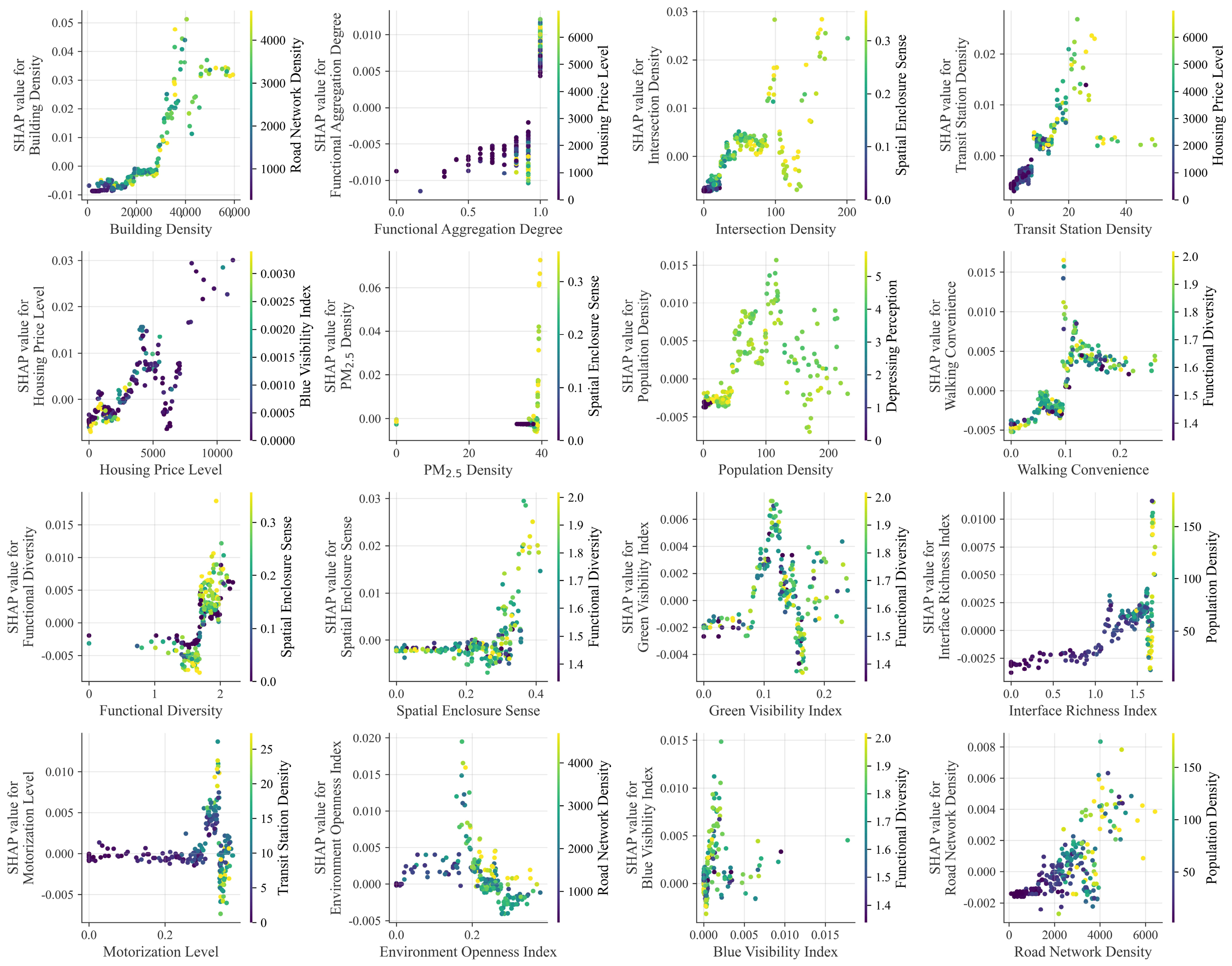
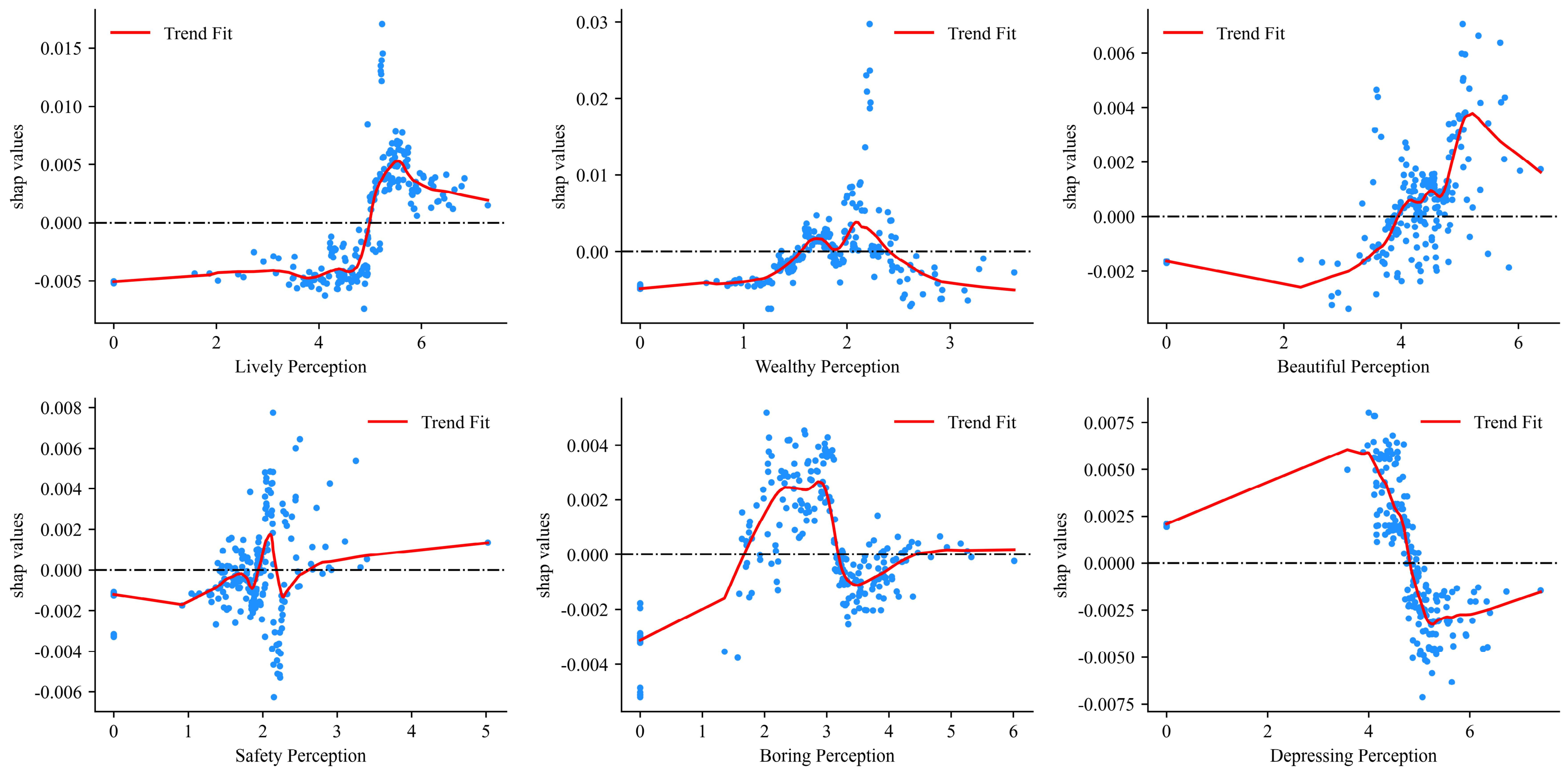
Following the identification of average marginal effects using PDP, SHAP dependence plots equipped with LOWESS fitting curves and threshold markers can further reveal the local contributions of variables within different value ranges. Unlike PDP, SHAP dependence plots illustrate the marginal contribution of a specific value to the model output within the context of the given sample. Therefore, they are better suited for explaining thresholds, points where contributions turn positive, plateau regions, and the dispersion caused by interaction backgrounds (Figure 15 and Figure 16). The determination of variable thresholds is based on the non-linear trend fitting results within the SHAP dependence plots. Specifically, the values of each predictor variable and their corresponding SHAP values are extracted first. The relationship between the variable values and the SHAP value is then modeled using the LOWESS (locally weighted scatterplot smoothing) method for local weighted smoothing fitting, thereby delineating the marginal impact trend of each variable on the model’s predictive outcomes. Subsequently, using a SHAP value of 0 as the reference baseline, interpolation and numerical solver methods are applied to identify the intersection points between the fitted curve and the horizontal line y = 0. The independent variable value corresponding to this intersection is defined as the potential threshold, which signifies the point around which the direction of the variable’s contribution to the predicted risk potentially shifts from negative to positive or vice versa. To ensure the rationality of the thresholds, only the intersection points falling within the actual range of variable observations are retained and are denoted with a red dashed line in the figures.
Figure 15. Objective environment univariate SHAP dependence plots.
Systems 14 00842 g015
Figure 16. Subjective perception univariate SHAP dependence plots.
Systems 14 00842 g016
Firstly, Typical threshold triggers positive effects. For Building Density, a threshold around 26,610 is identified; within the 30,000–40,000 range, SHAP values increase sharply, suggesting that this interval is particularly sensitive for vitality enhancement. Functional Aggregation Degree exhibits a threshold near 0.9, below this value, contributions are mostly non-positive, whereas approaching the threshold they become clearly positive, with stronger positive effects in the high-value region nearing 1.0. Intersection Density shows a threshold of approximately 34.6, beyond which SHAP values turn positive and continue to rise in the medium-to-high range; compared with road network density, it has relatively stronger explanatory power, and the dispersion in the high-value range implies that the relationship is not purely monotonic-moderately high connectivity, when combined with functional and interface support, appears to be most effective. Transit Station Density has a threshold around 8.0, the positive effect is rapidly released, but the curve flattens and even shows a slight pullback at very high densities, possibly due to service overlap or limited spatial carrying capacity. Finally, Lively Perception shows a threshold near 5.0, after which the SHAP value quickly turns positive and rises significantly; the slight pullback or spread at the upper end indicates that street-view vitality perception must be coordinated with physical functions, traffic, and population to maintain a stable positive contribution.
Secondly, Optimal interval suitability and diminishing marginal effects. Population Density exhibits two thresholds at approximately 47 and 213. Below the lower threshold, SHAP values are mostly negative or near zero, indicating insufficient aggregation and limited spatial utilization. Within the middle range (47–213), contributions remain positive, but beyond the upper threshold, the curve shows fluctuation and a partial pullback, suggesting diminishing returns. Functional Diversity has a threshold around 1.7, with the point cloud becoming more dispersed in the high-value zone (roughly 1.8–2.0). This implies that excessive functional mixing may lead to organizational conflicts or interface disorder, and its positive effect depends on coordination with spatial enclosure, walking convenience, and population density. Wealthy Perception presents thresholds at about 1.6 and 2.4; contributions gradually strengthen after surpassing 1.6, but the curve fluctuates and declines slightly beyond 2.4, indicating that while environmental quality enhances vitality, overly high levels may shift towards enclosure or reduced publicness. The Interface Richness Index shows multiple thresholds near 1.2, 1.6, and 1.7. Below 1.2, SHAP values tend to be negative, as a monotonous interface lacks attractiveness and activity capacity. Between 1.2 and 1.7, the values increase progressively, with a notable positive jump around 1.6–1.7, where enhanced richness improves street perceptibility and vitality. The Green Visibility Index has thresholds at roughly 0.08, 0.15, and 0.18; the curve begins to rise at 0.08, pulls back near 0.15, and fluctuates again near 0.18, marking it as a typical optimal-range variable. Spatial Enclosure Sense has a threshold of about 0.3, above which contributions increase rapidly and become strongly positive, as moderate enclosure reinforces boundary definition, continuity, and psychological safety, facilitating walking, staying, socializing, and consumption. Walking Convenience shows a threshold near 0.1; approaching this value, contributions turn positive and reach a local peak, but then pull back and fluctuate at higher levels, suggesting that mere convenience improvement without functional support is insufficient—it acts as a conditional facilitator. Finally, the Motorization Level presents multiple thresholds at 0.03, 0.07, 0.28, 0.34, and 0.36, with pronounced rises and fluctuations within the 0.28–0.36 range, and interwoven positive and negative contributions at high values, likely reflecting complex changes in motorized accessibility, road capacity, and regional traffic organization.
Thirdly, High-value suppression and significant inhibition effects. For the Environment Openness Index, multiple thresholds are observed at approximately 0.01, 0.23, 0.25, and 0.26. While moderate openness appears beneficial, the curve begins to decline when approaching 0.23, and the negative contribution becomes more pronounced beyond 0.25–0.26, suggesting that excessive openness may weaken the continuity of the street interface, the sense of spatial enclosure, and the capacity for staying, thereby reducing comprehensive vitality. For Depressing Perception, a threshold is found around 4.8; beyond this value, contributions decrease markedly and turn negative, indicating that this perception directly undermines individuals’ psychological comfort and willingness to stay, making it a primary inhibiting factor among negative street-view perceptions. For Boring Perception, multiple thresholds are identified at approximately 1.7, 3.2, and 4.4. The curve begins to pull back when approaching 3.2, and a distinct negative trend emerges approaching 4.4, implying that when boring perception reaches higher levels, issues such as monotonous spatial interfaces, insufficient activity stimuli, and weak place attractiveness begin to significantly diminish comprehensive vitality.
Fourthly, Environmental co-occurrence signals and auxiliary support effects. For Housing Price Level, a threshold is observed at approximately 2660. Below this value, SHAP values tend to be negative, suggesting insufficient public services, commercial resources, and transit convenience. Above the threshold, contributions turn positive and continue to rise, as higher housing prices often co-occur with better urban resources and higher activity intensity. However, the high-value range exhibits considerable dispersion, indicating that some high-price areas may not yield the highest vitality contribution, possibly due to single-functionality or spatial enclosure constraints. For PM2.5 Density, a threshold is found at roughly 38.7. In the low-to-medium range, SHAP values are near zero or slightly negative, implying that it is not a consistent vitality driver. At the high-value end, however, a notable upward jump occurs, which may reflect that high PM2.5 areas often coincide with heavy traffic, high activity density, and strong development intensit—rather than indicating a direct causal effect. For Road Network Density, multiple thresholds are identified at approximately 2266, 3342, and 3461. After crossing the first threshold, contributions turn positive and become relatively stable, yet the average SHAP value remains modest, and its explanatory power is partially absorbed by more specific connectivity variables (e.g., intersection density).
For Safety Perception, thresholds are observed at approximately 1.9, 2.2, and 2.6. Contributions gradually strengthen after exceeding 1.94, and a distinct positive contribution emerges in the 2.2–2.6 range, suggesting that enhanced safety perception is associated with improved willingness to use the spatial environment, making people more inclined to stay, socialize, and engage in daily activities in the streets. For Beautiful Perception, a threshold is found at roughly 4.9, beyond which it forms a stable positive contribution, implying that improving the aesthetic quality of street views may promote comprehensive vitality by enhancing visual quality, spatial comfort, and environmental attractiveness. Nevertheless, its overall explanatory strength ranks relatively low, indicating that beautiful perception can serve an “added-value” role, but the prerequisite is that the space already possesses a certain foundation of building density, functional capacity, and human activity. For the Blue Visibility Index, samples are highly concentrated in the extremely low range, making it difficult to identify a clear and stable threshold. With a slight increase in the index, SHAP values may exhibit a minor positive contribution, suggesting that blue space visibility might exert a certain auxiliary effect on comprehensive vitality by improving visual experiences, environmental comfort, or spatial recognizability.

3.3.5. Analysis of Bivariate Interaction Dependence Plots

Firstly, Building intensity and road network support mechanism. When Building Density is below 26,000, SHAP values are ≤0, and even a high Road Network Density is difficult to reverse this trend. After exceeding 30,000, SHAP values rise rapidly. Samples with high Road Network Density are concentrated in the high positive value region, indicating that Road Network Density has a distinct amplifying effect on the positive contribution of Building Density, forming a synergy of “high-intensity development coupled with high-connectivity network.” However, if Building Density is high but Road Network Density is insufficient, the positive contribution is still weakened. Road Network Density itself also exhibits thresholds; when it is below 2266, SHAP values are negative, after which they gradually turn positive, becoming more stable above 3000. Population Density exerts an amplifying effect on this: samples with high Population Density are more likely to form positive contributions within the high Road Network Density range. That is, the road network provides connectivity while population density provides travel demand; only when supply and demand are matched can they be translated into vitality.
Secondly, Functional aggregation and location value mechanism. Functional Aggregation Degree is primarily concentrated in the 0.8–1.0 range. In the low-aggregation stage, SHAP values are mostly negative, and the impact of Housing Price Level is limited. As it approaches 0.9, the SHAP value distinctly turns positive, and samples with a high Housing Price Level appear more frequently in the positive range. When Transit Station Density is below 8.0, SHAP values tend to be negative, which cannot be compensated for even by a high Housing Price Level. After exceeding 8.0, SHAP values turn positive and continue to rise in the 10–25 range, where samples with a high Housing Price Level are more likely to be located in the high positive contribution zone. Transit stations provide accessibility, while housing prices reflect locational demand; the combination of the two facilitates the formation of stable pedestrian flows and diverse activities, although diminishing marginal returns appear in ranges with extremely high station density. As Housing Price Level increases, the moderating intensity of the Blue Visibility Index is not as pronounced as that of density or functional variables. However, in some samples with high Housing Price Levels, a higher Blue Visibility Index can co-occur with high locational value, providing a certain supplementary enhancement to environmental quality.
Thirdly, Transportation nodes and activity Support Mechanisms. When Intersection Density is below 34.6, SHAP values are ≤0, which is difficult to reverse even with a high Spatial Enclosure Sense. After exceeding this threshold, contributions gradually turn positive, forming a stable positive contribution in the 50–100 range. Furthermore, samples with a higher Spatial Enclosure Sense are more likely to achieve higher SHAP value, indicating that the promoting effect of intersection density requires a moderate sense of enclosure to enhance the continuity, stability, and sense of place of the street interface. When Lively Perception approaches 5.0, SHAP values jump significantly, and samples with high Transit Station Density are more likely to form high contributions in the high Lively Perception region; this means that vitality perception and traffic channeling complement each other. When Walking Convenience is below 0.1, SHAP values are negative; they rise rapidly as the value approaches 0.10, where samples with higher Functional Diversity are more likely to generate positive contributions. This implies that Walking Convenience must be combined with sufficiently diverse functional destinations to truly translate into Urban Vitality.
When Functional Diversity is below 1.7, SHAP values are ≤0, gradually turning positive after exceeding this threshold; samples with a strong or moderate Spatial Enclosure Sense are more likely to gain positive contributions. Meanwhile, SHAP values rise rapidly as Spatial Enclosure Sense approaches and exceeds 0.3, and in the high-enclosure range, samples with higher Functional Diversity are more likely to form strong positive contributions. This interaction is a highly typical “spatial morphology-functional mix” synergistic mechanism within this model. When the Interface Richness Index is below 1.2, SHAP values are ≤0; they gradually rise beyond this point, reaching a higher contribution around 1.6. Samples with high Population Density are more likely to form high positive values in the high Interface Richness Index range, indicating that a rich interface requires the support of sufficient usage demand from the population. Motorization Level exhibits significant fluctuations in the 0.3–0.4 range, and samples with high Transit Station Density demonstrate stronger positive contributions in some medium-to-high motorization ranges. This suggests that motorized traffic and public transit may jointly constitute comprehensive accessibility; however, excessive motorization may weaken the pedestrian environment, thus requiring the support of transit supply and spatial functional conditions.
Fourthly, Street View quality and human demand mechanism. When PM2.5 Density is concentrated in the 38–40 range, there are very few samples in the low-value interval. Positive samples with high PM2.5 often appear in spatial contexts with a certain sense of enclosure and high activity intensity, indicating that this variable may capture a co-occurring signal of high-density built environments, traffic flow, human activity, and pollution exposure. When Population Density is below 47, SHAP value ≤0, turning positive as density increases. However, in areas with a strong Depressing Perception, even with high population density, SHAP values may pull back or exhibit strong dispersion. Depressing Perception transitions around 4.5–5.0; as it continues to rise, SHAP values rapidly decline and turn negative. When Depressing Perception is high, the overall contribution drops significantly, indicating that population aggregation cannot fully offset the impact of negative Street View perception. After Wealthy Perception reaches the 1.6–2.4 range, SHAP values rise significantly, and samples with high Population Density are more likely to generate high SHAP values in the high Wealthy Perception interval. This suggests that high-quality or high-end Street View environments are more easily translated into spatial vitality only when there is sufficient human activity demand. Beautiful Perception gradually turns positive after exceeding 3.9, and samples with high Population Density are more likely to form strong positive contributions in the high Beautiful Perception range, representing a synergy of “environmental attraction coupled with human demand.”
When the Green Visibility Index is in the low-to-moderate range, SHAP values gradually rise, indicating that an appropriate amount of visible greenery can improve street comfort, visual experiences, and environmental attractiveness. However, as it continues to rise, the curve pulls back and fluctuates with the fluctuation being related to Functional Diversity. That is, when functions are diverse, moderate greenery can serve as quality compensation, but excessive greenery may obstruct commercial interfaces. After the Environment Openness Index approaches 0.2–0.3, SHAP values drop significantly and turn negative; high Road Network Density does not stably offset this negative impact, corresponding to a situation where “excessive openness coupled with transit-oriented road networks” weakens vitality. Boring Perception and Depressing Perception exhibit a negative superimposition. Low-to-medium levels of Boring Perception merely reflect weak stimulation, but when both variables increase, SHAP values drop significantly, indicating a negative synergistic effect between boring and depressing perceptions. Values for the Blue Visibility Index are concentrated near 0, and its overall effect is weaker than that of density, functional, and traffic variables. Its local positive effect is more likely to manifest when Functional Diversity is high, acting as an environmental quality supplement in functionally rich areas. SHAP values for Safety Perception gradually rise in the 1.9–2.6 range, and samples with a high Functional Aggregation Degree are more likely to form a positive contribution after Safety Perception improves. This demonstrates that a sense of safety and functional opportunities must coexist: the sense of safety provides the behavioral foundation, while functional aggregation provides the purpose for activity—neither can be omitted (Figure 17 and Figure 18).
Furthermore, the scatter patterns and color distributions clearly support how these spatial synergies change across different times. When Building Density crosses 30,000, its SHAP value shoots up into a high positive range between 0.03 and 0.05. These high-value points are mostly green and yellow, representing high Road Network Density. This combination reflects the weekday “efficiency mechanism”, showing that high-density employment zones require strong road network support to handle peak commuting traffic. Unlike weekdays when people focus strictly on fast travel and ignore their surroundings, the weekend “experience mechanism” shows a completely different pattern in image. In the Spatial Enclosure Sense plot, while basic or low-enclosure areas contribute almost zero to vitality, the SHAP values jump sharply once reaching the comfortable interval of 0.30–0.35. These high-vitality points are predominantly yellow-green, indicating high Functional Diversity (1.8–2.0). This clear contrast proves that while weekdays prioritize traffic efficiency, weekends rely heavily on the combination of a human-scaled street enclosure and diverse commercial functions to successfully encourage leisure seekers to slow down, explore and stay.

4. Discussions and Conclusions

Based on the XGBoost model and the SHAPexplainable machine learning method, this study systematically explored the distribution of Urban Vitality and its influencing factors in the five administrative districts of Changsha. The main discussions and conclusions are as follows:

4.1. Discussion

  • Our results confirm that Building Density and Functional Aggregation Degree exhibit critical low-value inhibition, whereas Functional Diversity, Spatial Enclosure Sense, and Walking Convenience demonstrate narrow optimal-range configurations past which diminishing marginal returns emerge. Moving beyond traditional analyses [9,21], our interaction models utilize empirical evidence to explicitly define the structural boundaries between conditional coupling and positive synergy within these spatial relationships. Furthermore, our interaction models move beyond traditional segregated analyses.
Firstly, the interface between physical urban mass, land-use intensity, and network configuration operates strictly as a mechanism of conditional coupling, where a primary baseline must be satisfied before secondary elements generate positive utility. The interaction between Building Density and Road Network Density proves that high density yields suboptimal utility if decoupled from road network support. Spatially, in structurally sparse zones like the newly developing, fragmented peri-urban fringes of western Yuelu District (such as the low-density industrial extensions around the Jianshan Lake or Pingtang sectors), expanding local road grids remains economically inert because the built volume is too low to anchor human activities; once this morphological baseline crosses the critical threshold ≈ 26,610.13, the interaction shifts into positive synergy, where network connectivity actively multiplies the returns of development intensity. Similarly, Functional Aggregation Degree exhibits a rigid conditional coupling boundary at its activation threshold ≈ 0.94, proving that highly scattered land layouts actively suppress vitality; substantial gains are unlocked only when resources surpass this milestone into a hyper-concentrated commercial-service cluster—a phenomenon epitomized by the dense, self-reinforcing service ecosystem of the Wuyi Square core. Concurrently, the coupling of Walking Convenience and Functional Diversity demonstrates another conditional coupling layer, wherein pedestrian walkability fails to independently amplify vitality unless structurally accommodated by functional diversity. This mirrors the wide, car-centric superblocks in newly built areas of Changsha (such as the oversized residential blocks in Yuelu or Meixihu New Town), where sidewalk networks are squandered as empty channels unless matched with a diverse land-use mix exceeding the threshold (1.69) necessary to establish at least 3–4 distinct destination categories (retail, dining, local amenities) to motivate multi-purpose pedestrian trips.
Secondly, the alignment of network topology and street morphology operates via a clear mechanism of positive synergy, defined as a mutual amplification process where elements continuously reinforce each other’s marginal returns. The interaction between Intersection Density and Spatial Enclosure Sense confirms that network connectivity requires an optimal enclosure ratio ≈ 0.30–0.35 to capture vitality. This represents the human-scaled 1:3 to 1:2 street height-to-width proportion found in Changsha’s traditional downtown commercial alleys (such as Huangxing South Road Pedestrian Street, Taiping Street, or the historical lanes peripheral to Pozi Street), which transforms rapid transit corridors into comfortable urban containers that optimize pedestrian thermal comfort, protect against wind-tunnel effects, and encourage public stability. Consequently, stock urban renewal must shift from single-element patching to the systemic upgrading of four structural pairs: “Building Density–Road Network support” “Functional Aggregation-location value” “Transportation node-activity accommodation” and “Street View quality-human demand.”
2.
Leveraging the “two-way regulation” of Subjective Perception to achieve precise interventions through micro-renewal. As shown in the fourth mechanism (Street View quality–human demand), positive perceptions—such as Beautiful Perception, Wealthy Perception, and the Interface Richness Index—rely on Population Density as a foundational demand to stably enhance vitality. Specifically, areas with higher Population Density exhibit stronger positive contributions within high-beauty, high-wealth, and high-interface-richness ranges. Spatially, this operational boundary represents a mechanism of demand-driven positive synergy, where aesthetic or quality enhancements do not independently generate vitality but serve as visual modifiers whose real-world utility requires a critical mass of human activity; without an adequate local population, such enhancements remain economically inert. Meanwhile, Lively Perception (threshold ≈ 4.99) and Transit Station Density demonstrate a complementary positive synergy, where perceptual vibrancy and traffic channeling jointly amplify vitality, illustrating a mutual reinforcement process where high-frequency transit nodes continuously pump pedestrian flows that organically feed into and sustain active street-level commercial interfaces.
Conversely, negative perceptions like Depressing Perception (threshold ≈ 4.82) and Boring Perception (thresholds ≈ 3.19 and 4.43) impose a mechanism of rigid negative inhibition at higher values, acting as an absolute psychological barrier that caps the area’s underlying development potential. The interaction between Depressing Perception and Population Density reveals that severe spatial oppression counteracts the benefits of population aggregation, causing SHAP values to decline or disperse. Spatially, this rigid inhibition isolates degraded, poorly maintained, or barrier-heavy streetscapes—such as the dark, uninviting pedestrian environments underneath the massive overhead concrete infrastructure of the Furong Mid-road elevated expressway or the long, continuous blank boundary walls fencing off older gated high-rise residential compounds; once this depressing threshold is breached, the spatial discomfort completely repels public stability regardless of the surrounding population concentration. Furthermore, a negative synergistic superimposition exists between Boring Perception and Depressing Perception, leading to a destructive compounding effect where visual monotony and environmental oppression interact simultaneously to accelerate the desertion of the public realm. Consequently, urban renewal must prioritize eliminating visual dullness and spatial oppression, balancing “landscape demonstrability” with “daily publicness.” Implementing low-cost interventions—such as diverse commercial spillover spaces, window displays, and soft interfaces—can leverage this perceptual multiplier effect to optimize existing urban functions and populations.
3.
Addressing Urban Vitality polarization and the siphon effect by identifying spatial vitality “collapse zones” and promoting “gradient transmission”. Spatial autocorrelation analysis indicates that Urban Vitality exhibits strong spatial aggregation (Global Moran’s I = 0.5045, p < 0.001). Local Indicators of Spatial Association (LISA) clustering reveals a gradient structure characterized by single-core polarization, peripheral cold spots, and local fractures. Specifically, High-High clusters (47, 17.09%) converge around the Wuyi Square core business district and the banks of the Xiangjiang River, where social, economic, and cultural vitalities are deeply coupled in a self-reinforcing loop of positive synergy fueled by multi-line TOD infrastructure and dense commercial aggregation. Conversely, Low-Low clusters (78, 28.36%) span peripheral zones—such as western Yuelu, southern Tianxin, and northern Kaifu districts—acting as spatial depressions in the comprehensive evaluation despite their ecological endowments. Spatially, this operational boundary marks a mechanism of rigid institutional and infrastructural inhibition; under the strict regulatory redlines of the “Changsha-Zhuzhou-Xiangtan Green Heart” ecological framework in southern Tianxin, land-use intensity is restricted, freezing these ecological zones into physical “vitality depressions” unable to convert green assets into daily public activity. Low-High outliers (10, 3.63%) peripheral to the core area signify a pronounced siphon effect, which operates through a negative spatial conflict of asymmetrical element extraction, where radial transit extensions act as pipelines that rapidly pull capital and consumer populations out of intermediate transitional neighborhoods and channel them into the polarized Wuyi Square core. SHAP heatmaps further substantiate the spatial differentiation in the marginal contributions of core variables (e.g., Building Density, Functional Aggregation Degree, and Intersection Density), showing positive contributions dominating the central urban area and negative contributions prevailing in peripheral zones. Consequently, urban planning must eschew undifferentiated regulation. For siphon zones, enhancing endogenous attractiveness via micro-renewal, shared infrastructure, and digital cultural tourism is critical to mitigating unidirectional element outflow. Conversely, for the stagnant Low-Low clusters, priority should be given to improving foundational elements, such as Building Density and Road Networks, to breach development thresholds and gradually establish a resilient network characterized by bidirectional element flows and vitality gradient transmission.
4.
Disentangling “confounding synchronous indicators” to decouple statistical co-occurrence from true causality. To avoid urban planning fallacies, it is crucial to rationally examine confounding synchronous indicators within the model by separating causal positive synergies from conditional environmental costs. Although PM2.5 Density and Housing Price Level rank among the top six variables in feature importance (contributing 5.84% and 6.44%, respectively), they represent accompanying manifestations rather than direct drivers of Urban Vitality. The positive contribution of high PM2.5 Density represents a mechanism of environmental co-occurrence rather than causality. Elevated pollution metrics do not foster urban growth; instead, they serve as a downstream physical signal of the hyper-dense built configurations and heavy traffic volumes native to active urban cores. This is further substantiated by the interaction between PM2.5 Density and Spatial Enclosure Sense, which shows that high-PM2.5 positive samples cluster exclusively within tightly enclosed, hyper-active downtown street canyons. Meanwhile, Housing Price Level (threshold ≈ 2658.99) acts as a locational value proxy that captures resource aggregation. Its interactions with Functional Aggregation Degree and Transit Station Density indicate a conditional coupling relationship, where the robust purchasing power inherent to premium real estate enclaves facilitates the release of vitality effects from functional mixes and transit hubs. However, our analysis uncovers a critical high-value constraint where housing prices trigger a negative pullback at extreme configurations (4000–5000). Spatially, this corresponds to upscale, single-use gated luxury communities in Changsha, where excessive perimeter enclosure, low land-use mix, and private security protocols reduce public accessibility and suppress street-level public life. Therefore, planning interventions should prioritize optimizing functional organization to mitigate the negative externalities of high-intensity aggregation, resolutely avoiding the fallacy of misinterpreting environmental costs as indicators of vitality enhancement. Concretely, this entails deploying urban ventilation corridors and expanding street-side greenery to alleviate high-PM2.5 environmental costs, alongside distributing basic public facilities equitably to decentralize the resource advantages of high-housing-price enclaves and catalyze peripheral vitality.
Limitations and Future Directions. Although the XGBoost-SHAP framework provides quantifiable thresholds for vitality diagnosis, several limitations persist. Firstly, SHAP attributions reflect statistical correlation rather than absolute causality. Secondly, multi-source datasets present potential spatiotemporal misalignment between static street-view imagery and dynamic population aggregation. Thirdly, visual perception metrics suffer from sampling bias, creating structural blind spots regarding indoor complexes and pedestrian back-alleys. Finally, the derived thresholds are sample-dependent, requiring cross-city recalibration for generalization. Future studies should integrate causal inference tools (e.g., DID and instrumental variables) and multi-scale temporal datasets to empirically validate the causal pathways of these critical spatial variables.

4.2. Conclusions

This study transcends traditional “linear driving” and “single-element superimposition” paradigms in urban vitality research. Instead, it introduces a comprehensive analytical framework integrating XGBoost-SHAP explainable machine learning with multi-source geospatial data. By scrutinizing objective environment alongside subjective perceptions, it conceptualizes and validates Urban Vitality as a multi-dimensional, nested, and highly non-linear complex system. The primary conclusions are articulated as follows:
  • Threshold constraints and synergistic coupling of built environments. Within the specific geographic boundaries of this study area, the generation of Urban Vitality is bounded by localized non-linear spatial thresholds and synergistic constraints. The positive externalities of physical environment attributes exhibit distinct “activation milestones” and “iminishing marginal returns” rather than infinite monotonic growth. Crucially, while the precise numerical intervals of these identified thresholds are highly specific to the spatial fabric of the study region and possess limited external generalizability to independent geographic contexts, they demonstrate a valuable methodological template. Consequently, stock-era urban renewal within similar metropolitan contexts must abandon extensive incremental expansion in favor of the precise, localized allocation of core resources, unlocking non-linear vitality leaps through the strategic coupling of development intensity, transport networks, and functional configurations.
  • Human-oriented perceptual regulation and conversion efficiency. Human-centric spatial perception serves as the critical nexus determining the conversion efficiency of Urban Vitality. Detaching physical environment enhancements from the visual and psychological demands of residents inevitably precipitates a spatial resource mismatch. The observed two-way regulatory effects of subjective perceptions demonstrate that mitigating spatial oppression and upgrading interface interaction quality are cost-effective pathways for spatial revitalization within existing functional and demographic frameworks.
  • Evidence-based and differentiated urban governance. Urban governance in the stock era requires an evidence-based, differentiated regulatory paradigm. To mitigate intensifying vitality polarization and spatial siphoning, planning policies must look beyond statistical co-occurrence to uncover authentic causal mechanisms. Future spatial planning should shift from a globally uniform approach to targeted micro-renewal guided by quantitative diagnostics, prioritizing the remediation of “vitality collapse zones” in peripheral and siphon areas.
In summary, this study advances the methodological frontier of non-linear evaluation and interaction mechanism analysis for Urban Vitality. Concurrently, it provides a scientific foundation and empirical reference for promoting human-centric micro-renewal, optimizing spatial resource allocation, and fostering high-quality urban living environments.

Author Contributions

Conceptualization, H.W. and L.Z.; methodology, H.W. and L.Z.; software, H.D.; validation, H.W., L.Z. and Q.C.; formal analysis, H.W.; investigation, H.W.; resources, L.Z.; data curation, H.W. and H.D.; writing—original draft preparation, H.W.; writing—review and editing, L.Z. and Q.C.; visualization, H.W. and H.D.; supervision, L.Z. and Q.C.; project administration, L.Z. and Q.C.; funding acquisition, L.Z. All authors have read and agreed to the published version of the manuscript.

Funding

This research was funded by The National Social Science Fund of China, grant number 19ZDA191.

Data Availability Statement

The datasets can be provided by the corresponding author upon reasonable request.

Acknowledgments

We would like to thank the editor and the anonymous referees for their time and feedback which substantially improved this work.

Conflicts of Interest

The authors declare no conflicts of interest.

References

  1. Mouratidis, K.; Delclòs-Alió, X. Urban Vitality versus Urban Livability: Does Vibrancy Matter for Neighborhood Satisfaction and Neighborhood Happiness? Cities 2026, 168, 106473. [Google Scholar] [CrossRef] [Scilit]
  2. Implementation Plan for New Urbanization During the 14th Five-Year Plan Period. Available online: https://www.ndrc.gov.cn/fggz/fzzlgh/gjjzxgh/202207/t20220728_1332050.html (accessed on 23 May 2026). (In Chinese)
  3. Jacobs, J. The Death and Life of Great American Cities; Random House: New York, NY, USA, 2015. [Google Scholar]
  4. Montgomery, J. Making a city: Urbanity, vitality and urban design. J. Urban Des. 1998, 3, 93–116. [Google Scholar] [CrossRef] [Scilit]
  5. Wang, Z.; Xu, W.; Liu, Y.; Liu, B.; Zhu, L. Urban Vitality Transfer: Analysis of 50 Factors Based on 24-h Weekday Activity in Nanjing. Front. Archit. Res. 2025, 14, 1249–1273. [Google Scholar] [CrossRef] [Scilit]
  6. Jiang, Y.; Han, Y.; Liu, M.; Ye, Y. Street vitality and built environment features: A data-informed approach from fourteen Chinese cities. Sustain. Cities Soc. 2022, 79, 103724. [Google Scholar] [CrossRef] [Scilit]
  7. Sheng, J.; He, Y.; Lu, T.; Wang, F.; Huang, Y.; Leng, B.; Zhang, X.; Chen, Y. Unveiling Urban Vitality and Its Interactions in Mountainous Cities: A Human Behaviour Perspective on Community-Level Dynamics. Cities 2025, 159, 105780. [Google Scholar] [CrossRef] [Scilit]
  8. Tartari, M.; Pedrini, S.; Sacco, P.L. Urban ‘Beautification’ and Its Discontents: The Erosion of Urban Commons in Milan. Eur. Plan. Stud. 2022, 30, 643–662. [Google Scholar] [CrossRef] [Scilit]
  9. Ewing, R.; Cervero, R. Travel and the Built Environment: A Meta-Analysis. J. Am. Plan. Assoc. 2010, 76, 265–294. [Google Scholar] [CrossRef] [Scilit]
  10. Zhan, D.; Wang, Y.; Wu, Q.; Zhang, W. Nonlinear Effects of the Urban Built Environment on Urban Vitality: A Case Study of Hangzhou, China. J. Geogr. Sci. 2025, 35, 1183–1203. [Google Scholar] [CrossRef] [Scilit]
  11. Chen, Y.; Yu, B.; Shu, B.; Yang, L.; Wang, R. Exploring the Spatiotemporal Patterns and Correlates of Urban Vitality: Temporal and Spatial Heterogeneity. Sustain. Cities Soc. 2023, 91, 104440. [Google Scholar] [CrossRef] [Scilit]
  12. Yang, D.; Wang, X.; Han, R. Nonlinear and Synergistic Effects of the Built Environment on Street Vitality: The Case of Shenyang. Urban Plan. Forum 2023, 5, 93–102. (In Chinese) [Google Scholar] [CrossRef]
  13. Shao, J.; Long, Y.; Liu, X.; Zheng, Y.; Song, Y.; Wang, J.; Liu, B.; Yang, J.; Chen, Y.; Zhang, F. Machine Learning-Based Study on Factors Influencing Street Vitality in Urban Fringe Commercial Districts: A Case of Wuhan. Front. Archit. Res. 2026, 15, 582–608. [Google Scholar] [CrossRef] [Scilit]
  14. Zhang, Y.; Wang, X.; Ye, Y.; Wang, L.; Zhang, Y.; Qin, W.; Chi, Y.; Liu, G.; Yao, S. Nonlinear Relationships and Interaction Effects of Urban Built Environment on Urban Vitality Based on Explainable Machine Learning. City Environ. Interact. 2025, 28, 100244. [Google Scholar] [CrossRef] [Scilit]
  15. Yuan, L.; Dan, Y.; Leng, Y.; Zhang, J. Influencing Factors of Urban Safety Perception Based on the Combination of Multi-SouSrce Data and Machine Learning: A Case Study of Nanchang City, China. Sci. Rep. 2025, 16, 3972. [Google Scholar] [CrossRef] [Scilit] [PubMed]
  16. Han, C.; Zhang, Z. Nonlinear Effects of Built Environment Perception and Objective Features on Street Vitality in Historic Districts. Front. Archit. Res. 2026, 15, 1075–1091. [Google Scholar] [CrossRef] [Scilit]
  17. Wu, Z.; Zheng, M.; Zhang, T. Impact Characteristics and Interaction Effects of Built Environment on Street Space Quality in Megacities: A Case Study of Xi’an, China. City Environ. Interact. 2025, 28, 100257. [Google Scholar] [CrossRef] [Scilit]
  18. Lee, S.; Cho, N. Nonlinear and Interaction Effects of Multi-Dimensional Street-Level Built Environment Features on Urban Vitality in Seoul. Cities 2025, 165, 106145. [Google Scholar] [CrossRef] [Scilit]
  19. Doan, Q.C.; Zhang, X. A Systematic Review of Urban Vitality Studies: Trends and Research Opportunities. Land Use Policy 2025, 158, 107745. [Google Scholar] [CrossRef] [Scilit]
  20. Guo, H.; Zhang, S.; Xie, X.; Liu, J.; Ho, H.C. Moderation effects of streetscape perceptions on the associations between accessibility, land use mix, and bike-sharing use: A cross-sectional study. JMIR Public Health Surveill. 2024, 10, e58761. [Google Scholar] [CrossRef] [Scilit] [PubMed]
  21. Liu, Y.; Liu, X.; Gao, S.; Gong, L.; Kang, C.; Zhi, Y.; Chi, G.; Shi, L. Social sensing: A new approach to understanding our socioeconomic environments. Ann. Assoc. Am. Geogr. 2015, 105, 512–530. [Google Scholar] [CrossRef] [Scilit]
  22. Liu, J.; Wang, B.; Xiao, L. Non-Linear Associations between Built Environment and Active Travel for Working and Shopping: An Extreme Gradient Boosting Approach. J. Transp. Geogr. 2021, 92, 103034. [Google Scholar] [CrossRef] [Scilit]
  23. Shi, Y.; Zheng, J.; Pei, X. Measurement Method and Influencing Mechanism of Urban Subdistrict Vitality in Shanghai Based on Multisource Data. Remote Sens. 2023, 15, 932. [Google Scholar] [CrossRef] [Scilit]
  24. Zhu, T.; Tu, W.; Yue, Y.; Zhong, C.; Zhao, T.; Li, Q.; Li, Q. Sensing Urban Vibrancy Using Geo-Tagged Data. Acta Geod. Cartogr. Sin. 2020, 49, 365–374. [Google Scholar] [CrossRef]
  25. Wang, X.; Zhang, Y.; Yu, D.; Qi, J.; Li, S. Investigating the Spatiotemporal Pattern of Urban Vibrancy and Its Determinants: Spatial Big Data Analyses in Beijing, China. Land Use Policy 2022, 119, 106162. [Google Scholar] [CrossRef] [Scilit]
  26. Huang, H.; Shi, H.; Li, X.; Wang, Y. Exploring the Recreational Micromobility in Relation to Historic Urban Areas and Social Media: Insights from Machine Learning Approaches. Landsc. Urban Plan. 2025, 263, 105447. [Google Scholar] [CrossRef] [Scilit]
  27. Gao, C.; Li, S.; Sun, M.; Zhao, X.; Liu, D. Exploring the Relationship between Urban Vibrancy and Built Environment Using Multi-Source Data: Case Study in Munich. Remote Sens. 2024, 16, 1107. [Google Scholar] [CrossRef] [Scilit]
  28. Xu, Y.; Mao, W.; Hu, S. Unveiling the Pulse of Urban Metro Stations: A TOD-Driven Approach to Measuring Vibrancy Using Geographically Weighted Random Forest. Int. J. Digit. Earth 2025, 18, 2524054. [Google Scholar] [CrossRef] [Scilit]
  29. Ling, Z.; Zheng, X.; Chen, Y.; Qian, Q.; Zheng, Z.; Meng, X.; Kuang, J.; Chen, J.; Yang, N.; Shi, X. The Nonlinear Relationship and Synergistic Effects between Built Environment and Urban Vitality at the Neighborhood Scale: A Case Study of Guangzhou’s Central Urban Area. Remote Sens. 2024, 16, 2826. [Google Scholar] [CrossRef] [Scilit]
  30. Xia, X.; Zhang, Y.; Zhang, Y.; Rao, T. The Spatial Pattern and Influence Mechanism of Urban Vitality: A Case Study of Changsha, China. Front. Environ. Sci. 2022, 10, 942577. [Google Scholar] [CrossRef] [Scilit]
  31. Lian, A.; Zhang, Y.; Cai, Y.; Wang, Z.; Sun, X.; Jiao, Y.; Dong, R. Exploring the Nonlinear Relationship and Interaction Effects between the Built Environment and Street Vitality Using Machine Learning Methods. Ecol. Front. 2026, 46, 932–946. [Google Scholar] [CrossRef] [Scilit]
  32. Huang, Y.; Du, J.; Chen, M.; Lin, Y.; Huang, S.; Cai, Y. Evaluating the Spatial-Temporal Impact of Urban Nature on Urban Vitality in Vancouver: A Social Media and GPS Data Approach. Land Use Policy 2026, 160, 107824. [Google Scholar] [CrossRef] [Scilit]
  33. Huang, Y.; Zheng, B. Social Media Users’ Visual and Emotional Preferences of Internet-Famous Sites in Urban Riverfront Public Spaces: A Case Study in Changsha, China. Land 2024, 13, 930. [Google Scholar] [CrossRef] [Scilit]
  34. Yang, C.; Zhang, Y. Public emotions and visual perception of the East Coast Park in Singapore: A deep learning method using social media data. Urban For. Urban Green. 2024, 94, 128285. [Google Scholar] [CrossRef] [Scilit]
  35. Bao, W.; Gong, A.; Zhang, T.; Zhao, Y.; Li, B.; Chen, S. Mapping Population Distribution with High Spatiotemporal Resolution in Beijing Using Baidu Heat Map Data. Remote Sens. 2023, 15, 458. [Google Scholar] [CrossRef] [Scilit]
  36. Yu, M.; Ji, Q.; Zheng, X.; Cui, W. Nonlinear Effects of the Built Environment on Urban Vitality in Jinan Based on Multi-Source Data and Explainable AI. Sci. Rep. 2026, 16, 4923. [Google Scholar] [CrossRef] [Scilit] [PubMed]
  37. Montalto, V.; Tacao Moura, C.J.; Langedijk, S.; Saisana, M. Culture Counts: An Empirical Approach to Measure the Cultural and Creative Vitality of European Cities. Cities 2019, 89, 167–185. [Google Scholar] [CrossRef] [Scilit]
  38. Lan, W.; Duan, J.; Yang, B.; Li, J.; Jiang, Y. A Public Perception-Oriented Evaluation Model of Urban Spatial Identity and Its Empirical Research: Taking the Main Urban Area of Wuhan as an Example. City Plan. Rev. 2021, 45, 67–76. (In Chinese) [Google Scholar]
  39. Li, Y.; Yabuki, N.; Fukuda, T. Exploring the Association between Street Built Environment and Street Vitality Using Deep Learning Methods. Sustain. Cities Soc. 2022, 79, 103656. [Google Scholar] [CrossRef] [Scilit]
  40. Zhang, Y.; Wang, X.; Ye, Y.; Wang, L.; Zhang, Y.; Yao, S. Spatially Heterogeneous Impacts of Urban Vitality on Carbon Emissions: A Multi-Source Data-Driven Mechanistic Analysis. Sustain. Cities Soc. 2025, 130, 106622. [Google Scholar] [CrossRef] [Scilit]
  41. Lin, J.; Zhuang, Y.; Zhao, Y.; Li, H.; He, X.; Lu, S. Measuring the Non-Linear Relationship between Three-Dimensional Built Environment and Urban Vitality Based on a Random Forest Model. Int. J. Environ. Res. Public Health 2023, 20, 734. [Google Scholar] [CrossRef] [Scilit] [PubMed]
  42. Shao, Z.; Ahmad, M.N.; Javed, A. Comparison of Random Forest and XGBoost Classifiers Using Integrated Optical and SAR Features for Mapping Urban Impervious Surface. Remote Sens. 2024, 16, 665. [Google Scholar] [CrossRef] [Scilit]
  43. Gao, S.; Ge, X.; Li, H.; Zhou, H. Analysis of Urban Vitality and Its Driving Factors in Zhengzhou’s Main Urban Area Based on Multi-Source Data and XGBoost. Ecol. Indic. 2025, 179, 114187. [Google Scholar] [CrossRef] [Scilit]
  44. Li, N.; Yao, L. Exploring the Vitality of Tianjin’s Downtown Based on the Light GBM-SHAP Model. Comput. Urban Sci. 2024, 4, 48. [Google Scholar] [CrossRef] [Scilit]
  45. Duan, C.; Chen, Y. Quantifying Walkability’s Non-Linear and Synergistic Effect on Metro Station Area Vitality: An Empirical Study in Shanghai. Front. Archit. Res. 2025, 15, 1174–1191. [Google Scholar] [CrossRef] [Scilit]
  46. Ruan, Y.; Zhang, X.; Wang, J.; Liu, N. Understanding the Role of Urban Block Morphology in Innovation Vitality through Explainable Machine Learning. Sci. Rep. 2025, 15, 21337. [Google Scholar] [CrossRef] [Scilit] [PubMed]
  47. Wang, X.; Zhang, Y.; Li, C.; Yin, C.; Shao, C. Investigating Nonlinear and Spatially Heterogeneous Impacts of the Built Environment on Urban Vitality. Sustain. Cities Soc. 2025, 135, 107033. [Google Scholar] [CrossRef] [Scilit]
  48. Gao, F.; Deng, X.; Liao, S.; Liu, Y.; Chen, W.; Li, G. Comparing Visitation Patterns in Distinct Types of Parks Using Geospatial Data and Interpretable Machine Learning. Urban For. Urban Green. 2025, 112, 128986. [Google Scholar] [CrossRef] [Scilit]
  49. Ding, J.; Luo, L.; Shen, X.; Xu, Y. Influence of built environment and user experience on the waterfront vitality of historical urban areas: A case study of the Qinhuai River in Nanjing, China. Front. Archit. Res. 2023, 12, 820–836. [Google Scholar] [CrossRef] [Scilit]
  50. Li, Y.; Wang, Z.; Yao, M.; Zhang, Y.; Zhang, Q. Nonlinear Effects of Station-Area Environments on Commercial–Employment Composite Vitality: Evidence from Osaka’s Midosuji Line. Land 2026, 15, 1054. [Google Scholar] [CrossRef] [Scilit]
  51. Karanikola, P.; Panagopoulos, T.; Tampakis, S.; Simoglou, G.; Tzelepi, A. Perceptions of urban green infrastructure in two contrasting municipalities of the metropolitan area of Athens, Greece. Nat.-Based Solut. 2023, 3, 100063. [Google Scholar] [CrossRef] [Scilit]
  52. Ma, Y.; Wang, L.; Zhang, J. Quantifying Spatial Openness and Visual Perception in Historic Urban Environments. Buildings 2025, 15, 3295. [Google Scholar] [CrossRef] [Scilit]
  53. Rui, J.; Cai, C. Plausible or Misleading? Evaluating the Adaption of the Place Pulse 2.0 Dataset for Predicting Subjective Perception in Chinese Urban Landscapes. Habitat Int. 2025, 157, 103333. [Google Scholar] [CrossRef] [Scilit]
  54. Tan, Y.; Song, J.; Bai, Y.; Li, Y. Beyond Objective Features: Integrating Subjective Perceptions to Decipher Urban Vitality via Multimodal Machine Learning. Habitat Int. 2026, 168, 103676. [Google Scholar] [CrossRef] [Scilit]
  55. Wang, Y.; Qiu, W.; Jiang, Q.; Li, W.; Ji, T.; Dong, L. Drivers or Pedestrians, Whose Dynamic Perceptions Are More Effective to Explain Street Vitality? A Case Study in Guangzhou. Remote Sens. 2023, 15, 568. [Google Scholar] [CrossRef] [Scilit]
  56. Zhou, Y.; He, X.; Zikirya, B. Boba Shop, Coffee Shop, and Urban Vitality and Development—A Spatial Association and Temporal Analysis of Major Cities in China from the Standpoint of Nighttime Light. Remote Sens. 2023, 15, 903. [Google Scholar] [CrossRef] [Scilit]
  57. Zhang, Y.; Tu, T.; Long, Y. Inferring Ghost Cities on the Globe in Newly Developed Urban Areas Based on Urban Vitality with Multi-Source Data. Habitat Int. 2025, 158, 103350. [Google Scholar] [CrossRef] [Scilit]
  58. Huang, J.; Hu, X.; Wang, J.; Lu, A. How Diversity and Accessibility Affect Street Vitality in Historic Districts? Land 2023, 12, 219. [Google Scholar] [CrossRef] [Scilit]
  59. Gao, F.; Liu, Y.; Liao, S.; Zhang, J.; Jiao, Z.; Hu, X.; Wu, J.; Chen, W.; Li, G. Lively Guangzhou: Deciphering the Divergent Intra-Urban Vibrancy across Historic Districts and CBD Using Interpretable Machine Learning. Cities 2025, 167, 106345. [Google Scholar] [CrossRef] [Scilit]
  60. Zhang, Z.; Liu, J.; Zhao, Y.; Zhou, Q.; Song, L.; Xu, S. Community-Level Urban Vitality Intensity and Diversity Analysis Supported by Multisource Remote Sensing Data. Remote Sens. 2025, 17, 1056. [Google Scholar] [CrossRef] [Scilit]
  61. Zhao, X.; Lu, Y.; Huang, W.; Lin, G. Assessing and Interpreting Perceived Park Accessibility, Usability and Attractiveness through Texts and Images from Social Media. Sustain. Cities Soc. 2024, 112, 105619. [Google Scholar] [CrossRef] [Scilit]
  62. Wu, H.; Zhu, L.; Chen, Q.; Deng, H. Coupling Coordination Degree and Influencing Mechanisms of Virtual-Physical Vitality in Urban Space: A Case Study from Changsha, China. Land 2026, 15, 814. [Google Scholar] [CrossRef] [Scilit]
  63. Ji, H.; Qing, L.; Han, L.; Wang, Z.; Cheng, Y.; Peng, Y. A New Data-Enabled Intelligence Framework for Evaluating Urban Space Perception. ISPRS Int. J. Geo-Inf. 2021, 10, 400. [Google Scholar] [CrossRef] [Scilit]
  64. Long, Y.; Jiao, S.; Yu, Y.; Xiao, K. An Analysis of Spatial Vitality Distribution and Formation Mechanisms in Historical Urban Areas Based on Multi-Source Big Data: A Case Study of Changsha. Front. Archit. Res. 2025, 14, 1727–1749. [Google Scholar] [CrossRef] [Scilit]
  65. Jiang, X.; Zhang, Z.; Li, X.; Wang, Z.; Zhang, Y. Advances in the Blue-Green Space Evaluation Index System. Ecohydrology 2023, 16, e2527. [Google Scholar] [CrossRef] [Scilit]
  66. Bardhan, M.; Li, F.; Browning, M.H.E.M.; Dong, J.; Zhang, K.; Yuan, S.; İnan, H.E.; McAnirlin, O.; Dagan, D.T.; Maynard, A.; et al. From space to street: A systematic review of the associations between visible greenery and bluespace in street view imagery and mental health. Environ. Res. 2024, 263, 120213. [Google Scholar] [CrossRef] [Scilit] [PubMed]
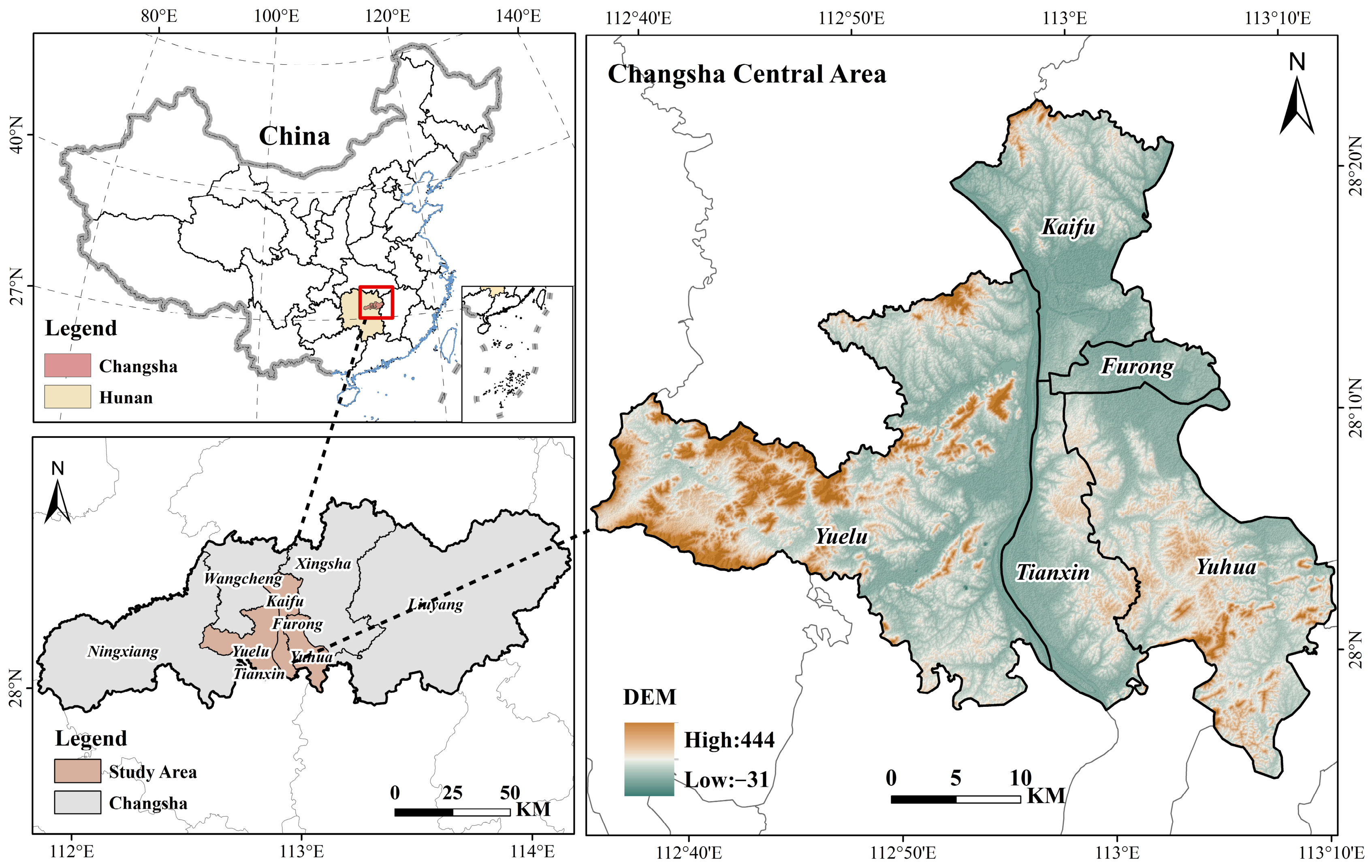
Figure 2. Location of the study area in Changsha, China.
Systems 14 00842 g002
Figure 5. Spatial distribution map of Economic Vitality.
Systems 14 00842 g005
Figure 6. Spatial distribution map of Cultural vitality.
Systems 14 00842 g006
Figure 7. Spatial distribution map of Ecological Vitality.
Systems 14 00842 g007
Figure 8. Spatial Autocorrelation Analysis Map.
Systems 14 00842 g008
Figure 9. Performance comparison of six machine learning models on the test set.
Systems 14 00842 g009
Figure 10. Boxplot distribution of evaluation metrics across different models.
Systems 14 00842 g010
Figure 11. Composite plot of SHAP contributions.
Systems 14 00842 g011
Figure 12. Honeycomb Plot of SHAP value.
Systems 14 00842 g012
Figure 17. Objective environment bivariate SHAP dependence plots.
Systems 14 00842 g017
Figure 18. Subjective environment bivariate SHAP dependence plots.
Systems 14 00842 g018
Table 1. Data description for constructing the urban vitality indicator system.
DimensionDate TypeQuantification MethodData SourceLiteratureWeight
Social VitalityBaidu HeatmapAverage Heatmap value across all time periods within the community unitshttps://rq.baidu.com/
(accessed on 30 December 2025)
[12,43,58]0.058
Social Media Check-insNumber of comments and likes within the community unitshttps://weibo.cn/
(accessed on 31 December 2025)
[23,45,59]0.334
Economic VitalityCommercial Service FacilitiesNumber of POIs for dining, shopping, entertainment, accommodation, etc., within the community unitshttps://ditu.amap.com/
(accessed on 30 July 2025)
[54,60]0.094
Consumption ReviewsNumber of reviews for dining, shopping, entertainment, accommodation, sports, etc., within the community unitshttps://www.dianping.com/
(accessed on 29 December 2025)
[12,61]0.174
Nighttime Light IntensityAverage value of NPP/VIIRS nighttime light pixels within the community unitshttps://search.earthdata.nasa.gov/
(accessed on 29 December 2025)
[27,43,60]0.045
Cultural VitalityCultural Facility DensityNumber of POIs for museums, libraries, art galleries, theaters, cultural centers, exhibition halls, media institutions, bookstores, cultural/creative shops, etc.https://ditu.amap.com/
(accessed on 30 July 2025)
[27,40,60]0.084
Public Service Facility DensityNumber of POIs for schools, research institutions, training centers, sports/leisure, medical/health care, etc., within the community unitshttps://ditu.amap.com/
(accessed on 30 July 2025)
[54,60]0.096
Ecological VitalityLandscape Facility
Density
Number of POIs for scenic spots, parks, squares, etc., within the community unitshttps://ditu.amap.com/
(accessed on 30 July 2025)
[54,62]0.105
Vegetation Coverage IndexAverage Normalized Difference Vegetation Index (NDVI) within the community unitshttps://search.earthdata.nasa.gov/
(accessed on 29 December 2025)
[11,15,57]0.009
Table 2. Parameter tuning methods and ranges for the XGBoost model.
HyperparameterSearch MethodSearch RangeOptimal Value
learning-rateLog-uniform1 × 10−3–0.90.0329
max-depthInteger2–53
reg-lambdaLog-uniform1 × 10−4–1000.0002
gammaLog-uniform1 × 10−4–1000.0003
min-child-samplesInteger2–106
n-estimatorsInteger1–500108
colsample-bytreeLog-uniform0.1–10.1507
subsampleLog-uniform0.1–10.1928
random-stateFixed11
n-jobsFixed−1−1
Table 3. Construction of the index system for factors influencing the urban vitality.
DimensionVariableMeasuring MethodUnitsLiterature
Objective EnvironmentBuilding DensityBuilding footprint area within the community units m 2 [11,13,18]
Functional Aggregation DegreeDensity of POIs for commerceculture, public services, ecological landscapes, etc., within the community units n / k m 2 [13,23,64]
Functional DiversityDegree of mixture of POIs for commerce, culture, public services, ecological landscapes, etc., within the community units-[2,23,40]
Road Network DensityTotal length of roads within the community unit k m / k m 2 [13,27,43]
Intersection DensityNumber of intersections within the community units n / k m 2 [7,10,27]
PM2.5 DensitySatellite-derived annual average near-surface PM2.5 concentrationμg/m3[43,60]
Population DensityNumber of permanent residents within the community units p e o p l e / k m 2 [13,15]
Housing Price LevelAverage housing price within the community unitsCNY/m2[7,18,43]
Transit Station DensityNumber of bus and subway stations within the community units n / k m 2 [7,17,47]
Spatial Enclosure SenseProportion of the visual field occupied by elements other than the sky in Street View imagery within the community units%[12,17,54]
Interface Richness IndexDegree of mixture calculated based on the area of various elements within the community units%[12,17,18]
Environment Openness IndexProportion of sky pixel area in Street View imagery within the community units%[18,40,47]
Walking ConvenienceRatio of pedestrian space to vehicular space within the community units%[12,17]
Motorization LevelProportion of the visual field occupied by motorized lanes in Street View imagery within the community units%[15,17]
Green Visibility IndexProportion of greenery pixel area in Street View imagery within the community units%[12,40,47]
Blue Visibility IndexProportion of water body pixel area in Street View imagery within the community units%[65,66]
Subjective PerceptionLively PerceptionPerception of environmental vibrancy-[16,20,54]
Wealthy PerceptionPerception of environmental affluence-[16,20,54]
Beautiful PerceptionPerception of environmental aesthetics-[15,16,54]
Safety PerceptionPerception of environmental safety-[15,20,54]
Boring PerceptionPerception of environmental boredom-[15,54,64]
Depressing PerceptionPerception of environmental depression-[15,54,64]
Table 4. Model comparison results based on 5-fold cross-validation.
ModelMetricTrain MeanTrain Std.Test MeanTest Std.Train Mean ± Std.Test Mean ± Std.
XGBoostR20.77500.02530.59670.15530.7750 ± 0.02530.5967 ± 0.1553
RMSE0.03860.00360.05110.01800.0386 ± 0.00360.0511 ± 0.0180
MAE0.02410.00180.03080.00640.0241 ± 0.00180.0308 ± 0.0064
LightGBMR20.75920.02600.59080.14910.7592 ± 0.02600.5908 ± 0.1491
RMSE0.03990.00360.05130.01640.0399 ± 0.00360.0513 ± 0.0164
MAE0.02050.00180.03040.00630.0205 ± 0.00180.0304 ± 0.0063
SVRR20.75040.02840.59430.17840.7504 ± 0.02840.5943 ± 0.1784
RMSE0.04070.00400.05110.01910.0407 ± 0.00400.0511 ± 0.0191
MAE0.01610.00140.02880.00850.0161 ± 0.00140.0288 ± 0.0085
ExtraTreesR20.75980.02660.56200.14520.7598 ± 0.02660.5620 ± 0.1452
RMSE0.03980.00320.05320.01670.0398 ± 0.00320.0532 ± 0.0167
MAE0.02370.00180.03120.00600.0237 ± 0.00180.0312 ± 0.0060
GBDTR20.65930.02260.54440.11920.6593 ± 0.02260.5444 ± 0.1192
RMSE0.04750.00330.05440.01570.0475 ± 0.00330.0544 ± 0.0157
MAE0.03040.00130.03560.00540.0304 ± 0.00130.0356 ± 0.0054
RandomForestR20.77000.02510.56900.13110.7700 ± 0.02510.5690 ± 0.1311
RMSE0.03900.00330.05300.01640.0390 ± 0.00330.0529 ± 0.0164
MAE0.02280.00180.03130.00600.0228 ± 0.00180.0313 ± 0.0060
Table 5. SHAP contribution index and ranking.
VariableMean (|SHAP|)Relative Importance %Rank
Building Density0.0101012.511
Functional Aggregation Degree0.006988.642
Intersection Density0.005576.903
Transit Station Density0.005386.674
Housing Price Level0.005206.445
PM2.5 Density0.004725.846
Lively Perception0.004455.517
Population Density0.004065.028
Walking Convenience0.003854.779
Functional Diversity0.003764.6510
Wealthy Perception0.003574.4311
Spatial Enclosure Sense0.003464.2812
Depressing Perception0.002823.4913
Green Visibility Index0.002372.9414
Interface Richness Index0.002342.9015
Motorization Level0.002062.5416
Environment Openness Index0.002002.4817
Boring Perception0.001892.3418
Blue Visibility Index0.001581.9519
Safety Perception0.001571.9420
Beautiful Perception0.001511.8821
Road Network Density0.001511.8722
Disclaimer/Publisher’s Note: The statements, opinions and data contained in all publications are solely those of the individual author(s) and contributor(s) and not of MDPI and/or the editor(s). MDPI and/or the editor(s) disclaim responsibility for any injury to people or property resulting from any ideas, methods, instructions or products referred to in the content.