Governing Workplace Heat Risk Under Climate Change: A Tripartite Evolutionary Game of Regulators, Employers, and Workers

Abstract

Workplace heat exposure under climate change is not only a physical hazard but also a recurrent governance problem involving regulators, employers, and workers. This paper develops a tripartite evolutionary game to examine how workplace heat-risk governance evolves through the interaction of strict regulation, employer prevention investment, and worker symptom reporting. Normal-form Nash and Stackelberg benchmarks are used to clarify the static and sequential counterparts of the evolutionary stability conditions. Heat-risk intensity is introduced as an environmental state that affects accident probability, expected losses, governance costs, and institutional benefits. The model identifies a heat-dependent cooperative stability region: full cooperation is locally stable only when digital monitoring, enforcement incentives, employer investment support, and worker reporting protection jointly satisfy threshold conditions. Extended payoff specifications allow monitoring and regulatory strictness to directly affect worker reporting incentives and link government payoffs to accident-risk reduction. The results show that monitoring and reporting protection may be partially substitutable in the worker-reporting channel but remain non-equivalent at the system level. Long-horizon, shock-recovery, and industry-specific diagnostics further show that isolated instruments often generate partial-governance regimes rather than system-wide cooperation. The findings frame workplace heat adaptation as a complex adaptive governance problem requiring coordinated technological visibility, credible enforcement, employer incentives, and protected worker reporting.

1. Introduction

Climate change is increasing the frequency and severity of workplace heat exposure. Heat stress raises the risk of fatigue, dehydration, reduced concentration, heat-related illness, and occupational injury, particularly in outdoor and physically demanding sectors such as construction, agriculture, logistics, manufacturing, and emergency services. A growing body of empirical research documents the adverse effects of heat exposure on occupational safety and worker health [1,2,3,4]. However, identifying heat exposure as a hazard does not by itself explain how workplaces can govern this risk effectively. Heat-risk prevention depends on whether multiple actors can coordinate their behavior before heat illness becomes severe.

Workplace heat-risk governance is a system-level problem. Governments can introduce heatstroke-prevention rules, conduct inspections, impose penalties, and support preventive investment, but strict enforcement requires administrative capacity and sustained regulatory commitment. Employers can invest in cooling equipment, work-rest arrangements, reporting systems, training, and emergency-response procedures, but these measures impose costs and may be underprovided when enforcement is weak. Workers can report heat-related symptoms or stop work before illness worsens, but reporting may involve income loss, workplace pressure, reputational concerns, or fear of retaliation. These interdependencies create feedback loops: worker reporting improves information available to regulators and employers, monitoring affects the probability that non-compliance is detected, and employer investment changes the health consequences of worker reporting. Workplace heat-risk prevention is therefore not only a technical problem of measuring heat exposure; it is a dynamic governance problem involving strategic interaction among regulators, employers, and workers.

Japan provides a timely institutional context for this problem. In 2025, Japan strengthened workplace heatstroke-prevention requirements through reforms emphasizing early detection, internal reporting systems, emergency-response procedures, and employer preparedness [5]. The revised framework links workplace heat exposure to concrete employer obligations and highlights the importance of reporting channels for suspected heat illness. This institutional development illustrates a broader governance challenge. Even when heat exposure is observable, prevention may fail if employers do not invest in protective systems or if workers do not report symptoms early enough for response procedures to operate. Effective heat-risk governance requires a system in which monitoring, enforcement, employer preparedness, and worker reporting reinforce one another.

This study asks: under what conditions can workplace heat-risk governance evolve toward stable cooperation among government regulators, employers, and workers? To answer this question, I develop a tripartite evolutionary game model in which the government chooses between strict and lenient regulation, employers choose between proactive investment and passive compliance, and workers choose between reporting heat-related symptoms and continuing work. The model introduces heat-risk intensity as an exogenous environmental state that affects accident probability, accident-related losses, regulatory benefits, and governance costs. It also incorporates policy instruments central to workplace heat-risk governance: penalties, subsidies, digital monitoring, detection probability, and worker reporting protection.

The model treats workplace heat-risk governance as a complex adaptive system. The state variables describe the evolving proportions of government regulators adopting strict regulation, employers adopting proactive investment, and workers choosing symptom reporting. The replicator dynamic framework captures boundedly rational adjustment: strategies that yield higher relative payoffs become more prevalent over time. This approach is useful because workplace safety governance is rarely a one-shot decision. Regulators, firms, and workers repeatedly observe costs, risks, enforcement, and responses, and their strategies evolve through adaptation, learning, and institutional feedback.

The analysis produces four main results. First, heat-risk governance is governed by a cooperative stability region rather than by a single equilibrium condition. The monitoring threshold $M_G^{*}\left(\theta \right)$ provides a closed-form boundary showing how environmental heat intensity changes the institutional feasibility of strict regulation. Second, isolated policy instruments generate incomplete governance regimes: penalties can induce regulation without employer investment, while reporting protection can generate worker voice without system-wide prevention. Third, digital monitoring and worker reporting protection stabilize different feedback channels. Monitoring improves visibility and enforcement capacity, whereas reporting protection sustains information flow from workers to the governance system. Fourth, under mild heat-risk intensity, the combined policy package does not converge to full cooperation. In the pure continuous-time replicator system, this appears as neutral boundary cycles around a reporting-face mixed equilibrium; under a weak mutation perturbation, the non-hyperbolic center is destroyed and the system converges to a nearby partial-cooperation regime. The robust conclusion is therefore not the exact closed-orbit geometry, but the failure of mild-heat governance to reach full cooperation outside the cooperative stability region.

This study contributes to the literature in three ways. First, it introduces an explicit environment–institution coupling into occupational safety evolutionary games. Heat-risk intensity enters the accident probability, expected losses, institutional benefits, and governance costs, allowing the paper to derive a heat-dependent cooperative stability boundary. Second, it goes beyond the usual local-stability analysis common in tripartite evolutionary-game studies by combining normal-form Nash and Stackelberg benchmark analyses, threshold analysis, boundary mixed-equilibrium analysis, numerical-scheme checks, perturbation diagnostics, and finite-horizon regime diagnostics. Third, it clarifies the systemic roles of digital monitoring and protected worker reporting. These instruments are not perfect system-level substitutes. In the benchmark model, digital monitoring supports the visibility–enforcement channel, whereas reporting protection supports the reporting–trust channel. An extended worker-payoff specification further allows monitoring and regulatory strictness to directly encourage reporting, showing that the instruments may be partially substitutable in the worker-reporting channel while remaining institutionally distinct at the system level.

These findings imply that workplace heat-risk adaptation should be designed as a coupled governance system rather than as a collection of separate interventions. Penalties, subsidies, monitoring technologies, and worker protection each address different parts of the system. Digital monitoring can make risks and non-compliance more visible, but it must be connected to enforcement and employer obligations. Worker reporting protection can support symptom disclosure, but it must be embedded in credible reporting and emergency-response procedures. Stable workplace heat-risk governance requires technological visibility, enforcement credibility, employer investment incentives, and protected worker voice to operate together.

2. Literature Review

2.1. Heat Exposure, Labor Risk, and Climate Adaptation

This study first relates to the large literature on the economic and health consequences of heat exposure. A central finding in climate economics is that temperature affects human welfare through nonlinear and sector-specific channels. Dell et al. [6] show that temperature shocks reduce economic growth, especially in poorer countries, while Burke et al. [7] document a global nonlinear relationship between temperature and aggregate economic production. Health-based studies in economics further show that temperature extremes increase mortality risk and that adaptation can substantially alter the temperature–health relationship [8,9,10]. At the labor-market level, Graff Zivin and Neidell [11] show that high temperatures reduce labor supply in climate-exposed industries. These studies establish that heat is not only an environmental condition but also an economic constraint that affects productivity, health, and adaptation incentives.

A related public-health and occupational-health literature examines the mechanisms through which heat exposure affects workers. Ebi et al. [12] review the broader health risks of heat extremes and note that high heat stress can reduce physical work capacity and cognitive-motor performance. Flouris et al. [13] provide systematic evidence that occupational heat strain is associated with adverse health and productivity outcomes. More specifically, Binazzi et al. [1] and Fatima et al. [2] synthesize epidemiological evidence linking heat exposure to occupational injuries, while Marinaccio et al. [3] and Gariazzo et al. [4] provide large-scale evidence on sector-specific occupational injury risks under extreme temperature exposure. In the Japanese context, Fu and Sasaki [14] provide prefecture-level evidence that exposure to temperature extremes significantly increases work-related injuries and associated social costs, while workers show limited defensive adjustment through reduced working hours or labor-force exit.

Taken together, this literature motivates the present model in two ways. First, it shows that workplace heat exposure generates real accident, health, and productivity risks. Second, it suggests that individual adaptation alone may be insufficient when prevention requires coordinated action by regulators, firms, and workers. However, this empirical literature primarily estimates the consequences of heat exposure. It does not model the governance mechanism through which enforcement, employer investment, monitoring, and worker reporting jointly determine whether heat-risk prevention becomes self-sustaining.

2.2. Governance, Enforcement, and Information in Risk Regulation

The second body of work concerns enforcement, incentives, and information in governance systems. The economic theory of deterrence begins from the insight that compliance depends jointly on the probability of detection and the magnitude of sanctions [15]. Principal–agent theory further shows that monitoring and observability affect incentives when actions are costly or imperfectly observed [16]. These ideas are directly relevant to workplace heat-risk governance: employers may underinvest in prevention when violations are difficult to detect, while regulators face costs in maintaining inspection and monitoring capacity.

Workplace heat-risk governance also resembles a collective-action problem. Prevention depends on the interaction of multiple actors rather than on a single optimizing decision-maker. Ostrom [17] emphasizes that social-ecological systems should be analyzed through the interaction between resource systems, governance systems, users, and outcomes. Although the present setting concerns occupational safety rather than natural-resource management, the systems logic is similar: environmental pressure interacts with institutional rules, information flows, and actor incentives. Heat-risk governance therefore requires more than identifying the physical hazard. It requires a rule system in which monitoring, enforcement, employer preparedness, and worker reporting reinforce one another.

Worker reporting is especially important because heat illness prevention depends on early information. In organizational research, Hirschman [18] conceptualizes voice as a response to organizational decline, while Edmondson [19] shows that psychological safety affects whether members of a team speak up and learn from errors. Applied to heat-risk governance, worker reporting can be understood as an information channel that allows early detection and response. However, reporting is costly when workers face income loss, stigma, or retaliation. This explains why reporting protection is modeled as a distinct institutional instrument rather than as a by-product of monitoring technology.

2.3. Evolutionary Games, Cooperation, and Adaptive Governance

The third body of work provides the dynamic foundation for the model. Evolutionary game theory was introduced to study how strategies spread when agents adapt through selection, imitation, and payoff comparison rather than through one-shot perfect rationality. Maynard Smith and Price [20] introduced the evolutionary-stability approach, and Taylor and Jonker [21] formalized game dynamics through the replicator equation. Later treatments by Weibull [22], Fudenberg and Levine [23], Hofbauer and Sigmund [24], and Sandholm [25] developed evolutionary and learning foundations for strategic adjustment in populations.

This framework is useful for workplace safety governance because regulators, employers, and workers do not choose strategies only once. They repeatedly observe inspection outcomes, accident losses, compliance costs, reporting consequences, and institutional responses. Strategies that perform better under a given institutional environment become more prevalent, while poorly performing strategies decline. The replicator dynamic therefore provides a parsimonious way to represent boundedly rational adjustment in a coupled governance system.

Recent applied studies have used tripartite evolutionary games to examine multi-actor governance problems in environmental regulation, public participation, and safety supervision. In environmental governance, Zhou et al. [26] analyze pollution-control strategies under government regulation, while Zhu et al. [27] model the strategic interaction among enterprises, local governments, and the central government under central-government intervention. Wei et al. [28] examine third-party environmental pollution management involving pollution-control firms, professional environmental testing institutions, and government regulators. Public participation has also been incorporated into multi-player environmental governance models. For example, Chu et al. [29] study how public participation can improve environmental governance, and Wang et al. [30] analyze collaborative air-pollution control among enterprises, the public, and government. More recent systems-oriented applications introduce stochastic disturbances and uncertainty into tripartite governance dynamics [31]. In safety-related settings, Pi et al. [32] examine construction safety performance through an evolutionary-game framework, Guo et al. [33] analyze the promotion of construction safety education, and Jiang et al. [34] model construction safety supervision among government supervision agencies, general contractors, and supervision engineers. These studies show that tripartite evolutionary games have become a standard tool for analyzing regulatory incentives, compliance behavior, and multi-actor governance in environmental and safety domains.

The present study builds on this applied literature but differs from it in three respects. First, it introduces heat-risk intensity $\left(\theta \right)$ as an explicit environmental state that shifts accident probability, expected losses, institutional benefits, and governance costs, thereby generating a heat-dependent stability threshold $\left(M_G^{*}\left(\theta \right)\right)$. Second, it treats non-hyperbolic boundary mixed equilibria explicitly rather than relying only on pure-strategy local stability and terminal simulation outcomes; the analysis combines boundary-equilibrium characterization, numerical-scheme checks, perturbation diagnostics, and finite-horizon regime diagnostics. Third, it separates digital monitoring and worker reporting protection as two distinct governance channels. Digital monitoring strengthens the visibility–enforcement feedback loop, whereas reporting protection strengthens the reporting–trust feedback loop. This distinction is particularly important for workplace heat-risk governance because technological detectability and worker willingness to report symptoms are not institutionally equivalent.

2.4. Positioning of This Study

The existing literature establishes four important points. First, heat exposure creates substantial health, productivity, and injury risks. Second, economic and public-health studies show that adaptation matters, but they usually treat adaptation as an outcome rather than as a strategic governance process. Third, enforcement and information are central to compliance when prevention is costly and actions are imperfectly observed. Fourth, evolutionary game theory provides a dynamic framework for studying how boundedly rational actors adapt in repeated strategic environments.

The present study connects these strands by modeling workplace heat-risk governance as a tripartite adaptive system. Unlike the empirical heat-risk literature, it does not estimate the reduced-form effect of temperature on injuries. Instead, it explains why heat-risk prevention may fail even when the hazard is recognized. Unlike standard enforcement models, it explicitly includes workers as strategic information providers whose reporting decision depends on institutional protection. Unlike many applied tripartite evolutionary-game studies of environmental regulation and safety supervision, it introduces heat-risk intensity as an environmental state that changes accident probability, expected losses, regulatory salience, and governance costs. This environment–institution coupling yields a heat-dependent cooperative stability boundary, represented most clearly by the monitoring threshold $\left(M_G^{*}\left(\theta \right)\right)$. The paper also gives explicit attention to non-hyperbolic boundary mixed equilibria, numerical-scheme sensitivity, and perturbation robustness, rather than treating all simulation endpoints as asymptotically stable outcomes. The contribution is therefore to characterize the cooperative stability region of a climate-induced occupational safety system and to show how technological visibility, credible enforcement, employer investment support, and protected worker reporting jointly determine whether full cooperation is locally attainable.

This positioning clarifies the specific research gap addressed by the paper. Existing heat-exposure studies establish the existence of occupational risk but do not model the strategic governance mechanism. Existing enforcement and monitoring theories explain compliance incentives but usually do not include climate-induced heat intensity as an environmental state variable. Existing tripartite evolutionary-game studies analyze multi-actor governance, but they rarely combine heat-risk intensity, worker symptom reporting, digital monitoring, and perturbation-sensitive boundary dynamics in one occupational safety framework. The present study is designed to fill this intersection rather than to provide a reduced-form empirical estimate of heat effects.

3. Institutional and Conceptual Framework

Workplace heat-risk governance involves several interdependent tasks: monitoring heat exposure, reducing exposure through engineering and administrative controls, training workers, establishing reporting channels, providing rest and cooling measures, and responding quickly to suspected heat illness. These measures require coordination among public regulators, employers, supervisors, and workers.

Each actor faces different incentives. Government agencies seek to reduce occupational health risks and maintain regulatory legitimacy, but strict enforcement requires administrative resources. Employers may benefit from preventing accidents and maintaining productivity, but proactive investment requires upfront costs. Workers benefit from reporting symptoms and avoiding heat illness, but reporting may involve opportunity costs, workplace pressure, reputational concerns, or fear of retaliation. These conflicting incentives create a strategic governance problem. The purpose of this section is to clarify how this governance problem is institutionally grounded and how it is translated into the tripartite evolutionary-game framework.

3.1. Institutional Background: Japan’s 2025 Workplace Heatstroke-Prevention Reform

Japan provides a timely institutional context for analyzing workplace heat-risk governance. In response to the growing severity of occupational heatstroke cases, the Ministry of Health, Labour and Welfare strengthened workplace heatstroke-prevention measures through the revision of the Ordinance on Industrial Safety and Health. The revised rule came into effect on 1 June 2025, with the central objective of preventing the aggravation of heatstroke by improving early detection, reporting, and emergency response procedures in workplaces [5].

The strengthened rule is particularly relevant to this study because it explicitly emphasizes organizational reporting and response systems. Employers are required to establish a reporting system in advance so that workers with subjective symptoms of heatstroke, or persons who identify workers suspected of heatstroke, can report such cases to designated persons or contact points within the workplace. Employers are also required to inform relevant workers of this reporting system. In addition, employers must prepare procedures for responding to suspected heatstroke cases, including removing affected workers from work, cooling the body, transporting workers to medical institutions when necessary, and establishing emergency communication procedures.

The scope of the revised rule is defined by heat exposure and work duration. The measures apply to work that is expected to be conducted in a hot environment where the wet-bulb globe temperature (WBGT) is $28°\mathrm{C}$ or higher, or where the air temperature is $31°\mathrm{C}$ or higher, and where work is expected to continue for one hour or more, or for more than four hours per day [5]. This regulatory threshold directly links workplace heat exposure to employer obligations.

Although the model is motivated by Japan’s 2025 reform, the underlying policy logic is not Japan-specific. Internationally, workplace heat-risk assessment commonly relies on WBGT-based heat-stress evaluation. The ISO 7243 standard [35] provides a widely used WBGT-based framework for assessing heat stress in hot environments, while the National Institute for Occupational Safety and Health (NIOSH) criteria document on occupational exposure to heat and hot environments emphasizes heat-stress management, acclimatization, training, hydration, work-rest arrangements, and medical monitoring [36,37]. These international standards reinforce the broader relevance of modeling workplace heat-risk governance as a system that combines exposure monitoring, employer preparedness, worker reporting, and emergency response.

Japan’s institutional reform is important for the present model for three reasons. First, it shifts workplace heatstroke prevention from a general occupational health recommendation toward a more concrete compliance requirement. This justifies modeling the government as a strategic regulator choosing between strict and lenient enforcement. Second, the reform makes employer preparedness central to heat-risk governance. Employers must not only recognize heat risk but also establish reporting systems, cooling and rest measures, training, and emergency-response procedures, which correspond to proactive investment in the model. Third, the reform explicitly highlights worker reporting as a key mechanism for preventing severe heatstroke outcomes. This justifies modeling workers as strategic actors who choose between reporting symptoms and continuing work.

In the model, strict government regulation is represented by x, employer investment in reporting systems, cooling measures, training, and emergency procedures is represented by y, and worker reporting of heat-related symptoms is represented by z. The penalty parameter F captures the cost of being detected as non-compliant, the subsidy parameter $S_b$ captures policy support for employer prevention investment, the reporting protection parameter $P_W$ captures institutional protection for workers who report symptoms, and the digital monitoring parameter M captures the use of WBGT monitoring, wearable devices, digital inspection systems, and artificial intelligence (AI)-enabled heat-warning systems to improve detection and reduce governance costs.

3.2. Basic Assumptions

Assumption 1 

(Bounded rationality and adaptive adjustment). Government regulators, employers, and workers are boundedly rational actors. They do not solve a one-shot full-information optimization problem. Instead, their strategies evolve through repeated adjustment, learning, imitation, and feedback from regulatory outcomes, workplace costs, and health risks.

Assumption 2 

(Strategy sets). The government chooses between strict regulation and lenient regulation. Employers choose between proactive investment in workplace heat-risk prevention and passive compliance. Workers choose between reporting heat-related symptoms or stopping work and continuing work without reporting.

Assumption 3 

(Heat-risk intensity). Heat-risk intensity $\theta \in [0,1]$ is an exogenous environmental state. It affects the baseline accident probability, accident-related losses, regulatory benefits, and governance costs, but it is not itself a strategic actor.

Assumption 4 

(Benchmark distinction between monitoring and protection). In the benchmark specification, digital monitoring M and worker reporting protection $P_W$ perform different functions in the governance system. Digital monitoring creates technological visibility by raising detection probability and lowering governance costs. Worker reporting protection creates institutional trust by reducing the private cost and perceived risk of reporting symptoms. This benchmark distinction is later relaxed by an extended worker-payoff specification in which monitoring and regulatory strictness can also directly influence reporting incentives.

3.3. Policy Design Layer and Evolutionary Interaction Layer

The model separates policy design from evolutionary interaction. The policy design layer consists of parameters chosen or enabled by the institutional environment before the evolutionary process unfolds. These include the penalty intensity F, the employer subsidy $S_b$, digital monitoring capacity M, and worker reporting protection $P_W$. Comparative-static and scenario analyses vary these parameters to represent alternative policy designs.

The evolutionary interaction layer consists of the state variables x, y, and z. Given a policy design, government regulators adapt between strict and lenient regulation, employers adapt between proactive investment and passive compliance, and workers adapt between symptom reporting and continuing work. Strict regulation activates the penalty and subsidy instruments in the payoff structure: passive employers face expected penalties, whereas proactive employers receive policy support. Digital monitoring is treated as a pre-existing monitoring capacity or infrastructure level that increases detection probability and reduces regulatory and investment costs. The model does not separately optimize the public budget for installing monitoring infrastructure; instead, M is used as a policy-design parameter whose system effects are examined through comparative statics and finite-horizon diagnostics.

In the Japanese institutional setting, this two-layer interpretation can be mapped onto the division between national policy design and decentralized enforcement. The Ministry of Health, Labour and Welfare sets the regulatory framework and defines the institutional parameters of heatstroke-prevention governance, including employer obligations, reporting-system requirements, emergency-response procedures, and sanctioning rules. By contrast, prefectural labour bureaus and Labour Standards Inspection Offices implement inspection and enforcement in practice. The government population in the evolutionary layer should therefore be interpreted as decentralized enforcement units or regulatory actors whose strictness may vary with administrative capacity, monitoring infrastructure, perceived heat-risk salience, and enforcement costs.

This institutional mapping resolves the apparent tension between the government as a policy designer setting $(F,S_b,M,P_W)$ and the government as an adaptive enforcement population choosing between strict and lenient regulation. A policy designer first sets the institutional environment. The tripartite system then evolves under the induced payoff structure. Policy simulations therefore compare different institutional designs rather than treating all policy tools as simultaneous strategic choices by the government population.

3.4. Notation and Institutional Mapping

Table 1. Notation and definitions.

Symbol	Definition	Governance Interpretation
x	Share choosing strict regulation	Regulatory enforcement intensity
y	Share choosing proactive investment	Employer prevention and emergency preparedness
z	Share choosing symptom reporting	Protected worker voice and early detection
$\theta$	Heat-risk intensity	Climate-induced heat exposure
M	Digital monitoring	wet-bulb globe temperature (WBGT) monitoring, wearables, digital inspection, artificial intelligence (AI) warnings
F	Penalty intensity	Cost of detected non-compliance
$S_b$	Employer subsidy	Public support for prevention investment
$P_W$	Worker reporting protection	Institutional protection for symptom disclosure
${\psi }_M$	Direct monitoring effect on reporting	Extended-specification reporting incentive from monitoring evidence
${\psi }_x$	Direct regulatory effect on reporting	Extended-specification reporting incentive from regulatory credibility
$p_0\left(\theta \right)$	Baseline accident probability	Heat-related accident risk without investment/reporting
$q(M,z)$	Detection probability	Visibility generated by monitoring and worker reports
$B_G\left(\theta \right)$	Institutional benefit of strict regulation	Legitimacy and credibility from regulatory action
$A\left(\theta \right)$	Governance-failure loss	Political/social loss from failed prevention
$C_G(M,\theta )$	Regulatory cost	Administrative burden of strict enforcement
$C_I(M,\theta )$	Investment cost	Employer cost of prevention systems
$L_E\left(\theta \right)$	Employer accident loss	Compensation, disruption, reputation, and productivity losses
$H\left(\theta \right)$	Worker health loss	Expected health damage from heat exposure
$R_E$	Employer reputation benefit	Private return to proactive prevention
K	Safety-culture benefit for workers	Reporting benefit when employers invest
$C_R$	Worker reporting cost	Income, time, pressure, or retaliation cost of reporting

defines the main variables and parameters used in the model, while

Table 2. Mapping between workplace heatstroke-prevention governance and model components.

Governance Component	Institutional Meaning	Model Representation
Heat exposure threshold	wet-bulb globe temperature (WBGT)/air-temperature threshold and work duration	$\theta$, $p_0\left(\theta \right)$
Government inspection	Strict enforcement and sanctioning capacity	x, F, $C_G(M,\theta )$
Employer preparedness	Reporting systems, cooling measures, training, emergency response	y, $C_I(M,\theta )$, $S_b$
Worker symptom reporting	Early disclosure of suspected heat illness	z, $P_W$, $C_R$
Digital heat monitoring	WBGT sensors, wearables, AI-enabled warning systems	M, $q(M,z)$
Accident prevention	Reduced heat-related accident probability	$p(y,z;\theta )$
Governance failure	Failure to prevent severe heat illness	$A\left(\theta \right)$, $L_E\left(\theta \right)$, $H\left(\theta \right)$

maps these model components to the institutional elements of workplace heatstroke-prevention governance.

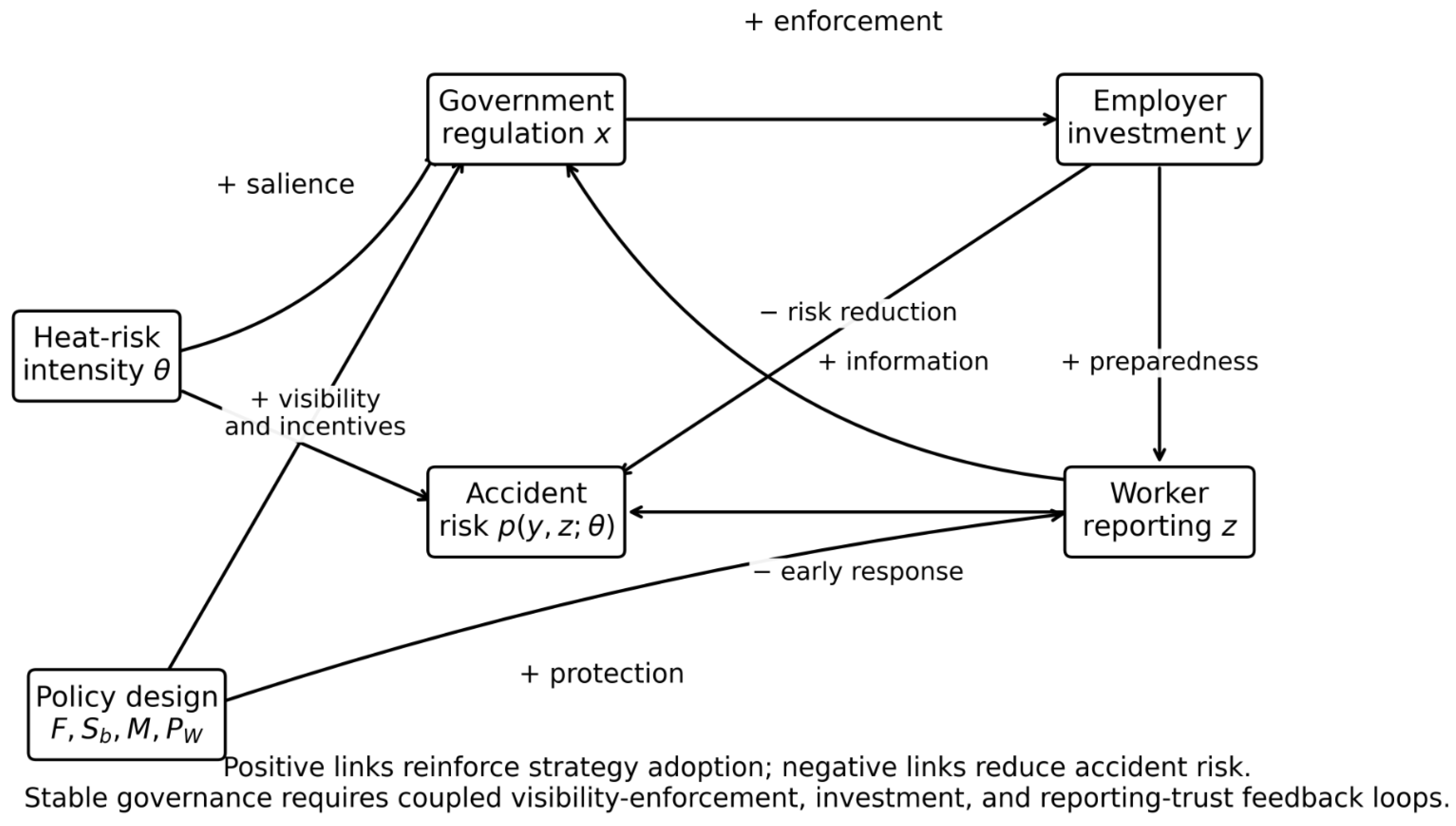
Figure 1 summarizes the causal feedback structure of workplace heat-risk governance and highlights the visibility–enforcement, enforcement–investment, and reporting–trust channels.

The figure summarizes the core feedback architecture. Heat-risk intensity raises baseline accident pressure and regulatory salience. Digital monitoring strengthens the visibility–enforcement channel by increasing detectability and reducing governance costs. Employer investment and worker reporting reduce accident risk, while worker reporting also improves information flow to the governance system. These feedback loops are coupled: visibility without worker trust may not generate reports, and reporting without enforcement may not generate employer investment. The framework therefore treats workplace heat-risk governance as a coupled adaptive system rather than as a single-actor compliance problem.

4. Materials and Methods: Model Setup

4.1. Players, Strategies, and Heat-Risk Intensity

This study considers a tripartite evolutionary game among the government, employers, and workers. The government chooses between strict regulation S and lenient regulation L. Employers choose between proactive investment I in workplace heat-risk prevention and passive compliance P. Workers choose between reporting heat-related symptoms or stopping work R and continuing work C.

Let $x\in [0,1]$ denote the proportion of government regulators adopting strict regulation, $y\in [0,1]$ denote the proportion of employers adopting proactive investment, and $z\in [0,1]$ denote the proportion of workers choosing symptom reporting.

To explicitly capture the role of climate-induced heat exposure, the model introduces an exogenous heat-risk intensity parameter $\theta \in [0,1]$. A higher value of $\theta$ represents more severe workplace heat exposure, such as more days exceeding regulatory heat thresholds, higher WBGT, or more intense heatwaves. Temperature is treated as an exogenous environmental state rather than a strategic actor. It affects the evolutionary system by changing accident probabilities, accident-related losses, and the costs and benefits of governance.

4.2. Heat-Related Accident Risk

Let $p_0\left(\theta \right)$ denote the baseline probability of heat-related accidents when employers do not invest and workers do not report. The baseline accident probability is increasing in heat-risk intensity:

$$p_0^{\prime }\left(\theta \right)>0.$$

For numerical simulations, the baseline accident probability is specified as:

$$p_0\left(\theta \right)=p_{00}+{\gamma }_p\theta .$$

(1)

where $p_{00}>0$ and ${\gamma }_p>0$. The value of $p_0\left(\theta \right)$ is assumed to lie in $(0,1)$.

Employer investment reduces accident risk by proportion $a\in (0,1)$, while worker reporting reduces accident risk by proportion $b\in (0,1)$. Therefore, the heat-related accident probability is:

$$p(y,z;\theta )=p_0\left(\theta \right)(1-ay)(1-bz).$$

(2)

The parameter b should be interpreted as the reduction in the probability of severe heat-related outcomes due to early reporting and response, rather than as a reduction in physical heat exposure itself. For the pure strategy combinations:

$$p_{IR}\left(\theta \right)=p_0\left(\theta \right)(1-a)(1-b),p_{IC}\left(\theta \right)=p_0\left(\theta \right)(1-a),$$

$$p_{PR}\left(\theta \right)=p_0\left(\theta \right)(1-b),p_{PC}\left(\theta \right)=p_0\left(\theta \right).$$

4.3. Digital Monitoring and Temperature-Dependent Costs

Digital monitoring, denoted by $M\in [0,1]$, includes WBGT monitoring, wearable devices, digital inspection systems, and AI-enabled heat-warning systems. It increases the probability that passive employer compliance is detected:

$$q(M,z)=q_0+\alpha M+\lambda z.$$

(3)

where $q_0$ is the baseline detection probability, $\alpha >0$ captures the effect of digital monitoring, and $\lambda >0$ captures the informational contribution of worker reporting. The benchmark parameter range satisfies $q_0+\alpha M+\lambda z<1$. In the baseline simulations, $q_0+\alpha M+\lambda =0.60<1$, so the Jacobian analysis and numerical simulations do not require truncating the detection function.

Heat-risk intensity also affects governance costs and expected losses. Let

$$B_G\left(\theta \right)=B_{G0}+{\beta }_G\theta$$

be the institutional benefit of strict regulation, and 

$$A\left(\theta \right)=A_0+{\beta }_A\theta$$

be the social or political loss when governance fails. Similarly, the employer accident loss and worker health loss are:

$$L_E\left(\theta \right)=L_{E0}+{\beta }_E\theta ,H\left(\theta \right)=H_0+{\beta }_H\theta .$$

The costs of strict regulation and proactive investment are:

$$C_G(M,\theta )=C_{G0}-\mu M+{\chi }_G\theta ,$$

$$C_I(M,\theta )=C_{I0}-\eta M+{\chi }_I\theta .$$

Thus, digital monitoring reduces governance and investment costs, while stronger heat shocks may increase the administrative and operational burden of heat-risk prevention. The employer reputation benefit $R_E$ is kept constant in the benchmark model to isolate the effect of heat risk on accident losses and governance salience; allowing $R_E$ to increase with $\theta$ would further strengthen employer incentives to invest and is therefore conservative relative to the main mechanism.

A remark on modeling scope is warranted. In the benchmark specification, the detection probability $q(M,z)$ does not enter the worker’s payoff difference ${\Delta }_W$ directly. This benchmark separation allows the model to distinguish two governance channels: digital monitoring M creates technological visibility by increasing detection probability and reducing governance and investment costs, whereas worker reporting protection $P_W$ creates institutional trust by directly reducing the private cost and perceived risk of reporting symptoms. This separation is useful for identifying the baseline visibility–enforcement and reporting–trust mechanisms. However, monitoring technology and regulatory strictness may also affect worker reporting incentives in practice, for example by providing objective evidence, making heat risk more visible, or increasing confidence that reports will be acted upon. Section 7.6 therefore relaxes the benchmark assumption and introduces an extended worker-payoff specification in which digital monitoring and regulatory intensity directly affect worker reporting incentives.

4.4. Pure-Strategy Payoff Matrix

The expected payoff differences used below are derived from the pure-strategy payoff matrix in

Table 3. Pure-strategy payoff matrix for the tripartite heat-risk governance game.

Strategy Profile	Government Payoff	Employer Payoff	Worker Payoff
$(S,I,R)$	$B-C_G-S_b$	$R_E+S_b-C_I-Lp(1-a)(1-b)$	$P_W+K-C_R-Hp(1-a)(1-b)$
$(S,I,C)$	$B-C_G-S_b$	$R_E+S_b-C_I-Lp(1-a)$	$-Hp(1-a)$
$(S,P,R)$	$B-C_G+q_1^{M}F$	$-q_1^{M}F-Lp(1-b)$	$P_W-C_R-Hp(1-b)$
$(S,P,C)$	$B-C_G+q_0^{M}F$	$-q_0^{M}F-Lp$	$-Hp$
$(L,I,R)$	0	$R_E-C_I-Lp(1-a)(1-b)$	$P_W+K-C_R-Hp(1-a)(1-b)$
$(L,I,C)$	0	$R_E-C_I-Lp(1-a)$	$-Hp(1-a)$
$(L,P,R)$	0	$-Lp(1-b)$	$P_W-C_R-Hp(1-b)$
$(L,P,C)$	$-A$	$-Lp$	$-Hp$

. Let $B=B_G\left(\theta \right)$, $A=A\left(\theta \right)$, $C_G=C_G(M,\theta )$, $C_I=C_I(M,\theta )$, $L=L_E\left(\theta \right)$, $H=H\left(\theta \right)$, $p=p_0\left(\theta \right)$, $q_0^M=q_0+\alpha M$, and $q_1^M=q_0+\alpha M+\lambda$. The strict-regulation payoff includes the subsidy cost only when employers invest and includes expected penalties only when employers remain passive. Under lenient regulation, the government is normalized to receive zero unless both employers are passive and workers do not report, in which case governance failure creates the loss $-A$. This normalization makes the cost of leniency state-dependent while keeping the payoff comparison focused on the institutional consequences of failed prevention.

The matrix makes the main asymmetries explicit. First, subsidies are paid only to proactive employers under strict regulation, so the government’s subsidy cost is $-S_b$ in profiles with $(S,I,·)$. Second, penalties are paid only by passive employers when the government regulates strictly, so expected penalty terms appear in $(S,P,R)$ and $(S,P,C)$. Third, lenient-regulation failure costs are normalized to arise in the state $(L,P,C)$, where neither employer investment nor worker reporting mitigates the risk. If either employer investment or worker reporting is present, the normalized governance-failure loss is set to zero in the benchmark specification. This assumption is strong. Section 7.5 provides a quantitative robustness check using a failure-proportional leniency-loss specification, while Section 8.4 discusses the remaining modeling limitations of the benchmark payoff normalization.

4.5. Expected Payoffs

Taking expectations over the population shares in Table 3 gives the strategy-specific expected payoffs. For example, strict regulation yields the institutional benefit and regulatory cost in all employer-worker states, pays subsidies in proportion to employer investment, and receives expected penalties from passive employers.

The expected payoff of strict regulation is:

$$U_G^S=B_G\left(\theta \right)-C_G(M,\theta )-S_{b}y+q(M,z)F(1-y).$$

(4)

The expected payoff of lenient regulation is:

$$U_G^L=-A\left(\theta \right)(1-y)(1-z).$$

(5)

Therefore, the payoff difference between strict and lenient regulation is:

$${\Delta }_G=U_G^S-U_G^L=B_G\left(\theta \right)-C_G(M,\theta )-S_{b}y+q(M,z)F(1-y)+A\left(\theta \right)(1-y)(1-z).$$

(6)

The expected payoff of proactive employer investment is:

$$U_E^I=R_E+x{S}_b-C_I(M,\theta )-L_E\left(\theta \right)p_0\left(\theta \right)(1-a)(1-bz).$$

(7)

The expected payoff of passive compliance is:

$$U_E^P=-xq(M,z)F-L_E\left(\theta \right)p_0\left(\theta \right)(1-bz).$$

(8)

Thus,

$${\Delta }_E=U_E^I-U_E^P=R_E+x{S}_b-C_I(M,\theta )+xq(M,z)F+L_E\left(\theta \right)p_0\left(\theta \right)a(1-bz).$$

(9)

Worker reporting protection is treated as an institutional protection parameter $P_W$. The expected payoff of reporting is:

$$U_W^R=P_W+yK-C_R-H\left(\theta \right)p_0\left(\theta \right)(1-ay)(1-b).$$

(10)

The expected payoff of continuing work is:

$$U_W^C=-H\left(\theta \right)p_0\left(\theta \right)(1-ay).$$

(11)

Therefore,

$${\Delta }_W=U_W^R-U_W^C=P_W+yK-C_R+H\left(\theta \right)p_0\left(\theta \right)b(1-ay).$$

(12)

4.6. Benchmark Game Representations: Nash, Stackelberg, and Evolutionary Dynamics

The payoff matrix in Table 3 can be interpreted in three related ways. First, it defines a three-player normal-form game in which the government, employers, and workers choose their strategies simultaneously. Second, it can be used to construct a sequential benchmark in which the government commits to a regulatory strategy before employers and workers choose their responses. Third, it can be embedded in an evolutionary dynamic system in which population shares adjust gradually according to payoff differences. This comparison follows standard distinctions between static, sequential, and evolutionary representations of strategic interaction [22,24,25,38,39]. This subsection clarifies the relationship among these representations and explains why the continuous-time evolutionary framework is used as the main model of the paper.

4.6.1. Normal-Form Nash Benchmark

Consider first the one-shot normal-form game defined by Table 3. The government chooses between strict regulation S and lenient regulation L, employers choose between proactive investment I and passive compliance P, and workers choose between reporting heat-related symptoms R and continuing work C.

Let

$${\Delta }_G(e,w)=U_G(S,e,w)-U_G(L,e,w),$$

$${\Delta }_E(g,w)=U_E(I,g,w)-U_E(P,g,w),$$

and

$${\Delta }_W(g,e)=U_W(R,g,e)-U_W(C,g,e),$$

where $g\in \{S,L\}$, $e\in \{I,P\}$, and $w\in \{R,C\}$. These payoff differences correspond to the boundary payoff differences defined in Section 5.4. For example, $G_{11}$ is the government’s payoff gain from strict regulation when employers invest and workers report, $E_{11}$ is the employers’ payoff gain from investment when the government regulates strictly and workers report, and $W_1$ is the workers’ payoff gain from reporting when employers invest.

A pure-strategy profile is a Nash equilibrium if no player has a profitable unilateral deviation. Therefore, the eight pure-strategy profiles satisfy the Nash conditions summarized in

Table 4. Pure-strategy Nash equilibrium conditions.

Strategy Profile	Interpretation	Nash Equilibrium Condition
$(L,P,C)$	Non-cooperation	$G_{00}\le 0,E_{00}\le 0,W_0\le 0$
$(L,P,R)$	Reporting only	$G_{01}\le 0,E_{01}\le 0,W_0\ge 0$
$(L,I,C)$	Employer investment only	$G_{10}\le 0,E_{00}\ge 0,W_1\le 0$
$(L,I,R)$	Employer-worker cooperation	$G_{11}\le 0,E_{01}\ge 0,W_1\ge 0$
$(S,P,C)$	Regulation only	$G_{00}\ge 0,E_{10}\le 0,W_0\le 0$
$(S,P,R)$	Regulation and reporting	$G_{01}\ge 0,E_{11}\le 0,W_0\ge 0$
$(S,I,C)$	Regulation and investment	$G_{10}\ge 0,E_{10}\ge 0,W_1\le 0$
$(S,I,R)$	Full cooperation	$G_{11}\ge 0,E_{11}\ge 0,W_1\ge 0$

.

The cooperative profile $(S,I,R)$ is therefore a Nash equilibrium if and only if

$$G_{11}\ge 0,E_{11}\ge 0,W_1\ge 0.$$

It is a strict Nash equilibrium if all three inequalities hold strictly:

$$G_{11}>0,E_{11}>0,W_1>0.$$

This condition is closely related to the local-stability condition of the evolutionary model. This relation between strict Nash incentives and local stability in two-strategy population dynamics is consistent with standard evolutionary-game theory [22,24]. At the cooperative vertex $E_8=(1,1,1)$, the eigenvalues of the replicator system are

$${\lambda }_1=-G_{11},{\lambda }_2=-E_{11},{\lambda }_3=-W_1.$$

Thus, $E_8$ is locally asymptotically stable under the continuous-time replicator dynamics if and only if the cooperative profile $(S,I,R)$ is a strict Nash equilibrium of the underlying normal-form game.

The Nash benchmark therefore provides a static incentive-compatibility interpretation of the evolutionary stability result. However, the Nash analysis does not describe how the system reaches a given equilibrium, whether the cooperative equilibrium is attainable from different initial conditions, or whether non-hyperbolic boundary dynamics arise outside the cooperative stability region. These questions require a dynamic representation.

4.6.2. Stackelberg Benchmark with Government Commitment

A sequential benchmark can also be constructed from the same payoff matrix. In this representation, the government first commits to either strict regulation S or lenient regulation L. Employers and workers observe the government’s regulatory choice and then simultaneously choose between investment and passive compliance, and between reporting and continuing work.

For a given government action $g\in \{S,L\}$, the employers and workers play a two-player follower subgame. Because this follower subgame may admit multiple Nash equilibria, the Stackelberg benchmark is generally set-valued rather than single-valued. Let

$${\mathcal{N}}_{EW}\left(g\right)=\{(e,w):(e,w)\mathrm{is}\mathrm{a}\mathrm{Nash}\mathrm{equilibrium}\mathrm{of}\mathrm{the}\mathrm{employer}\text{-}\mathrm{worker}\mathrm{subgame}\mathrm{after}g\},$$

(13)

where $g\in \{S,L\}$, $e\in \{I,P\}$, and $w\in \{R,C\}$. The government’s induced payoff after choosing g is therefore a payoff correspondence,

$${\mathcal{V}}_G\left(g\right)=\{U_G(g,e,w):(e,w)\in {\mathcal{N}}_{EW}\left(g\right)\}.$$

(14)

To avoid imposing an arbitrary follower-equilibrium selection rule, I report both optimistic and pessimistic leader-payoff criteria:

$$V_G^O\left(g\right)=\underset{(e,w)\in {\mathcal{N}}_{EW}\left(g\right)}{max}{U}_G(g,e,w),$$

(15)

and

$$V_G^P\left(g\right)=\underset{(e,w)\in {\mathcal{N}}_{EW}\left(g\right)}{min}{U}_G(g,e,w).$$

(16)

The optimistic Stackelberg benchmark selects a government action in $arg{max}_{g\in \{S,L\}}{V}_G^O\left(g\right)$, while the pessimistic benchmark selects a government action in $arg{max}_{g\in \{S,L\}}{V}_G^P\left(g\right)$. When the follower subgame has a unique Nash equilibrium after each government action, the optimistic and pessimistic criteria coincide. When they differ, the Stackelberg benchmark should be interpreted as an equilibrium correspondence rather than as a unique behavioral prediction.

When the government chooses strict regulation S, the employer-worker subgame has the following pure-strategy Nash conditions:

$$(I,R)\in {\mathcal{N}}_{EW}\left(S\right)\mathrm{if}\mathrm{and}\mathrm{only}\mathrm{if}{E}_{11}\ge 0,W_1\ge 0,$$

$$(I,C)\in {\mathcal{N}}_{EW}\left(S\right)\mathrm{if}\mathrm{and}\mathrm{only}\mathrm{if}{E}_{10}\ge 0,W_1\le 0,$$

$$(P,R)\in {\mathcal{N}}_{EW}\left(S\right)\mathrm{if}\mathrm{and}\mathrm{only}\mathrm{if}{E}_{11}\le 0,W_0\ge 0,$$

and

$$(P,C)\in {\mathcal{N}}_{EW}\left(S\right)\mathrm{if}\mathrm{and}\mathrm{only}\mathrm{if}{E}_{10}\le 0,W_0\le 0.$$

When the government chooses lenient regulation L, the corresponding employer-worker subgame has the following pure-strategy Nash conditions:

$$(I,R)\in {\mathcal{N}}_{EW}\left(L\right)\mathrm{if}\mathrm{and}\mathrm{only}\mathrm{if}{E}_{01}\ge 0,W_1\ge 0,$$

$$(I,C)\in {\mathcal{N}}_{EW}\left(L\right)\mathrm{if}\mathrm{and}\mathrm{only}\mathrm{if}{E}_{00}\ge 0,W_1\le 0,$$

$$(P,R)\in {\mathcal{N}}_{EW}\left(L\right)\mathrm{if}\mathrm{and}\mathrm{only}\mathrm{if}{E}_{01}\le 0,W_0\ge 0,$$

and

$$(P,C)\in {\mathcal{N}}_{EW}\left(L\right)\mathrm{if}\mathrm{and}\mathrm{only}\mathrm{if}{E}_{00}\le 0,W_0\le 0.$$

This Stackelberg-correspondence benchmark is useful when government regulation can be interpreted as a credible prior commitment. It captures the idea that employers and workers may adjust their behavior after observing the regulatory environment. However, it also imposes a strong timing assumption: the government is assumed to commit before employers and workers respond. In the institutional setting considered here, national policy design may indeed precede workplace-level adjustment, but decentralized enforcement intensity, employer preparedness, and worker reporting behavior also evolve over time through feedback, learning, and repeated interaction. The Stackelberg benchmark therefore captures one important strategic channel, but it does not replace the evolutionary representation.

To make the benchmark comparison concrete,

Table 5. Normal-form, Stackelberg-correspondence, and evolutionary benchmark comparison.

Scenario	Normal-Form NE	Follower Response After S	Follower Response After L	Stackelberg Implication	Evolutionary Diagnostic
Baseline, $\theta =0.60$	$\left\{\right(L,P,C\left)\right\}$	${\mathcal{N}}_{EW}\left(S\right)=\left\{(P,C)\right\}$; $V_G^{O/P}\left(S\right)=-0.890$	${\mathcal{N}}_{EW}\left(L\right)=\left\{(P,C)\right\}$; $V_G^{O/P}\left(L\right)=-0.780$	O/P: $L\Rightarrow (L,P,C)$	Non-cooperation
Baseline, $\theta =1.00$	$\left\{\right(S,P,C\left)\right\}$	${\mathcal{N}}_{EW}\left(S\right)=\left\{(P,C)\right\}$; $V_G^{O/P}\left(S\right)=-0.490$	${\mathcal{N}}_{EW}\left(L\right)=\left\{(P,C)\right\}$; $V_G^{O/P}\left(L\right)=-1.100$	O/P: $S\Rightarrow (S,P,C)$	Regulation only
Combined policy, $\theta =0.20$	⌀	${\mathcal{N}}_{EW}\left(S\right)=\left\{(I,R)\right\}$; $V_G^{O/P}\left(S\right)=-0.300$	${\mathcal{N}}_{EW}\left(L\right)=\left\{(P,R)\right\}$; $V_G^{O/P}\left(L\right)=0.000$	O/P: $L\Rightarrow (L,P,R)$	Reporting-face boundary regime
Combined policy, $\theta =0.60$	$\left\{\right(S,I,R\left)\right\}$	${\mathcal{N}}_{EW}\left(S\right)=\left\{(I,R)\right\}$; $V_G^{O/P}\left(S\right)=0.100$	${\mathcal{N}}_{EW}\left(L\right)=\left\{(P,R)\right\}$; $V_G^{O/P}\left(L\right)=0.000$	O/P: $S\Rightarrow (S,I,R)$	Cooperative stable region
Combined policy, $\theta =1.00$	$\left\{\right(S,I,R\left)\right\}$	${\mathcal{N}}_{EW}\left(S\right)=\left\{(I,R)\right\}$; $V_G^{O/P}\left(S\right)=0.500$	${\mathcal{N}}_{EW}\left(L\right)=\left\{(P,R)\right\}$; $V_G^{O/P}\left(L\right)=0.000$	O/P: $S\Rightarrow (S,I,R)$	Cooperative stable region

Notes: O/P denotes the common optimistic and pessimistic leader payoff in the reported cases. In these representative parameter settings, the pure-strategy follower equilibrium after each government action is unique, so the optimistic and pessimistic Stackelberg criteria coincide. When ${\mathcal{N}}_{EW}\left(g\right)$ is not a singleton, the benchmark should be read as a follower-equilibrium correspondence and the leader payoff as the interval $[V_G^P\left(g\right),V_G^O\left(g\right)]$ rather than as a unique induced outcome.

summarizes the normal-form Nash benchmark, the follower-equilibrium correspondences, the optimistic and pessimistic leader-payoff criteria, and the evolutionary diagnostics under representative parameter settings used in the numerical analysis. The table should not be read as replacing the dynamic analysis. Instead, it shows how the static, sequential, and evolutionary representations align when the cooperative stability conditions hold and diverge when the system lies near a boundary regime.

In the mild-heat combined-policy case, strict regulation induces employer investment and worker reporting in the follower subgame, but the government’s strict-regulation payoff at $(S,I,R)$ is $-0.300$, below the lenient-regulation payoff of $0.000$ induced by $(L,P,R)$. Thus, both the optimistic and pessimistic commitment criteria select lenient regulation in this representative case. The normal-form benchmark and the evolutionary model point to the same qualitative difficulty: full cooperation is not statically incentive-compatible, and the dynamic system does not converge to the cooperative vertex. More generally, if follower subgames admit multiple equilibria, the Stackelberg benchmark should be interpreted as a commitment correspondence rather than as a unique behavioral prediction; the evolutionary model is retained precisely because it describes adjustment paths under possible multiplicity and boundary dynamics.

4.6.3. Relation to the Evolutionary Model

The three game representations answer different questions. The normal-form game identifies which pure-strategy profiles are statically incentive-compatible. The Stackelberg game identifies the outcome induced by government commitment and employer-worker responses. The evolutionary model studies how the proportions of regulators, employers, and workers adopting each strategy change over time.

The continuous-time evolutionary model is therefore not used because the Nash or Stackelberg representations are invalid. Rather, it is used because workplace heat-risk governance is a repeated and adaptive process. Regulatory strictness, employer prevention investment, and worker reporting are unlikely to be chosen once and for all by fully rational representative actors. They adjust gradually as actors observe inspection outcomes, accident losses, compliance costs, reporting consequences, and institutional responses.

This distinction is important for the main research question of the paper. Static Nash analysis can show that full cooperation is incentive-compatible when

$$G_{11}\ge 0,E_{11}\ge 0,W_1\ge 0.$$

The evolutionary analysis shows the stronger dynamic condition under which the cooperative vertex is locally attracting:

$$G_{11}>0,E_{11}>0,W_1>0.$$

It also allows the analysis of convergence paths, basin dependence, boundary mixed equilibria, finite-horizon attainability, and perturbation-sensitive cycle geometry. These dynamic phenomena are central to the systems interpretation of workplace heat-risk governance and cannot be characterized by the static Nash or Stackelberg benchmarks alone.

Accordingly, the normal-form and Stackelberg analyses should be interpreted as benchmark representations of the payoff structure, while the continuous-time evolutionary model provides the main framework for studying adaptive governance dynamics.

5. Evolutionary Dynamics and Stability Analysis

5.1. Replicator Dynamic System

Following the standard evolutionary game framework, the continuous-time replicator dynamic system is:

$$\dot{x}=x(1-x){\Delta }_G,\dot{y}=y(1-y){\Delta }_E,\dot{z}=z(1-z){\Delta }_W.$$

(17)

Substituting the payoff differences gives:

$$\begin{array}{cc}\hfill \dot{x}& =x(1-x)\left[B_G\left(\theta \right)-C_G(M,\theta )-S_{b}y+q(M,z)F(1-y)+A\left(\theta \right)(1-y)(1-z)\right],\hfill \\ \hfill \dot{y}& =y(1-y)\left[R_E+x{S}_b-C_I(M,\theta )+xq(M,z)F+L_E\left(\theta \right)p_0\left(\theta \right)a(1-bz)\right],\hfill \\ \hfill \dot{z}& =z(1-z)\left[P_W+yK-C_R+H\left(\theta \right)p_0\left(\theta \right)b(1-ay)\right].\hfill \end{array}$$

(18)

5.2. Pure-Strategy Equilibria

The eight pure-strategy equilibrium points are:

$$E_1=(0,0,0),E_2=(0,0,1),E_3=(0,1,0),E_4=(0,1,1),$$

$$E_5=(1,0,0),E_6=(1,0,1),E_7=(1,1,0),E_8=(1,1,1).$$

Among them, $E_1$ represents non-cooperative governance, whereas $E_8$ represents full cooperative governance.

5.3. Jacobian Matrix

Let

$$f_1=x(1-x){\Delta }_G,f_2=y(1-y){\Delta }_E,f_3=z(1-z){\Delta }_W.$$

The Jacobian matrix is:

$$J=\left(\begin{array}{ccc}{\displaystyle \frac{\partial f_1}{\partial x}}& {\displaystyle \frac{\partial f_1}{\partial y}}& {\displaystyle \frac{\partial f_1}{\partial z}}\\ {\displaystyle \frac{\partial f_2}{\partial x}}& {\displaystyle \frac{\partial f_2}{\partial y}}& {\displaystyle \frac{\partial f_2}{\partial z}}\\ {\displaystyle \frac{\partial f_3}{\partial x}}& {\displaystyle \frac{\partial f_3}{\partial y}}& {\displaystyle \frac{\partial f_3}{\partial z}}\end{array}\right).$$

Since

$${\displaystyle \frac{\partial {\Delta }_G}{\partial x}}=0,{\displaystyle \frac{\partial {\Delta }_G}{\partial y}}=-S_b-q(M,z)F-A\left(\theta \right)(1-z),$$

$${\displaystyle \frac{\partial {\Delta }_G}{\partial z}}=(1-y)\{\lambda F-A\left(\theta \right)\},$$

$${\displaystyle \frac{\partial {\Delta }_E}{\partial x}}=S_b+q(M,z)F,{\displaystyle \frac{\partial {\Delta }_E}{\partial y}}=0,$$

$${\displaystyle \frac{\partial {\Delta }_E}{\partial z}}=x\lambda F-L_E\left(\theta \right)p_0\left(\theta \right)ab,$$

$${\displaystyle \frac{\partial {\Delta }_W}{\partial x}}=0,{\displaystyle \frac{\partial {\Delta }_W}{\partial y}}=K-H\left(\theta \right)p_0\left(\theta \right)ab,{\displaystyle \frac{\partial {\Delta }_W}{\partial z}}=0,$$

the Jacobian can be written as:

$$J=\left(\begin{array}{ccc}(1-2x){\Delta }_G& x(1-x){\displaystyle \frac{\partial {\Delta }_G}{\partial y}}& x(1-x){\displaystyle \frac{\partial {\Delta }_G}{\partial z}}\\ y(1-y){\displaystyle \frac{\partial {\Delta }_E}{\partial x}}& (1-2y){\Delta }_E& y(1-y){\displaystyle \frac{\partial {\Delta }_E}{\partial z}}\\ 0& z(1-z){\displaystyle \frac{\partial {\Delta }_W}{\partial y}}& (1-2z){\Delta }_W\end{array}\right).$$

At each pure-strategy equilibrium, the off-diagonal terms vanish because $x(1-x)=y(1-y)=z(1-z)=0$. Therefore, the eigenvalues are:

$${\lambda }_1=(1-2x^{*}){\Delta }_G(x^{*},y^{*},z^{*}),$$

$${\lambda }_2=(1-2y^{*}){\Delta }_E(x^{*},y^{*},z^{*}),$$

$${\lambda }_3=(1-2z^{*}){\Delta }_W(x^{*},y^{*},z^{*}).$$

A pure-strategy equilibrium is locally asymptotically stable if all three eigenvalues are negative.

5.4. Stability Conditions for Pure-Strategy Equilibria

For notational simplicity, define:

$$B=B_G\left(\theta \right),A=A\left(\theta \right),C_G=C_G(M,\theta ),$$

$$C_I=C_I(M,\theta ),L=L_E\left(\theta \right),H=H\left(\theta \right),p=p_0\left(\theta \right),$$

$$q_0^M=q_0+\alpha M,q_1^M=q_0+\alpha M+\lambda .$$

The payoff differences at the boundary points are:

$$G_{00}=B-C_G+q_0^{M}F+A,G_{01}=B-C_G+q_1^{M}F,$$

$$G_{10}=G_{11}=B-C_G-S_b,$$

$$E_{00}=R_E-C_I+Lpa,E_{01}=R_E-C_I+Lpa(1-b),$$

$$E_{10}=R_E+S_b-C_I+q_0^{M}F+Lpa,$$

$$E_{11}=R_E+S_b-C_I+q_1^{M}F+Lpa(1-b),$$

$$W_0=P_W-C_R+Hpb,W_1=P_W+K-C_R+Hpb(1-a).$$

The local stability conditions are summarized in

Table 6. Pure-strategy equilibria and local-stability conditions.

Equilibrium	Interpretation	Eigenvalue Signs Required	Stability Condition
$E_1=(0,0,0)$	Non-cooperation	$(-,-,-)$	$G_{00}<0,E_{00}<0,W_0<0$
$E_2=(0,0,1)$	Reporting only	$(-,-,-)$	$G_{01}<0,E_{01}<0,W_0>0$
$E_3=(0,1,0)$	Employer investment only	$(-,-,-)$	$G_{10}<0,E_{00}>0,W_1<0$
$E_4=(0,1,1)$	Employer-worker cooperation	$(-,-,-)$	$G_{11}<0,E_{01}>0,W_1>0$
$E_5=(1,0,0)$	Regulation only	$(-,-,-)$	$G_{00}>0,E_{10}<0,W_0<0$
$E_6=(1,0,1)$	Regulation and reporting	$(-,-,-)$	$G_{01}>0,E_{11}<0,W_0>0$
$E_7=(1,1,0)$	Regulation and investment	$(-,-,-)$	$G_{10}>0,E_{10}>0,W_1<0$
$E_8=(1,1,1)$	Full cooperation	$(-,-,-)$	$G_{11}>0,E_{11}>0,W_1>0$

. A pure-strategy equilibrium is locally asymptotically stable when all three eigenvalues are negative. In this two-strategy replicator system, only strict pure-strategy boundary equilibria can be asymptotically stable; interior or boundary mixed equilibria require separate analysis because zero or purely imaginary eigenvalues make local linearization inconclusive. The full Jacobian expression and sign mapping are reported in Appendix A, while additional hitting-time threshold sensitivity and reproducibility details are provided in Appendix B and Appendix C.

Proposition 1. 

The cooperative equilibrium $E_8=(1,1,1)$ is locally asymptotically stable if and only if:

$$B_G\left(\theta \right)>C_G(M,\theta )+S_b,$$

$$R_E+S_b+q_1^{M}F+L_E\left(\theta \right)p_0\left(\theta \right)a(1-b)>C_I(M,\theta ),$$

$$P_W+K+H\left(\theta \right)p_0\left(\theta \right)b(1-a)>C_R.$$

Remark 1. 

Heat-risk intensity changes the stability of the governance system through two opposite channels. A higher θ increases accident probability and expected losses, which can strengthen incentives for regulation, investment, and reporting. However, a higher θ may also increase regulatory and investment costs. Therefore, extreme heat promotes cooperative governance only when the heat-induced increase in expected losses and institutional benefits dominates the heat-induced increase in governance and compliance costs.

Remark 2. 

Digital monitoring and worker reporting protection are complementary instruments. Digital monitoring increases detection probability and reduces governance costs, while reporting protection increases the attractiveness of symptom reporting. The cooperative equilibrium is more likely to be stable when both instruments are jointly implemented.

5.5. Interior Equilibria and Monotonicity of Worker Reporting

The preceding analysis characterizes pure-strategy equilibria and boundary mixed equilibria. The structure of the worker payoff difference also allows a simple characterization of possible interior dynamics. Recall that

$${\Delta }_W=P_W+yK-C_R+H\left(\theta \right)p_0\left(\theta \right)b(1-ay).$$

For fixed parameters, this expression is linear in y. Using the endpoint payoff differences defined in Section 5.4,

$$W_0=P_W-C_R+H\left(\theta \right)p_0\left(\theta \right)b,$$

and

$$W_1=P_W+K-C_R+H\left(\theta \right)p_0\left(\theta \right)b(1-a),$$

we have

$$W_0={\Delta }_W{|}_{y=0},W_1={\Delta }_W{|}_{y=1}.$$

Proposition 2 

(Worker-reporting monotonicity and interior equilibria). If $W_0>0$ and $W_1>0$, then ${\Delta }_W>0$ for all $y\in [0,1]$, and every interior trajectory satisfies $\dot{z}>0$. Hence, the reporting state variable moves monotonically toward the reporting face $z=1$. If $W_0<0$ and $W_1<0$, then ${\Delta }_W<0$ for all $y\in [0,1]$, and every interior trajectory satisfies $\dot{z}<0$, so the system moves toward the non-reporting face $z=0$. If $W_0$ and $W_1$ have opposite signs, then a candidate fully mixed equilibrium must satisfy

$$y=y_W^{*}={\displaystyle \frac{C_R-P_W-H\left(\theta \right)p_0\left(\theta \right)b}{K-H\left(\theta \right)p_0\left(\theta \right)ab}},$$

together with

$${\Delta }_G(x,y_W^{*},z)=0,{\Delta }_E(x,y_W^{*},z)=0.$$

Proof. 

Because ${\Delta }_W$ is linear in y, its sign over $y\in [0,1]$ is determined by the endpoint values $W_0$ and $W_1$. If both endpoint values are positive, then ${\Delta }_W>0$ over the full interval and

$$\dot{z}=z(1-z){\Delta }_W>0$$

for all interior states. If both endpoint values are negative, then ${\Delta }_W<0$ over the full interval and $\dot{z}<0$ for all interior states. If the endpoint values have opposite signs, then the linear equation ${\Delta }_W=0$ has a unique solution $y_W^{*}\in (0,1)$. Since a fully mixed interior equilibrium requires all three payoff differences to vanish, any such equilibrium must also satisfy the government and employer indifference conditions,

$${\Delta }_G=0,{\Delta }_E=0.$$

This proves the proposition.    □

At any fully mixed interior equilibrium, ${\Delta }_G={\Delta }_E={\Delta }_W=0$. Since

$${\displaystyle \frac{\partial {\Delta }_G}{\partial x}}=0,{\displaystyle \frac{\partial {\Delta }_E}{\partial y}}=0,{\displaystyle \frac{\partial {\Delta }_W}{\partial z}}=0,$$

all diagonal entries of the Jacobian vanish at such an equilibrium and the trace is zero. Therefore, a fully mixed interior equilibrium cannot be locally asymptotically stable in the continuous-time system, because local asymptotic stability would require all eigenvalues to have negative real parts and hence a negative trace.

This result clarifies why the reporting-face analysis is central in the mild-heat combined-policy case. Under the combined policy package with $\theta =0.20$,

$$p_0\left(0.20\right)=0.21,H\left(0.20\right)=3.66.$$

Therefore,

$$W_0=0.95-1.20+3.66\times 0.21\times 0.40=0.057,$$

and

$$W_1=0.95+0.30-1.20+3.66\times 0.21\times 0.40\times (1-0.50)=0.204.$$

Thus, $W_0>0$ and $W_1>0$, implying that all interior trajectories move monotonically toward the reporting face $z=1$. The boundary mixed equilibrium $E_{z=1}^{*}$ is therefore not merely a local artifact of a selected trajectory; it is the relevant limiting face for the interior dynamics under mild heat risk and the combined policy package.

5.6. Boundary and Mixed Equilibria

The preceding subsection focuses on pure-strategy equilibria. However, the system may also admit boundary mixed equilibria. These equilibria are important because they explain why some simulations display cyclic movement rather than convergence to a pure-strategy equilibrium.

Let

$$Q\left(z\right)=q_0+\alpha M+\lambda z.$$

Consider first the reporting boundary $z=1$. On this boundary:

$${\Delta }_G=B-C_G+FQ\left(1\right)-y\{S_b+FQ\left(1\right)\},$$

$${\Delta }_E=R_E-C_I+Lpa(1-b)+x\{S_b+FQ\left(1\right)\}.$$

Therefore, if 

$$x_1^{*}={\displaystyle \frac{C_I-R_E-Lpa(1-b)}{S_b+FQ\left(1\right)}}$$

and

$$y_1^{*}={\displaystyle \frac{B-C_G+FQ\left(1\right)}{S_b+FQ\left(1\right)}}$$

satisfy $0<x_1^{*}<1$ and $0<y_1^{*}<1$, then

$$E_{z=1}^{*}=(x_1^{*},y_1^{*},1)$$

is a boundary mixed equilibrium on the reporting face.

At this equilibrium:

$${\Delta }_W(x_1^{*},y_1^{*},1)=P_W+y_1^{*}K-C_R+Hpb(1-a{y}_1^{*}).$$

Since the eigenvalue associated with the z-direction at $z=1$ is:

$${\mu }_z=-{\Delta }_W(x_1^{*},y_1^{*},1),$$

the reporting face is locally attracting in the z-direction when ${\Delta }_W(x_1^{*},y_1^{*},1)>0$.

The two eigenvalues tangent to the reporting face are:

$${\mu }_{1,2}=\pm i\{S_b+FQ\left(1\right)\}\sqrt{x_1^{*}(1-x_1^{*})y_1^{*}(1-y_1^{*})}.$$

Thus, the boundary mixed equilibrium is non-hyperbolic on the reporting face. In the continuous-time system, the local linearization is center-type rather than asymptotically stable. This means that the system may exhibit neutral cyclic motion around the mixed equilibrium rather than monotonic convergence to a pure-strategy equilibrium. This center structure is not generic: it follows from the triangular coupling of the model. Because ${\Delta }_W$ does not depend directly on x or $q(M,z)$, the face $z=1$ can become attracting in the normal direction while the $(x,y)$ subsystem on that face has zero trace and pure-imaginary tangent eigenvalues. The boundary-cycle result should therefore be interpreted as a model-dependent property of the pure replicator system rather than as a globally robust prediction.

Similarly, on the non-reporting boundary $z=0$:

$${\Delta }_G=B-C_G+FQ\left(0\right)+A-y\{S_b+FQ\left(0\right)+A\},$$

$${\Delta }_E=R_E-C_I+Lpa+x\{S_b+FQ\left(0\right)\}.$$

If

$$x_0^{*}={\displaystyle \frac{C_I-R_E-Lpa}{S_b+FQ\left(0\right)}}$$

and

$$y_0^{*}={\displaystyle \frac{B-C_G+FQ\left(0\right)+A}{S_b+FQ\left(0\right)+A}}$$

satisfy $0<x_0^{*}<1$ and $0<y_0^{*}<1$, then

$$E_{z=0}^{*}=(x_0^{*},y_0^{*},0)$$

is a boundary mixed equilibrium on the non-reporting face. Its tangent eigenvalues are:

$${\mu }_{1,2}=\pm i\sqrt{\{S_b+FQ\left(0\right)+A\}\{S_b+FQ\left(0\right)\}{x}_0^{*}(1-x_0^{*})y_0^{*}(1-y_0^{*})}.$$

Therefore, the non-reporting face may also contain non-hyperbolic center-type dynamics.

5.7. Stability Region Under the Combined Policy Package

The preceding stability conditions show that the cooperative equilibrium $E_8=(1,1,1)$ is locally asymptotically stable only when three inequalities are simultaneously satisfied. This subsection characterizes these conditions under the combined policy package.

At $E_8=(1,1,1)$, the relevant payoff differences are:

$$G_{11}=B_G\left(\theta \right)-C_G(M,\theta )-S_b,$$

$$E_{11}=R_E+S_b+q_1^{M}F+L_E\left(\theta \right)p_0\left(\theta \right)a(1-b)-C_I(M,\theta ),$$

$$W_1=P_W+K-C_R+H\left(\theta \right)p_0\left(\theta \right)b(1-a).$$

The cooperative equilibrium is locally asymptotically stable if and only if:

$$G_{11}>0,E_{11}>0,W_1>0.$$

Using $B_G\left(\theta \right)=B_{G0}+{\beta }_G\theta$ and $C_G(M,\theta )=C_{G0}-\mu M+{\chi }_G\theta$, the government stability condition becomes:

$$\mu M>C_{G0}+S_b-B_{G0}+({\chi }_G-{\beta }_G)\theta .$$

Therefore, the minimum digital monitoring level required to stabilize strict regulation is:

$$M_G^{*}\left(\theta \right)={\displaystyle \frac{C_{G0}+S_b-B_{G0}+({\chi }_G-{\beta }_G)\theta }{\mu }}.$$

Similarly, the employer stability condition can be written as:

$$F>F_E^{*}(M,\theta ),$$

where

$$F_E^{*}(M,\theta )={\displaystyle \frac{C_I(M,\theta )-R_E-S_b-L_E\left(\theta \right)p_0\left(\theta \right)a(1-b)}{q_1^M}}.$$

The worker reporting condition can be written as:

$$P_W>P_W^{*}\left(\theta \right),$$

where

$$P_W^{*}\left(\theta \right)=C_R-K-H\left(\theta \right)p_0\left(\theta \right)b(1-a).$$

Proposition 3. 

Under the combined policy package, the cooperative equilibrium $E_8=(1,1,1)$ is locally asymptotically stable if and only if:

$$M>M_G^{*}\left(\theta \right),F>F_E^{*}(M,\theta ),P_W>P_W^{*}\left(\theta \right).$$

Therefore, cooperative governance is not guaranteed by the mere existence of a combined policy package. It emerges only when digital monitoring, enforcement intensity, and worker reporting protection are sufficiently strong relative to heat-risk intensity and governance costs.

Proof. 

At $E_8=(1,1,1)$, the eigenvalues of the Jacobian matrix are:

$${\lambda }_1=-G_{11},{\lambda }_2=-E_{11},{\lambda }_3=-W_1.$$

Thus, $E_8$ is locally asymptotically stable if and only if $G_{11}>0$, $E_{11}>0$, and $W_1>0$. Substituting the definitions of $B_G\left(\theta \right)$, $C_G(M,\theta )$, $C_I(M,\theta )$, $L_E\left(\theta \right)$, $p_0\left(\theta \right)$, and $H\left(\theta \right)$ yields the three threshold conditions.    □

With the benchmark combined-policy parameters used in the numerical simulations:

$$M_G^{*}\left(\theta \right)={\displaystyle \frac{1.90-\theta }{1.40}}.$$

At $\theta =0.60$:

$$M_G^{*}\left(0.60\right)=0.9286.$$

Thus, $M=1.00$ is only slightly above the government stability threshold. When $M=0.80$, $M<M_G^{*}\left(0.60\right)$, so the cooperative equilibrium loses local stability through the government-regulation direction. The fragility of employer investment under weaker monitoring is therefore a downstream consequence of a weaker enforcement environment.

At $\theta =0.20$:

$$M_G^{*}\left(0.20\right)=1.2143,$$

which exceeds the feasible upper bound $M=1$. Therefore, even the combined policy package cannot locally stabilize the pure cooperative equilibrium under mild heat-risk intensity.

5.8. Continuous Heat-Risk Cooperation Interval

The threshold conditions above also provide a continuous characterization of the heat-risk range in which high temperature makes cooperative governance feasible. Under a fixed policy package, define the full-cooperation interval as

$${\mathcal{C}}_{\theta }=\{\theta \in [0,1]:G_{11}\left(\theta \right)>0,E_{11}\left(\theta \right)>0,W_1\left(\theta \right)>0\}.$$

(19)

This set is the range of heat-risk intensity values for which the cooperative profile is both a strict Nash equilibrium of the underlying normal-form game and a locally asymptotically stable vertex of the replicator dynamic system.

For the benchmark combined-policy package, the government-side condition is the binding condition. Since

$$G_{11}\left(\theta \right)=B_G\left(\theta \right)-C_G(M,\theta )-S_b=-0.50+\theta ,$$

(20)

full cooperation requires $\theta >0.50$ when $M=1.00$ and $S_b=0.40$. The employer and worker conditions remain positive over the normalized heat-risk interval under the combined-policy benchmark. Therefore, the cooperative interval is approximately

$${\mathcal{C}}_{\theta }=(0.50,1].$$

(21)

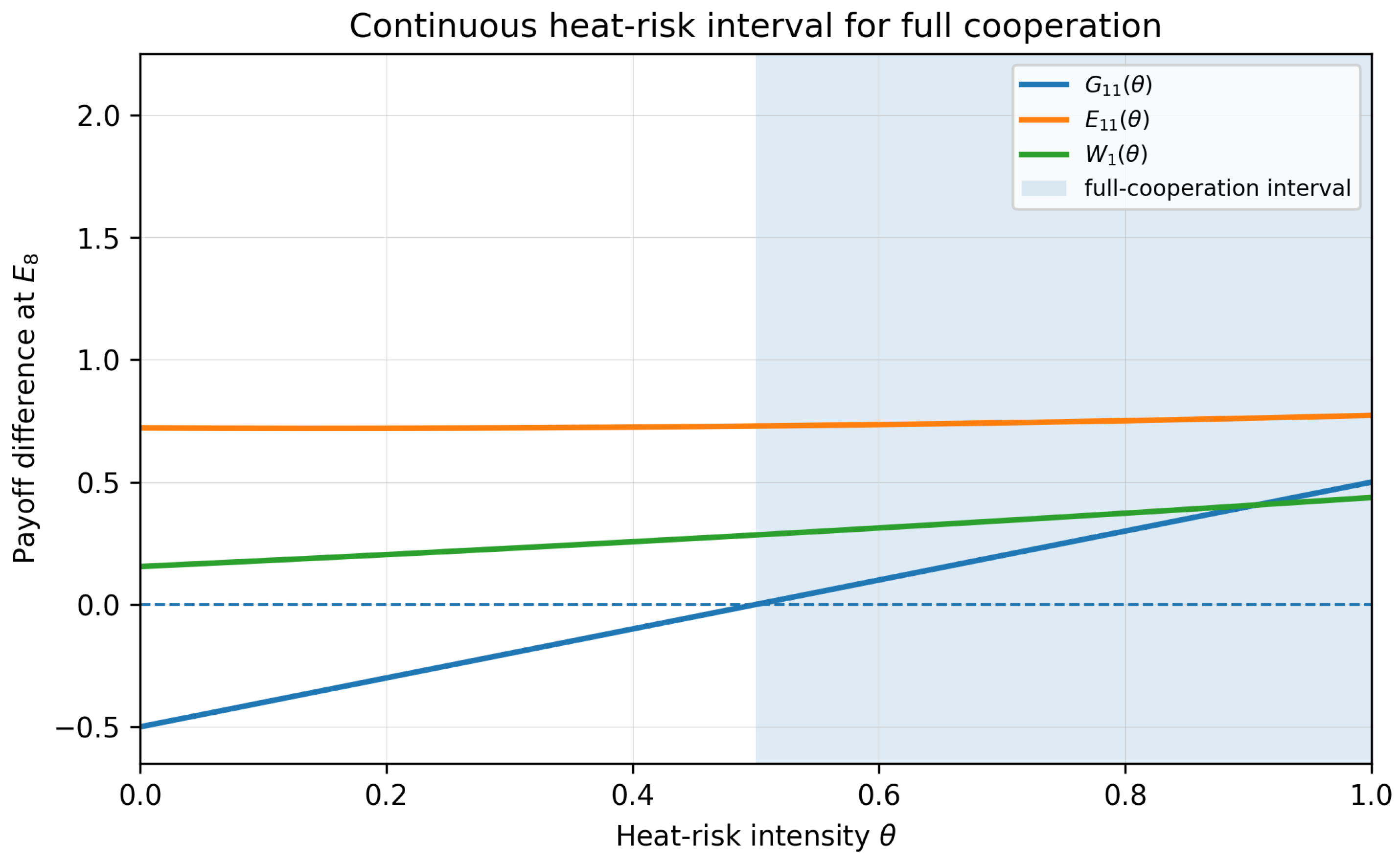
Figure 2 plots $G_{11}\left(\theta \right)$, $E_{11}\left(\theta \right)$, and $W_1\left(\theta \right)$ over the full normalized heat-risk range. The shaded area indicates the region in which all three payoff differences are positive. This figure complements the discrete mild, severe, and extreme heat simulations by showing the continuous transition from a boundary regime to the cooperative stability region.

5.9. Functional-Form Robustness of the Heat-Risk Threshold

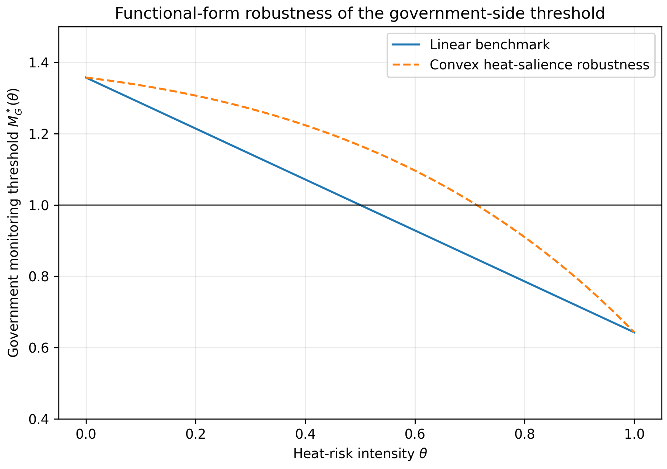
The benchmark model uses linear heat-risk functions to obtain transparent closed-form thresholds. This should be interpreted as a local linearization over the normalized range of heat-risk intensity rather than as a claim that heat-health relationships are globally linear. The stability logic extends directly to nonlinear salience functions. If the institutional benefit of strict regulation is written as $B_G\left(\theta \right)=B_{G0}+{\beta }_G{h}_B\left(\theta \right)$ and the heat-induced regulatory burden as $C_G(M,\theta )=C_{G0}-\mu M+{\chi }_G{h}_C\left(\theta \right)$, the government-side monitoring threshold becomes

$$M_G^{*}\left(\theta \right)={\displaystyle \frac{C_{G0}+S_b-B_{G0}+{\chi }_G{h}_C\left(\theta \right)-{\beta }_G{h}_B\left(\theta \right)}{\mu }}.$$

Thus, the qualitative mechanism does not require linearity: heat-risk intensity affects cooperation by shifting the relative position of institutional benefits and governance costs. Figure 3 compares the benchmark linear threshold with a convex heat-salience specification. The crossing point changes, but the central implication remains: when the required monitoring threshold lies above the feasible upper bound, the combined policy package cannot locally stabilize full cooperation.

5.10. Connection Between Stability Loss and Boundary Cycles

The stability-region result and the boundary-equilibrium result are closely connected. When $G_{11}<0$ but $W_1>0$, the cooperative equilibrium loses stability through the government-regulation direction, while the reporting face remains locally attracting. In this case, trajectories can approach the reporting face $z=1$ and move around the boundary mixed equilibrium $E_{z=1}^{*}$.

For example, under the combined policy package with $\theta =0.20$, the reporting-face mixed equilibrium is:

$$E_{z=1}^{*}=(0.621,0.842,1).$$

The system therefore does not converge monotonically to $E_8$. Instead, under the continuous-time replicator dynamics, it exhibits neutral boundary cycles around $E_{z=1}^{*}$. This explains why finite-horizon terminal values in mild heat-risk environments should not be interpreted as asymptotically stable partial-cooperation outcomes.

Remark 3. 

Proposition 3 provides local stability conditions for $E_8$. It does not establish global convergence from all initial conditions. The numerical simulations below illustrate trajectories from selected initial states, while the boundary mixed-equilibrium analysis shows that non-hyperbolic boundary dynamics may arise outside the local stability region.

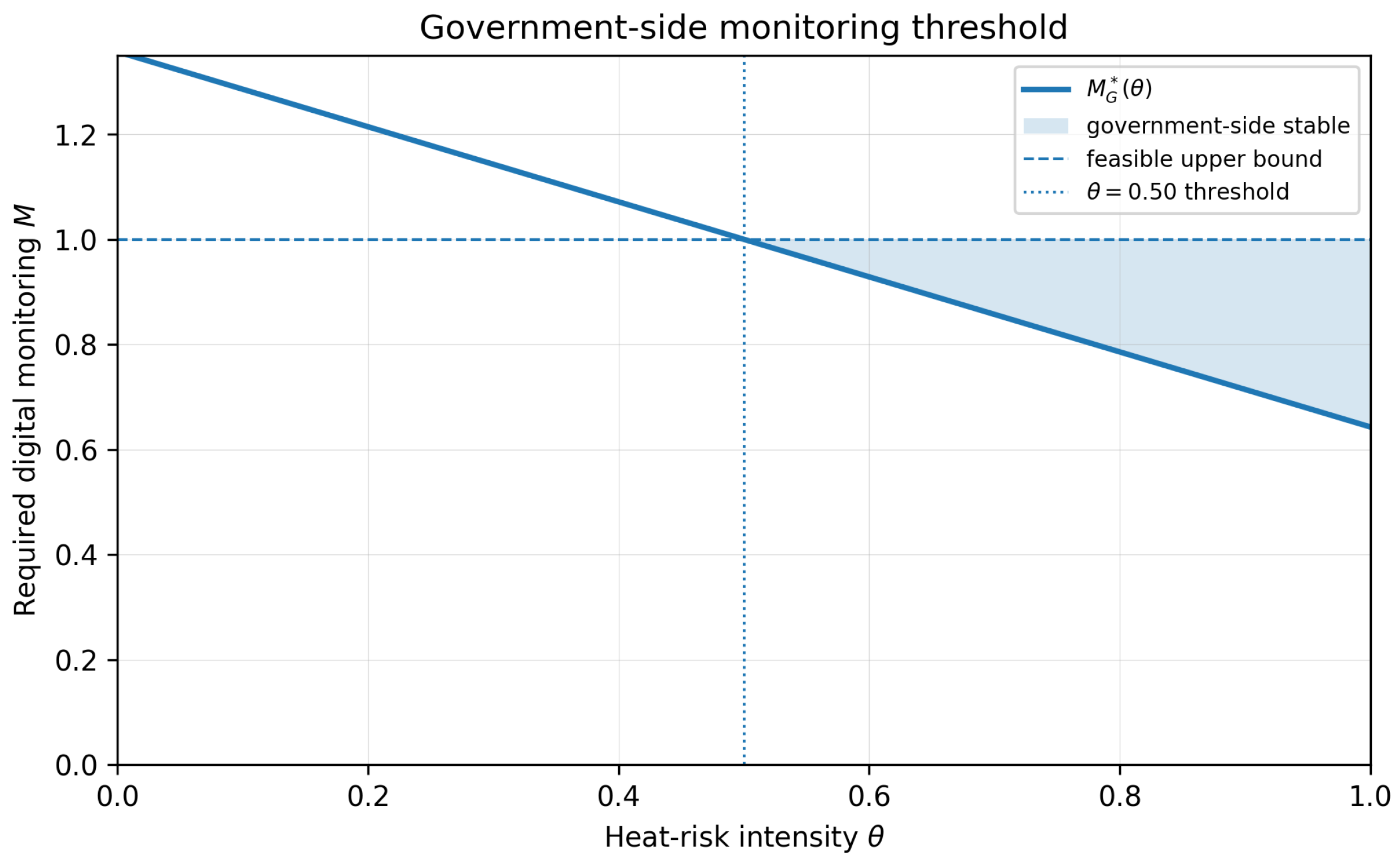
Figure 4 illustrates the government-side slice of the cooperative stability region under the combined policy package. The shaded region shows the parameter combinations in which the government-side local stability condition is satisfied, holding the remaining combined-policy parameters at their benchmark values.

6. Numerical Results

6.1. Simulation Design and Numerical Scheme

The numerical simulations illustrate the qualitative dynamic properties of the model. The theoretical model is the continuous-time replicator system in Section 5. Accordingly, the main simulations approximate the continuous-time system using a fourth-order Runge–Kutta (RK4) method. The step size is $h=0.05$, and the reported finite-horizon simulations use 3000 integration steps, corresponding to a continuous-time horizon of 150.

For comparison with discrete learning interpretations, the model can also be simulated using the forward Euler update:

$$x_{t+1}=x_t+\rho x_t(1-x_t){\Delta }_G,$$

$$y_{t+1}=y_t+\rho y_t(1-y_t){\Delta }_E,$$

$$z_{t+1}=z_t+\rho z_t(1-z_t){\Delta }_W.$$

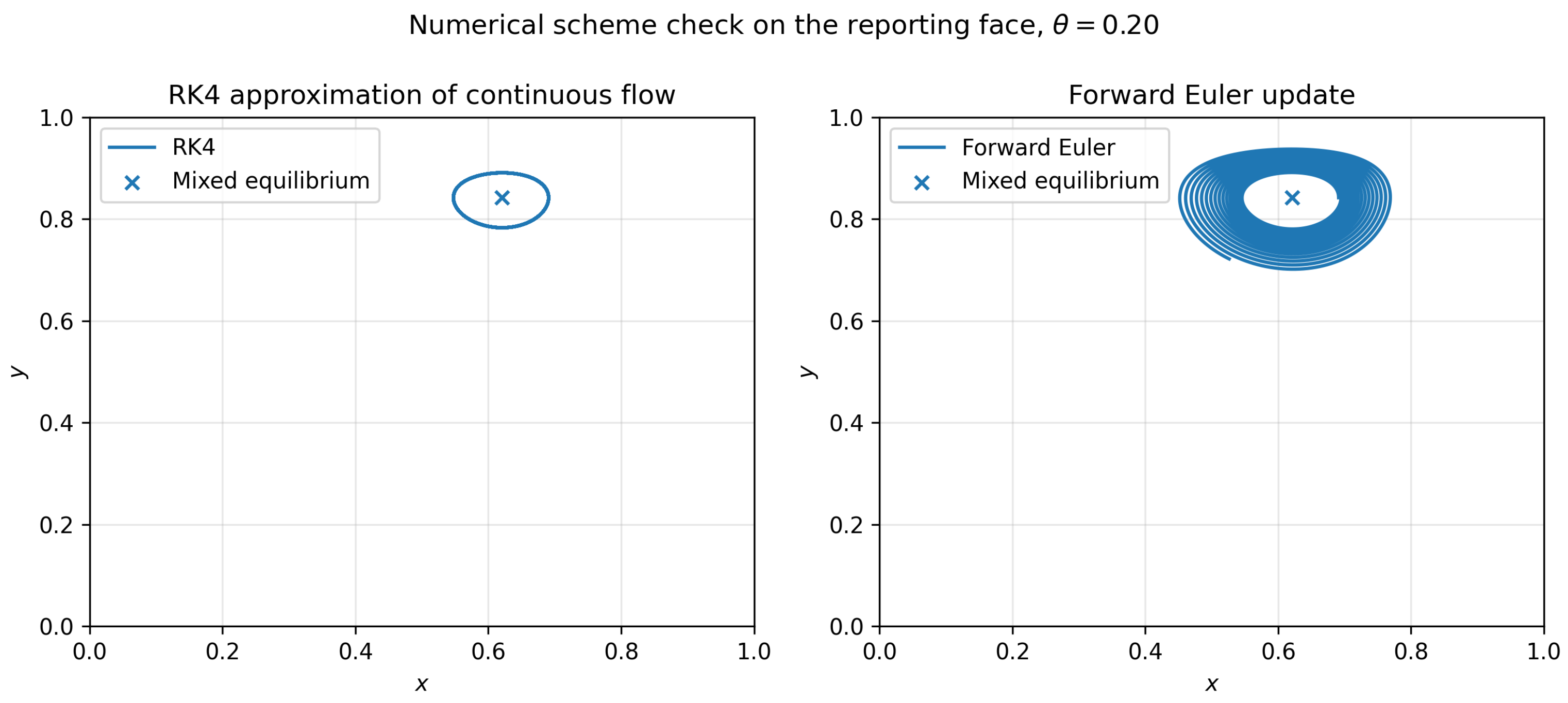
For hyperbolic pure-strategy equilibria, both schemes produce the same qualitative classification when the step size is small. However, near non-hyperbolic boundary mixed equilibria, numerical schemes may behave differently. This distinction is important because forward Euler can artificially amplify center-type motion on the reporting face. Therefore, non-hyperbolic boundary cases are interpreted qualitatively rather than through scheme-dependent terminal values.

Unless otherwise stated, the initial state is:

$$(x_0,y_0,z_0)=(0.35,0.25,0.25),$$

and the benchmark heat-risk intensity is:

$$\theta =0.60.$$

The heat-risk functions are specified as:

$$p_0\left(\theta \right)=p_{00}+{\gamma }_p\theta .$$

(22)

$$B_G\left(\theta \right)=B_{G0}+{\beta }_G\theta ,A\left(\theta \right)=A_0+{\beta }_A\theta ,$$

$$L_E\left(\theta \right)=L_{E0}+{\beta }_E\theta ,H\left(\theta \right)=H_0+{\beta }_H\theta ,$$

$$C_G(M,\theta )=C_{G0}-\mu M+{\chi }_G\theta ,C_I(M,\theta )=C_{I0}-\eta M+{\chi }_I\theta .$$

Table 7. Baseline parameter values for numerical simulations.

Parameter	Value	Meaning
$p_{00}$	0.15	Baseline heat-risk probability intercept
${\gamma }_p$	0.30	Effect of heat-risk intensity on accident probability
a	0.50	Risk reduction from employer investment
b	0.40	Risk reduction from worker reporting
$B_{G0}$	1.30	Institutional benefit intercept
${\beta }_G$	1.30	Effect of heat-risk intensity on institutional benefit
$A_0$	0.30	Governance-failure loss intercept
${\beta }_A$	0.80	Effect of heat-risk intensity on governance-failure loss
$L_{E0}$	2.70	Employer accident-loss intercept
${\beta }_E$	0.80	Effect of heat-risk intensity on employer accident loss
$H_0$	3.50	Worker health-loss intercept
${\beta }_H$	0.80	Effect of heat-risk intensity on worker health loss
$C_{G0}$	2.80	Baseline regulatory cost
$C_{I0}$	3.00	Baseline investment cost
$\mu$	1.40	Monitoring cost-reduction effect for regulation
$\eta$	1.40	Monitoring cost-reduction effect for investment
${\chi }_G$	0.30	Heat-induced increase in regulatory cost
${\chi }_I$	0.30	Heat-induced increase in investment cost
$R_E$	0.30	Employer reputation benefit
K	0.30	Safety-culture benefit to workers
$C_R$	1.20	Worker reporting cost
$q_0$	0.10	Baseline detection probability
$\alpha$	0.25	Detection effect of digital monitoring
$\lambda$	0.25	Detection effect of worker reporting

lists the normalized benchmark parameter values used in the numerical simulations.

The parameter values in Table 7 are normalized benchmark values for mechanism illustration rather than empirical estimates. They are chosen to satisfy the probability restrictions, monotonicity assumptions, and threshold structure of the model. In particular, the baseline accident probability,

$$p_0\left(\theta \right)=0.15+0.30\theta ,$$

remains in $(0,1)$ for all $\theta \in [0,1]$, and the detection probability,

$$q(M,z)=0.10+0.25M+0.25z,$$

remains below one over the feasible range of M and z. The benchmark also sets $\alpha =\lambda =0.25$, giving digital monitoring and worker reporting comparable informational effects on detection probability. The condition ${\beta }_G>{\chi }_G$ implies that heat-risk intensity raises the institutional benefit of strict regulation more strongly than it raises the regulatory cost, yielding the government-side monitoring threshold

$$M_G^{*}\left(\theta \right)={\displaystyle \frac{1.90-\theta }{1.40}}.$$

This benchmark calibration places the severe-heat case close to the cooperative stability boundary. At $\theta =0.60$,

$$M_G^{*}\left(0.60\right)=0.9286,$$

so the combined-policy value $M=1.00$ stabilizes the cooperative equilibrium, whereas reduced monitoring $M=0.80$ does not. At $\theta =0.20$,

$$M_G^{*}\left(0.20\right)=1.2143>1,$$

so the mild-heat case cannot locally stabilize full cooperation within the feasible monitoring range. The values of a and b assign a larger direct risk-reduction role to employer investment than to worker reporting, while still allowing reporting to reduce severe heat-related outcomes through early detection and response. The benchmark values are therefore selected to make the main threshold mechanisms transparent, and the sensitivity analysis below examines whether the qualitative conclusions depend on these specific numerical choices.

6.2. Policy Scenarios

The policy scenarios are defined in

Table 8. Policy scenario parameters.

Scenario	F	${\mathit{S}}_{\mathit{b}}$	M	${\mathit{P}}_{\mathit{W}}$
Baseline	0.10	0.00	0.00	0.00
Penalty only	2.50	0.00	0.00	0.00
Subsidy only	0.10	1.20	0.00	0.00
Digital monitoring only	0.10	0.00	1.00	0.00
Penalty + digital monitoring	2.50	0.00	1.00	0.00
Worker protection only	0.10	0.00	0.00	0.95
Combined policy	2.50	0.40	1.00	0.95

. The table separates true digital monitoring only from penalty plus digital monitoring. This distinction avoids attributing enforcement effects to monitoring alone.

6.3. Policy Scenario Results

Table 9. Finite-horizon simulation results under policy scenarios, $\theta =0.60$.

Scenario	Final x	Final y	Final z	Finite-Horizon Outcome
Baseline	0.000	0.000	0.000	Non-cooperative outcome
Penalty only	1.000	0.000	0.000	Regulation without employer or worker cooperation
Subsidy only	0.000	0.000	0.000	Subsidy fails without enforcement and reporting
Digital monitoring only	1.000	0.000	0.000	Monitoring-induced regulation only
Penalty + digital monitoring	1.000	0.000	0.000	Regulation without employer investment
Worker protection only	0.000	0.000	1.000	Reporting without system-wide cooperation
Combined policy	1.000	1.000	1.000	Cooperative region

reports the finite-horizon simulation results under the seven policy scenarios.

The results show that isolated policy instruments generate incomplete governance outcomes. In the baseline scenario, all three actors move toward non-cooperation. Penalties induce strict government regulation, but they do not lead to proactive employer investment or worker reporting. Subsidies alone also fail because financial support is not accompanied by effective enforcement, monitoring, or reporting incentives.

Digital monitoring only induces strict government regulation but does not induce employer investment or worker reporting. Penalty plus digital monitoring also fails to induce employer investment at the benchmark penalty level. Under the relevant boundary condition $x=1$, $z=0$, $M=1$, $S_b=0$, and $\theta =0.60$, the local employer-investment threshold is:

$$F^{*}\approx 2.73.$$

Since $F=2.50<F^{*}$, the employer payoff difference remains negative near the non-investment boundary.

This threshold should not be interpreted as a universal investment threshold. It applies to the local condition $S_b=0$ and $z=0$. Under the combined policy package, subsidies and worker reporting jointly relax the employer condition. With $S_b=0.40$ and $z=0$, the employer boundary payoff difference becomes $E_{10}=0.320>0$. With $S_b=0.40$ and $z=1$, worker reporting raises the detection probability from $q_0+\alpha M$ to $q_0+\alpha M+\lambda$, and the payoff difference becomes $E_{11}=0.735>0$. This demonstrates the complementarity of subsidies, monitoring, and reporting.

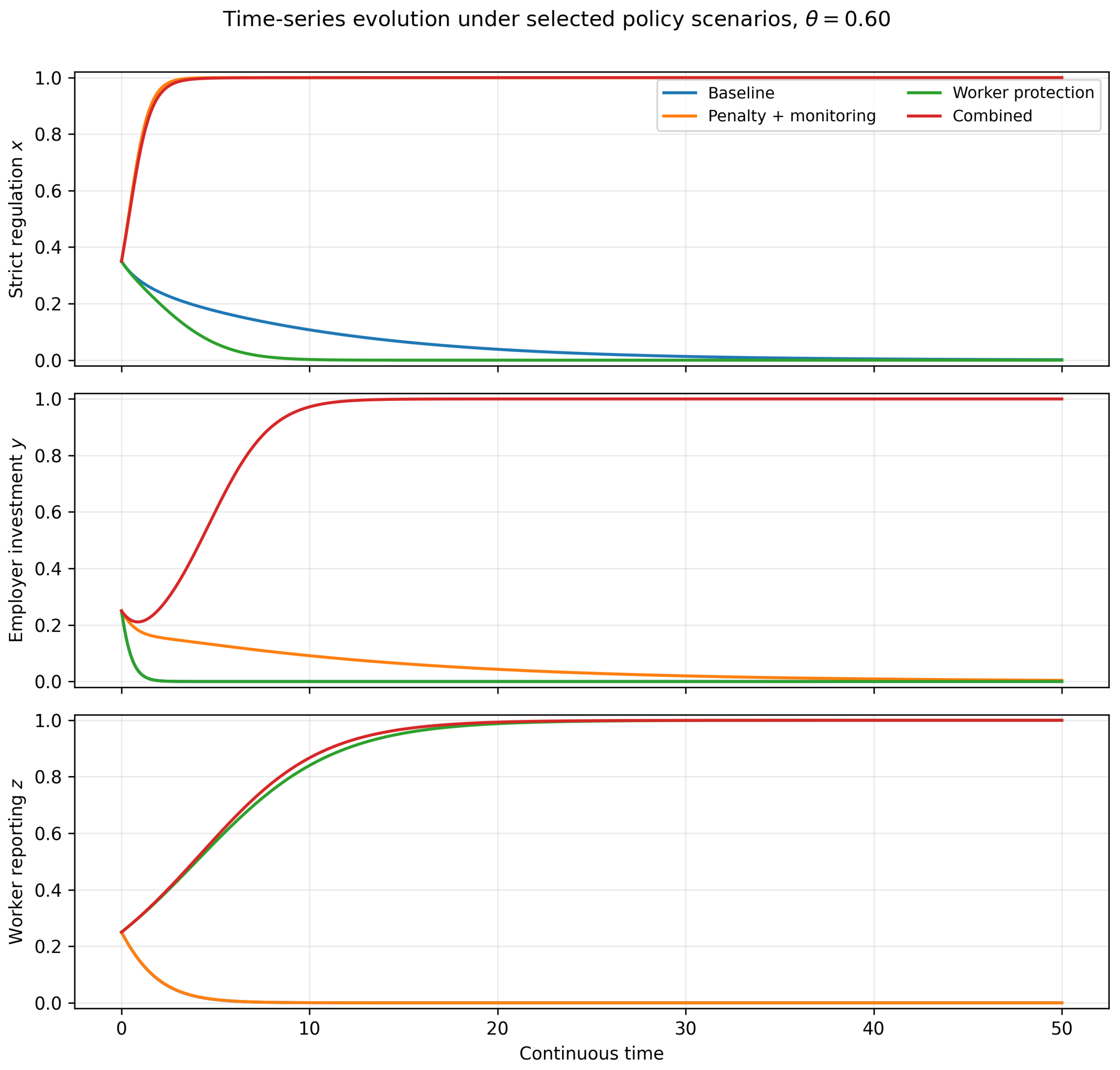
6.4. Time-Series Evolution Under Selected Policy Scenarios

Figure 5 reports the standard evolutionary time paths for selected policy scenarios at $\theta =0.60$. This figure complements the finite-horizon classification in Table 9 by showing the speed and direction of adjustment for the three state variables. The combined policy package moves all three trajectories toward the cooperative region. By contrast, penalty plus monitoring raises strict regulation but does not induce employer investment or worker reporting, while worker protection alone increases reporting without generating system-wide cooperation.

6.5. Temperature-Shock Simulation

To examine whether heat-risk intensity alters the evolutionary outcome, this subsection compares:

$$\theta =0.20,\theta =0.60,\theta =1.00.$$

These values represent mild heat exposure, severe heat exposure, and extreme heatwave conditions.

Table 10. Temperature-shock simulation under baseline policy.

Heat-Risk Intensity	Final x	Final y	Final z	Outcome
$\theta =0.20$	0.000	0.000	0.000	Non-cooperation
$\theta =0.60$	0.000	0.000	0.000	Non-cooperation
$\theta =1.00$	1.000	0.000	0.000	Regulatory response only

reports the temperature-shock simulations under the baseline policy setting, while

Table 11. Temperature-shock simulation under the combined policy package.

Heat-Risk Intensity	Local Status of ${\mathit{E}}_8$	Diagnostic Object	Outcome Interpretation
$\theta =0.20$	Unstable	$E_{z=1}^{*}=(0.621,0.842,1)$	Neutral boundary cycle
$\theta =0.60$	Stable	$E_8=(1,1,1)$	Cooperative region
$\theta =1.00$	Stable	$E_8=(1,1,1)$	Cooperative region

reports the corresponding simulations under the combined policy package.

Under weak policy settings, mild and severe heat-risk conditions lead to non-cooperation. Extreme heat induces only a regulatory response. Thus, heat shocks can activate government regulation, but they do not automatically induce employer investment or worker reporting.

Under the combined policy package, severe and extreme heat-risk conditions stabilize the cooperative equilibrium. Under mild heat-risk intensity, however, $M_G^{*}\left(0.20\right)=1.2143>1$, so $E_8$ cannot be locally stabilized under any feasible value of $M\le 1$. The relevant dynamic object is instead the boundary mixed equilibrium on the reporting face.

6.6. Numerical-Scheme Check for Non-Hyperbolic Boundary Dynamics

Because the theoretical model is continuous-time but some finite-horizon simulations can be implemented through discrete updates, it is important to check whether boundary dynamics are sensitive to the numerical scheme. Figure 6 compares the fourth-order Runge–Kutta approximation of the continuous-time flow with the forward Euler update on the reporting face under the combined policy package with $\theta =0.20$.

The RK4 approximation remains close to center-type cyclic motion around the boundary mixed equilibrium, whereas the forward Euler update can amplify the cycle and push trajectories toward the boundary. Therefore, quantitative statistics such as the share of time spent in the cooperative region should not be over-interpreted for non-hyperbolic boundary cases. The qualitative conclusion is that mild heat-risk intensity does not generate asymptotic convergence to the pure cooperative equilibrium, even under the combined policy package.

6.7. Perturbation Check for Boundary-Cycle Geometry

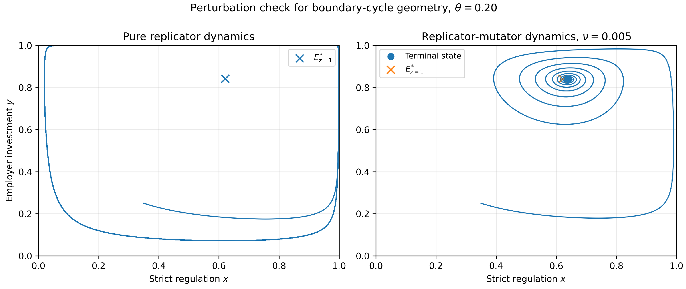
Because the reporting-face mixed equilibrium is non-hyperbolic, its cycle geometry is structurally sensitive. To check whether the neutral cycle is a robust attractor or a feature of the pure replicator dynamic, I also simulate a weak symmetric replicator–mutator perturbation,

$${\dot{s}}_i=s_i(1-s_i){\Delta }_i+\nu (1-2s_i),s_i\in \{x,y,z\},$$

where $\nu >0$ represents low-rate exploration, mutation, or behavioral experimentation. This perturbation is not introduced as an alternative main model; it is a diagnostic for the structural robustness of the boundary-cycle geometry. Figure 7 shows that the pure replicator system displays center-type motion on the reporting face, whereas a weak mutation term with $\nu =0.005$ removes the exact neutral center and produces convergence toward a nearby perturbed regime. In the benchmark perturbation, the trajectory converges to approximately

$$(x,y,z)=(0.639,0.838,0.973),$$

which is characterized by high reporting and intermediate regulation and investment rather than convergence to the fully cooperative equilibrium $E_8=(1,1,1)$. Thus, the robust conclusion is not the exact closed-orbit geometry itself, but the failure of the system to converge to full cooperation under mild heat-risk intensity. In the pure replicator system this failure appears as a neutral boundary cycle around $E_{z=1}^{*}$; under weak mutation it appears as convergence to a nearby partial-cooperation regime. The exact location of the perturbed limit depends on the perturbation family and perturbation strength. Symmetric mutation, logit adjustment, and finite-population noise need not produce identical limiting states. However, they share the implication that the non-hyperbolic center is structurally fragile.

This result is consistent with the classical observation that non-hyperbolic centers in replicator dynamics can be sensitive to perturbations of the adjustment rule [24].

6.8. Phase-Space Trajectories

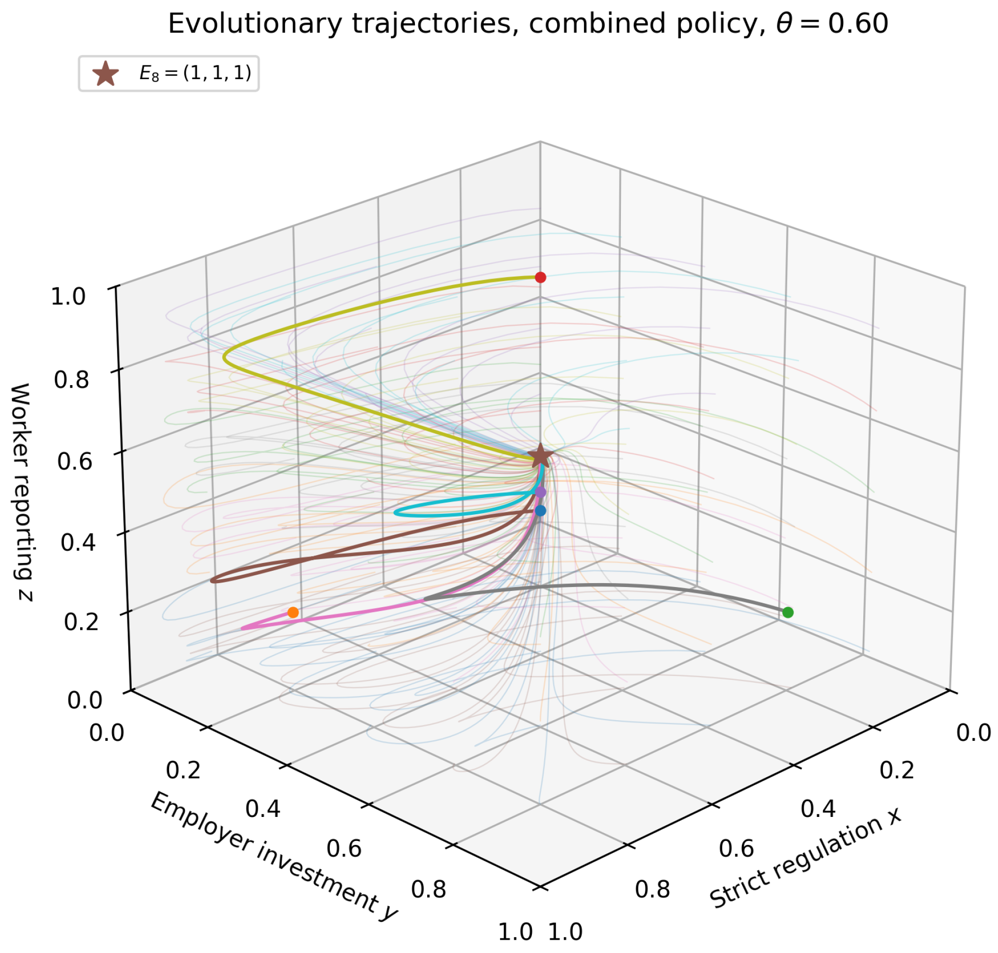
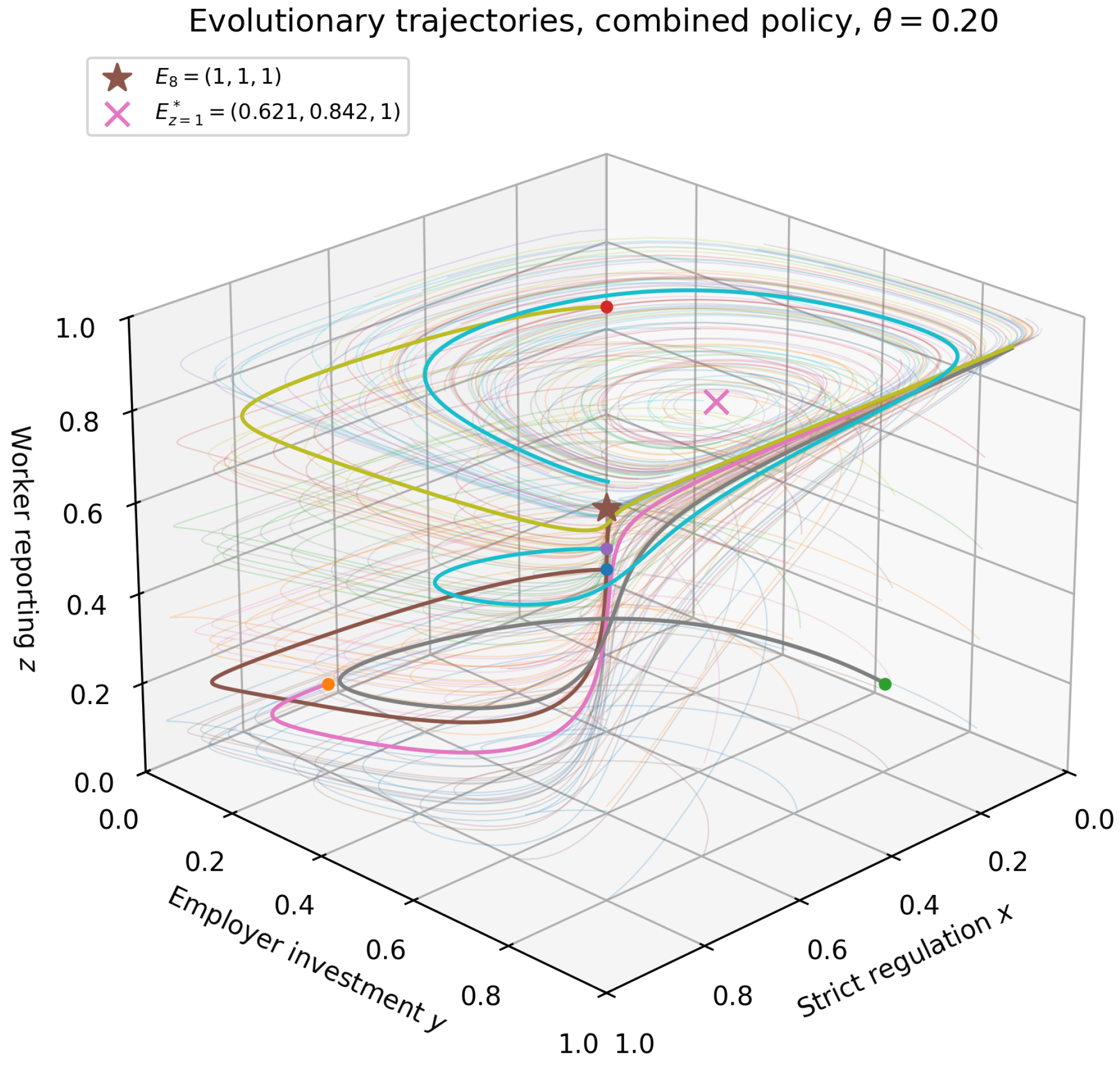
To visualize the global movement of the evolutionary system under different heat-risk conditions, this subsection reports phase-space trajectories from multiple interior initial states. Figure 8 shows the severe-heat case under the combined policy package with $\theta =0.60$. Consistent with the local-stability analysis, trajectories from a grid of interior initial conditions move toward the cooperative equilibrium $E_8=(1,1,1)$ within the simulated horizon.

Figure 9 reports the corresponding mild-heat case with $\theta =0.20$. In this case, the cooperative equilibrium is not locally stable because the government-side monitoring threshold exceeds the feasible upper bound. The trajectories therefore move toward the reporting face and circulate around the boundary mixed equilibrium $E_{z=1}^{*}$, indicating neutral boundary-cycle dynamics rather than convergence to full cooperation.

6.9. Finite-Horizon Regime Diagnostics

Local stability analysis identifies whether an equilibrium is stable in its neighborhood. It does not, however, establish how the system behaves from a broader set of initial conditions. To complement the local analysis, this subsection reports finite-horizon regime diagnostics based on randomized initial states. Initial conditions are sampled uniformly from ${[0.02,0.98]}^3$, and the continuous-time replicator system is integrated using the fourth-order Runge–Kutta method. A terminal state is classified as cooperative if $x>0.99$, $y>0.99$, and $z>0.99$. The resulting shares should be interpreted as finite-horizon attainability diagnostics rather than estimates of global convergence probabilities.

Table 12. Finite-horizon regime diagnostics from randomized initial states.

Scenario	Cooperative	Non-Cooperative	Regulation Only	Investment Without Reporting	Reporting-Face/Cycle	Other Incomplete
Baseline, $\theta =0.60$	0.000	1.000	0.000	0.000	0.000	0.000
Combined, $\theta =0.20$	0.038	0.000	0.000	0.000	0.954	0.008
Combined, $\theta =0.60$	1.000	0.000	0.000	0.000	0.000	0.000
Reduced monitoring, $M=0.80,\theta =0.60$	0.243	0.000	0.000	0.000	0.754	0.003
Low reporting protection, $P_W=0.40,\theta =0.60$	0.000	0.000	0.000	1.000	0.000	0.000

Notes: Shares are finite-horizon diagnostics based on $N=1000$ initial conditions sampled uniformly from ${[0.02,0.98]}^3$. The continuous-time replicator system is integrated with the fourth-order Runge–Kutta method using step size $h=0.05$ for 3000 steps, corresponding to a continuous-time horizon $T=150$. A terminal state is classified as cooperative if $x>0.99$, $y>0.99$, and $z>0.99$. Shares may not sum exactly to one due to rounding. These estimates compare finite-horizon attainability across policy regimes and should not be interpreted as exact global convergence probabilities.

reports the finite-horizon regime shares obtained from randomized interior initial states.

Table 12 supports the local stability analysis while also clarifying the limits of finite-horizon simulation. Under the baseline policy at $\theta =0.60$, all sampled trajectories move toward the non-cooperative regime. Under the combined policy package at $\theta =0.60$, the cooperative regime is reached from all sampled interior initial states at the simulation horizon, which is consistent with the local stability of $E_8=(1,1,1)$. By contrast, under the combined policy package at $\theta =0.20$, most trajectories enter the reporting-face/cycle regime rather than converging to full cooperation. This result is consistent with the threshold condition $M_G^{*}\left(0.20\right)>1$, which implies that the cooperative equilibrium cannot be locally stabilized under the feasible monitoring range $M\le 1$.

The low-reporting-protection case illustrates why the classification must distinguish incomplete governance regimes. When $P_W=0.40$, the system converges to $E_7=(1,1,0)$, namely strict regulation and employer investment without worker reporting. This regime is neither full cooperation nor regulation only; it is therefore reported as “investment without reporting.” The reduced-monitoring case also requires careful interpretation. Since $M=0.80<M_G^{*}\left(0.60\right)=0.9286$, the cooperative equilibrium is locally unstable in the government-regulation direction. The finite-horizon cooperative share reported in Table 12 reflects long transient behavior near the cooperative corner when the instability margin is modest; it should not be interpreted as asymptotic convergence to $E_8$.

Overall, the finite-horizon diagnostics reinforce the main theoretical result. In these simulations, full cooperation is attained broadly only when the combined policy package moves the system into the cooperative stability region. When heat-risk intensity is mild or monitoring falls below the government-side threshold, trajectories are more likely to remain in partial-cooperation regimes, especially the reporting-face/cycle regime. These results should be read together with the local stability thresholds and the boundary-cycle analysis rather than as a separate proof of global convergence.

7. Sensitivity Analysis

The sensitivity analysis examines robustness to initial conditions, parameter perturbations, and policy complementarity. Unless otherwise stated, the combined policy package is used, heat-risk intensity is $\theta =0.60$, and the simulation uses RK4 with 3000 integration steps. A system is classified as being in the cooperative region at the simulation horizon if:

$$x>0.99,y>0.99,z>0.99.$$

This classification is a finite-horizon diagnostic criterion, not a proof of global convergence.

7.1. Robustness to Initial Conditions

Six alternative initial conditions are considered.

Table 13. Sensitivity analysis: alternative initial conditions under the combined policy package.

Initial Condition (${\mathit{x}}_0,{\mathit{y}}_0,{\mathit{z}}_0$)	Final x	Final y	Final z	First Hitting Time
$(0.2,0.2,0.2)$	1.000	1.000	1.000	396
$(0.5,0.5,0.5)$	1.000	1.000	1.000	299
$(0.8,0.2,0.2)$	1.000	1.000	1.000	392
$(0.2,0.8,0.2)$	1.000	1.000	1.000	389
$(0.2,0.2,0.8)$	1.000	1.000	1.000	218
$(0.8,0.8,0.8)$	1.000	1.000	1.000	457

reports terminal values and the first hitting time of the cooperative region.

The combined policy package reaches the cooperative region from all six initial conditions at the benchmark heat-risk intensity. This supports the relevance of the local stability result around $E_8$, although it does not prove global convergence for all possible initial states.

7.2. Robustness to Parameter Perturbations

Table 14. Sensitivity analysis: $\pm 20\%$ parameter perturbations under the combined policy package.

Parameter	Perturbation	Actual Value	Final x	Final y	Final z	Finite-Horizon Outcome
F	$-20\%$	2.000	1.000	1.000	1.000	Cooperative region
F	$+20\%$	3.000	1.000	1.000	1.000	Cooperative region
$S_b$	$-20\%$	0.320	1.000	1.000	1.000	Cooperative region
$S_b$	$+20\%$	0.480	1.000	1.000	1.000	Cooperative region
M	$-20\%$	0.800	1.000	0.383	1.000	Outside stability region; boundary-cycle case
M	$+20\%$	1.000	1.000	1.000	1.000	Cooperative region
$P_W$	$-20\%$	0.760	1.000	1.000	1.000	Cooperative region
$P_W$	$+20\%$	1.140	1.000	1.000	1.000	Cooperative region
$C_R$	$-20\%$	0.960	1.000	1.000	1.000	Cooperative region
$C_R$	$+20\%$	1.440	1.000	1.000	1.000	Cooperative region
$C_{G0}$	$-20\%$	2.240	1.000	1.000	1.000	Cooperative region
$C_{G0}$	$+20\%$	3.360	0.984	0.445	1.000	Outside stability region; boundary-cycle case
$C_{I0}$	$-20\%$	2.400	1.000	1.000	1.000	Cooperative region
$C_{I0}$	$+20\%$	3.600	1.000	1.000	1.000	Cooperative region
$H_0$	$-20\%$	2.800	1.000	1.000	1.000	Cooperative region
$H_0$	$+20\%$	4.200	1.000	1.000	1.000	Cooperative region
$\theta$	$-20\%$	0.480	0.995	1.000	1.000	Locally unstable $E_8$; slow finite-horizon drift
$\theta$	$+20\%$	0.720	1.000	1.000	1.000	Cooperative region

Notes: For M, the +20% perturbation is capped at the feasible upper bound M = 1. The M − 20%, C_G0 + 20%, and θ − 20% cases lie outside the local stability region of E₈ through the government-regulation condition. In particular, when θ = 0.48, $M_G^{*}(0.48)=\frac{1.90-0.48}{1.40}=1.014>1$, so G₁₁ < 0 under the feasible value M = 1. The terminal value (0.995, 1.000, 1.000) should therefore be interpreted as a near-cooperative finite-horizon snapshot close to the stability boundary rather than as asymptotic convergence to the cooperative equilibrium. This interpretation is consistent with the finite-horizon diagnostic logic used in Table 12 and Table 15.

perturbs key parameters by $\pm 20\%$ around the combined-policy benchmark.

Most moderate perturbations preserve the cooperative-region outcome at the finite horizon. However, reducing M or increasing $C_{G0}$ moves the system outside or near the boundary of the government stability region. These cases should be interpreted through the stability condition $G_{11}>0$ rather than as direct employer-side failures. For M, the $+20\%$ perturbation is capped at the feasible upper bound $M=1$.

7.3. Policy Complementarity Between Digital Monitoring and Worker Protection

The final sensitivity check examines the interaction between digital monitoring M and worker reporting protection $P_W$. This diagnostic is important because the model implies that the two instruments affect different parts of the dynamic system. Digital monitoring M improves technological visibility by increasing detection probability and reducing governance and investment costs. Worker reporting protection $P_W$, by contrast, directly affects the worker reporting payoff difference ${\Delta }_W$.

To avoid conflating these two mechanisms,

Table 15. Policy-complementarity diagnostics: terminal strategy shares $(x,y,z)$.

M	${\mathit{P}}_{\mathit{W}}$
	0.00	0.40	0.80	0.95	1.20
0.00 †	$(1.000,0.000,0.000)$	$(1.000,0.000,0.000)$	$(0.055,0.000,1.000)$	$(0.022,0.000,1.000)$	$(0.016,0.000,1.000)$
0.25 †	$(1.000,0.000,0.000)$	$(1.000,0.000,0.000)$	$(1.000,0.000,1.000)$	$(1.000,0.000,1.000)$	$(1.000,0.000,1.000)$
0.50 †	$(1.000,0.000,0.000)$	$(1.000,0.000,0.000)$	$(1.000,0.000,1.000)$	$(1.000,0.000,1.000)$	$(1.000,0.000,1.000)$
0.75 †	$(1.000,0.000,0.000)$	$(1.000,0.000,0.000)$	$(1.000,1.000,1.000)$	$(1.000,0.107,1.000)$	$(1.000,0.996,1.000)$
1.00	$(1.000,1.000,0.000)$	$(1.000,1.000,0.000)$	$(1.000,1.000,1.000)$	$(1.000,1.000,1.000)$	$(1.000,1.000,1.000)$

Notes: Rows marked with ^† have $M<M_G^{*}(0.60)=0.9286$ and therefore lie outside the local stability region of E₈. The reported values in those rows are finite-horizon snapshots and may reflect the phase of non-convergent boundary or near-boundary dynamics rather than asymptotic outcomes. In particular, the non-monotonic values in the M = 0.75 row should not be interpreted as a comparative-static effect of worker protection.

reports terminal strategy shares at the finite horizon for a grid of M and $P_W$. The rows vary digital monitoring within the feasible interval $M\in [0,1]$, while the columns vary worker reporting protection. Other parameters are held at the combined-policy benchmark:

$$F=2.50,S_b=0.40,\theta =0.60.$$

Cells with $M<M_G^{*}\left(0.60\right)=0.9286$ lie outside the local stability region of $E_8$, so their terminal values should be interpreted as finite-horizon diagnostics rather than asymptotic outcomes.

The grid clarifies the distinct roles of M and $P_W$. Since the worker payoff difference ${\Delta }_W$ does not contain M, digital monitoring alone cannot directly induce worker reporting. Consistent with this structure, the transition of z from zero to one is primarily governed by $P_W$. When $P_W$ is low, workers do not report even if digital monitoring is high. When $P_W$ is sufficiently high, reporting becomes attractive and z moves toward one.

Digital monitoring affects a different part of the system. As shown in the stability-region analysis, the government-side condition around the cooperative equilibrium is governed by $M>M_G^{*}\left(\theta \right)$. At $\theta =0.60$, the benchmark threshold is $M_G^{*}\left(0.60\right)=0.9286$. Therefore, the row $M=1.00$ lies inside the local stability region of $E_8$, while lower values of M may generate finite-horizon outcomes that do not represent asymptotic convergence to the cooperative equilibrium. The apparent non-monotonicity in the $M=0.75$ row should therefore not be interpreted as a comparative-static effect of worker protection; it reflects finite-horizon phase snapshots outside the cooperative stability region.

The table therefore supports a sharper complementarity interpretation. Worker reporting protection creates institutional trust and directly stabilizes z. Digital monitoring improves detectability and stabilizes government regulation, which then indirectly supports employer investment. Full cooperation requires both a sufficiently high level of worker protection and a sufficiently high level of digital monitoring. When either instrument is weak, the system may remain in an incomplete governance state or exhibit neutral boundary cycles rather than converge to $E_8$.

7.4. Semi-Empirical Accident-Risk Calibration Check

The benchmark simulations above use normalized parameter values to make the threshold mechanisms transparent. As an additional robustness check, this subsection links the accident-risk component of the model to empirical evidence from Fu and Sasaki [14]. Their prefecture-month estimates for Japan show that one additional day with a maximum daily temperature exceeding $35°\mathrm{C}$ increases monthly work-related injuries by 3.145 cases in the preferred specification, relative to the 20–$25°\mathrm{C}$ reference interval. The sample mean of monthly prefecture-level injuries is 214.88. This implies an approximate per-day relative injury-risk increase of

$${\widehat{r}}_{35}={\displaystyle \frac{3.145}{214.88}}=0.0146.$$

This estimate is used to construct a semi-empirical accident-risk calibration for the slope parameter ${\gamma }_p$ in

$$p_0\left(\theta \right)=p_{00}+{\gamma }_p\theta .$$

The purpose is not to estimate a structural accident probability, but to check whether the model’s qualitative conclusions are robust when the heat-risk slope is disciplined by observed heat–injury estimates. Let a full-unit increase in the normalized heat-risk index $\theta$ correspond to an illustrative increase of $\Delta D=20$ extreme-heat days over the relevant exposure horizon. With $p_{00}=0.15$, the semi-empirical central slope is

$${\gamma }_p^C=p_{00}{\widehat{r}}_{35}\Delta D=0.15\times 0.0146\times 20=0.044.$$

To account for statistical uncertainty in the empirical estimate, lower- and upper-bound slopes are also constructed using the reported standard error of 0.957:

$${\widehat{r}}_{35}^L={\displaystyle \frac{3.145-1.96\left(0.957\right)}{214.88}}=0.0059,$$

$${\widehat{r}}_{35}^H={\displaystyle \frac{3.145+1.96\left(0.957\right)}{214.88}}=0.0234.$$

This gives

$${\gamma }_p^L=0.15\times 0.0059\times 20=0.018,$$

and

$${\gamma }_p^H=0.15\times 0.0234\times 20=0.070.$$

Table 16. Semi-empirical calibration of the accident-risk slope.

Calibration	Empirical Input	Calibrated ${\mathit{\gamma }}_{\mathit{p}}$	Implied ${\mathit{p}}_0$(1)
Lower-bound estimate	$3.145-1.96\left(0.957\right)$	0.018	0.168
Central estimate	$3.145$	0.044	0.194
Upper-bound estimate	$3.145+1.96\left(0.957\right)$	0.070	0.220
Benchmark model	Normalized mechanism value	0.300	0.450

reports the semi-empirical calibration of the accident-risk slope and compares it with the normalized benchmark value.

Table 16 shows that the empirically informed accident-risk slopes are more conservative than the normalized benchmark value used in the main simulations. This is expected because the benchmark is designed to illustrate the full threshold structure of the governance system, whereas the semi-empirical check uses reduced-form estimates of the observed heat–injury relationship. Importantly, the qualitative stability logic is unchanged. The government-side monitoring threshold,

$$M_G^{*}\left(\theta \right)={\displaystyle \frac{1.90-\theta }{1.40}},$$

does not depend on ${\gamma }_p$. Therefore, the mild-heat case still cannot locally stabilize full cooperation because $M_G^{*}\left(0.20\right)=1.2143>1$, while the severe-heat benchmark remains inside the government-side stability region because $M_G^{*}\left(0.60\right)=0.9286<1$.

The semi-empirical calibration mainly affects the employer and worker payoff differences through the accident-risk term. Under the combined policy package and $\theta =0.60$, all three semi-empirical values of ${\gamma }_p$ continue to satisfy the employer and worker stability conditions, $E_{11}>0$ and $W_1>0$. Thus, the main conclusion is robust: full cooperation is not generated by heat risk alone, but becomes locally stable when monitoring capacity, enforcement incentives, employer investment support, and protected worker reporting are jointly strong enough.

Table 17. Empirical and institutional anchors for normalized model parameters.

Parameter Group	Empirical or Institutional Anchor	Treatment in the Revised Manuscript
$p_0\left(\theta \right),{\gamma }_p$	Japan prefecture-level heat–injury estimates from Fu and Sasaki	Semi-empirical slope calibration in Table 16
$F,S_b,P_W$	Policy levers corresponding to penalties, employer support, and reporting protection under the 2025 reform	Scenario parameters varied across policy packages
$q_0,\alpha ,\lambda$	Detection logic from deterrence and monitoring theory	Normalized values with sensitivity to monitoring and reporting channels
$C_G,C_I$	Administrative and employer prevention costs	Normalized cost parameters, perturbed in Table 14
$L_E,H,C_R$	Employer losses, worker health/wage losses, and reporting costs	Reduced-form loss parameters; extended interpretation includes reputation and wage-loss components

summarizes how the normalized parameters are externally anchored. The purpose is not to claim structural estimation of all parameters, but to make transparent which parameters are linked to empirical or institutional information and which remain normalized mechanism parameters explored through sensitivity analysis.

7.5. Robustness to Government-Failure Payoff Normalization

The benchmark payoff matrix normalizes the government’s lenient-regulation payoff to zero except in the state $(L,P,C)$, where governance failure creates the loss $-A\left(\theta \right)$. This specification makes the cost of leniency state-dependent and concentrates the governance-failure loss in the case where neither employer investment nor worker reporting mitigates the risk. Because this normalization is strong, I examine an alternative specification in which lenient regulation generates an expected failure loss proportional to the heat-related accident probability:

$${\tilde{U}}_G^L=-A\left(\theta \right)p(y,z;\theta ).$$

Under this alternative specification, the government payoff difference becomes

$${\tilde{\Delta }}_G=B_G\left(\theta \right)-C_G(M,\theta )-S_{b}y+q(M,z)F(1-y)+A\left(\theta \right)p_0\left(\theta \right)(1-ay)(1-bz).$$

At the cooperative equilibrium $E_8=(1,1,1)$, the government-side stability condition is

$$B_G\left(\theta \right)-C_G(M,\theta )-S_b+A\left(\theta \right)p_0\left(\theta \right)(1-a)(1-b)>0.$$

Thus, the alternative government-side monitoring threshold is

$${\tilde{M}}_G^{*}\left(\theta \right)={\displaystyle \frac{C_{G0}+S_b-B_{G0}+({\chi }_G-{\beta }_G)\theta -A\left(\theta \right)p_0\left(\theta \right)(1-a)(1-b)}{\mu }}.$$

Table 18. Robustness of the government-side monitoring threshold under alternative leniency-loss specification.

Heat-Risk Intensity	Benchmark ${\mathit{M}}_{\mathit{G}}^{*}\mathsf{\left(}\mathit{\theta }\mathsf{\right)}$	Alternative ${\tilde{\mathit{M}}}_{\mathit{G}}^{*}\mathsf{\left(}\mathit{\theta }\mathsf{\right)}$	Interpretation
$\theta =0.20$	1.214	1.194	Still above feasible $M=1$
$\theta =0.60$	0.929	0.873	Still stabilizable under $M=1$
$\theta =1.00$	0.643	0.537	Stable region expands further

summarizes the government-side monitoring threshold under the benchmark and alternative leniency-loss specifications.

Table 18 shows that the qualitative threshold logic is unchanged. Because the alternative specification assigns a residual expected governance-failure loss even when employer investment and worker reporting reduce accident risk, it lowers the monitoring threshold relative to the benchmark specification. However, the central conclusion remains the same: the mild-heat case still cannot locally stabilize full cooperation within the feasible monitoring range, whereas the severe-heat and extreme-heat cases remain inside the government-side stability region under the combined policy package. The benchmark normalization therefore does not drive the main mild-heat result.

The alternative specification also preserves the qualitative structure of the mild-heat reporting-face dynamics. Under this specification, ${\Delta }_W$ is unchanged. On the reporting face $z=1$, ${\tilde{\Delta }}_G$ remains linear in y, while ${\Delta }_E$ remains linear in x. Therefore, the reporting-face mixed equilibrium remains a zero-trace center in the tangent $(x,y)$ dynamics, although its position changes slightly.

Under the combined policy package with $\theta =0.20$, the employer indifference condition is unchanged, so

$${\tilde{x}}_1^{*}=x_1^{*}=0.621.$$

The government indifference condition becomes

$${\tilde{y}}_1^{*}={\displaystyle \frac{B_G\left(\theta \right)-C_G(M,\theta )+FQ\left(1\right)+A\left(\theta \right)p_0\left(\theta \right)(1-b)}{S_b+FQ\left(1\right)+A\left(\theta \right)p_0\left(\theta \right)a(1-b)}},$$

which gives

$${\tilde{y}}_1^{*}=0.859.$$

Thus, the reporting-face mixed equilibrium moves from

$$E_{z=1}^{*}=(0.621,0.842,1)$$

in the benchmark specification to approximately

$${\tilde{E}}_{z=1}^{*}=(0.621,0.859,1)$$

under the failure-proportional leniency-loss specification. The mild-heat conclusion is therefore unchanged: the system is pushed toward the reporting face, but it does not converge asymptotically to the full cooperative equilibrium $E_8$.

This robustness check addresses the normalization of lenient-regulation failure losses. The next subsections further relax two additional benchmark assumptions by allowing monitoring and regulatory strictness to enter worker reporting incentives directly and by linking government payoffs to accident-risk reduction rather than regulatory action alone.

7.6. Extended Worker Reporting Payoff with Monitoring and Regulatory Effects

The benchmark model separates digital monitoring and worker reporting protection into two distinct channels. Digital monitoring M affects the visibility–enforcement channel by increasing detection probability and reducing governance and investment costs, whereas worker reporting protection $P_W$ directly affects the reporting–trust channel. This separation clarifies the baseline mechanism, but it may understate the possibility that monitoring technology and regulatory strictness also influence workers’ willingness to report symptoms.

In practice, digital monitoring can affect worker reporting incentives through several mechanisms. WBGT sensors, wearable devices, and digital heat-warning systems can provide objective evidence that reduces ambiguity about whether a heat-risk condition exists. Monitoring records may also reduce the expected burden of proving that symptoms are work-related. Similarly, stricter regulatory enforcement can increase workers’ confidence that reported symptoms will trigger an organizational response rather than being ignored or punished. To examine whether the main conclusions depend on the benchmark exclusion of these direct reporting effects, I introduce an extended worker-payoff specification.

Let ${\psi }_M\ge 0$ denote the direct reporting-incentive effect of digital monitoring, and let ${\psi }_x\ge 0$ denote the direct reporting-incentive effect of regulatory strictness. The extended payoff of worker reporting is defined as

$${\tilde{U}}_W^R=P_W+yK+{\psi }_{M}M+{\psi }_{x}x-C_R-H\left(\theta \right)p_0\left(\theta \right)(1-ay)(1-b).$$

(23)

The payoff of continuing work remains

$${\tilde{U}}_W^C=-H\left(\theta \right)p_0\left(\theta \right)(1-ay).$$

(24)

Therefore, the extended worker payoff difference is

$${\tilde{\Delta }}_W=P_W+yK-C_R+H\left(\theta \right)p_0\left(\theta \right)b(1-ay)+{\psi }_{M}M+{\psi }_{x}x.$$

(25)

Equation (25) nests the benchmark model as the special case ${\psi }_M={\psi }_x=0$. Thus, the extension does not replace the benchmark model; it tests whether the qualitative conclusions are driven by the assumption that monitoring and regulatory strictness have no direct effect on worker reporting incentives.

At the full-cooperation equilibrium $E_8=(1,1,1)$, the relevant worker payoff difference is

$${\tilde{W}}_{11}=P_W+K-C_R+H\left(\theta \right)p_0\left(\theta \right)b(1-a)+{\psi }_{M}M+{\psi }_x.$$

(26)

Hence, the cooperative equilibrium satisfies the worker-reporting condition if and only if

$$P_W>C_R-K-H\left(\theta \right)p_0\left(\theta \right)b(1-a)-{\psi }_{M}M-{\psi }_x.$$

(27)

Table 19. Benchmark and extended worker-reporting conditions at the cooperative equilibrium.

Specification	Worker Payoff Difference at ${\mathit{E}}_8$	Reporting-Protection Threshold
Benchmark	$W_1=P_W+K-C_R+H\left(\theta \right)p_0\left(\theta \right)b(1-a)$	$P_W>C_R-K-H\left(\theta \right)p_0\left(\theta \right)b(1-a)$
Extended	${\tilde{W}}_{11}=P_W+K-C_R+H\left(\theta \right)p_0\left(\theta \right)b(1-a)+{\psi }_{M}M+{\psi }_x$	$P_W>C_R-K-H\left(\theta \right)p_0\left(\theta \right)b(1-a)-{\psi }_{M}M-{\psi }_x$

summarizes the benchmark and extended worker-reporting conditions at the cooperative equilibrium.

Equation (27) shows that digital monitoring and regulatory strictness can partially substitute for reporting protection in the worker-reporting channel. A higher level of monitoring M lowers the minimum reporting protection required to make reporting individually attractive, and stricter regulatory enforcement lowers the same threshold through ${\psi }_x$. However, the extension also shows that monitoring and reporting protection are not perfect system-level substitutes. Worker reporting protection $P_W$ enters the worker payoff difference directly. Digital monitoring M, by contrast, affects the system through multiple channels: it raises detection probability, reduces governance and investment costs, and, in the extended specification, may also improve worker reporting incentives.

Table 20. Illustrative implication of the extended worker-reporting payoff, combined policy at $\theta =0.60$.

Specification	${\mathit{\psi }}_{\mathit{M}}$	${\mathit{\psi }}_{\mathit{x}}$	${\mathit{P}}_{\mathit{W}}^{\mathbf{ext},*}\mathsf{(}\mathit{\theta },\mathit{M}\mathsf{)}$	${\tilde{\mathit{W}}}_{\mathbf{11}}$ at ${\mathit{P}}_{\mathit{W}}=\mathbf{0.95}$
Benchmark	0.00	0.00	0.637	0.313
Weak direct monitoring/regulation effect	0.05	0.05	0.537	0.413
Moderate direct monitoring/regulation effect	0.10	0.10	0.437	0.513

gives an illustrative numerical implication under the combined-policy benchmark at $\theta =0.60$ and $M=1$. The values are not introduced as calibrated estimates of ${\psi }_M$ or ${\psi }_x$; they show how direct monitoring and regulatory effects change the reporting-protection threshold. Even moderate direct effects substantially reduce the threshold for worker reporting. At the same time, the government and employer stability conditions remain necessary, so this extension does not imply that monitoring-induced reporting incentives alone can stabilize full cooperation.

The extension also changes the strict triangular coupling of the benchmark model in the interior because ${\tilde{\Delta }}_W$ now depends on x. On the reporting face $z=1$, however, the tangent $(x,y)$-subsystem is unchanged because the extension modifies only the worker payoff difference. Thus, the reporting-face center geometry of the benchmark model is preserved on the face, while the normal attraction toward the reporting face is strengthened when ${\psi }_M$ or ${\psi }_x$ is positive.

Proposition 4. 

Under the extended worker-payoff specification in Equation (25), the cooperative equilibrium $E_8=(1,1,1)$ is locally asymptotically stable if and only if

$$G_{11}>0,E_{11}>0,{\tilde{W}}_{11}>0.$$

(28)

Equivalently, the minimum reporting-protection level required for worker reporting is

$$P_W^{\mathrm{ext},*}(\theta ,M)=C_R-K-H\left(\theta \right)p_0\left(\theta \right)b(1-a)-{\psi }_{M}M-{\psi }_x.$$

(29)

Proof. 

At $E_8=(1,1,1)$, the eigenvalues associated with the government, employer, and worker directions are ${\lambda }_1=-G_{11}$, ${\lambda }_2=-E_{11}$, and ${\lambda }_3=-{\tilde{W}}_{11}$. Therefore, all three eigenvalues are negative if and only if $G_{11}>0$, $E_{11}>0$, and ${\tilde{W}}_{11}>0$. Substituting the definition of ${\tilde{W}}_{11}$ gives the reporting-protection threshold. This proves the proposition.    □

This extension qualifies the benchmark interpretation. The benchmark claim that monitoring and reporting protection are institutionally distinct should not be read as a claim that monitoring can never affect reporting behavior. The extended specification allows exactly such an effect. At the same time, even when monitoring and regulatory strictness directly encourage reporting, full cooperation still requires the government and employer stability conditions to hold. Monitoring-induced reporting incentives cannot by themselves stabilize full cooperation if the system remains outside the government-side or employer-side cooperative stability region.

7.7. Outcome-Contingent Government Payoff and Loss-Augmented Interpretation

The benchmark model represents $B_G\left(\theta \right)$ as an institutional benefit from strict regulation. Government motivation may be more realistically tied to reductions in heat-related casualties and social losses than to regulatory action itself. To examine this mechanism, I introduce an outcome-contingent government-payoff extension.

Let $B_R\left(\theta \right)$ denote the government’s institutional value of reducing heat-related accident risk. The strict-regulation payoff can be written as

$${\tilde{U}}_G^S=B_R\left(\theta \right)\{p_0\left(\theta \right)-p(y,z;\theta )\}-C_G(M,\theta )-S_{b}y+q(M,z)F(1-y),$$

(30)

where $p_0\left(\theta \right)-p(y,z;\theta )$ is the accident-risk reduction generated by employer investment and worker reporting. The lenient-regulation payoff is specified as

$${\tilde{U}}_G^L=-A\left(\theta \right)p(y,z;\theta ),$$

(31)

so that government loss under leniency is proportional to residual heat-related accident risk. This specification links government payoffs directly to safety outcomes rather than to regulatory action alone.

At the cooperative equilibrium, $p(1,1;\theta )=p_0\left(\theta \right)(1-a)(1-b)$. Therefore, the government-side payoff difference becomes

$${\tilde{G}}_{11}=B_R\left(\theta \right)p_0\left(\theta \right)\{1-(1-a)(1-b)\}-C_G(M,\theta )-S_b+A\left(\theta \right)p_0\left(\theta \right)(1-a)(1-b).$$

(32)

The full-cooperation condition under this outcome-contingent government payoff is therefore

$${\tilde{G}}_{11}>0,E_{11}>0,W_1>0,$$

(33)

or, if the extended worker payoff is also used,

$${\tilde{G}}_{11}>0,E_{11}>0,{\tilde{W}}_{11}>0.$$

(34)

The employer and worker loss terms can also be given a more explicit reduced-form interpretation. The employer accident-loss parameter may be decomposed as

$$L_E\left(\theta \right)=L_E^{\mathrm{comp}}\left(\theta \right)+L_E^{\mathrm{prod}}\left(\theta \right)+L_E^{\mathrm{rep}}\left(\theta \right),$$

(35)

where the components capture compensation costs, disruption or productivity losses, and long-term reputation loss. Similarly, worker losses and reporting costs may be written as

$$H\left(\theta \right)=H^{\mathrm{health}}\left(\theta \right)+H^{\mathrm{wage}}\left(\theta \right),C_R=C_R^{\mathrm{time}}+C_R^{\mathrm{income}}+C_R^{\mathrm{pressure}}+C_R^{\mathrm{retaliation}}.$$

(36)

This decomposition clarifies that the benchmark loss parameters are reduced-form objects that can include reputation loss for employers and wage or income loss for workers. The mathematical stability logic is unchanged: these components enter the cooperative condition through $E_{11}$, $W_1$, or ${\tilde{W}}_{11}$. The extension therefore addresses the concern that the benchmark model omits real-world reputation and wage-loss mechanisms, while preserving the analytical tractability of the main specification.

7.8. Initial-Condition Diagnostics for Long-Horizon Regimes

To distinguish good and poor governance foundations without treating a short-run terminal point as a convergence result, I repeat the regime diagnostic after partitioning initial states into three ranges: poor initial governance ${[0.02,0.35]}^3$, intermediate initial governance ${[0.35,0.65]}^3$, and good initial governance ${[0.65,0.98]}^3$. For each range, 120 initial states are sampled uniformly. The system is simulated using RK4 for 25,000 steps, and the regime classification is based on the last-5000-step average and standard deviation rather than the terminal point alone. A trajectory is classified as cooperative only if the last-window averages of all three state variables exceed 0.99 and the last-window standard deviations are below 0.01.

Table 21. Long-horizon regime diagnostics by initial governance foundation.

Scenario	Poor	Intermediate	Good
Baseline, $\theta =0.60$	Non-coop.	Non-coop.	Non-coop.
Combined, $\theta =0.20$	Cycle	Cycle	Cycle
Combined, $\theta =0.60$	Coop.	Coop.	Coop.
Reduced monitoring, $M=0.80$	Cycle	Cycle	Cycle
Low protection, $P_W=0.40$	Invest., no report	Invest., no report	Invest., no report

Notes: Each cell reports the regime reached by all sampled trajectories in that initial-foundation group under the last-window classification rule. “Cycle” denotes the reporting-face/cycle regime; “Invest., no report” denotes regulation and investment without worker reporting.

reports the resulting regime classification by initial governance foundation.

The long-horizon classification removes the phase-snapshot ambiguity that can arise when a boundary-cycle regime is classified only by its terminal point. Initial governance conditions affect the adjustment path and the speed with which trajectories approach a regime, but they do not overturn the stability-region logic. When the combined policy package at $\theta =0.60$ satisfies the cooperative stability inequalities, all three initial-foundation groups converge to the cooperative regime. When the system lies outside the cooperative stability region, as in the mild-heat or reduced-monitoring cases, all three initial-foundation groups are classified as reporting-face/cycle regimes under the last-window criterion. When reporting protection is too weak, all groups converge to regulation and investment without worker reporting. Thus, a good initial governance foundation can help the system move quickly when the policy environment is stabilizing, but it cannot replace the policy thresholds required for long-run cooperation.

7.9. Long-Horizon Diagnostics and Shock Recovery

To avoid treating short-run simulation snapshots as stable outcomes, I extend the benchmark simulation horizon from 3000 steps to 25,000 RK4 steps and report the final state, the last-5000-step average, and the last-5000-step standard deviation. This diagnostic distinguishes stable convergence from boundary or near-boundary motion.

Table 22. Long-horizon diagnostics under selected regimes.

Scenario	Final at $\mathit{T}=150$	Final at $\mathit{T}=1250$	Last-5000 Average	Last-5000 s.d.
Combined, $\theta =0.60$	(1.000,1.000,1.000)	(1.000,1.000,1.000)	(1.000,1.000,1.000)	(0.000,0.000,0.000)
Combined, $\theta =0.20$	(0.133,0.157,1.000)	(0.614,1.000,1.000)	(0.626,0.846,1.000)	(0.387,0.291,0.000)
Reduced monitoring, $M=0.80$	(1.000,0.491,1.000)	(1.000,1.000,1.000)	(0.801,0.891,1.000)	(0.332,0.259,0.000)
Low protection, $P_W=0.40$	(1.000,1.000,0.000)	(1.000,1.000,0.000)	(1.000,1.000,0.000)	(0.000,0.000,0.000)

confirms that the combined policy at $\theta =0.60$ and the low-protection case converge to pure regimes. By contrast, the mild-heat and reduced-monitoring cases display large last-period standard deviations in the government and employer dimensions, which indicates persistent boundary or near-boundary movement rather than asymptotic convergence to a pure cooperative equilibrium. This directly addresses the concern that finite-horizon terminal values may be misleading near non-hyperbolic boundary regimes.

I also examine temporary shocks in policy and heat-risk conditions. Each shock experiment has three stages: the benchmark combined policy, a temporary shock, and a return to the original combined policy. Each stage lasts 3000 RK4 steps.

Table 23. Shock-recovery diagnostics under temporary policy and temperature shocks.

Shock Type	Shock Path	Final State After Recovery	Interpretation
Temperature shock	$\theta :0.60\to 1.00\to 0.60$	(1.000,1.000,1.000)	Cooperative recovery
Monitoring rollback	$M:1.00\to 0.80\to 1.00$	(1.000,1.000,1.000)	Cooperative recovery after monitoring restoration
Reporting-protection rollback	$P_W:0.95\to 0.40\to 0.95$	(1.000,1.000,1.000)	Cooperative recovery after protection restoration

reports the recovery diagnostics under temporary policy and temperature shocks.

The recovery experiments show that a temporary shock does not permanently destabilize the system if the policy environment is restored and the restored policy package again satisfies the cooperative stability conditions. This result should not be interpreted as global resilience under all shocks. Instead, it shows that recovery is possible when shocks do not move the post-shock institutional environment outside the cooperative stability region.

7.10. Industry-Specific Parameter Regimes

Finally, I examine whether the mechanism differs between high-exposure outdoor industries and lower-exposure indoor light industries. The exercise is not a structural calibration; it is a parameter-regime comparison designed to reflect differences in heat exposure, prevention cost, and monitoring feasibility.

Table 24. Parameter modifications for industry-specific regimes.

Parameter	Benchmark	Outdoor High-Exposure	Indoor Light Industry
$p_{00}$	0.15	0.18	0.10
${\gamma }_p$	0.30	0.35	0.20
$C_{G0}$	2.80	2.85	2.50
$C_{I0}$	3.00	3.40	2.50
$\mu$	1.40	1.40	1.60
$\eta$	1.40	1.40	1.60
$L_{E0}$	2.70	3.20	2.40
$H_0$	3.50	4.00	2.80

lists the parameter modifications relative to the benchmark parameter set. Parameters not shown are held at their benchmark values.

Table 25. Industry-specific parameter-regime comparison under the combined policy package.

Regime	Interpretation	Binding Channel	${\mathit{G}}_{11}$	${\mathit{E}}_{11}$	${\mathit{W}}_1$	Finite-Horizon Outcome
Outdoor high-exposure	Higher heat risk and prevention cost	Government cost margin	0.050	0.451	0.399	Cooperative
Indoor light industry	Lower heat risk, lower prevention cost, higher monitoring feasibility	Worker reporting margin	0.600	1.310	0.194	Cooperative

reports the stability margins and finite-horizon outcome for each industry-specific regime.

The outdoor high-exposure regime remains cooperative under the combined policy package, but the government-side condition is close to the boundary because prevention and enforcement costs are higher. The indoor light-industry regime has lower employer-side risk and lower prevention costs, making the employer condition less restrictive, but the worker-reporting margin is smaller because heat-related health losses are lower. These comparisons support a differentiated policy interpretation: outdoor high-exposure sectors require stronger enforcement capacity and cost support, whereas indoor light industries require particular attention to reporting credibility and early-warning procedures.

8. Discussion

This study interprets workplace heat-risk prevention as a dynamic governance system rather than as a single regulatory intervention. The main result is that cooperation among government regulators, employers, and workers is a regime property of the system. It emerges only when the feedback loops connecting regulation, employer investment, and worker reporting reinforce one another. A combined policy package is therefore not effective simply because it contains multiple instruments. It is effective only when these instruments jointly move the system into the cooperative stability region.

8.1. Cooperative Governance as a Stability Region

The stability analysis shows that full cooperation is not the default outcome of the system. The cooperative equilibrium $E_8=(1,1,1)$ is locally stable only when digital monitoring, enforcement intensity, and worker reporting protection jointly satisfy their threshold conditions. These thresholds identify the minimum institutional requirements needed to sustain the cooperative regime.

This result has an important systems interpretation. Workplace heat-risk governance does not fail only because one actor refuses to cooperate. It can fail because the feedback structure linking actors is incomplete. Regulation may be activated without employer investment. Reporting may increase without system-wide prevention. Digital monitoring may improve visibility without creating worker voice. Subsidies may reduce investment costs without generating compliance if enforcement remains weak. The model therefore explains why isolated policy instruments tend to produce incomplete governance regimes.

8.2. Feedback Loops Between Monitoring, Reporting, and Investment

The model distinguishes two feedback channels that are often conflated in policy discussions. Digital monitoring M strengthens the visibility–enforcement channel. It raises the probability that passive compliance is detected and reduces the cost of regulatory and preventive action. Worker reporting protection $P_W$, by contrast, strengthens the reporting–trust channel. It directly increases the attractiveness of symptom reporting and helps maintain the flow of information from workers to the governance system.

The extended worker-payoff specification qualifies this benchmark distinction. Monitoring and regulatory strictness may also directly increase reporting incentives by making heat risk more observable and by increasing workers’ confidence that reports will receive an institutional response. This makes monitoring and reporting protection partially substitutable in the worker-reporting condition. Nevertheless, they remain non-equivalent at the system level because monitoring also shapes detection and enforcement, whereas reporting protection directly reduces the private cost and perceived risk of worker voice. Full cooperation appears only when technological visibility and institutional trust are jointly supported.

8.3. Heat-Risk Intensity and Boundary Regimes

The heat-risk intensity parameter $\theta$ allows the model to examine how climate conditions reshape the governance system. Higher heat-risk intensity increases baseline accident probability, employer accident losses, worker health losses, and the institutional consequences of governance failure. These forces can strengthen incentives for prevention. At the same time, higher heat exposure can increase the administrative and operational burden of regulation and investment. Heat risk therefore shifts the stability landscape, but it does not mechanically determine the governance regime.

The mild heat-risk case illustrates a boundary regime. Under the combined policy package with $\theta =0.20$, the cooperative equilibrium is not locally stable because $M_G^{*}\left(0.20\right)>1$. Since feasible monitoring is bounded above by $M=1$, the system cannot locally stabilize $E_8$. Instead, trajectories move toward the reporting face and exhibit neutral boundary cycles around $E_{z=1}^{*}$. This is not a delayed transition to cooperation or a stable partial-cooperation outcome. It is a non-hyperbolic boundary regime generated by the structure of the continuous-time replicator system.

8.4. Modeling Assumptions and Dynamic Robustness

Several assumptions define the scope of the analysis. First, the benchmark model assumes that the government obtains the institutional benefit $B_G\left(\theta \right)$ from choosing strict regulation. The revised outcome-contingent extension shows how the cooperative condition changes when government benefits are tied to realized accident-risk reductions. Second, the benchmark system has a triangular coupling structure: worker reporting affects the government and employers through detection probability, but worker reporting incentives are not directly affected by the government strategy. The extended worker-payoff specification relaxes this assumption by allowing monitoring and regulatory strictness to directly affect reporting incentives. Third, the neutral boundary cycles arise under pure continuous-time replicator dynamics. Perturbed dynamics with mutation, exploration, finite-population noise, or logit response may transform the center into an attracting or repelling spiral.

Finally, the simulations use normalized parameters to illustrate mechanisms rather than empirically calibrated magnitudes. The revised manuscript adds a semi-empirical accident-risk calibration, a parameter-anchor table, and industry-specific parameter regimes, but full structural calibration would require workplace injury records, inspection data, heat-exposure measures, firm-level prevention costs, and evidence on worker reporting behavior. Sectoral heterogeneity remains important, since construction, agriculture, logistics, manufacturing, and service industries differ in exposure intensity, monitoring feasibility, compliance costs, and reporting culture.

8.5. Implications for Integrated Heat-Risk Governance

The policy implication is that workplace heat-risk adaptation should be designed as a coupled governance system. Monitoring technology should not be treated as a stand-alone solution. WBGT sensors, wearable devices, digital platforms, and AI-enabled warning systems can improve visibility, but they matter for governance only when monitoring information is connected to inspection, enforcement, and employer obligations.

Employer investment also requires a stable enforcement-investment feedback loop. Penalties increase the cost of passive compliance, while subsidies reduce the burden of proactive investment. If penalties are weak, firms may underinvest even when heat risk is high. If subsidies are not connected to enforcement and monitoring, they may not induce durable prevention.

Worker reporting protection is the third essential component. Heat illness prevention depends on early symptom disclosure and rapid emergency response. Reporting channels must be credible, protected, and operational. Workers must believe that reporting symptoms will not lead to retaliation, income loss, or reputational damage, and that reported symptoms will trigger concrete workplace response. Overall, effective heat-risk governance requires four mutually reinforcing system components: technological visibility, enforcement credibility, employer investment incentives, and protected worker voice.

9. Conclusions

This study developed a tripartite evolutionary game model of workplace heat-risk governance under climate change. The model treats government regulation, employer prevention investment, and worker symptom reporting as interdependent components of an adaptive governance system. Heat-risk intensity enters the system by changing accident probability, expected losses, regulatory benefits, and governance costs. Policy instruments then shape the feedback channels through which the system evolves: penalties affect enforcement incentives, subsidies affect employer investment incentives, digital monitoring affects visibility and detection, and reporting protection affects worker willingness to disclose heat-related symptoms.

The central result is that workplace heat-risk governance should be understood as a stability problem rather than as a simple response to rising temperature. Full cooperation does not arise automatically from heat risk, nor is it guaranteed by the mere presence of a combined policy package. It is locally attainable only when monitoring, enforcement, employer investment support, and worker reporting protection jointly move the system into the cooperative stability region. The closed-form threshold conditions identify the institutional requirements under which the full-cooperation equilibrium can be locally stabilized. Conversely, when these thresholds are not satisfied, the system may remain in partial-governance regimes, such as regulation without employer investment, worker reporting without system-wide prevention, or boundary mixed dynamics.

The normal-form Nash and Stackelberg benchmarks further clarify the interpretation of this result. The Nash analysis identifies the static incentive-compatibility conditions behind cooperative governance, while the Stackelberg benchmark shows how government commitment can induce different employer–worker responses. The evolutionary model adds the dynamic layer by showing how these incentive conditions translate into adjustment paths, boundary regimes, and long-horizon attainability.

The numerical analysis should be interpreted consistently with this stability logic. The finite-horizon simulations illustrate how different policy designs move the system under selected initial conditions; they are not claims of global convergence. Isolated instruments often generate incomplete governance outcomes. Penalties may activate strict regulation without inducing employer investment or worker reporting. Subsidies may fail when enforcement and reporting incentives are weak. Digital monitoring improves technological visibility and reduces governance costs. In the extended worker-payoff specification, it may also directly encourage reporting by making heat risk more observable and reports more credible. However, monitoring does not perfectly substitute for protected worker voice at the system level. Worker reporting protection supports early disclosure, but it must operate together with employer prevention and credible regulatory enforcement. Under mild heat-risk intensity, even the combined policy package may fail to locally stabilize the full-cooperation equilibrium. In the pure continuous-time replicator system, this failure is associated with a non-hyperbolic reporting-face mixed equilibrium; under a weak mutation perturbation, the exact neutral-cycle geometry disappears, but the system still converges toward a nearby partial-cooperation regime rather than full cooperation.

The policy implication is that workplace heat adaptation requires an integrated governance architecture. Digital monitoring should be connected to enforceable employer obligations rather than treated as a stand-alone technological solution. Penalties should be strong enough to make passive compliance unattractive, but they are more effective when combined with investment support for prevention systems. Subsidies should target concrete employer preparedness measures, including cooling equipment, work-rest arrangements, training, reporting systems, and emergency-response procedures. Worker reporting protection should reduce the private cost of symptom disclosure through credible non-retaliation rules, income protection during reporting or work stoppage, and reliable internal communication channels. Stable heat-risk governance therefore requires four mutually reinforcing components: technological visibility, enforcement credibility, employer investment incentives, and protected worker voice.

Several limitations should be acknowledged. The model is designed to clarify mechanisms rather than to estimate empirically calibrated policy effects. The benchmark parameters are normalized values for theoretical and numerical illustration, and the finite-horizon simulations do not establish global convergence from all initial conditions. In addition, the benchmark specification deliberately separates digital monitoring from worker reporting protection; monitoring affects detection and governance costs, whereas reporting protection directly affects the worker payoff difference. The revised extended worker-payoff specification relaxes this assumption by allowing monitoring and regulatory strictness to directly encourage reporting. Future research could estimate these additional reporting-incentive parameters using workplace-level data, examine heterogeneous firms and worker groups, and introduce stochastic heat shocks or alternative learning dynamics. These extensions would allow the framework to move from mechanism characterization toward more empirically grounded policy design.

Overall, the analysis shows that workplace heat-risk adaptation is not merely a problem of measuring heat exposure. It is a problem of designing a coupled governance system in which climate-induced risk, regulatory capacity, employer incentives, and worker voice evolve together. As heat exposure becomes more frequent and severe, effective occupational safety governance will depend on whether these institutional channels are aligned strongly enough to make full cooperation locally stable and practically attainable.