A Resampling Ensemble Model for Multi-Window Corporate Default Prediction Under Class Imbalance

Abstract

Effective identification of corporate default risk is crucial for maintaining financial stability and safeguarding investors’ interests. Existing models remain limited in addressing class imbalance and the dynamic evolution of default-related features over time. To overcome these challenges, we propose an adaptive spherical neighborhood resampling and class-specific reliability evidential reasoning model (ASNR-crER). By combining feature-weighted minority sample reconstruction with reliability-guided recursive evidence fusion, the proposed model aims to improve the prediction accuracy of both default and non-default firms under class imbalance. This study uses Chinese listed small enterprises from 2000 to 2023 as the research sample, comprising 10,449 firm-year observations from 2182 firms. By matching default status in year t with firm indicators from t-0 to t-5, six rolling prediction windows are constructed. The empirical results show that: (1) Compared with mainstream benchmark methods, ASNR-crER achieves the best overall performance in terms of accuracy, AUC, and F1 across all prediction windows, indicating that it can more reliably identify high-risk default firms while maintaining strong recognition of non-default firms. (2) SHAP analysis indicates that financial, non-financial, and macroeconomic indicators exert time-varying effects on corporate default risk. Financial indicators, including “Retained earnings/total assets”, “Other receivables/current assets”, and “Annualized return on assets”, reflect internal capital accumulation and profitability, serving as key predictors of default risk. Non-financial indicators, such as “Top 10 Tradable Shares H-index” and “Top 10 shareholders H-index”, can provide supplementary signals for medium-term risk identification. Macroeconomic indicators, including “M2 YoY growth rate”, “Urban HH per capita income”, and “Benchmark short-term loan rate”, show stronger explanatory power in longer prediction windows. Therefore, this study provides an effective early-warning tool for financial institutions and relevant stakeholders to identify high-risk firms, and enriches empirical evidence on the time-varying drivers of corporate default risk.

1. Introduction

Small enterprises play a pivotal role in economic development by driving growth and employment. However, limited resources, low shock resilience, and tight financing make them highly vulnerable to external disturbances, resulting in greater financial distress and default risk than larger firms. Consequently, small-enterprise default prediction remains a central focus in financial risk management [1]. Such risk extends beyond firms and stakeholders, propagating through credit networks and potentially destabilizing the broader financial system [2,3]. Developing effective corporate default prediction models is therefore crucial for financial institutions to identify potential risks, optimize lending decisions, and maintain financial system stability.

Early prediction models relied chiefly on statistical methods, such as linear discriminant analysis, logistic regression, and quantile regression [4,5,6]. These methods are easy to implement, but their linear assumptions limit their ability to capture complex nonlinear economic relationships. As machine learning advanced and data availability increased, support vector machines, Random Forests, and neural networks were widely adopted [7]. Recently, ensemble methods, including Bagging, AdaBoost, Stacking, XGBoost, and LightGBM, have gained prominence. By combining multiple base learners, these methods achieve higher accuracy and stronger generalization, and have become mainstream approaches in this field [8,9,10].

1.1. Research Gaps and Questions

While existing research has advanced default prediction models, three key limitations persist in small business contexts. First, class imbalance remains a fundamental challenge. Defaulting companies represent only a small fraction of the total sample. This imbalance biases models toward the majority class, weakening their ability to identify the minority class of defaulting firms [11]. To mitigate this, oversampling techniques like SMOTE and its variants (e.g., Borderline-SMOTE, KMeans-SMOTE) are widely used [12,13,14]. However, these methods often assume uniform feature contributions and overlook distribution heterogeneity. Consequently, they risk generating unrepresentative or noisy samples near class boundaries [15,16,17]. Second, decision conflicts among heterogeneous base learners remain unresolved in ensemble learning. Different base learners can yield opposite predictions for borderline and high-uncertainty samples. Traditional majority voting or weighted voting strategies typically assume equal learner capability, or allocate weights solely based on validation accuracy [9,18,19]. Such approaches fail to reconcile uncertainty conflicts among learners and may obscure the specialized expertise of individual learners for specific classes. Finally, default prediction demands both accuracy and explainability regarding risk drivers. Although some studies employ methods like SHAP [20,21,22], they usually focus on a single time window. This approach ignores how default risks and explainability needs evolve dynamically across different prediction horizons. Crucially, these limitations are not independent. Their coupling and interaction may further reduce the predictive accuracy and practical value of default prediction models in real-world financial settings.

To address these challenges, this work aims to develop a corporate default prediction model that simultaneously handles data imbalance, decision conflicts, and multi-window dynamic interpretability. The specific research questions are: (1) how to improve SMOTE-based sampling methods to generate highly discriminative minority samples; (2) how to design a fusion strategy that effectively coordinates decision conflicts among multiple base learners and improves ensemble performance; and (3) how financial, non-financial, and macroeconomic indicators affect default risk across different prediction windows, and how their effects evolve dynamically.

1.2. Main Contributions

Focusing on the research objectives and questions, this study develops an ensemble learning framework, denoted as ASNR-crER, which integrates adaptive spherical neighborhood resampling with class-specific reliability evidential reasoning fusion. Compared with existing studies, this work systematically advances enterprise default risk prediction from three complementary dimensions: data augmentation, model fusion, and post hoc interpretability. At the data level, ASNR improves SMOTE-type oversampling by jointly incorporating feature-importance-weighted neighborhood construction, boundary-oriented sample allocation, and feature-level weighted interpolation. At the fusion level, crER introduces class-specific reliability for default and non-default recognition. At the interpretation level, the multi-window design supports performance evaluation and dynamic analysis of default risk drivers.

The main contributions of this study are as follows: (1) Considering the distribution characteristics of corporate default data and the limitations of traditional SMOTE-type methods, we design the adaptive spherical neighborhood resampling (ASNR) algorithm. This offers a more effective approach to generating samples for imbalanced corporate default prediction. (2) We design a class-specific reliability-based evidential reasoning (crER) strategy. It converts base-learner output probabilities into evidential belief degrees, while incorporating each learner’s relative importance and class-specific reliability for the default and non-default classes. Through recursive evidence fusion, crER effectively integrates the outputs of heterogeneous base learners with different class-recognition capabilities, thereby improving the accuracy of ensemble-based default risk assessment. (3) Conducting empirical tests based on data from six consecutive time windows of listed Chinese SMEs. The results show that ASNR-crER outperforms mainstream methods in accuracy, AUC, and F1-score, significantly improving default sample detection. (4) We use SHAP to validate the economic rationale of the selected features and to show how financial, non-financial, and macroeconomic indicators influence default risk across different prediction horizons. This provides actionable guidance for dynamic risk monitoring and regulatory intervention.

The remainder of this paper is organized as follows: Section 2 reviews related work; Section 3 details the ASNR-crER model; Section 4 and Section 5 present the experimental design and results; Section 6 discusses the findings; and Section 7 concludes with future research directions.

2. Literature Review

2.1. Ensemble Learning for Default Prediction

Machine learning has become an essential tool in financial forecasting. It can capture complex nonlinear relationships without strict distributional assumptions. Among various approaches, ensemble models, which combine multiple base learners, have shown strong performance in predicting corporate defaults. Barboza et al. [23] found that in North American firms, Bagging, Boosting, and Random Forest all outperformed single models. Tang et al. [24] confirmed the advantage of Random Forest for Chinese listed companies. Zhang et al. [12] compared XGBoost, Gradient Boosting, Random Forest, and LightGBM. Their results showed that Gradient Boosting excelled at identifying defaulting borrowers, while XGBoost achieved the best overall discrimination. Despite implementation differences, these methods all rely on tree-based base learners. To explore more diverse ensemble strategies, Chen et al. [18], Jiang et al. [14], and Duan et al. [16] constructed homogeneous ensembles using logistic regression, support vector machines, XGBoost, and Random Forest. These models provide financial institutions with effective tools for assessing corporate and personal default risk. Homogeneous ensembles rely on the same type of base learner, which limits their ability to capture heterogeneous risk patterns and may lead to repeated misclassification of identical instances. To address this limitation, researchers have developed heterogeneous ensemble methods that use Stacking or weighted voting to enhance generalization. He et al. [19] designed a three-stage Stacking model combining Random Forest and XGBoost, improving the robustness of credit scoring. Papouskova and Hajek [25] proposed a two-stage heterogeneous ensemble for consumer credit, which outperforms both single models and homogeneous ensembles. However, Stacking frameworks often entail high computational costs and limited interpretability. To mitigate these issues, Zhang et al. [26] applied weighted voting across multiple classifiers and incorporated SHAP and counterfactual explanations to identify high-risk firms and provide actionable guidance. Papík and Papíková [27] further applied weighted voting using CatBoost, LightGBM, and XGBoost to predict corporate defaults. Their findings show that these models struggle to detect unexpected bankruptcies, which emphasizes the need to improve the identification of ambiguous and latent risks.

2.2. Handling Class Imbalance in Default Prediction

The class imbalance in corporate default data causes machine learning models to favor the majority non-default class, overlooking the risk features of the minority default firms [28]. For financial institutions, misclassifying a defaulting firm leads to much greater losses than the opposite error. To address this, researchers have developed algorithm-level and data-level methods.

Algorithm-level methods address class imbalance without changing the original sample distribution. Instead, they adjust loss functions, sample weights, or training mechanisms to increase the model’s attention to default samples. For example, Tang et al. [29] proposed an instance-level cost-sensitive loss that weights samples according to classification difficulty. Wang et al. [30] developed cost-sensitive ensemble models and verified their effectiveness using data from Chinese listed companies. Xia et al. [31] incorporated FocalPoly loss into CatBoost to improve prediction under imbalanced financial credit data. In addition, semi-supervised and self-training methods have been explored to mitigate the scarcity of labeled default samples. Chen et al. [32] combined class rebalancing with self-training, using pseudo-labels to gradually expand the labeled set for bankruptcy prediction.

Data-level methods directly alleviate class imbalance by reconstructing the training distribution, mainly through undersampling and oversampling. Undersampling reduces the number of majority-class samples, but it may discard useful information [33]. In contrast, oversampling increases the number of minority-class samples and thus preserves more original data. SMOTE [34,35], Borderline-SMOTE [36], and ADASYN [37] are representative oversampling methods. However, these methods usually rely on local nearest-neighbor interpolation and may be affected by outliers and class-overlap regions. To improve synthetic sample quality, researchers have developed clustering-based, weighting-based, density-aware, and geometry-guided sampling strategies. For example, K-means SMOTE [38] restricts interpolation to safe minority-class clusters to reduce noise generation, while radial-based oversampling (RBO) [39] uses radial basis functions to estimate class potential and guide sample generation in noisy or overlapping regions. From the perspective of sample weighting, Barua et al. [40] developed MWMOTE to assign higher sampling weights to informative and hard-to-learn minority samples located close to the majority class. Li et al. [41] further proposed WRND, a neighborhood-affinity-based adaptive interpolation method that dynamically adjusts both the spatial distribution and the number of generated samples. Similarly, AWNNAC [42] generates synthetic samples according to sample weights while using neighborhood constraints to reduce class overlap. More recently, Wang et al. [43] introduced HS-SMOTE, which scores and selects samples based on regular hexagonal geometry and then generates new instances through multilinear interpolation in the original feature space. Meanwhile, the development of deep learning has led to generative oversampling methods. For example, WGAN-GP [44], CTGAN [45], and TabDDPM [46] can synthesize new default samples by learning the conditional distribution of minority-class samples. However, these models are parameter-intensive, less interpretable, and prone to overfitting when default samples are scarce.

Both algorithm-level and data-level methods can enhance default prediction under class imbalance. However, algorithm-level methods often rely on specific model architectures and cost-weight settings, which limits their transferability across classifiers. By contrast, data-level methods, particularly clustering-based, weighting-based, and density-aware SMOTE-type approaches, can be flexibly integrated with different classifiers and improve sampling quality through sample selection and weight allocation.

Table 1. Comparison of SMOTE-based oversampling methods for class imbalance handling.

Method	Noise/Overlap Control	Sample-Level Weighting	Feature-Level Weighting
SMOTE [34,35]	–	–	–
Borderline-SMOTE [36]	✓	–	–
ADASYN [37]	–	✓	–
K-means SMOTE [38]	✓	–	–
MWMOTE [40]	✓	✓	–
RBO [39]	✓	–	–
SMOTE-WRND [41]	✓	✓	–
AWNNAC [42]	✓	✓	–
HS-SMOTE [43]	✓	✓	–
ASNR (Ours)	✓	✓	✓

Notes: ✓ indicates that the corresponding method explicitly incorporates this mechanism, whereas – indicates that the mechanism is not explicitly considered.

summarizes representative SMOTE-series methods and compares them with the proposed ASNR method. Building on these studies, ASNR further incorporates feature importance into both neighborhood construction and interpolation-based sample generation.

2.3. Interpretability of Default Prediction Models

Machine learning models improve the accuracy of default prediction but also raise the issue of black-box opacity. For financial institutions and corporate decision-makers, predicting whether a firm will default is not sufficient; it is also essential to identify the risk indicators that drive default. In recent years, interpretability techniques such as SHAP (SHapley additive exPlanations), LIME (local interpretable model-agnostic explanations), and PDP (partial dependence plot) have provided effective tools for enhancing model transparency.

SHAP calculates the marginal contribution of each feature based on Shapley values, offering both global and local explanations. It has therefore become one of the most widely used interpretability methods in default prediction. Hussain et al. [47] integrated SHAP with NGBoost, CatBoost, and LightGBM, and found that corporate bankruptcy in the United States is mainly driven by operational efficiency, whereas financial leverage plays a dominant role in China. Zhang et al. [20] applied DS-XGBoost to Chinese listed manufacturing firms and used SHAP to quantify the contributions of financial, governance, and managerial cognition indicators, identifying key factors such as ROE and listed institutions. Geng et al. [21] proposed the RBO-LightGBM model and used SHAP to extract 15 core predictors, including return on equity and listed institutions. For micro and small-enterprise default prediction, Lei et al. [22] used SHAP to reveal the importance of non-financial indicators, such as firm age, the number of defendant cases, and loan officer assessments. In addition, LIME and PDP have been used to analyze the relationship between key financial indicators and corporate default, thereby helping enterprises identify critical factors associated with financial distress [26,48]. These studies show that interpretability tools can effectively reveal the decision logic of default prediction models. Building on this line of research, this study employs SHAP to investigate the dynamic effects of financial, non-financial, and macroeconomic indicators on default risk across different prediction windows.

3. Methodology

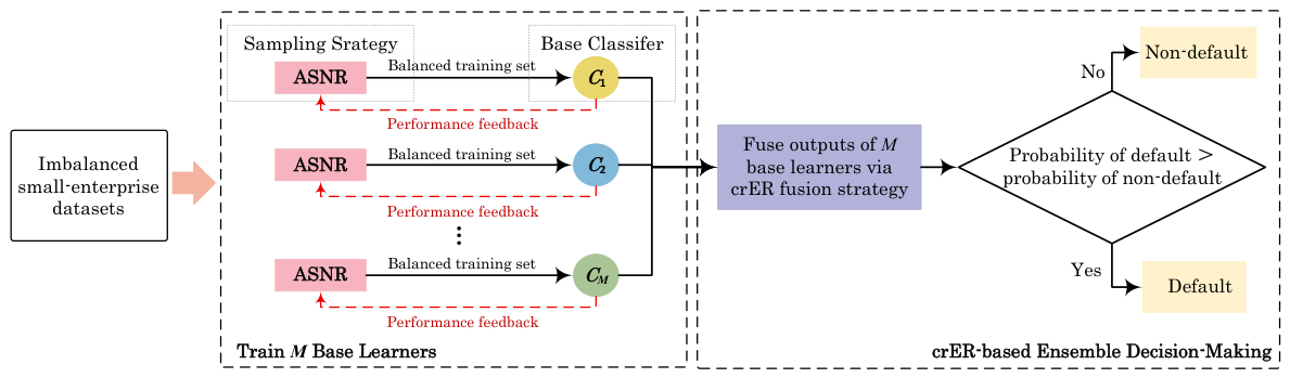
We propose the ASNR-crER model for imbalanced small-enterprise default risk prediction, and its overall framework is illustrated in Figure 1. The model follows an ensemble learning paradigm and consists of (M) base learners. Each base learner combines ASNR with a base classifier. For the (m)-th learner, ASNR first resamples the original imbalanced dataset to construct a balanced training set, which is then used to train classifier (C_m). During model training, the sampling parameters and classifier hyperparameters are jointly optimized under a unified validation criterion. In the ensemble stage, crER fuses the default and non-default probabilities generated by the (M) base learners. The final default status of each enterprise is determined by comparing the fused probabilities of the two classes.

3.1. Adaptive Spherical Neighborhood Resampling (ASNR)

3.1.1. SMOTE Principle and Research Motivation of ASNR

In standard SMOTE [49], a synthetic minority instance ${\tilde{x}}_j$ is generated by interpolating a minority seed instance $x_j$ and one of its k nearest minority neighbors $x_{i{l}^{\prime }}$:

$${\tilde{x}}_j=x_j+\lambda (x_{j{l}^{\prime }}-x_j),{\eta }_g\sim U(0,1),$$

(1)

where ${\eta }_g$ is a random coefficient sampled from a uniform distribution.

By repeating this interpolation, SMOTE expands the minority class to alleviate class imbalance. However, it implicitly assumes that all minority samples have equal sampling priority and that all indicators contribute equally to neighborhood construction and sample generation. These assumptions are restrictive in corporate default prediction. Default firms close to non-default firms are more likely to be misclassified, but they may be either informative boundary samples or harmful outliers. Outliers deviate from typical default patterns, and interpolating them may generate low-quality samples and expand erroneous decision regions. In contrast, boundary samples lie near the decision boundary and provide valuable information for boundary learning. Uniform sampling in SMOTE cannot distinguish between these two cases. Moreover, financial, non-financial, and macroeconomic indicators are often redundant and correlated, and their contributions to default identification differ. Treating them equally may weaken neighborhood characterization and reduce interpolation quality.

To address these limitations, the proposed ASNR extends SMOTE from two aspects. At the sample level, it identifies isolated default outliers and informative boundary samples according to the local neighborhood structure of default instances. It then assigns different sampling weights to boundary default samples. At the feature level, it embeds indicator importance into neighborhood construction and interpolation generation. In this way, key risk indicators play a larger role in synthetic sample generation.

3.1.2. Implementation Procedure of ASNR

The implementation of ASNR consists of five main steps.

Step 1: Indicator selection and weighting. LASSO and tree-based models are commonly used for indicator selection and weighting. Tree-based importance measures can evaluate variable contributions, but they usually provide rankings or importance scores rather than a naturally sparse indicator set [50]. LASSO performs indicator selection and coefficient estimation simultaneously [51], making it more suitable for constructing the weighted distance and guiding the interpolation process in ASNR.

Let the training set be $S_{\mathrm{train}}={\left\{(x_j,y_j)\right\}}_{j=1}^N$, where $x_j=(x_{j1},x_{j2},\dots ,x_{jp})$ represents the standardized vector of p candidate indicators for firm j, and $y_j\in \{0,1\}$ is its class label. LASSO is formulated as an $L_1$-regularized logistic regression model:

$$({\widehat{\beta }}_0,\widehat{\mathit{\beta }})=arg\underset{{\beta }_0,\mathit{\beta }}{min}\left[-{\displaystyle \frac{1}{N}}{\displaystyle \sum _{j=1}^N}\left\{y_{j}log{\rho }_j+(1-y_j)log(1-{\rho }_j)\right\}+\lambda {\displaystyle \sum _{i=1}^p}\left|{\beta }_i\right|\right],$$

(2)

where ${\rho }_j={\displaystyle \frac{1}{1+exp[-({\beta }_0+{\sum }_{i=1}^p{\beta }_i{x}_{ji})]}}$ is the estimated default probability of firm j in the LASSO logistic regression model. $\widehat{\beta }$ is the estimated coefficient vector, ${\widehat{\beta }}_0$ is the intercept term, and $\lambda$ is the regularization parameter. In this paper, the parameter $\lambda$ is determined by maximizing the AUC of the validation set. After substituting the optimal $\lambda$ into Equation (2), the final coefficient vector can be obtained. Assuming that LASSO retains u indicators, their nonzero coefficients are renumbered as $\widehat{\beta }=({\widehat{\beta }}_1,{\widehat{\beta }}_2,\dots ,{\widehat{\beta }}_u)$. Normalizing these coefficients yields the weight of the i-th indicator:

$${\omega }_i={\displaystyle \frac{log\left(\right|{\widehat{\beta }}_i|+1)}{{\sum }_{k=1}^{u}log\left(\right|{\widehat{\beta }}_k|+1)}},i=1,2,\dots ,u,$$

(3)

where ${\omega }_i\ge 0$ and ${\sum }_{i=1}^u{\omega }_i=1$. A larger ${\omega }_i$ reflects a higher contribution to default discrimination. The resulting weight vector $\omega =({\omega }_1,{\omega }_2,\dots ,{\omega }_u)$ is subsequently applied to the weighted distance calculation and feature-level interpolation.

Step 2: Adaptive spherical neighborhood construction. To accurately characterize the local feature space of default samples, ASNR constructs an adaptive spherical neighborhood for each default sample. Unlike the KNN neighborhoods used in most sampling methods, this approach determines its range via an adaptive distance threshold to better reflect local spatial density. Specifically, let $x_{ji}$ and $x_{li}$ denote the i-th indicator values for samples j and l, and ${\omega }_i$ represent the corresponding indicator weight. The similarity between any two samples is measured by the weighted Euclidean distance:

$$d(x_j,x_l)=\sqrt{\sum _{i=1}^u{\omega }_i{(x_{ji}-x_{li})}^2},$$

(4)

where a smaller $d(x_j,x_l)$ indicates that the two samples are more likely to be neighbors. Based on Equation (4), the pairwise distance matrix of the training set is computed as $D={\left[d(x_j,x_l)\right]}_{N\times N}$.

To define the neighborhood radius r, all positive pairwise weighted distances in D are sorted in ascending order, and the corresponding percentile is used as the radius. The percentile parameter $\tau$ is selected from the fixed candidate set $\mathcal{T}=\{0.05,0.10,0.15,\dots ,0.95\}$ by an exhaustive grid search. For each $\tau \in \mathcal{T}$, the radius $r\left(\tau \right)=Q_{\tau }\left(D\right)$ is used to construct spherical neighborhoods and generate a temporary resampled training set. The classifier is then trained on this resampled training set and evaluated on the validation set. The optimal percentile is determined by maximizing the validation AUC:

$${\tau }^{*}=arg\underset{\tau \in \mathcal{T}}{max}{\mathrm{AUC}}_{val}\left(\tau \right),r^{*}=Q_{{\tau }^{*}}\left(D\right).$$

(5)

Here, $Q_{{\tau }^{*}}\left(D\right)$ denotes the ${\tau }^{*}$-quantile of the pairwise distance matrix. The validation set is used only for selecting ${\tau }^{*}$, and the resampled training set generated under ${\tau }^{*}$ is retained for final model training.

Once $r$ is determined, any sample $x_l$ falling within $d(x_j^1,x_l)\le r$ is included in the spherical neighborhood of the j-th default sample $x_j^1$. Accordingly, the default-neighbor set $S_j^1$ and non-default-neighbor set $S_j^0$ are defined as

$$S_j^1=\left\{x_l\mid d(x_j^1,x_l)\le r,y_l=1,l\ne j\right\},$$

(6)

$$S_j^0=\left\{x_l\mid d(x_j^1,x_l)\le r,y_l=0,l\ne j\right\}.$$

(7)

Then, the full neighborhood of $x_j^1$ is defined as $S_j=S_j^1\cup S_j^0$.

Step 3: Identification of outlier, safe, and boundary samples. Based on the class composition of its spherical neighborhood, each default sample $x_j^1$ is classified into one of three types. If $\left|S_j^1\right|=0$, $x_j^1$ has no default neighbors and is treated as an outlier. It is assigned to $S_{\mathrm{outlier}}$ and excluded from subsequent oversampling to avoid generating synthetic samples from isolated default observations. If $|S_j^1|>0$ and $|S_j^0|=0$, $x_j^1$ is surrounded only by default samples and is regarded as a safe sample. It is assigned to $S_{\mathrm{safe}}$ and given a lower sampling priority. If $|S_j^1\left|\ge \right|S_j^0|>0$, $x_j^1$ lies near non-default samples and is regarded as a boundary sample. It is assigned to $S_{\mathrm{boundary}}$ and retained as a high-priority sampling seed.

Step 4: Sampling weight calculation based on local structure. In general, the informativeness of boundary samples varies with the local structure. Samples that are close to non-default instances and located in sparse default regions are more likely to be misclassified. However, they usually provide more useful information for shaping the decision boundary. Based on this idea, ASNR defines a contribution score for each boundary sample $x_j^1$ by combining relative distance and local class composition:

$$C_j={\displaystyle \frac{{min}_{x_{l^{\prime }}^1\in S_j^1}d(x_j^1,x_{l^{\prime }}^1)}{{min}_{x_{l^{\prime }}^1\in S_j^1}d(x_j^1,x_{l^{\prime }}^1)+{min}_{x_{h^{\prime }}^0\in S_j^0}d(x_j^1,x_{h^{\prime }}^0)+\epsilon }}+{\displaystyle \frac{|S_j^0|}{\left|S_j^1\right|+\left|S_j^0\right|}},x_j^1\in S_{\mathrm{boundary}},$$

(8)

where $\left(d(x_j^1,x_{l^{\prime }}^1)\right)$ denotes the distance from $\left(x_j^1\right)$ to its nearest default neighbor, and $\left(d(x_j^1,x_{h^{\prime }}^0)\right)$ denotes the distance from $\left(x_j^1\right)$ to its nearest non-default neighbor. The small constant $\left(\epsilon \right)$ is used to avoid division by zero. In the first term, the distance-based contribution is normalized by the sum of the nearest default and non-default distances, so that it reflects the relative position of $\left(x_j^1\right)$ around the boundary. This term becomes larger when $\left(x_j^1\right)$ is farther from default samples and closer to non-default samples. The second term is the local proportion of non-default samples and measures class overlap. Therefore, a larger $\left(C_j\right)$ indicates that the boundary sample is more informative and should receive higher sampling priority.

The sample-level sampling weight is obtained by normalizing the contribution scores over all boundary samples:

$${\pi }_j={\displaystyle \frac{C_j}{{\sum }_{x_j^1\in S_{\mathrm{boundary}}}{C}_j}},$$

(9)

where a larger ${\pi }_j$ indicates that more synthetic default samples are generated around $x_j^1$. It should be emphasized that the feature weights $\mathit{\omega }$ obtained in Step 1 directly affect the distance metric, thereby shaping the local neighborhood structure and sample distribution. This ultimately determines the sample-level sampling weight ${\pi }_j$. Such intrinsic coupling between feature-level weighting and sample-level allocation enables ASNR to focus on sparse boundary regions along key feature dimensions.

Step 5: Dual-weight guided synthetic sample generation. In the final stage, ASNR generates synthetic default samples using both the sample-level sampling weight ${\pi }_j$ and the indicator-level weight vector $\mathit{\omega }$. For each boundary default sample $x_j^1$, the number of synthetic samples is determined as

$$n_j=⌊{\pi }_j·\left(|S_{\mathrm{train}}^0\left|-\right|S_{\mathrm{train}}^1|\right)⌋,$$

(10)

where $|S_{\mathrm{train}}^0|$ and $|S_{\mathrm{train}}^1|$ denote the numbers of non-default and default samples in the training set, respectively, and $\lfloor ·\rfloor$ denotes the floor operator. Next, for each boundary sample $x_j^1$, ASNR randomly selects a default neighbor $x_{j{l}^{\prime }}^1$ and generates $n_j$ synthetic samples $x_{jg}^1$$(g=1,2,\dots ,n_j)$ through weighted interpolation:

$$x_{jg}^1=x_j^1+{\eta }_g\left[{\displaystyle \frac{(1_u+\omega )\odot (x_{j{l}^{\prime }}^1-x_j^1)}{1+{\omega }_{max}}}\right],{\eta }_g\sim U(0,1),$$

(11)

where $g=1,2,\dots ,n_j$, ${\omega }_{max}={max}_i{\omega }_i$, $1_u$ is an all-ones vector, and ⊙ denotes element-wise multiplication. The normalization term $1+{\omega }_{max}$ constrains the effective interpolation coefficient of the i-th indicator to ${\alpha }_{gi}={\eta }_g(1+{\omega }_i)/(1+{\omega }_{max})\in [0,1]$. Hence, each synthetic value lies within the interval defined by the corresponding feature values of $x_j^1$ and $x_{j{l}^{\prime }}^1$, preventing extrapolation beyond the segment between two default samples. The vector $\mathit{\omega }$ still gives more influential indicators relatively larger interpolation shifts, while the normalization constraint preserves valid interpolation.

According to Equation (11), ASNR traverses all boundary samples and generates $|S_{\mathrm{train}}^0\left|-\right|S_{\mathrm{train}}^1|$ synthetic default samples in total. These samples are then merged into the original training set to form a class-balanced resampled training set. The pseudocode of ASNR is presented in Algorithm 1.

3.1.3. Time Complexity Analysis

Indicator selection is a necessary preprocessing step in corporate default prediction. Although SMOTE, Borderline-SMOTE, and ADASYN are often assigned a complexity of $O\left(N^{2}u\right)$ [52], they also require feature selection in practice. For fairness, the LASSO-based selection and weighting in ASNR are treated as preprocessing, and the complexity analysis focuses only on resampling.

Given the training set $S_{\mathrm{train}}$, let N be the total number of samples. Let $N_0$ and $N_1$ denote the numbers of non-default and default samples, respectively, with $N_1\le N_0$. Assume that LASSO retains u indicators. For a single run of ASNR, computing the weighted pairwise distance matrix and determining the percentile-based radius requires $O(N^{2}u+N^{2}logN)$ time. Constructing spherical neighborhoods for default samples and identifying outlier, safe, and boundary samples requires $O\left(N_{1}N\right)$ time. Calculating the contribution scores and sampling weights of boundary samples requires $O\left(b\overline{s}\right)$ time, where b is the number of boundary samples and $\overline{s}$ is the average neighborhood size. Generating $G=N_0-N_1$ synthetic samples requires $O\left(Gu\right)$ time. Therefore, the total complexity of ASNR is $O(N^{2}u+N^{2}logN+N_{1}N+b\overline{s}+Gu)$. Since $b\le N_1\le N$, $\overline{s}\le N$, and $G\le N$, the overall complexity can be simplified to $O(N^{2}u+N^{2}logN)$.

Algorithm 1 Adaptive Spherical Neighborhood Resampling (ASNR)

1: Input: Training set $S_{\mathrm{train}}=S_{\mathrm{train}}^0\cup S_{\mathrm{train}}^1$, regularization parameter $\lambda$, the optimal quantile $\tau$, and small constant $\epsilon$   2: Output: Balanced training set $S_{\mathrm{train}}^b$   3: Fit the LASSO logistic model on $S_{\mathrm{train}}$ by Equation (2)   4: Retain u nonzero indicators and compute $\omega =({\omega }_1,{\omega }_2,\dots ,{\omega }_u)$ by Equation (3)   5: Compute the weighted pairwise distance matrix $D={\left[d(x_j,x_l)\right]}_{n\times n}$ by Equation (4)   6: Sort the nonzero distances in D in ascending order and set $r_{\tau }$ as the $\tau$-th percentile.   7: Initialize $S_{\mathrm{outlier}}$, $S_{\mathrm{safe}}$, $S_{\mathrm{boundary}}$, $S_j^{\mathrm{new}}$, and $S_{\mathrm{new}}$ as empty sets   8: for each default sample $x_j^1\in S_{\mathrm{train}}^1$ do   9:     Construct $S_j^1$ and $S_j^0$ by Equations (6) and (7) 10:     if $|S_j^1|=0$ then $S_{\mathrm{outlier}}\leftarrow S_{\mathrm{outlier}}\cup \left\{x_j^1\right\}$ 11:     else if $|S_j^1|>0\wedge |S_j^0|=0$ then $S_{\mathrm{safe}}\leftarrow S_{\mathrm{safe}}\cup \left\{x_j^1\right\}$ 12:     else if $|S_j^1\left|\ge \right|S_j^0|>0$ then $S_{\mathrm{boundary}}\leftarrow S_{\mathrm{boundary}}\cup \left\{x_j^1\right\}$ 13: end for 14: for each $x_j^1\in S_{\mathrm{boundary}}$ do 15:     Compute the number of synthetic samples $n_j$ by Equations (8)–(10) 16:     for $g=1$ to $n_j$ do 17:         Generate $x_{jg}^1$ by Equation (11), and update $S_j^{\mathrm{new}}\leftarrow S_j^{\mathrm{new}}\cup \left\{x_{jg}^1\right\}$ 18:     end for 19:     $S_{\mathrm{new}}\leftarrow S_{\mathrm{new}}\cup S_j^{\mathrm{new}}$ 20: end for 21: $S_{\mathrm{train}}^b\leftarrow S_{\mathrm{train}}^0\cup S_{\mathrm{safe}}\cup S_{\mathrm{boundary}}\cup S_{\mathrm{new}}$ 22: return $S_{\mathrm{train}}^b$

Compared with conventional SMOTE methods, ASNR is slightly more computationally expensive. This additional cost mainly arises from adaptive neighborhood construction and boundary weight calculation, but these steps help improve the selectivity and reliability of oversampling.

3.2. Class-Specific Reliability Evidential Reasoning Fusion (crER) for Ensemble Learning

3.2.1. Motivation and Rationale of crER

Most ensemble methods rely on majority voting or weighted voting to directly combine the classification results of base learners. Although these methods are easy to implement, they often ignore the confidence information contained in classifier outputs. Compared with discrete class labels, default probabilities provide a more informative representation of corporate risk levels. Moreover, base learners may differ not only in their overall predictive importance but also in their reliability in identifying default and non-default firms. Motivated by these considerations, this study introduces evidential reasoning theory and develops a class-specific reliability evidential reasoning fusion strategy, denoted as crER.

Yang and Singh [53] proposed evidential reasoning theory for uncertain multi-attribute decision-making. This theory represents multi-source judgments as belief distributions and combines them based on Dempster–Shafer (D–S) evidence theory. The classical D–S rule assumes that all evidence sources have equal importance and are fully reliable. To relax this assumption, Yang and Xu [54] further developed the ER rule by incorporating evidence weights and reliabilities into the recursive fusion process. Accordingly, when all evidence sources have equal weights and full reliability, the ER rule reduces to the classical D–S combination rule. Inspired by Cui et al. [55], who applied the ER rule to ensemble classification, this study further extends ER-based fusion by introducing class-specific reliability, leading to the proposed crER strategy. Unlike conventional ER-based fusion methods that usually assign a single reliability value to each evidence source, crER distinguishes the reliability of each base learner in recognizing default and non-default firms. In this way, the fusion process jointly considers learner importance, class probability confidence, and class-specific recognition reliability.

Table 2. Comparison of different ensemble and evidence fusion strategies.

Strategy	Decision Logic	Uncertainty Handling	Computational Cost	Interpretability
Majority voting	Aggregates hard class labels by simple vote counting.	–	Low	✓
Weighted voting	Aggregates hard labels or class probabilities using global learner weights.	–	Low	✓
Stacking	Learns a meta-decision function from base-learner outputs.	–	Medium	–
D–S combination rule	Maps base-learner outputs to basic belief assignments and combines them using the D–S rule.	✓	Low	✓
ER rule	Maps base-learner outputs into belief degrees and recursively fuses them by considering evidence importance and reliability.	✓	Low	✓
crER strategy	Maps base-learner outputs into belief degrees and recursively fuses them by considering each learner’s relative importance and class-specific reliability.	✓	Low	✓

Notes: ✓ denotes the presence of the corresponding property, whereas – denotes its absence or non-applicability.

summarizes the differences among common ensemble strategies and evidence fusion strategies in terms of decision logic, uncertainty handling, computational cost, and interpretability.

3.2.2. Implementation Procedure of crER

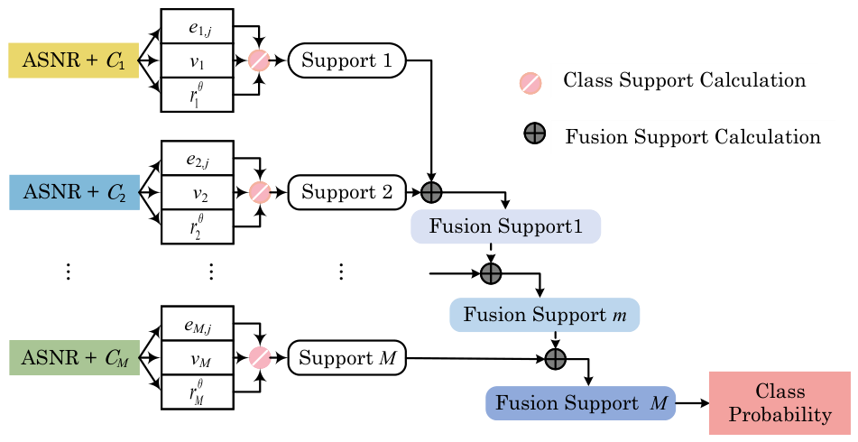
The workflow of crER is illustrated in Figure 2. First, each base learner generates an evidence unit $e_{m,j}$ for firm j. The evidence is then adjusted by the learner importance weight $v_m$ and the class-specific reliability $r_m^{\theta }$ to obtain class support degrees. Finally, the support degrees of different learners are recursively fused to generate the default and non-default probabilities of firm j. The detailed procedure is given in Steps 1–5.

Step 1: Estimate learner importance and class-specific reliability. Let $\{\mathrm{ASNR}-C_1,\mathrm{ASNR}-C_2,\dots ,\mathrm{ASNR}-C_M\}$ be an ensemble of M heterogeneous learners, where $C_m$ denotes the m-th classifier. The validation AUC is used to measure the global importance of each learner. The importance weight of learner m is defined as

$$v_m={\displaystyle \frac{{\mathrm{AUC}}_m}{{\sum }_{m=1}^M{\mathrm{AUC}}_m}},$$

(12)

where ${\mathrm{AUC}}_m$ is the validation AUC of learner m. AUC reflects the threshold-independent ranking and discrimination ability of a classifier. Therefore, it is suitable for measuring learner importance. The normalized weight satisfies ${\sum }_{m=1}^M{v}_m=1$, making the contributions of different learners comparable.

Since the predictive reliability of a learner may differ across classes, class-specific reliability is further introduced as

$$r_m^{\theta }=\left\{\begin{array}{cc}{\displaystyle \frac{{\mathrm{TP}}_m}{{\mathrm{TP}}_m+{\mathrm{FN}}_m},}\hfill & \theta =1,\hfill \\ {\displaystyle \frac{{\mathrm{TN}}_m}{{\mathrm{TN}}_m+{\mathrm{FP}}_m},}\hfill & \theta =0,\hfill \end{array}\right.$$

(13)

where ${\mathrm{TP}}_m$ and ${\mathrm{FN}}_m$ denote default firms that are correctly and incorrectly classified by learner m, respectively. Similarly, ${\mathrm{TN}}_m$ and ${\mathrm{FP}}_m$ denote non-default firms that are correctly and incorrectly classified by learner m, respectively. Thus, $r_m^1$ measures the reliability of learner m in identifying default firms, while $r_m^0$ measures its reliability in identifying non-default firms. These two measures correspond to recall and specificity. Compared with precision, they more directly describe class-wise correctness and are therefore more consistent with the purpose of class-specific reliability in crER.

Step 2: Construct evidence units. Let $\mathsf{\Phi }=\{1,0\}$ be the frame of discernment, where 1 denotes default and 0 denotes non-default. For firm j, the output of learner m is represented as the following evidence unit:

$$e_{m,j}=\left\{(\theta ,p_{m,j}^{\theta }),\theta \in \mathsf{\Phi },\sum _{\theta \in \mathsf{\Phi }}{p}_{m,j}^{\theta }=1\right\},$$

(14)

where $p_{m,j}^{\theta }$ is the probability mass assigned by learner m to class $\theta$ for firm j. For example, if the first learner assigns a default probability of $0.24$ to the first firm, the corresponding evidence unit is $e_{1,1}=\{(1,0.24),(0,0.76)\}$.

Step 3: Compute class support degrees. Given the learner importance, class-specific reliability, and evidence unit, the support degree assigned by learner m to class $\theta$ for firm j is calculated as

$$s_{m,j}^{\theta }=\left\{\begin{array}{cc}0,\hfill & \theta =\varnothing ,\hfill \\ {\tilde{v}}_m^{\theta }{p}_{m,j}^{\theta },\hfill & \theta \in \{1,0\},\hfill \\ {\displaystyle 1-\sum _{\theta \in \{1,0\}}{\tilde{v}}_m^{\theta }{p}_{m,j}^{\theta },}\hfill & \theta =\mathsf{\Phi },\hfill \end{array}\right.$$

(15)

where

$${\tilde{v}}_m^{\theta }={\displaystyle \frac{v_m}{1+v_m-r_m^{\theta }}}.$$

(16)

The null set receives zero support because it is not a feasible decision class. For $\theta \in \{1,0\}$, the predicted probability $p_{m,j}^{\theta }$ is discounted by ${\tilde{v}}_m^{\theta }$, which jointly reflects the global importance of learner m and its reliability for class $\theta$. A learner with stronger overall discrimination and higher class-specific reliability therefore provides greater support for the corresponding class. The remaining mass is assigned to $\mathsf{\Phi }$ and interpreted as residual uncertainty.

Step 4: Perform recursive evidence fusion. After the class support degrees and residual uncertainties of all learners are obtained, they are recursively fused to form a unified consensus. Let $s_{e(m-1),j}^{\theta }$ and $s_{e(m-1),j}^{\mathsf{\Phi }}$ denote the fused support for class $\theta$ and the residual uncertainty after combining the first $m-1$ learners, respectively. By incorporating the evidence of the m-th learner, the updated unnormalized support for firm j belonging to class $\theta$ is calculated as

$$\begin{array}{cc}\hfill {\widehat{s}}_{e\left(m\right),j}^{\theta }=& \left[(1-r_m^{\theta }),s_{e(m-1),j}^{\theta }+s_{e(m-1),j}^{\mathsf{\Phi }}{s}_{m,j}^{\theta }\right]+\sum _{A\cap B=\theta ;,A,B\subseteq \mathsf{\Phi }}{s}_{e(m-1),j}^A{s}_{m,j}^B,\hfill \end{array}$$

(17)

$$s_{e\left(m\right),j}^{\theta }={\displaystyle \frac{{\widehat{s}}_{e\left(m\right),j}^{\theta }}{{\sum }_{\theta \in 1,0}{\widehat{s}}_{e\left(m\right),j}^{\theta }+{\widehat{s}}_{e\left(m\right),j}^{\mathsf{\Phi }}}}.$$

(18)

In Equation (17), the term $(1-r_m^{\theta })s_{e(m-1),j}^{\theta }$ discounts the previously accumulated support according to the class-specific reliability of the incoming learner. The term $s_{e(m-1),j}^{\mathsf{\Phi }}{s}_{m,j}^{\theta }$ reallocates residual uncertainty to class $\theta$ based on the current learner’s support. The summation term increases ${\widehat{s}}_{e\left(m\right),j}^{\theta }$ only when the accumulated evidence and the incoming evidence are compatible with class $\theta$. When the two sources support different classes, their intersection is empty, and the corresponding conflicting mass is not assigned to either the default or non-default class. Instead, it is handled through the residual uncertainty term. After normalization, this uncertainty weakens the final class-specific support, thereby preventing conflicting evidence from being amplified into an overconfident decision. Finally, Equation (18) normalizes the fused class support and residual uncertainty to obtain the updated fused support.

Step 5: Obtain final class probabilities and prediction label. After all M learners are fused, Equation (19) normalizes the fused support degrees of the singleton classes to the interval $[0,1]$:

$$p_{e\left(M\right),j}^{\theta }={\displaystyle \frac{s_{e\left(M\right),j}^{\theta }}{{\displaystyle \sum _{{\theta }^{\prime }\in \{0,1\}}{s}_{e\left(M\right),j}^{{\theta }^{\prime }}}}},\theta \in \mathsf{\Phi }.$$

(19)

A larger $p_{e\left(M\right),j}^{\theta }$ indicates stronger fused evidence that firm j belongs to class $\theta$. Therefore, the final predicted label is determined by the class with the larger probability.

A complete numerical example with three base learners is provided in Appendix A. The pseudocode of crER is presented in Algorithm 2.

Algorithm 2 Class-specific Reliability Evidence Reasoning Fusion (crER)

1: Input: Balanced training sets ${\left\{S_{\mathrm{train}}^{b,m}\right\}}_{m=1}^M$, validation set $S_{\mathrm{val}}$, test set $S_{\mathrm{test}}$, classifier set $\{C_1,C_2,\dots ,C_M\}$, and class set $\mathsf{\Phi }=\{1,0\}$   2: Output: Predicted label ${\widehat{y}}_j$ for each firm j   3: for $m=1$ to M do   4:     Train and tune $C_m$ on $S_{\mathrm{train}}^{b,m}$ and $S_{\mathrm{val}}$ to obtain $C_m^{*}$   5:     Evaluate $C_m^{*}$ on $S_{\mathrm{val}}$ to obtain ${\mathrm{AUC}}_m$ and $\{{\mathrm{TP}}_m,{\mathrm{FN}}_m,{\mathrm{TN}}_m,{\mathrm{FP}}_m\}$   6: end for   7: Compute $v_m$ and $r_m^{\theta }$ for all learners using Equations (12) and (13)   8: for each firm $j\in S_{\mathrm{test}}$ do   9:     for $m=1$ to M do 10:         Predict $p_{m,j}^{\theta }$, construct $e_{m,j}$, and compute $s_{m,j}^{\theta }$ using Equations (14) and (15) 11:     end for 12:     Initialize $s_{e\left(1\right),j}^{\theta }\leftarrow s_{1,j}^{\theta }$ for $\theta \in \{1,0,\mathsf{\Phi }\}$ 13:     for $m=2$ to M do 14:         Recursively update $s_{e\left(m\right),j}^{\theta }$ using Equations (17) and (18) 15:     end for 16:     Compute $p_{e\left(M\right),j}^{\theta }$ using Equation (19) and set ${\widehat{y}}_j=arg{max}_{\theta \in \mathsf{\Phi }}{p}_{e\left(M\right),j}^{\theta }$ 17: end for 18: return ${\left\{{\widehat{y}}_j\right\}}_{j\in S_{\mathrm{test}}}$

3.3. Model Interpretability Based on SHAP

To explain our complex ensemble, we employ SHAP [56]. Unlike Gini importance or information gain, SHAP applies to any model class, yields exact feature attributions, and captures nonlinear effects. Let $\mathcal{F}$ be the full set of indicators, $\mathcal{U}\subseteq \mathcal{F}\setminus \left\{x_i\right\}$ be a subset excluding indicator $x_i$, and $C\left(\mathcal{U}\right)$ represent the model output when using $\mathcal{U}$. The Shapley value for indicator $x_i$ is defined as

$${\varphi }_i=\sum _{\mathcal{U}\subset \mathcal{F}\setminus \left\{x_i\right\}}\frac{\left|\mathcal{U}\right|!\left(\right|\mathcal{F}|-|\mathcal{U}|-1)!}{\left|\mathcal{F}\right|!}\left(C(\mathcal{U}\cup \left\{x_i\right\})-C\left(\mathcal{U}\right)\right).$$

(20)

where the combinatorial coefficient ${\displaystyle \frac{\left|\mathcal{U}\right|!\left(\right|\mathcal{F}|-|\mathcal{U}|-1)!}{\left|\mathcal{F}\right|!}}$ serves as a weighting factor, and $C(\mathcal{U}\cup \left\{x_i\right\})-C\left(\mathcal{U}\right)$ quantifies the incremental effect of $x_i$ on the model output. A larger ${\varphi }_i$ signifies a greater influence of $x_i$ on the prediction, and vice versa.

4. Experiment

4.1. Data

4.1.1. Data Description

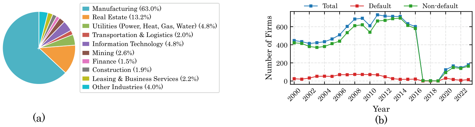
Our empirical analysis is based on data from Chinese listed small enterprises. The sample covers 10,449 firm-year observations from 2182 firms between 2000 and 2023. Figure 3a shows the industry distribution of the sample across 18 industries. The observations are mainly concentrated in manufacturing, real estate, and public utilities. This pattern is consistent with the industry distribution characteristics of Chinese listed small enterprises. Following Zhao et al. and Sun et al. [57,58], a firm is labeled as a default firm ($y=1$) if it is assigned ST or _*ST status by the stock exchange in the observed year. Otherwise, it is labeled as a non-default firm ($y=0$). Figure 3b presents the annual distribution of total observations, default observations, and non-default observations from 2000 to 2023. The results show that default events are rare during the sample period. This indicates a clear class imbalance problem in the data.

The initial indicator set contains 247 variables, including 153 financial indicators, 31 non-financial indicators, and 63 external macro-environmental indicators. The selection of indicators mainly follows prior studies on default prediction [30,58,59], while also considering data availability. Representative candidate indicators are reported in Appendix B,

Table A2. Representative candidate indicators for listed small enterprises.

Indicator Group	No. of Variables	Category	Representative Indicator
Financial indicators	153	Solvency	Liabilities/assets ratio
			Current liabilities/liabilities ratio
			Current ratio
			…
			Long-term debt ratio
			Other payables/current liabilities ratio
		Profitability	Earnings per share (basic)
			Earnings per share (deducted/basic)
			Book value per share
			…
			Annualized ROA
			Gross profit margin
		Operating capability	Cash operation index
			Cash recovery rate of total assets
			Current assets turnover ratio
			…
			Total asset turnover
			Working capital/total assets
		Growth capability	Book value per share growth rate
			Shareholders’ equity growth rate
			Capital preservation and appreciation rate
			…
			Total revenue growth rate
			Sustainable growth rate
Non-financial indicators	31	Shareholding structure	Top 3 shareholders’ combined stake
			Top 10 shareholders’ concentration index
			Top 10 shareholders Herfindahl index
			…
			Top 10 shareholders Z-index
			Top tradable shareholders H-index
		Corporate governance	Deficiency severity
			Deficiency rectification status
			Remedial measures taken
			…
			Audit opinion type
			Violation type
External macro-environmental indicators	63	Economic conditions	Industry prosperity index
			Macroeconomic prosperity index
			Annual entrepreneur confidence index
			…
			CPI index
			PPI index
		Consumption and income	Resident consumption level index
			Urban–rural consumption ratio index
			Urban household per capita income
			…
			Rural household per capita consumption
			Engel coefficient
		Investment and trade	Capital formation rate
			Capital formation growth rate
			Import–export growth rate
			…
			Freight turnover growth
			Domestic investment growth

Notes: This table reports representative candidate indicators selected from the 247 explanatory variables used in this study, including 153 financial indicators, 31 non-financial indicators, and 63 external macro-environmental indicators. Default status is the dependent variable and is not included among the candidate indicators. All indicators follow the standard definitions of the original authoritative data platforms.

. Due to space limitations, the table only lists representative variables from each indicator category. The financial indicators cover solvency, profitability, operating capability, and growth capability. The non-financial indicators include information on shareholding structure and corporate governance. The macro-environmental indicators mainly capture external conditions related to economic conditions, consumption and income, as well as investment and trade. All indicators follow the standard definitions of the original authoritative data platforms and are directly obtained from the following databases. Specifically, firm-level data are obtained from the Wind Financial Database (https://www.wind.com.cn/) and the CSMAR Database (https://data.csmar.com/). Macroeconomic data are obtained from the China Statistical Database (https://www.stats.gov.cn/english/Statisticaldata/, accessed on 20 June 2026).

4.1.2. Dataset Construction and Preprocessing

This paper constructs six prediction lead datasets, denoted as $t-m$, where $m=0,1,\dots ,5$. For each firm-year observation, the default status in year t is used as the label, while firm characteristics are traced back to year $t-m$. Therefore, the six datasets correspond to different prediction lead times and may share some firms, but they use different lagged feature years.

For each $t-m$ dataset, the training, validation, and test sets are divided chronologically according to the label year. All firm-year observations are first sorted by label year in ascending order. The label year is used as the minimum splitting unit, so observations from the same label year are assigned to the same subset. The split points are then selected to make the training, validation, and test sets as close as possible to a 7:2:1 ratio, while keeping their default rates relatively comparable. This strategy ensures that the training set contains earlier label years, the validation set contains subsequent label years, and the test set contains the latest label years. Thus, future default information is not used in model training or parameter tuning, which avoids look-ahead bias and temporal information leakage. The data-splitting results are reported in

Table 3. Statistics of small enterprises across different time windows and data splits.

Dataset	Total Observations (Firms)	Training Set (Default Rate)	Validation Set (Default Rate)	Testing Set (Default Rate)
t-0	10,449 (2182)	7314 (8.26%)	2090 (7.42%)	1045 (9.57%)
t-1	8263 (1732)	5784 (9.61%)	1652 (8.84%)	827 (9.43%)
t-2	6531 (1423)	4571 (10.65%)	1306 (11.26%)	654 (10.40%)
t-3	5108 (1150)	3575 (11.64%)	1022 (11.74%)	511 (13.31%)
t-4	3958 (906)	2770 (12.53%)	792 (14.14%)	396 (11.36%)
t-5	3052 (687)	2136 (13.39%)	606 (13.61%)	310 (11.76%)

. As shown in the table, the six datasets differ in the number of observations, number of firms, and default rates across the training, validation, and test sets.

Prior to modeling, each time-window dataset is preprocessed separately. The preprocessing procedures include: (1) calculating the mean and standard deviation of each continuous variable based only on the training set, and detecting and handling outliers using the three-sigma rule; (2) imputing missing values with the variable means calculated from the training set; and (3) applying min–max normalization to continuous variables using the minimum and maximum values estimated from the training set [30,60]. To avoid data leakage, the outlier thresholds, missing-value imputation statistics, and normalization parameters are all estimated only from the training set and then consistently applied to the validation and test sets.

4.2. Model Training and Tuning

As described in Section 3.1, ASNR starts with indicator selection and weighting. For each $t-m$ window, we employ the ${\ell }_1$-regularized Lasso logistic regression model defined in Equation (2) to select indicators and compute their weights. The numbers of retained indicators are 52, 48, 47, 39, 41, and 27 for the t-0, t-1, t-2, t-3, t-4, and t-5 windows, respectively. To illustrate the selection results,

Table 4. Lasso-selected indicators for t-2 dataset.

Criteria Layer	Indicator Name	${\widehat{\mathit{\beta }}}_{\mathit{i}}$	${\mathit{\omega }}_{\mathit{i}}$
Internal Financial Indicators	(1) Long-term debt ratio	1.591	0.026
	(2) Other receivables/current assets	1.088	0.025
	(3) Other payables/total current liabilities	−0.460	0.023
	(4) Return on human capital	−1.027	0.025
	(5) Return on total assets (annualized)	−3.453	0.028
	…	…	…
Internal Non-Financial Indicators	(24) Top 3 shareholders’ combined stake	−0.131	0.019
	(25) Top 10 shareholders H-index	−0.412	0.022
	(26) Top 10 tradable shares H-index	−0.924	0.025
	(27) Audit opinion type	1.448	0.026
	…	…	…
External Macroeconomic Indicators	(29) Entrepreneur confidence index (sector)	−0.146	0.019
	(30) Annual entrepreneur confidence index	−0.274	0.021
	(31) Total retail sales of consumer goods	−0.101	0.018
	(32) Resident consumption level index	−0.125	0.019
	(33) Commodity retail price index	0.428	0.023
	(34) Producer price index	0.015	0.013
	(47) Education expenditure growth rate	0.100	0.018

reports Lasso-selected indicators for the t-2 dataset, together with their estimated coefficients ${\widehat{\beta }}_i$ and normalized weights ${\omega }_i$.

Using the selected and weighted indicators as inputs, five representative classifiers are combined with ASNR to construct the base learners. Specifically, logistic regression (LR), support vector machine (SVM), Random Forest (RF), XGBoost, and LightGBM are used as base classifiers, forming ASNR-LR, ASNR-SVM, ASNR-RF, ASNR-XGB, and ASNR-LightGBM, respectively.

For each base learner, given a percentile parameter $\tau$, ASNR is applied only to the training set to generate synthetic default samples until the minority and majority classes are balanced. The corresponding classifier is then trained on the balanced training set. During training, the ASNR parameter $\tau$ and the classifier hyperparameters are jointly optimized through grid search, with the validation AUC used as the tuning criterion. The search range of $\tau$ is $\{0.05,0.10,\dots ,0.95\}$, and the search ranges of the classifier hyperparameters are provided in

Table 5. Classifier hyperparameters and their search ranges.

Classifier	Hyperparameter Search Range
LR	C: {0.001, 0.01, 0.1, 1, 10, 100}
SVM	C: {0.001, 0.01, 0.1, 1, 10, 100}; kernel: {linear, rbf}
RF	n_estimators: {20, 50, 100, 200, 300}; max_depth: {3, 4, 5, …, 10}
XGBoost, LightGBM	lr: {0.001, 0.01, 0.1, 1}; n_estimators: {20, 50, 100, 200, 300}; max_depth: {3, 4, 5, …, 10}

. After tuning, the probability outputs of the optimized base learners on the validation set are used to estimate the learner importance weights $v_m$ and the class-specific reliabilities $r_m^1$ and $r_m^0$ required by the crER fusion module. The final optimized configurations of ASNR-crER for all time windows are summarized in

Table 6. Parameter settings of ASNR-crER.

Dataset	Base Classifier (Best Params)	Weight ${\mathit{v}}_{\mathit{m}}$	Reliabilities ${\mathit{r}}_{\mathit{m}}^{\mathit{\theta }}$
			${\mathit{r}}_{\mathit{m}}^{\mathbf{1}}$	${\mathit{r}}_{\mathit{m}}^{\mathbf{0}}$
t-0	ASNR-LR: {$\tau$=0.80, C=100}	0.1984	0.8710	0.9023
	ASNR-SVM: {$\tau$=0.80, C=10, kernel=rbf}	0.1983	0.7097	0.9597
	ASNR-RF: {$\tau$=0.95, n_estimators=100, depth=8}	0.2012	0.8452	0.9235
	ASNR-XGBoost: {$\tau$=0.95, lr=0.01, n_estimators=100, depth=10}	0.2009	0.8258	0.9220
	ASNR-LightGBM: {$\tau$=0.95, lr=0.01, n_estimators=200, depth=7}	0.2012	0.8065	0.9313
t-1	ASNR-LR: {$\tau$=0.80, C=100}	0.1989	0.8562	0.9097
	ASNR-SVM: {$\tau$=0.80, C=10, kernel=rbf}	0.1988	0.8630	0.9057
	ASNR-RF: {$\tau$=0.80, n_estimators=200, depth=6}	0.2009	0.8562	0.9363
	ASNR-XGBoost: {$\tau$=0.95, lr=0.01, n_estimators=200, depth=5}	0.2004	0.8219	0.9602
	ASNR-LightGBM: {$\tau$=0.95, lr=0.1, n_estimators=200, max_depth=7}	0.2010	0.8425	0.9416
t-2	ASNR-LR: {$\tau$c=0.80, C=0.1}	0.2003	0.8299	0.8516
	ASNR-SVM: {$\tau$=0.80, C=10, kernel=linear}	0.2008	0.8027	0.8628
	ASNR-RF: {$\tau$=0.95, n_estimators=100, max_depth=10}	0.1992	0.8095	0.8801
	ASNR-XGBoost: {$\tau$=0.80, lr=0.01, n_estimators=200, max_depth=5}	0.2000	0.7891	0.8991
	ASNR-LightGBM: {$\tau$=0.95, lr=0.01, n_estimators=200, max_depth=8}	0.1997	0.6190	0.9422
t-3	ASNR-LR: {$\tau$=0.90, C=0.1}	0.2021	0.7917	0.7882
	ASNR-SVM: {$\tau$=0.50, C=0.1, kernel=rbf}	0.1983	0.7083	0.7971
	ASNR-RF: {$\tau$=0.50, n_estimators=200, max_depth=7}	0.2019	0.7333	0.8370
	ASNR-XGBoost: {$\tau$=0.80, lr=0.01, n_estimators=200, max_depth=10}	0.1983	0.7583	0.7838
	ASNR-LightGBM: {$\tau$=0.80, lr=0.1, n_estimators=200, max_depth=5}	0.1994	0.4083	0.9346
t-4	ASNR-LR: {$\tau$=0.95, C=0.01}	0.2005	0.6696	0.7706
	ASNR-SVM: {$\tau$=0.95, C=0.1, kernel=rbf}	0.2005	0.5893	0.8088
	ASNR-RF: {$\tau$=0.95, n_estimators=200, max_depth=3}	0.2016	0.7321	0.7500
	ASNR-XGBoost: {$\tau$=0.95, lr=0.01, n_estimators=100, max_depth=3}	0.2005	0.6875	0.7574
	ASNR-LightGBM: {$\tau$=0.95, lr=0.1, n_estimators=100, max_depth=8}	0.1969	0.2143	0.9485
t-5	ASNR-LR: {$\tau$=0.80, C=0.1}	0.2029	0.7349	0.7362
	ASNR-SVM: {$\tau$=0.80, C=0.1, kernel=linear}	0.2032	0.7349	0.7362
	ASNR-RF: {$\tau$=0.95, n_estimators=200, max_depth=5}	0.1963	0.4217	0.8899
	ASNR-XGBoost: {$\tau$=0.80, lr=0.01, n_estimators=100, max_depth=7}	0.1976	0.5663	0.7704
	ASNR-LightGBM: {$\tau$=0.80, lr=0.1, n_estimators=100, max_depth=5}	0.2001	0.3976	0.9108

.

4.3. Baseline Methods

To evaluate ASNR-crER, we compare it with benchmark methods from two perspectives: sampling strategies and credit prediction models. All experiments use the same data splits and feature inputs. Each setting is independently repeated 10 times, and the average performance is reported. For methods with tunable hyperparameters, models are trained on the training set, and the parameter setting with the highest validation AUC is selected by grid search.

The sampling methods compared in this study include random undersampling (RUS), SMOTE, Borderline-SMOTE, KMeans-SMOTE, SMOTE-WRND [41], HS-SMOTE [43], WGAN-GP [44], CTGAN [45], and TabDDPM [46]. To fairly assess the independent contribution of each sampling strategy, LightGBM v4.6.0 under Python 3.9.21 with the default implementation settings is used as the common classifier, and only the sampling method applied to the training set is varied. The proposed crER fusion module is not used in this comparison, thereby avoiding the additional influence of decision-level fusion and allowing the observed performance differences to be mainly attributed to the sampling strategies themselves. For tuning, the number of neighbors in SMOTE, Borderline-SMOTE, and SMOTE-WRND is searched over $\{2,3,4,5,6,7\}$; the number of clusters in KMeans-SMOTE is searched over $\{5,6,7,8,9,10\}$; and the boundary weight factor in HS-SMOTE is searched over $\{0.5,0.7,1.0,1.3,1.5\}$. For WGAN-GP, CTGAN, and TabDDPM, latent or hidden dimensions $\{32,64,128\}$, batch sizes $\{64,128\}$, and epochs $\{100,300\}$ are searched. For CTGAN, generator and discriminator dimensions are further searched over $\left\{\right(128,128),(256,256\left)\right\}$. RUS has no additional hyperparameters.

The credit prediction comparison includes two groups. The first contains traditional machine learning models and ASNR-based ensembles, including ASNR-RF, ASNR-XGBoost, ASNR-LightGBM, majority voting, weighted voting, and Stacking ensembles constructed from the five base classifiers in Table 5. The second contains existing imbalanced credit prediction methods, including EasyEnsemble [18], CE-gcForest [61], VAE-DF [62], SACN [63], and CUDF [33]. EasyEnsemble combines RUS with multiple base learners; LR, RF, SVM, and XGBoost are used here, with search ranges consistent with those in Table 5. CUDF is a confidence-based undersampling decision forest. Its number of random trees is searched over $\{20,50,100,150,300\}$, and the maximum depth is searched over $\{3,4,\dots ,10\}$. CE-gcForest and VAE-DF are improved gcForest models, introducing cost-sensitive learning and VAE-based oversampling, respectively. For both methods, the number of Random Forests per layer is searched over $\{400,600,800,1000,1200\}$, and the number of trees per forest is searched over $\{20,50,100,150,300\}$. SACN is a self-attention-based deep model, with network layers searched over $\{2,3,4\}$ and attention heads searched over $\{2,4,6\}$. For all baseline methods, no additional class weights or cost-sensitive strategies are introduced unless they are inherent to the original algorithm. Hyperparameters not explicitly mentioned follow the settings reported in the original literature.

4.4. Evaluation Metrics

To evaluate model performance on the imbalanced credit prediction dataset, we use five metrics: three classification metrics, accuracy (Acc), AUC, and F1-score, and two probability calibration metrics, the Brier scores for the default and non-default classes, denoted as BS¹ and BS⁰ [64].

Accuracy measures the overall proportion of correctly classified observations:

$$\mathrm{Acc}={\displaystyle \frac{TP+TN}{TP+TN+FP+FN}}.$$

(21)

AUC evaluates the model’s ability to distinguish default firms from non-default firms across all classification thresholds, with a larger value indicating stronger discrimination. The F1-score focuses on the positive class, namely default firms, and is suitable for imbalanced classification. It is defined as the harmonic mean of precision and recall:

$$\mathrm{F}1={\displaystyle \frac{2TP}{2TP+FP+FN}}.$$

(22)

BS¹ and BS⁰ measure the calibration of predicted probabilities for default and non-default firms, respectively, by computing the mean squared error between the predicted class probability and the true class membership:

$${\mathrm{BS}}^1={\displaystyle \frac{1}{n^1}}\sum _{j:y_j=1}{(1-p_j^1)}^2,$$

(23)

$${\mathrm{BS}}^0={\displaystyle \frac{1}{n^0}}\sum _{j:y_j=0}{(1-p_j^0)}^2,$$

(24)

where $y_j$ is the true label of firm j, $p_j^1$ and $p_j^0$ are the predicted probabilities of default and non-default, and $n^1$ and $n^0$ are the corresponding class sizes. Lower BS values indicate better calibration and more reliable predicted probabilities.

Computational efficiency is further evaluated using sampling time, training time, and the number of parameters (Params). Sampling time and training time are measured in seconds and denote the wall-clock time required for resampling and model fitting, respectively. The number of parameters serves as a proxy for model complexity, including trainable weights for neural networks, tree nodes for tree-based models, coefficients and intercepts for linear models, and total parameters across component models for ensemble methods.

5. Results and Analysis

5.1. Compare with Sampling Strategies

Table 7. Comparative performance of ASNR and baseline sampling strategies across six time windows (time refers to the start-to-end sampling duration; best values in bold).

Method	Dataset: t-0							Dataset: t-1
	Acc	AUC	F1	BS1	BS0	Time (s)	Params	Acc	AUC	F1	BS1	BS0	Time (s)	Params
Original	0.943	0.966	0.652	0.227	0.021	-	0	0.928	0.943	0.566	0.340	0.032	-	0
RUS	0.892	0.978	0.673	0.052	0.113	0.001	0	0.871	0.947	0.577	0.212	0.111	0.001	0
SMOTE	0.935	0.979	0.703	0.090	0.060	0.386	0	0.925	0.951	0.666	0.132	0.057	0.267	0
Borderline-SMOTE	0.936	0.979	0.732	0.110	0.058	0.668	0	0.933	0.949	0.685	0.110	0.044	0.481	0
KMeans-SMOTE	0.937	0.980	0.720	0.110	0.054	0.157	0	0.927	0.954	0.679	0.180	0.049	0.120	0
WGAN-GP [43]	0.943	0.962	0.687	0.220	0.037	98.969	17,269	0.936	0.942	0.629	0.374	0.052	90.398	16,753
CTGAN [44]	0.941	0.968	0.691	0.222	0.037	101.357	17,250	0.936	0.945	0.644	0.337	0.034	90.811	17,009
TabDDPM [45]	0.944	0.969	0.697	0.191	0.040	87.509	10,996	0.935	0.950	0.655	0.320	0.036	79.264	10,480
SMOTE-WRND [40]	0.939	0.975	0.689	0.120	0.039	4.136	0	0.931	0.949	0.673	0.124	0.045	2.713	0
HS-SMOTE [42]	0.937	0.970	0.704	0.116	0.045	1.630	0	0.933	0.952	0.670	0.137	0.054	1.434	0
ASNR (ours)	0.948	0.986	0.735	0.138	0.044	1.420	0	0.942	0.952	0.689	0.139	0.053	1.311	0
Method	Dataset: $\mathit{t}$-2							Dataset: $\mathit{t}$-3
	Acc	AUC	F1	BS1	BS0	Time (s)	Params	Acc	AUC	F1	BS1	BS0	Time (s)	Params
Original	0.926	0.913	0.455	0.297	0.052	-	0	0.858	0.826	0.331	0.499	0.056	-	0
RUS	0.858	0.902	0.543	0.070	0.156	0.002	0	0.760	0.822	0.469	0.174	0.216	0.001	0
SMOTE	0.917	0.903	0.618	0.203	0.082	0.180	0	0.863	0.838	0.480	0.326	0.106	0.068	0
Borderline-SMOTE	0.926	0.900	0.600	0.220	0.077	0.343	0	0.861	0.828	0.436	0.353	0.102	0.142	0
KMeans-SMOTE	0.922	0.902	0.622	0.213	0.076	0.084	0	0.864	0.838	0.461	0.345	0.100	0.054	0
WGAN-GP [43]	0.922	0.904	0.563	0.307	0.051	77.050	16,624	0.873	0.814	0.467	0.508	0.057	36.995	15,592
CTGAN [44]	0.925	0.905	0.554	0.309	0.052	66.720	16,880	0.875	0.815	0.473	0.506	0.064	41.628	15,848
TabDDPM [45]	0.920	0.909	0.604	0.270	0.056	61.207	10,351	0.876	0.834	0.469	0.469	0.064	40.198	9319
SMOTE-WRND [40]	0.927	0.897	0.599	0.215	0.064	1.768	0	0.874	0.822	0.467	0.481	0.103	0.909	0
HS-SMOTE [42]	0.924	0.905	0.590	0.250	0.062	1.245	0	0.876	0.825	0.482	0.436	0.078	0.768	0
ASNR (ours)	0.928	0.919	0.644	0.227	0.057	1.124	0	0.881	0.840	0.528	0.323	0.074	0.590	0
Method	Dataset: $\mathit{t}$-4							Dataset: $\mathit{t}$-5
	Acc	AUC	F1	BS1	BS0	Time (s)	Params	Acc	AUC	F1	BS1	BS0	Time (s)	Params
Original	0.817	0.777	0.144	0.410	0.081	-	0	0.814	0.818	0.166	0.240	0.152	-	0
RUS	0.689	0.815	0.280	0.063	0.243	0.001	0	0.647	0.827	0.350	0.223	0.321	0.001	0
SMOTE	0.809	0.811	0.372	0.238	0.130	0.047	0	0.775	0.816	0.364	0.300	0.210	0.023	0
Borderline-SMOTE	0.831	0.824	0.375	0.244	0.122	0.105	0	0.784	0.825	0.383	0.213	0.202	0.049	0
KMeans-SMOTE	0.811	0.839	0.375	0.241	0.123	0.043	0	0.776	0.799	0.352	0.329	0.207	0.032	0
WGAN-GP [43]	0.829	0.797	0.320	0.412	0.081	35.781	15,850	0.814	0.818	0.367	0.432	0.110	20.754	14,044
CTGAN [44]	0.828	0.783	0.339	0.406	0.084	32.490	16,106	0.807	0.804	0.342	0.434	0.110	19.494	14,300
TabDDPM [45]	0.827	0.780	0.242	0.389	0.094	29.169	9577	0.801	0.808	0.409	0.474	0.117	18.157	7771
SMOTE-WRND [40]	0.832	0.785	0.440	0.312	0.115	0.618	0	0.800	0.826	0.386	0.259	0.184	0.330	0
HS-SMOTE [42]	0.825	0.806	0.399	0.320	0.123	0.274	0	0.800	0.819	0.403	0.305	0.150	0.209	0
ASNR (ours)	0.835	0.836	0.464	0.258	0.110	0.300	0	0.821	0.829	0.458	0.263	0.113	0.217	0

compares ASNR with ten baseline sampling methods. Compared with the original imbalanced setting, ASNR improves accuracy, AUC, and F1 across all six time windows, with F1 gains ranging from 0.083 to 0.320. To provide an overall comparison,

Table 8. Average rankings of different sampling strategies across six time windows.

Method	Acc_Rank	AUC_Rank	F1_Rank	BS1_Rank	BS0_Rank	Overall
SMOTE Baselines
Original	5.167	6.833	10.500	8.500	1.833	6.567
RUS	9.500	5.000	8.667	2.167	10.000	7.067
SMOTE	8.167	4.333	4.833	3.000	9.000	5.867
Borderline-SMOTE	5.167	4.500	4.333	3.167	6.667	4.767
KMeans-SMOTE	6.833	3.833	4.500	4.500	6.833	5.300
SMOTE-WRND [40]	3.833	6.167	5.000	4.833	5.500	5.067
HS-SMOTE [42]	4.833	4.833	4.000	5.833	6.000	5.100
Deep Baselines
WGAN-GP [43]	3.667	7.667	7.500	10.000	2.333	6.233
CTGAN [44]	3.500	7.500	7.333	9.667	2.000	6.000
TabDDPM [45]	4.000	5.833	5.500	8.167	3.167	5.333
Our Method
ASNR	1.000	1.333	1.000	4.833	4.500	2.533

reports the average rankings of different methods in terms of accuracy, AUC, F1, BS¹, and BS⁰, where a lower value indicates better performance. ASNR ranks first in accuracy, AUC, and F1, with average ranks of 1.000, 1.333, and 1.000, respectively. Its overall rank is 2.533, the best among all methods. These results show that ASNR improves both overall prediction accuracy and default sample identification.

For probability calibration, ASNR does not achieve the lowest Brier score for both classes, but its calibration remains relatively balanced between default and non-default firms. This suggests that ASNR improves classification performance without introducing a clear class bias. In contrast, Original and RUS obtain low Brier scores for one class but perform less favorably for the other, indicating stronger inter-class calibration imbalance. Deep generative methods, including WGAN-GP, CTGAN, and TabDDPM, generally show better calibration for the non-default class than for the default class. This may be because default samples are rare and heterogeneous, making it difficult for these models to learn a representative minority-class distribution. Overall, the balanced training samples constructed by ASNR enhance classification performance while maintaining relatively balanced probability calibration.

Table 7 also reports the sampling time and parameter scale of different sampling strategies. ASNR requires a sampling time comparable to SMOTE-based methods and much shorter than deep generative methods. In terms of parameter scale, SMOTE-based methods and ASNR are non-parametric geometric interpolation methods with no trainable parameters, whereas deep generative methods rely on neural networks with thousands of parameters. Overall, ASNR reconstructs the minority-class distribution more effectively while maintaining low computational cost and practical applicability, providing useful data-level support for early high-risk firm identification and risk-capital allocation.

5.2. Comparisons with Imbalanced Credit Prediction Models

Table 9. Comparative performance of ASNR-crER and baseline methods across six time windows (time refers to the model-fitting duration; best values in bold).

Method	Dataset: t-0							Dataset: t-1
	Acc	AUC	F1	BS1	BS0	Time (s)	Params	Acc	AUC	F1	BS1	BS0	Time (s)	Params
EasyEnsemble [59]	0.937	0.974	0.723	0.199	0.053	1.136	643	0.940	0.934	0.702	0.223	0.033	1.047	623
CUDF [63]	0.946	0.942	0.716	0.335	0.016	1.422	8125	0.952	0.940	0.726	0.241	0.023	1.340	7492
CE-gcForest [60]	0.951	0.967	0.741	0.257	0.025	1.446	178,270	0.952	0.940	0.726	0.241	0.023	1.357	161,412
VAE-DF [61]	0.952	0.972	0.719	0.244	0.016	1.883	197,237	0.944	0.943	0.705	0.248	0.028	2.007	172,286
SACN [62]	0.946	0.960	0.708	0.253	0.020	1.441	158,305	0.954	0.927	0.740	0.244	0.019	1.351	155,478
ASNR-RF	0.934	0.972	0.721	0.108	0.044	1.422	8125	0.924	0.938	0.677	0.147	0.047	1.341	7492
ASNR-XGBoost	0.928	0.969	0.704	0.097	0.052	1.557	1491	0.921	0.934	0.663	0.148	0.050	1.376	1488
ASNR-LightGBM	0.950	0.976	0.735	0.205	0.019	1.515	1274	0.954	0.940	0.743	0.235	0.018	1.374	1278
ASNR-Majority Vote	0.937	0.902	0.723	0.140	0.055	2.114	10,808	0.940	0.886	0.719	0.179	0.048	1.525	10,156
ASNR-Weighted Vote	0.940	0.976	0.725	0.112	0.035	2.114	10,808	0.941	0.936	0.717	0.168	0.037	1.525	10,156
ASNR-Stacking (LR)	0.922	0.976	0.692	0.058	0.061	2.114	10,814	0.917	0.939	0.667	0.106	0.062	1.525	10,162
ASNR-Stacking (XGB)	0.946	0.949	0.711	0.266	0.020	2.137	12,246	0.946	0.919	0.710	0.252	0.025	1.532	11,582
ASNR-crER (Ours)	0.955	0.977	0.769	0.158	0.022	2.114	10,823	0.955	0.945	0.758	0.191	0.020	1.525	10,171
Method	Dataset: $\mathit{t}$-2							Dataset: $\mathit{t}$-3
	Acc	AUC	F1	BS1	BS0	Time (s)	Params	Acc	AUC	F1	BS1	BS0	Time (s)	Params
EasyEnsemble [59]	0.913	0.900	0.629	0.185	0.055	0.922	603	0.797	0.841	0.464	0.194	0.148	0.056	598
CUDF [63]	0.917	0.908	0.640	0.231	0.048	1.111	8441	0.847	0.851	0.494	0.280	0.079	0.108	7378
CE-gcForest [60]	0.925	0.908	0.620	0.342	0.026	1.139	173,019	0.853	0.840	0.510	0.384	0.076	0.274	143,634
VAE-DF [61]	0.913	0.907	0.623	0.223	0.054	1.785	181,874	0.853	0.850	0.503	0.289	0.075	15.616	151,443
SACN [62]	0.907	0.911	0.612	0.179	0.080	1.136	142,305	0.863	0.850	0.493	0.306	0.067	0.211	102,305
ASNR-RF	0.914	0.905	0.636	0.227	0.057	1.120	7441	0.867	0.826	0.514	0.323	0.074	0.003	7378
ASNR-XGBoost	0.881	0.896	0.546	0.218	0.074	1.170	1490	0.875	0.852	0.484	0.382	0.046	0.261	1496
ASNR-LightGBM	0.930	0.910	0.652	0.339	0.022	1.136	1154	0.834	0.767	0.520	0.324	0.142	0.097	1078
ASNR-Majority Vote	0.905	0.824	0.613	0.279	0.073	1.322	11,103	0.855	0.852	0.543	0.254	0.090	1.070	10,022
ASNR-Weighted Vote	0.904	0.908	0.599	0.201	0.061	1.322	11,103	0.797	0.852	0.500	0.169	0.143	1.170	10,022
ASNR-Stacking (LR)	0.879	0.906	0.578	0.150	0.091	1.322	11,109	0.849	0.739	0.342	0.628	0.053	1.045	10,028
ASNR-Stacking (XGB)	0.917	0.872	0.591	0.373	0.038	1.329	12,522	0.812	0.829	0.495	0.245	0.115	1.051	11,451
ASNR-crER (Ours)	0.928	0.911	0.652	0.276	0.030	1.322	11,118	0.877	0.854	0.526	0.303	0.041	1.070	10,037
Method	Dataset: $\mathit{t}$-4							Dataset: $\mathit{t}$-5
	Acc	AUC	F1	BS1	BS0	Time (s)	Params	Acc	AUC	F1	BS1	BS0	Time (s)	Params
EasyEnsemble [59]	0.806	0.834	0.483	0.156	0.179	0.052	600	0.810	0.834	0.463	0.256	0.107	0.002	595
CUDF [63]	0.881	0.845	0.505	0.366	0.067	0.070	8486	0.807	0.814	0.427	0.282	0.104	0.024	6310
CE-gcForest [60]	0.842	0.845	0.484	0.228	0.125	0.905	163,702	0.866	0.844	0.453	0.340	0.068	0.064	119,540
VAE-DF [61]	0.855	0.834	0.422	0.351	0.069	1.386	177,305	0.807	0.814	0.427	0.282	0.104	0.731	131,341
SACN [62]	0.871	0.835	0.485	0.297	0.078	0.907	2305	0.827	0.838	0.405	0.283	0.090	0.014	87,552
ASNR-RF	0.821	0.822	0.450	0.258	0.113	0.900	128,255	0.807	0.815	0.459	0.263	0.113	0.056	6310
ASNR-XGBoost	0.869	0.822	0.480	0.365	0.072	0.906	1496	0.830	0.845	0.409	0.303	0.081	0.016	1497
ASNR-LightGBM	0.889	0.825	0.463	0.448	0.035	0.906	1180	0.886	0.846	0.444	0.475	0.042	0.024	949
ASNR-Majority Vote	0.866	0.750	0.505	0.400	0.100	0.936	11,122	0.837	0.739	0.468	0.389	0.133	0.083	8899
ASNR-Weighted Vote	0.881	0.846	0.505	0.305	0.067	0.936	11,122	0.846	0.851	0.447	0.291	0.081	0.083	8899
ASNR-Stacking (LR)	0.742	0.834	0.427	0.147	0.182	0.936	11,128	0.716	0.830	0.416	0.129	0.205	0.083	8905
ASNR-Stacking (XGB)	0.843	0.744	0.311	0.574	0.068	0.936	12,561	0.843	0.779	0.351	0.544	0.073	0.084	10,321
ASNR-crER (Ours)	0.894	0.850	0.512	0.363	0.043	0.936	11,137	0.892	0.854	0.522	0.300	0.063	0.083	8914

benchmarks ASNR-crER against 12 imbalanced credit prediction models, including representative imbalanced learning methods and ASNR-based variants. ASNR-crER achieves the highest AUC across all six prediction windows and obtains the best Acc and F1-scores in five windows. Although its Acc in the t-2 window is 0.002 lower than ASNR-LightGBM and its F1 in the t-3 window is 0.017 lower than ASNR-Majority Vote, these small gaps do not affect its overall advantage.

Table 10. Average rankings of imbalanced credit prediction models across six time windows.

Method	Acc_Rank	AUC_Rank	F1_Rank	BS1_Rank	BS0_Rank	Overall
Ensemble baseline
EasyEnsemble [59]	9.667	7.833	7.000	3.833	10.167	7.700
CUDF [63]	6.000	6.333	5.833	8.167	4.833	6.233
Deep baselines
CE-gcForest [60]	4.833	6.000	4.833	9.500	5.667	6.167
VAE-DF [61]	6.833	6.333	8.167	7.333	5.833	6.900
SACN [62]	5.667	6.667	8.333	7.000	6.333	6.800
ASNR-based baselines
ASNR-RF	8.667	9.000	6.667	4.6667	8.833	7.567
ASNR-XGBoost	8.500	7.333	11.333	6.5000	8.000	8.333
ASNR-LightGBM	3.500	5.667	4.333	10.1667	3.000	5.333
ASNR-Majority Vote	7.667	11.167	4.333	7.6667	10.500	8.267
ASNR-Weighted Vote	7.667	4.000	6.000	4.3333	7.833	5.967
ASNR-Stacking (LR)	12.167	7.167	11.833	3.0000	11.333	9.100
ASNR-Stacking (XGB)	6.667	11.667	10.500	11.1667	5.500	9.100
Our method
ASNR-crER	1.167	1.000	1.167	7.333	2.833	2.700

further reports the average rankings of all models across the six time windows. ASNR-crER obtains the best overall rank of 2.700, followed by ASNR-LightGBM, ASNR-Weighted Vote, and CE-gcForest, with average ranks of 5.333, 5.967, and 6.167, respectively. The strong performance of ASNR-LightGBM and ASNR-Weighted Vote confirms the effectiveness of ASNR in reconstructing minority-class distributions. More importantly, ASNR-crER further improves prediction stability by incorporating class-specific reliability into recursive evidential fusion. Compared with deep baseline models, ASNR-crER also achieves a better balance between predictive performance and model complexity. For example, CE-gcForest uses a deep cascade ensemble with 119,540 to 178,270 parameters across the six windows, whereas ASNR-crER uses only 8914 to 11,137 parameters while achieving the best overall ranking. This suggests that ASNR-crER improves credit prediction through adaptive resampling and reliable evidence fusion rather than excessive model complexity. Although ASNR-crER requires slightly longer training time than some single-model baselines because it trains multiple base learners and performs evidential fusion, the additional time cost is marginal.

Taken together, Table 9 and Table 10 show that ASNR-crER maintains stable predictive advantages across different prediction horizons. Because these windows differ in sample size, class-imbalance degree, and selected feature subsets, the results also demonstrate the robustness of ASNR-crER under varying data distributions and feature spaces. This multi-window performance helps financial institutions identify high-risk firms at different stages of credit exposure and supports more dynamic credit risk management.

5.3. Significance Test

The comparative experiments show that the proposed methods achieve clear advantages in accuracy (Acc), AUC, and F1. When default samples are scarce, however, higher F1-scores may partly reflect sample fluctuation rather than stable improvement. Therefore, this section conducts one-sided paired t-tests on the F1-scores from 10 independent runs. After verifying that the paired F1-score differences approximately follow a normal distribution, the null hypothesis is defined as the proposed method having a mean F1-score no higher than that of the corresponding baseline, while the alternative hypothesis assumes a significantly higher mean F1-score. Significance is evaluated at the 10%, 5%, and 1% levels, denoted by *, **, and ***, respectively.

Table 11. Results of paired t-tests on F1-scores between ASNR and baseline methods across different time windows.

ASNR vs.	t-0	t-1	t-2	t-3	t-4	t-5
Original	4.679 *** (0.0012)	10.497 *** (0.0000)	15.258 *** (0.0000)	9.131 *** (0.0000)	16.235 *** (0.0000)	9.493 *** (0.0000)
RUS	3.190 ** (0.0110)	9.379 *** (0.0000)	19.378 *** (0.0000)	4.788 *** (0.0010)	20.722 *** (0.0000)	8.611 *** (0.0000)
SMOTE	1.937 * (0.0847)	2.291 ** (0.0477)	1.984 * (0.0785)	2.487 ** (0.0346)	4.673 *** (0.0012)	4.414 *** (0.0017)
Borderline-SMOTE	0.181 (0.8604)	0.402 (0.6971)	2.822 ** (0.0200)	8.123 *** (0.0000)	4.680 *** (0.0012)	3.683 *** (0.0051)
WGAN-GP [43]	3.558 *** (0.0061)	3.966 *** (0.0033)	3.861 *** (0.0038)	2.685 ** (0.0250)	12.332 *** (0.0000)	3.301 *** (0.0092)
CTGAN [44]	2.685 ** (0.0250)	3.049 ** (0.0138)	5.814 *** (0.0003)	4.027 *** (0.0030)	5.015 *** (0.0007)	5.281 *** (0.0005)
TabDDPM [45]	2.700 ** (0.0244)	2.710 ** (0.0240)	3.714 *** (0.0048)	9.558 *** (0.0000)	11.140 *** (0.0000)	1.906 * (0.0890)
SMOTE-WRND [40]	1.822 (0.1017)	1.026 (0.3316)	3.796 *** (0.0042)	3.790 *** (0.0043)	1.145 (0.2818)	3.204 ** (0.0108)
HS-SMOTE [42]	1.877 * (0.0932)	0.998 (0.3442)	3.768 *** (0.0044)	3.148 ** (0.0118)	3.886 *** (0.0037)	2.056 * (0.0699)

Notes: Each cell reports the paired one-sided t-statistic, with the corresponding p-value in parentheses. *, **, and *** indicate significance at the 10%, 5%, and 1% levels, respectively.

reports the paired t-test results between ASNR and the sampling baselines. ASNR significantly outperforms Original, RUS, and SMOTE across all six time windows. Compared with Borderline-SMOTE, SMOTE-WRND, and HS-SMOTE, ASNR does not show significant advantages in every window, but most results still support its improvement, especially in medium- and long-horizon windows. Compared with WGAN-GP, CTGAN, and TabDDPM, ASNR achieves significant gains in almost all cases, suggesting that geometric sample reconstruction is more stable than deep generative sampling for tabular credit prediction with scarce default samples.

Table 12. Results of paired t-tests on F1-scores between ASNR-crER and competing methods across different time windows.

Comparison	t-0	t-1	t-2	t-3	t-4	t-5
EasyEnsemble [61]	7.332 *** (0.0000)	7.946 *** (0.0000)	4.297 *** (0.0010)	7.557 *** (0.0000)	3.501 *** (0.0034)	7.436 *** (0.0000)
CUDF [63]	7.016 *** (0.0000)	3.921 *** (0.0018)	1.838 ** (0.0496)	4.188 *** (0.0012)	0.617 (0.2762)	7.328 *** (0.0000)
CE-gcForest [62]	5.630 *** (0.0002)	6.634 *** (0.0000)	3.580 *** (0.0030)	1.581 * (0.0741)	1.913 ** (0.0440)	3.399 *** (0.0039)
VAE-DF [63]	5.760 *** (0.0001)	7.859 *** (0.0000)	3.009 *** (0.0074)	3.363 *** (0.0042)	8.029 *** (0.0000)	10.267 *** (0.0000)
SACN [64]	8.375 *** (0.0000)	2.199 ** (0.0277)	4.294 *** (0.0010)	4.633 *** (0.0006)	2.558 ** (0.0154)	15.904 *** (0.0000)
ASNR-RF	6.353 *** (0.0001)	9.888 *** (0.0000)	2.456 ** (0.0182)	1.520 * (0.0814)	5.467 *** (0.0002)	4.860 *** (0.0004)
ASNR-XGBoost	18.157 *** (0.0000)	20.018 *** (0.0000)	24.482 *** (0.0000)	8.554 *** (0.0000)	5.936 *** (0.0001)	15.299 *** (0.0000)
ASNR-LightGBM	8.744 *** (0.0000)	3.721 *** (0.0024)	0.060 (0.4768)	0.988 (0.1745)	8.346 *** (0.0000)	10.442 *** (0.0000)
ASNR-Majority Vote	8.470 *** (0.0000)	6.688 *** (0.0000)	8.731 *** (0.0000)	−3.539 (0.9968)	1.142 (0.1415)	6.597 *** (0.0000)
ASNR-Weighted Vote	14.303 *** (0.0000)	8.274 *** (0.0000)	9.729 *** (0.0000)	4.523 *** (0.0007)	1.776 * (0.0547)	12.422 *** (0.0000)
ASNR-Stacking (LR)	9.436 *** (0.0000)	13.417 *** (0.0000)	11.190 *** (0.0000)	12.624 *** (0.0000)	3.426 *** (0.0038)	6.250 *** (0.0001)
ASNR-Stacking (XGB)	15.200 *** (0.0000)	4.288 *** (0.0010)	6.140 *** (0.0001)	2.403 ** (0.0198)	10.827 *** (0.0000)	10.096 *** (0.0000)

Notes: Each cell reports the paired one-sided t-statistic, with the corresponding p-value in parentheses. *, **, and *** indicate significance at the 10%, 5%, and 1% levels, respectively.

reports the paired t-test results between ASNR-crER and competing credit prediction models. ASNR-crER achieves significant F1 improvements over most baselines across the six time windows. Although its advantages over ASNR-LightGBM, ASNR-Majority Vote, and CUDF are not significant in some windows, most corresponding t-statistics remain positive, indicating that the results generally favor ASNR-crER. Overall, these tests suggest that the performance gains of ASNR-crER are not mainly driven by random fluctuations.

5.4. Robustness Analysis

5.4.1. Performance Evaluation and Stability Under Concept Drift

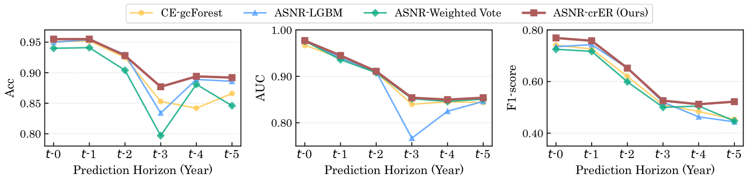
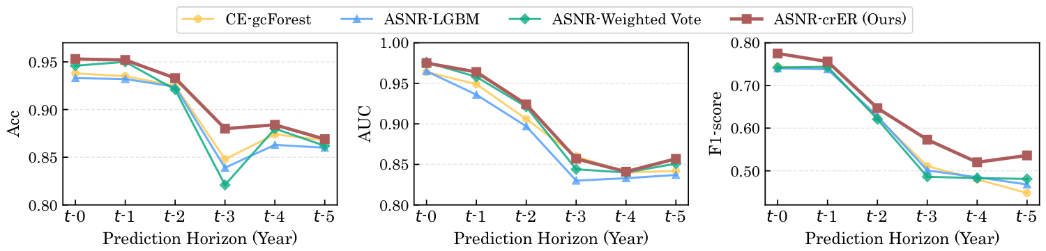
Model stability under potential concept drift is examined by tracking ASNR-crER and the three strongest baselines identified in Table 9 across six prediction windows (t-0 to t-5). The results are shown in Figure 4. All models perform well in the short-term windows (t-0 and t-1). As the prediction horizon lengthens, accuracy, AUC, and F1-score gradually decline, with a sharper drop around t-3 and a relatively stable trend thereafter. This pattern suggests that the discriminatory information in default-related indicators weakens over longer horizons. Despite this decline, ASNR-crER maintains a stable comparative advantage across all windows.

To quantify temporal robustness, we calculate the performance decay rate of each metric as $(M_{t0}-M_{tk})/M_{t0}\times 100\%$, where $M_{t0}$ denotes the performance at t-0 and $M_{tk}$ denotes the performance at window t-k$(k=1,\dots ,5)$. The maximum, minimum, and average decay rates are reported in

Table 13. Performance decay statistics of representative models across prediction windows.

Method	Acc Decay Rate			AUC Decay Rate			F1 Decay Rate
	Max	Min	Avg	Max	Min	Avg	Max	Min	Avg
CE-gcForest	11.46%	−0.11%	6.67%	13.13%	2.79%	9.47%	38.87%	2.02%	24.62%
ASNR-LightGBM	12.21%	−0.42%	5.41%	21.41%	3.69%	12.13%	39.59%	−1.09%	23.21%
ASNR-Weighted Vote	15.21%	−0.11%	7.04%	13.32%	4.10%	9.98%	38.34%	1.10%	23.64%
ASNR-crER (Ours)	8.17%	0.00%	4.80%	13.00%	3.28%	9.64%	33.42%	1.43%	22.76%

. ASNR-crER achieves the lowest maximum and average decay rates in both accuracy and F1-score, with average decay rates of 4.80% and 22.76%, respectively, outperforming CE-gcForest, ASNR-LightGBM, and ASNR-Weighted Vote. Although CE-gcForest shows a slightly smaller AUC decay, its F1-score drops more sharply, indicating faster deterioration in long-horizon default identification. In contrast, ASNR-crER maintains more stable minority-class recognition as the prediction horizon increases.

5.4.2. Robustness Analysis with an Extended Sample Period

Previous experiments have shown the advantages of ASNR-crER in multi-window corporate default prediction. A key practical concern is whether the model remains effective as firm-year observations are updated. To examine this issue, we incorporate newly available 2024–2025 observations for an extended sample robustness test. The data were collected from the same sources described in Section 4.1. Following the same screening criteria, firms listed for fewer than two years and those with more than 20% missing indicators were excluded, yielding 268 valid firm-year observations, including 36 default and 232 non-default observations. Using the default status in 2024 and 2025 as labels, we traced back the corresponding indicators and constructed extended samples for six prediction windows from t-0 to t-5. These observations were then merged into the original test sets to evaluate the temporal extrapolation stability of the trained models.

Figure 5 reports the extended sample robustness results. After incorporating the 2024–2025 observations, ASNR-crER still achieves the best overall performance. Across most prediction windows, it obtains higher or highly competitive accuracy, AUC, and F1-scores than the benchmark models. This indicates that ASNR-crER retains strong classification, risk-ranking, and minority default identification abilities under the extended sample setting, showing temporal extrapolation stability when corporate observations are continuously updated.

5.5. Effectiveness Analysis of ASNR and crER Modules

To examine the effectiveness of ASNR-crER, we conduct ablation experiments and internal mechanism analysis on the t-2 dataset. The t-2 window is commonly used in single-window default prediction for listed firms, as it provides early-warning signals two years before default while preserving the reliability of financial information.

5.5.1. Ablation Study of ASNR-crER

Table 14. Ablation results of ASNR-crER.

Setting	ASNR	crER	Acc	AUC	F1
w/o crER	✓	–	0.905 6.137 (0.0001) ***	0.824 78.586 (0.0000) ***	0.613 3.044 (0.0070) ***
w/o ASNR	–	✓	0.926 1.438 (0.0921) *	0.900 9.165 (0.0000) ***	0.547 6.822 (0.0000) ***
ASNR-crER (Ours)	✓	✓	0.928	0.911	0.652

Notes: The symbol ✓ indicates that the corresponding module is used, whereas – indicates that it is removed. The first line in each metric cell reports the mean performance value. The second line reports the paired one-sided t-test statistic and the corresponding p-value in parentheses, comparing ASNR-crER with the ablated variant. * and *** indicate significance at the 10% and 1% levels, respectively.

reports the ablation results of ASNR and crER. A paired one-sided t-test is further used to examine whether the complete ASNR-crER model significantly outperforms its ablated variants. When crER is removed and replaced with majority voting, Acc, AUC, and F1 decrease by 0.023, 0.087, and 0.039, respectively. The improvements of the complete model are all significant at the 1% level, indicating that crER more effectively integrates base-learner outputs through class-specific reliability modeling and recursive evidential fusion. When ASNR is removed and crER is directly applied to the original imbalanced data, Acc, AUC, and F1 decrease by 0.002, 0.011, and 0.105, respectively. The improvement in Acc is significant at the 10% level, while those in AUC and F1 are significant at the 1% level. The substantial decline in F1 shows that insufficient minority-class information limits the ability of decision-level fusion to identify defaulting firms. Overall, ASNR improves minority-sample representation at the data level, while crER improves decision-level fusion by incorporating learner importance and class-specific reliability. Their combination helps improve the classification accuracy of default and non-default firms and provides useful support for corporate default risk management.

5.5.2. Ablation Study of ASNR

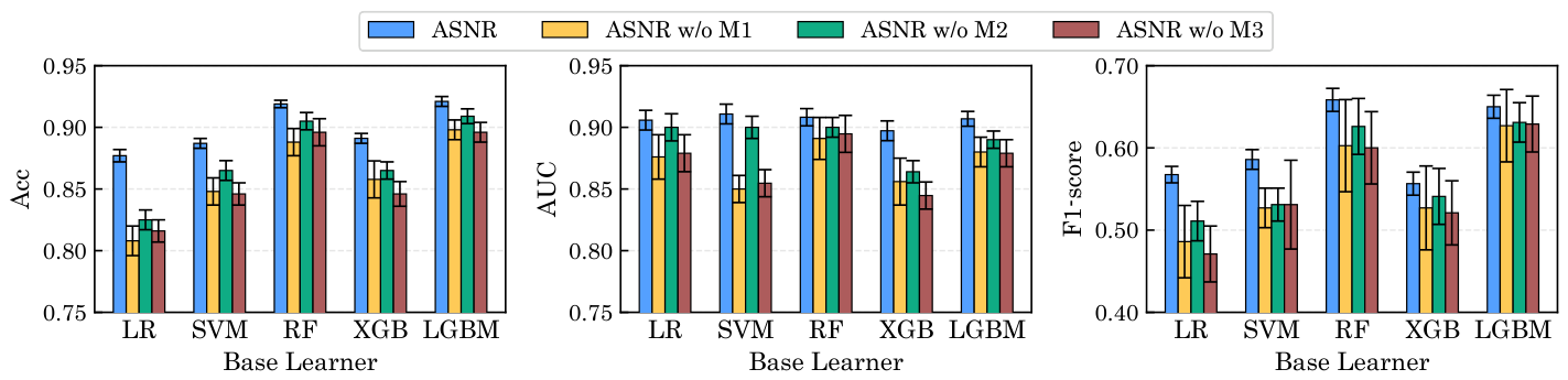
To verify the effectiveness of each ASNR component, we conduct ablation experiments with five base learners, namely LR, SVM, RF, XGB, and LGBM. The results are shown in Figure 6. Specifically, w/o M1 removes feature weighting by setting all feature weights to 1, w/o M2 replaces spherical neighborhood-based noise filtering and key seed identification with the conventional KNN strategy ($k=5$), and w/o M3 removes sampling weights and randomly samples from all candidate points.

As shown in Figure 6, the complete ASNR achieves the best Acc, AUC, and F1-score across all base learners, while each ablated variant shows performance degradation. The decline of w/o M1 indicates that indicator-level weights help ASNR construct more discriminative neighborhoods and guide interpolation along more informative feature dimensions. The decline of w/o M3 further shows that sample-level weights help allocate synthetic samples to more informative boundary regions. In addition, the results of w/o M2 suggest that spherical neighborhood-based sample categorization is more effective than conventional KNN for selecting representative boundary seeds. These findings confirm the effectiveness of the proposed ASNR architecture.

5.5.3. Effectiveness of the crER-Fusion

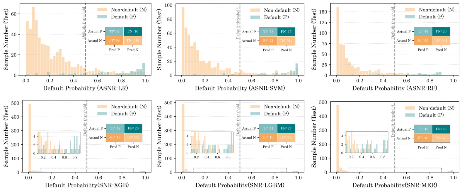
Figure 7 presents the default probability histograms and confusion matrices of the crER-fusion model and its five base classifiers (LR, SVM, RF, XGB, and LGBM) on the test set. Among the base learners, the linear models show a right-skewed distribution for non-default samples, with a clear peak and a long right tail. The extension of this tail beyond the classification threshold leads to high false positives (FPs). RF partially compresses this tail, but at the cost of fewer true positives (TPs) and lower recall. In contrast, the Gradient-Boosting learners (XGBoost and LightGBM) compress the predicted default probabilities of about 77% of non-default samples to near zero, i.e., $450/(19+567)$, thereby substantially reducing FP (XGB: FP = 19; LGBM: FP = 16). By synthesizing these outputs, crER fusion inherits the strong distributional separability of tree-based learners while improving the identification of high-confidence default samples. Specifically, crER fusion matches the minimum FP count of LightGBM (FP = 16) and further increases default detection (TP = 43). This result can be attributed to the evidential fusion mechanism of crER, which improves the precision–recall trade-off by discounting unreliable evidence from specific base learners and emphasizing high-confidence evidence.

5.6. Temporal Dynamics of Risk Indicators: A SHAP-Based Interpretation

5.6.1. Temporal Shifts in Indicator Category Importance

To examine how predictive information changes across time windows, the selected indicators are grouped into financial, non-financial, and macroeconomic categories. Their relative importance is measured by the cumulative absolute SHAP values within each category.

Table 15. SHAP value proportions of three indicator types across time windows.

Dataset	Financial Indicators (SHAP)	Non-Financial Indicators (SHAP)	Macroeconomic Indicators (SHAP)
t-0	30 (0.705)	6 (0.083)	16 (0.212)
t-1	29 (0.685)	4 (0.078)	15 (0.238)
t-2	23 (0.608)	5 (0.131)	19 (0.261)
t-3	20 (0.605)	4 (0.089)	15 (0.304)
t-4	18 (0.581)	3 (0.066)	20 (0.353)
t-5	14 (0.535)	2 (0.075)	11 (0.391)

reports the number of selected indicators and the corresponding SHAP share for each category. Table 15 shows that financial indicators remain the dominant predictors across all windows, although their contribution decreases from 0.7050 in t-0 to 0.5346 in t-5. By contrast, the contribution of macroeconomic indicators increases steadily from 0.2120 to 0.3909, indicating that external conditions become more informative as the prediction horizon extends. Non-financial indicators contribute less overall, but their share peaks at 0.1307 in t-2, suggesting that shareholding structure and corporate governance provide limited but useful incremental information in the medium term.

Economically, financial indicators capture solvency, profitability, operating efficiency, and growth capacity, making them the core signals of default risk. As the horizon lengthens, current financial information becomes less explanatory, while macroeconomic conditions exert a stronger influence through financing constraints, market demand, and cash-flow stability. These patterns indicate that default risk drivers shift over time: financial indicators dominate short-term prediction, non-financial indicators add modest medium-term information, and macroeconomic indicators become increasingly important for long-term prediction.

5.6.2. Time-Varying Influence of Key Predictors

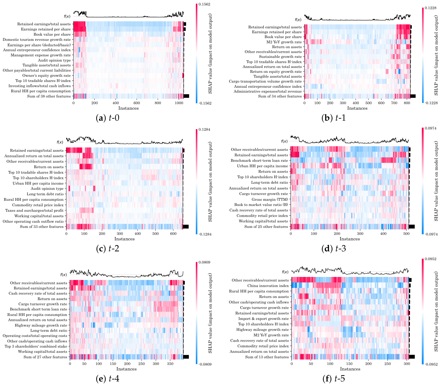
Figure 8 ranks the top predictors by SHAP value across six successive time windows. The results reveal three dynamic patterns of default risk formation.

(1) Financial indicators remain central, but their roles change over time. From t-0 to t-2, “Retained earnings/total assets” ranks first, indicating that internal capital accumulation is a key signal of short- and medium-term solvency. Weak retained earnings imply limited self-financing capacity and thinner loss-absorbing buffers, making firms more exposed to default pressure. From t-3 onward, “Other receivables/current assets” becomes the leading predictor, suggesting that earlier default signals are increasingly reflected in asset quality and liquidity occupation. A high share of other receivables may reflect delayed cash recovery, inefficient capital use, related-party occupation, or hidden agency problems, which can erode liquidity and evolve into future credit risk. “Annualized return on assets” remains important from t-1 to t-5, showing that profitability matters throughout the prediction process, especially when it supports stable cash-flow generation.

(2) Macroeconomic indicators show horizon-specific effects. In the short term, the “Annual entrepreneur confidence index” captures business sentiment and the external operating environment, which are closely linked to firms near default. At the medium horizon, “Urban HH per capita income” becomes more prominent, suggesting that demand conditions begin to affect repayment capacity. At longer horizons, “Rural HH per capita consumption”, “Cargo turnover growth rate”, and “Import & export growth rate” gain importance, reflecting consumption demand, logistics activity, and trade conditions. The high ranking of the “China innovation index” at t-5 further indicates that innovation-related conditions may shape firms’ long-run resilience to financial distress.

(3) Governance variables play a stage-specific role. Ownership concentration indicators, such as “Top 10 tradable shares H-index” and “Top 10 shareholders H-index”, become more important around t-2 and t-3. This suggests that ownership structure provides incremental information for medium-term default prediction. Concentrated ownership may improve monitoring, but excessive control concentration can intensify agency conflicts, facilitate resource occupation by controlling shareholders, and weaken liquidity. Thus, governance risk may gradually translate into future default risk.

6. Discussion

Our findings support two widely recognized points. First, oversampling is effective for mitigating class imbalance in credit risk prediction. Second, financial information remains the main driver of corporate default, while non-financial and macroeconomic variables also provide useful signals. Building on these points, this study extends existing research through method integration and multi-window prediction.

Compared with SMOTE, Borderline-SMOTE, and KMeans-SMOTE, ASNR retains the basic interpolation logic but further differentiates both indicators and minority samples. By assigning weights at the feature and sample levels, ASNR guides synthetic sample generation toward informative boundary regions and improves default identification under class imbalance, as shown in Table 7 and Table 8. Compared with deep generative methods such as CTGAN, ASNR also offers a more traceable sampling process, which is important for interpretable financial risk management. In addition, ASNR-crER does not treat resampling as an isolated preprocessing step. Instead, ASNR is embedded into ensemble training, allowing sample generation and classifier learning to be jointly adjusted, while crER fuses base-learner probabilities by considering class-specific reliability. The results in Table 9 and Table 10 suggest that reliability-aware evidence fusion combined with adaptive resampling is more effective than traditional ensemble strategies such as Boosting, Bagging, and Stacking for imbalanced default prediction. The six-window comparison in Section 5.3 further highlights the value of dynamic prediction. Although model performance changes as the prediction horizon lengthens, ASNR-crER maintains its advantage across different windows. This suggests that default risk evolves over time and cannot be fully captured by a single-window model. The SHAP analysis in Section 5.5 provides further evidence from a global interpretability perspective, showing that different risk signals play different roles at different stages of default evolution. Although inter-firm contagion and network effects are not explicitly modeled in this study, the multi-window outputs and indicator-level interpretations help explain how financial vulnerability changes over time. They also provide a basis for future research incorporating firm networks, industry links, or supply-chain relationships.

7. Conclusions and Future Work

This paper proposes ASNR-crER, a resampling ensemble framework for multi-window corporate default prediction under severe class imbalance. Using Chinese listed small enterprises as the research object, this study addresses three connected issues: insufficient learning from minority default samples, decision conflicts among heterogeneous base learners, and limited interpretation of time-varying default risk drivers. The main findings are summarized as follows. (1) ASNR outperforms conventional resampling methods, including SMOTE, Borderline-SMOTE, KMeans-SMOTE, and several generative sampling methods. Across the six prediction windows, ASNR improves accuracy, AUC, and F1-score, with especially notable gains in F1. This indicates that default samples should not be expanded mechanically; instead, synthetic samples should be generated around informative boundary firms while reducing the influence of outliers and low-value samples. (2) The comparison with imbalanced prediction benchmarks shows that ASNR-crER achieves better overall performance in small-enterprise default prediction. The ablation results further indicate that, under class imbalance, combining data-level imbalance correction with model-level evidential fusion helps improve the classification accuracy of both default and non-default firms and provides useful support for corporate default risk identification. (3) As the prediction horizon lengthens, model performance generally declines, reflecting the gradual weakening of firm-level default signals. Nevertheless, ASNR-crER maintains relatively stable performance across different windows. SHAP results further show that default risk drivers vary across horizons: financial indicators dominate short-term prediction, while macroeconomic and non-financial indicators provide complementary signals in medium- and long-term windows. Therefore, corporate default prediction should be treated within a dynamic multi-window framework, which better captures default risk evolution and supports both short-term identification and long-term early warning.

Collectively, the contribution of this study lies in integrating feature- and sample-aware resampling, class-specific reliability-based evidence fusion, and multi-window interpretability into a unified default prediction framework. This integration provides a more targeted solution for imbalanced small-enterprise default prediction and offers useful methodological support for dynamic financial risk management. However, this study still has several limitations. First, robustness is evaluated mainly from the perspective of empirical stability across prediction windows, repeated runs, and extended samples. Adversarial-noise and perturbation-based robustness tests are not included in the current experimental design. Future research may further examine the sensitivity of the proposed model to feature perturbations and noisy observations. Second, this study defines default using ST or *ST status and treats the task as binary classification. This setting is effective for identifying default-like firms, but cannot distinguish different stages or types of financial distress. Future research will construct multi-class or multi-label risk states to provide more refined early-warning signals. Third, the current SHAP analysis mainly explains global feature importance and time-varying contributions. Future work will extend the interpretability module from firm-level, causal, and counterfactual perspectives, so that the model can better explain why a specific enterprise is at risk and how changes in key indicators may affect its default probability.

References

1. Barth, M.E.; Ormazabal, G.; Taylor, D.J. Asset securitizations and credit risk. Account. Rev. 2012, 87, 423–448. [Google Scholar]
2. Chen, N.; Ribeiro, B.; Chen, A. Financial credit risk assessment: A recent review. Artif. Intell. Rev. 2016, 45, 1–23. [Google Scholar]
3. Chen, S.; Wang, J.Q.; Zhang, H.Y. A hybrid PSO-SVM model based on clustering algorithm for short-term atmospheric pollutant concentration forecasting. Technol. Forecast. Soc. Chang. 2019, 146, 41–54. [Google Scholar]
4. Altman, E.I. Financial ratios, discriminant analysis and the prediction of corporate bankruptcy. J. Financ. 1968, 23, 589–609. [Google Scholar] [CrossRef]
5. Desai, V.S.; Crook, J.N.; Overstreet, G.A., Jr. A comparison of neural networks and linear scoring models in the credit union environment. Eur. J. Oper. Res. 1996, 95, 24–37. [Google Scholar] [CrossRef]
6. Miguéis, V.L.; Benoit, D.F.; Van den Poel, D. Enhanced decision support in credit scoring using Bayesian binary quantile regression. J. Oper. Res. Soc. 2013, 64, 1374–1383. [Google Scholar] [CrossRef]
7. Moscatelli, M.; Parlapiano, F.; Narizzano, S.; Viggiano, G. Corporate default forecasting with machine learning. Expert Syst. Appl. 2020, 161, 113567. [Google Scholar] [CrossRef]
8. Tsai, C.F.; Sue, K.L.; Hu, Y.H.; Chiu, A. Combining feature selection, instance selection, and ensemble classification techniques for improved financial distress prediction. J. Bus. Res. 2021, 130, 200–209. [Google Scholar] [CrossRef]
9. Zhang, W.; Yang, D.; Zhang, S. A new hybrid ensemble model with voting-based outlier detection and balanced sampling for credit scoring. Expert Syst. Appl. 2021, 174, 114744. [Google Scholar] [CrossRef]
10. Chen, T.; Zhang, R.; Jian, H. An interpretable credit default risk prediction framework integrating causal feature selection and double machine learning. Systems 2026, 14, 327. [Google Scholar] [CrossRef]
11. Sun, J.; Shang, Z.; Li, H. Imbalance-oriented SVM methods for financial distress prediction: A comparative study among the new SB-SVM-ensemble method and traditional methods. J. Oper. Res. Soc. 2014, 65, 1905–1919. [Google Scholar]
12. Zhang, X.; Zhang, T.; Hou, L.; Liu, X.; Guo, Z.; Tian, Y.; Liu, Y. Data-driven loan default prediction: A machine learning approach for enhancing business process management. Systems 2025, 13, 581. [Google Scholar] [CrossRef]
13. Smiti, S.; Soui, M. Bankruptcy prediction using deep learning approach based on borderline SMOTE. Inf. Syst. Front. 2020, 22, 1067–1083. [Google Scholar] [CrossRef]
14. Jiang, C.; Zhou, Y.; Chen, B. Mining semantic features in patent text for financial distress prediction. Technol. Forecast. Soc. Chang. 2023, 190, 122450. [Google Scholar] [CrossRef]
15. Liu, W.; Suzuki, Y.; Du, S. Ensemble learning algorithms based on easyensemble sampling for financial distress prediction. Ann. Oper. Res. 2025, 346, 2141–2172. [Google Scholar] [CrossRef]
16. Duan, W.; Hu, N.; Xue, F. The information content of financial statement fraud risk: An ensemble learning approach. Decis. Support Syst. 2024, 182, 114231. [Google Scholar] [CrossRef]
17. Abedin, M.Z.; Chen, G.; Hajek, P.; Zhang, T. Combining weighted SMOTE with ensemble learning for the class-imbalanced prediction of small business credit risk. Complex Intell. Syst. 2023, 9, 3559–3579. [Google Scholar]
18. Chen, T.K.; Liao, H.H.; Chen, G.D.; Kang, W.H.; Lin, Y.C. Bankruptcy prediction using machine learning models with the text-based communicative value of annual reports. Expert Syst. Appl. 2023, 233, 120714. [Google Scholar] [CrossRef]
19. He, H.; Zhang, W.; Zhang, S. A novel ensemble method for credit scoring: Adaption of different imbalance ratios. Expert Syst. Appl. 2018, 98, 105–117. [Google Scholar] [CrossRef]
20. Zhang, T.; Zhu, W.; Wu, Y.; Wu, Z.; Zhang, C.; Hu, X. An explainable financial risk early warning model based on the DS-XGBoost model. Financ. Res. Lett. 2023, 56, 104045. [Google Scholar] [CrossRef]
21. Geng, X.; Wang, H.; Yan, L. Interpretable AI for financial risk perception: A machine learning approach to corporate crisis prediction. Financ. Res. Lett. 2025, 89, 109317. [Google Scholar]
22. Lei, X.; Lin, L.; Xiao, B.; Yu, H. Re-exploration of small and micro enterprises’ default characteristics based on machine learning models with SHAP. Chin. J. Manag. Sci. 2024, 32, 5. [Google Scholar]
23. Barboza, F.; Kimura, H.; Altman, E. Machine learning models and bankruptcy prediction. Expert Syst. Appl. 2017, 83, 405–417. [Google Scholar] [CrossRef]
24. Tang, X.; Li, S.; Tan, M.; Shi, W. Incorporating textual and management factors into financial distress prediction: A comparative study of machine learning methods. J. Forecast. 2020, 39, 769–787. [Google Scholar] [CrossRef]
25. Papouskova, M.; Hajek, P. Two-stage consumer credit risk modelling using heterogeneous ensemble learning. Decis. Support Syst. 2019, 118, 33–45. [Google Scholar] [CrossRef]
26. Zhang, Z.; Wu, C.; Qu, S.; Chen, X. An explainable artificial intelligence approach for financial distress prediction. Inf. Process. Manag. 2022, 59, 102988. [Google Scholar] [CrossRef]
27. Papík, M.; Papíková, L. Impacts of crisis on SME bankruptcy prediction models’ performance. Expert Syst. Appl. 2023, 214, 119072. [Google Scholar]
28. Gnip, P.; Kanász, R.; Zoričak, M.; Drotár, P. An experimental survey of imbalanced learning algorithms for bankruptcy prediction. Artif. Intell. Rev. 2025, 58, 104. [Google Scholar] [CrossRef]
29. Tang, J.; Li, Y.; Hou, Z.; Fu, S.; Tian, Y. Robust two-stage instance-level cost-sensitive learning method for class imbalance problem. Knowl.-Based Syst. 2024, 300, 112143. [Google Scholar]
30. Wang, S.; Chi, G. Cost-sensitive stacking ensemble learning for company financial distress prediction. Expert Syst. Appl. 2024, 255, 124525. [Google Scholar] [CrossRef]
31. Xia, Y.; Han, Z.; Li, Y.; He, L. Credit scoring model for fintech lending: An integration of large language models and FocalPoly loss. Int. J. Forecast. 2025, 41, 894–919. [Google Scholar]
32. Chen, Z.; Liu, Y.; Liu, X.; Dong, J. Forecasting Corporate Bankruptcy Through Class-Rebalanced Self-Training Semi-Constrained Matrix Factorization. J. Forecast. 2026, 45, 530–546. [Google Scholar]
33. Xia, M.; Wang, Z.; Lan, X.; Liu, W.; Wu, J. Confidence-driven under-sampling decision forest for imbalanced credit scoring. Eng. Appl. Artif. Intell. 2025, 147, 110278. [Google Scholar]
34. Zhou, Y.; Shen, L.; Ballester, L. A two-stage credit scoring model based on random forest: Evidence from Chinese small firms. Int. Rev. Financ. Anal. 2023, 89, 102755. [Google Scholar] [CrossRef]
35. Zhou, Y.; Lin, X.; Chi, G.; Jin, P.; Li, M. EWT-SMOTE to improve default prediction performance in imbalanced data: Analysis of Chinese data. J. Forecast. 2024, 43, 615–643. [Google Scholar]
36. Smiti, S.; Soui, M.; Ghedira, K. Tri-XGBoost model improved by BLSmote-ENN: An interpretable semi-supervised approach for addressing bankruptcy prediction. Knowl. Inf. Syst. 2024, 66, 3883–3920. [Google Scholar]
37. Chai, N.; Abedin, M.Z.; Yang, L.; Shi, B. Farmers’ credit risk evaluation with an explainable hybrid ensemble approach: A closer look in microfinance. Pac.-Basin Financ. J. 2025, 89, 102612. [Google Scholar]
38. Douzas, G.; Bacao, F.; Last, F. Improving imbalanced learning through a heuristic oversampling method based on k-means and SMOTE. Inf. Sci. 2018, 465, 1–20. [Google Scholar] [CrossRef]
39. Koziarski, M.; Krawczyk, B.; Woźniak, M. Radial-based oversampling for noisy imbalanced data classification. Neurocomputing 2019, 343, 19–33. [Google Scholar] [CrossRef]
40. Barua, S.; Islam, M.M.; Yao, X.; Murase, K. MWMOTE–Majority weighted minority oversampling technique for imbalanced data set learning. IEEE Trans. Knowl. Data Eng. 2014, 26, 405–425. [Google Scholar]
41. Li, M.; Zhou, H.; Liu, Q.; Gong, X.; Wang, G. WRND: A weighted oversampling framework with relative neighborhood density for imbalanced noisy classification. Expert Syst. Appl. 2024, 241, 122593. [Google Scholar]
42. Xue, W.; Duan, L.; Hong, X.; Zheng, X. Adaptive weighting and nearest neighbor-based area control for imbalanced data classification. Appl. Soft Comput. 2025, 177, 113171. [Google Scholar] [CrossRef]
43. Wang, S.; Bao, Y.; Yang, S. HS-SMOTE: Oversampling method for multiple dynamic interpolations based on regular hexagon scoring mechanism. Expert Syst. Appl. 2025, 265, 125855. [Google Scholar]
44. Gulrajani, I.; Ahmed, F.; Arjovsky, M.; Dumoulin, V.; Courville, A. Improved training of Wasserstein GANs. In Proceedings of the 31st Conference on Neural Information Processing Systems, Long Beach, CA, USA, 4–9 December 2017. [Google Scholar]
45. Habibi, O.; Chemmakha, M.; Lazaar, M. Imbalanced tabular data modelization using CTGAN and machine learning to improve IoT Botnet attacks detection. Eng. Appl. Artif. Intell. 2023, 118, 105669. [Google Scholar]
46. Kotelnikov, A.; Baranchuk, D.; Rubachev, I.; Babenko, A. TabDDPM: Modelling tabular data with diffusion models. In International Conference on Machine Learning; PMLR: Cambridge, MA, USA, 2023; pp. 17564–17579. [Google Scholar]
47. Hussain, A.B.; Jingchun, S.; Hussain, B.; Shaique, M.; Rehman, A.U.; Bhatti, M.K. Cross-Market Bankruptcy Prediction: An Interpretable Ensemble Learning Framework Using SHAP Analysis. Comput. Econ. 2026, 1–46. [Google Scholar] [CrossRef]
48. Lin, Y.C.; Padliansyah, R.; Lu, Y.H.; Liu, W.R. Bankruptcy prediction: Integration of convolutional neural networks and explainable artificial intelligence techniques. Int. J. Account. Inf. Syst. 2025, 56, 100744. [Google Scholar] [CrossRef]
49. Chawla, N.V.; Bowyer, K.W.; Hall, L.O.; Kegelmeyer, W.P. SMOTE: Synthetic minority over-sampling technique. J. Artif. Intell. Res. 2002, 16, 321–357. [Google Scholar] [CrossRef]
50. Antonio, B.O.; Juan, L.R.; Ana, I.D.; Fransisco, L.C. Examining user behavior with machine learning for effective mobile peer-to-peer payment adoption. Financ. Innov. 2024, 10, 94. [Google Scholar]
51. Li, C.; Lou, C.; Luo, D.; Xing, K. Chinese corporate distress prediction using LASSO: The role of earnings management. Int. Rev. Financ. Anal. 2021, 76, 101776. [Google Scholar] [CrossRef]
52. Zhou, H.; Du, J.; Zheng, X. Oversampling classification method based on neighborhood analysis on imbalanced data. Appl. Soft Comput. 2026, 190, 114565. [Google Scholar] [CrossRef]
53. Yang, J.-B.; Singh, M.G. An evidential reasoning approach for multiple-attribute decision-making with uncertainty. IEEE Trans. Syst. Man. Cybern. 1994, 24, 1–18. [Google Scholar]
54. Yang, J.-B.; Xu, D.-L. Evidential reasoning rule for evidence combination. Artif. Intell. 2013, 205, 1–29. [Google Scholar] [CrossRef]
55. Cui, S.; Gao, R.; Kuang, J.; Yang, L.; Qiu, H.; Wei, X. An interpretable imbalance ensemble classification method for readmission risk assessment incorporating multi-view perturbation and SHAP analysis. Decis. Support Syst. 2025, 190, 114404. [Google Scholar] [CrossRef]
56. Lundberg, S.M.; Lee, S.I. A unified approach to interpreting model predictions. In Advances in Neural Information Processing Systems 30; Curran Associates, Inc.: Red Hook, NY, USA, 2017. [Google Scholar]
57. Zhao, Q.; Xu, W.; Ji, Y. Predicting financial distress of Chinese listed companies using machine learning: To what extent does textual disclosure matter? Int. Rev. Financ. Anal. 2023, 89, 102770. [Google Scholar] [CrossRef]
58. Meng, Q.; Zheng, X.; Wang, S. Corporate governance and financial distress in China: A multi-dimensional nonlinear study based on machine learning. Pac.-Basin Financ. J. 2024, 88, 102549. [Google Scholar] [CrossRef]
59. Sun, W.; Chi, G.; Zhou, Y.; Dong, Y. Multi-window weighted random forests for listed companies default prediction: A dual-criterion temporal framework with hybrid feature selection. Ann. Oper. Res. 2026, 1–34. [Google Scholar] [CrossRef]
60. Sun, J.; Li, H.; Fujita, H.; Fu, B.; Ai, W. Class-imbalanced dynamic financial distress prediction based on AdaBoost-SVM ensemble combined with SMOTE and time weighting. Inf. Fusion 2020, 54, 128–144. [Google Scholar]
61. Zhao, F.; Li, G.; Lyu, Y.; Ma, H.; Zhu, X. A cost-sensitive ensemble deep forest approach for extremely imbalanced credit fraud detection. Quant. Financ. 2023, 23, 1397–1409. [Google Scholar] [CrossRef]
62. Xiao, J.; Zhong, Y.; Jia, Y.; Wang, Y.; Li, R.; Jiang, X.; Wang, S. A novel deep ensemble model for imbalanced credit scoring in internet finance. Int. J. Forecast. 2024, 40, 348–372. [Google Scholar]
63. Han, D.; Guo, W.; Chen, Y.; Wang, B.; Li, W. Personal credit default prediction fusion framework based on self-attention and cross-network algorithms. Eng. Appl. Artif. Intell. 2024, 133, 107977. [Google Scholar]
64. Shen, F.; Liu, Y.; Wang, R.; Zhou, W. A dynamic financial distress forecast model with multiple forecast results under unbalanced data environment. Knowl.-Based Syst. 2020, 192, 105365. [Google Scholar] [CrossRef]
Figure 1. The proposed ASNR-crER model.
Systems 14 00776 g001
Figure 2. Workflow of the crER fusion procedure.
Systems 14 00776 g002
Figure 3. Sample distribution of Chinese listed small enterprises. (a) Industry distribution of the sample; (b) Annual distribution of total, default, and non-default firm-year observations from 2000 to 2023.
Systems 14 00776 g003
Figure 4. Performance comparison across time windows.
Systems 14 00776 g004
Figure 5. Extended sample robustness test across prediction windows.
Systems 14 00776 g005
Figure 6. Ablation results of key ASNR modules (Acc, AUC, and F1 across five base learners).
Systems 14 00776 g006
Figure 7. Comparative analysis of probability distributions and confusion matrices.
Systems 14 00776 g007
Figure 8. SHAP contribution heatmaps for the top 15 predictors across six prediction windows. Negative SHAP values are shown in blue and indicate a negative contribution to the predicted default probability, while positive SHAP values are shown in red and indicate a positive contribution. The x-axis represents firms in the test set, and the f ( x ) curve shows how the predicted default probability changes with indicator values. By comparing the repeated occurrence and ranking changes in predictors across windows, the figure also provides evidence on the temporal stability and horizon-specific variation in default risk indicators.
Systems 14 00776 g008