Fiscal Decentralization and SDG6 Achievement: Evidence from AI-Based Estimation for OECD Countries

Abstract

Water and sanitation governance sits at the intersection of global development ambitions and highly localized service realities. While SDG6 sets universal targets for clean water and sanitation, the institutional and fiscal arrangements that translate those targets into actual service outcomes operate primarily at the subnational level. The discrepancy between globally defined objectives and locally executed delivery creates a structural research gap: how do the fiscal architectures of local governments influence progress towards SDG6? This study addresses this question for a panel of OECD countries by developing a deep learning-based estimation framework that combines bidirectional long short-term memory (BiLSTM) networks with Tianji’s horse racing optimization (THRO) algorithm. Three distinct operationalizations of fiscal decentralization are tested against SDG6 outcomes: subnational expenditure share (EFDM), subnational revenue share (RFDM), and a composite index balancing both dimensions (CFDM). Model adequacy is assessed using a layered diagnostic protocol involving regression fit, country-level residual patterns, error density profiles, Bland–Altman limits of agreement and inter-annual error trajectories. Among the three configurations, CFDM consistently records superior performance ($R^2=0.9216$; $RMSE = 1.4465$; $MAE = 1.0712$), while even the weakest specification clears $R^2=0.89$, attesting to the overall robustness of the proposed architecture. The margin by which CFDM outperforms its alternatives highlights a key finding: neither spending authority nor revenue capacity alone accurately reflects the fiscal reality of local water and sanitation governance; it is their combined effect that is important. The expenditure dimension is further proven to be the more influential of the two unidimensional proxies, consistent with the capital-intensive and maintenance-heavy nature of water infrastructure. On the other hand, coefficient findings show that fiscal decentralization is positively associated with SDG6 achievement for all models. Beyond its empirical contributions, the study introduces a methodological template for applying hybrid AI optimization to policy-relevant sustainability panels. It also connects two largely parallel bodies of scholarship, fiscal federalism and SDG research, that have rarely been examined together.

1. Introduction

Water is a crucial resource for public health, food security, ecosystem sustainability, and economic productivity [1,2,3,4]. Access to safe drinking water and sanitation is recognized as a fundamental human right [5], and it is also widely acknowledged as a key element shaping the social, economic and environmental dimensions of sustainable development [6,7]. The fundamental importance of water is universally acknowledged, yet access to water and sanitation remains one of the major development challenges at the global level today. Population growth, rapid urbanization and increasing impacts of climate change across the world are constantly increasing the demand for drinking water, sanitation and hygiene services, but improvements in service provision have not kept pace with the increasing demand [3]. Progress has been made in the global observation data but the current rate of progress is insufficient. As of 2024, only 74% of the world population has access to safe drinking water and 58% to safe sanitation services. Billions of people lack these basic services [8]. Access to water and sanitation services varies greatly between rural and urban areas, between countries at different stages of development, and between regions [9,10]. Limited water and sanitation access is not only an environmental challenge but a multidimensional global challenge for public health, food security and social welfare [6,7]. Water and sanitation governance has thus moved out of the purely technical service delivery domain and has become a structural issue at the centre of the global development agenda [11,12,13].

The shortcomings in access to clean water and sanitation were first incorporated into the global development agenda in 2000 under the millennium development goals (MDGs). Under the MDG framework, the international community committed to reducing by half the proportion of people lacking access to safe drinking water and basic sanitation by 2015. Although considerable progress was achieved during this period [14], the MDGs approached water and sanitation primarily through access-oriented and relatively narrow indicators, paying limited attention to service quality, continuity, wastewater management, water scarcity, and ecosystem dimensions [2]. These limitations highlighted the need for a more inclusive, holistic, and universal framework for water and sanitation in the post-2015 period. This need led to the adoption of the sustainable development goals (SDGs), also known as Agenda 2030, adopted by the United Nations, which present a more comprehensive development vision aimed at addressing the shortcomings of the MDGs [3]. The SDGs, consisting of seventeen integrated goals, provide a comprehensive development framework addressing a broad range of global challenges, including poverty, inequality, environmental sustainability, and governance. Among these goals, SDG6 plays a central role in sustainable development due to the critical importance of water and sanitation.

SDG6 aims to ensure availability and sustainable management of water and sanitation for all. This goal, which addresses the water cycle as a whole, encompasses multidimensional targets including safe drinking water, sanitation, and hygiene, as well as wastewater treatment, reduction in water pollution, water efficiency, combating water scarcity, protecting ecosystems, and integrated water resources management [2,14,15]. The multidimensional nature of SDG6 demonstrates that water and sanitation should not be viewed merely as a technical service area, but rather as a systemic policy domain that interacts directly with many SDGs, such as health, food security, poverty reduction, environmental sustainability, and economic productivity [3,6,7,16]. Thus, SDG6 is widely recognized as both a stand-alone goal and a cross-cutting objective that plays a critical enabling role in the achievement of other SDGs [17,18].

The actual provision of basic services covered by SDG6, such as drinking water supply, wastewater management, sanitation infrastructure, and water quality, is largely carried out by local governments; therefore, SDG6 performance is shaped at the city, regional, and community levels rather than at the national level [19,20,21]. Addressing the structural challenges associated with achieving SDG6 requires not only technical infrastructure investments but also strong local governance capacity, effective institutional coordination, sound investment planning, and efficient allocation of public expenditures. This is particularly relevant for infrastructure-intensive services that require continuous operation and maintenance financing. In these circumstances, the availability of adequate and sustainable local fiscal resources becomes a critical determinant of service quality and continuity, highlighting the importance of fiscal decentralization (FD) for effective local service delivery [22,23,24].

FD refers to the sharing of public functions and fiscal resources among different levels of government [25]. Traditional or first generation FD theory [25,26,27] outlines a normative framework for this sharing; it assigns the functions of macroeconomic stability and income redistribution to central governments, while assigning the function of providing goods and services within their own jurisdictions to local governments in order to improve efficiency in resource allocation. The traditional approach argues that the provision of public services by local governments can increase resource allocation efficiency and social welfare under conditions of heterogeneous local preferences [25,28,29]. In this regard, Tiebout (1956) argues that service efficiency can be increased through inter-local government competition and location choice based on individual preference matching [26]; Musgrave (1959) and Olson (1969) argue that the allocation of public functions and fiscal responsibilities among appropriate levels of government supports optimal resource allocation [27,30]. It is widely accepted that local governments can deliver public goods more efficiently, particularly under conditions of high local preference differences, limited externalities, and similar service costs [31]. While first generation approaches primarily emphasize local information advantages and allocative efficiency gains, second generation theories of FD focus on the role of incentives, accountability, institutional capacity, and intergovernmental relations in determining decentralization outcomes [32,33,34]. These approaches argue that FD does not necessarily lead to better public service performance. Rather, its success depends on fiscal discipline, local administrative capacity, accountability mechanisms, and effective coordination among levels of government. Variations in local fiscal capacity may also generate territorial disparities in service provision, while policy areas characterized by cross jurisdictional externalities may require stronger intergovernmental coordination [35].

Against this theoretical background, water and sanitation services provide a particularly relevant policy domain for evaluating both the opportunities and challenges associated with FD. The spatially differentiated demand structure of water and sanitation services, their high infrastructure dependency, and the continuous need for operational and maintenance financing make these services typical examples of local public services that can be evaluated within the framework of local allocative efficiency predicted by FD theory. Accordingly, FD emerges as a potentially decisive institutional mechanism for strengthening the accessibility, quality, and sustainability of water and sanitation services at the local level under SDG6. At the same time, the management of water resources often extends beyond administrative boundaries and may require substantial coordination among jurisdictions, while differences in local fiscal and administrative capacity may affect the quality and accessibility of service provision. The local service nature of water and sanitation also implies that the achievement of SDG6 may depend to a considerable extent on implementation outcomes at the local level [36]. Local governments represent the level of administration closest to citizens, which highlights their critical role in achieving SDG6 [37]. Achieving universal access to safe water and sanitation and ensuring the sustainable management of water resources therefore require strong alignment between global development objectives and local policy implementation. Sustainability in water and sanitation services therefore depends on the capacity of local governments to integrate social, economic, and environmental priorities into local policy frameworks and service delivery systems [36]. Recent studies highlight that the localization of SDGs, particularly in water and sanitation, plays a crucial role in translating global sustainability targets into effective local service outcomes [38]. Within this perspective, local governments are expected to play a leading role in advancing SDG6 by assessing local conditions, identifying needs and available resources, developing partnerships with stakeholders, and guiding appropriate policy actions and implementation strategies [39,40]. Integrating SDG6 objectives into local planning, budgeting, and service delivery processes therefore represents a key step in strengthening the accessibility, quality, and sustainability of water and sanitation services at the local level [37,38].

Although the determinants of sustainable development performance have been widely discussed in the literature, empirical studies that directly examine the role of FD on SDG6 remain relatively scarce. While the SDGs literature largely focuses on dimensions such as governance quality, institutional capacity, technical infrastructure, and policy design, the FD literature has developed primarily around macro-level variables such as economic growth, income distribution, and public expenditure efficiency. The limited overlap between these two strands of literature has resulted in an incomplete understanding of how local fiscal structures influence SDGs, particularly with respect to the accessibility, quality, and sustainability of water and sanitation services. Given the inherently local service character of SDG6, this gap highlights the need for a systematic analysis of how local fiscal capacity influences SDG6 performance. Beyond addressing this empirical gap, the study also offers a conceptual contribution by positioning SDG6 performance not only as an infrastructural and environmental outcome, but also as a governance outcome shaped by fiscal institutions and intergovernmental arrangements. While water and sanitation outcomes are commonly examined through technical, environmental, and policy-related determinants, this perspective highlights local fiscal structures as an institutional mechanism influencing service delivery performance. In doing so, the study brings together the FD and sustainable development studies within a common governance framework and contributes to a more comprehensive understanding of the institutional foundations of SDG6 performance.

To address this gap, this study empirically examines the relationship between FD and SDG6 performance in a sample of organization for economic co-operation and development (OECD) countries. Although access to clean water and sanitation services is often associated with low- and middle-income countries, it continues to persist as an area of inequality even in high income countries, particularly for rural, remote, and indigenous communities [9,21]. In this respect, in OECD countries, although past investments have significantly improved access levels, aging infrastructure, more stringent environmental regulations, and cost pressures associated with climate change have generated new financial and governance challenges in the water sector [41,42,43]. On the other hand, OECD countries provide a reliable setting for cross-country comparative analysis through standardized and comparable data structures related to SDG6; in this respect, the observed heterogeneity in water and sanitation outcomes, despite high income levels and institutional capacity, further allows for the examination of performance differentials through financial and governance dimensions [13,41]. For these reasons, the OECD sample offers a suitable empirical context for analyzing the relationship between FD and water and sanitation performance, as well as for testing related policy implications. The study contributes to literature in three complementary ways. First, by empirically testing the link between FD and SDG6, a relationship that has received limited attention in the sustainable development literature, it provides new evidence on the fiscal dimension of sustainable development performance. Second, it integrates the perspective of sustainable development goals into the FD literature, thereby offering a novel conceptual framework that examines the role of local fiscal capacity in the SDG6 achievement. Finally, the study extends traditional econometric approaches by incorporating artificial intelligence-based analytical techniques into the empirical analysis, thereby proposing an innovative methodological approach to examining the determinants of sustainable development performance. In this respect, the study aims to establish an analytical bridge between FD and sustainable development literature.

The remainder of this paper is organized as follows. Section 2 provides a comprehensive review of the existing literature examining the key determinants of SDG performance in general and SDG6 in particular. Section 3 presents the proposed analytical framework in detail, covering the dataset and variable definitions, the bidirectional long short-term memory (BiLSTM) architecture and its bidirectional extension, the Tianji’s horse racing optimization (THRO)-based hyperparameter optimization procedure, and the performance metrics employed for model evaluation. Section 4 reports empirical results and offers an in-depth discussion, including the predictive accuracy of the three FD models, the revenue-based FD model (RFDM), the expenditure-based FD model (EFDM), and the composite FD model (CFDM), and the relative importance of each determinant in shaping SDG6 outcomes across OECD countries. Section 5 concludes the paper by summarizing the principal findings, articulating their policy implications, and outlining directions for future research.

2. Literature Review

Economic, social, institutional, structural, and demographic factors play a decisive role in the achievement of the SDGs. Economic growth [44], inflation [45], globalization [46], public revenues [47], public expenditures [48], public budget balance [39], public investments [23], and the informal economy [49] are among the economic factors shaping the success of the SDGs. These factors influence SDGs achievement through macroeconomic stability, resource generation, and resource allocation. In terms of social impacts, unemployment [23] is also viewed as a factor limiting SDGs achievement by causing income loss, increased poverty, and social exclusion through the labor market. In addition to economic and social factors, the literature considers institutions to be a highly significant factor in SDGs achievement. Good governance [50], public sector transparency [51], and democratic institutional structures [46] are among the institutional factors that determine the effectiveness of public resource allocation and policy implementation related to the SDGs. On the other hand, technological development [52], digitalization [53], innovation performance [54], and artificial intelligence [52] are viewed as structural factors playing a critical role in the achievement of the SDGs. These elements enhance efficiency in public service delivery, facilitate data-driven policymaking, and enable the monitoring of SDGs progress. Another group of factors shaping SDGs achievement are demographic factors, which include socio-economic and cultural structures [55] and educational level [56] are argued to be decisive in terms of the social acceptance, feasibility, and long-term effectiveness of policies aimed at the SDGs.

Literature also demonstrates the existence of studies regarding the specific forms of the SDGs. Among these, SDG6 is gaining increasing attention as a goal that impacts other SDGs as well; however, there remains a limited number of empirical studies in this area [21]. The SDG6 literature addresses numerous factors that shape performance success. Financial capacity [15] is the first key factor in this regard. The water and sanitation sector is capital-intensive, requiring infrastructure investments [57] and resulting in ongoing operational and maintenance costs [58]. These conditions necessitate financial adequacy for the sector. Financial sustainability, in turn, is closely linked to the pricing policies of water and sanitation services. In this regard, sustainable pricing policies that cover full costs are crucial for achieving sustainable SDG6 success [43,59]. In addition, it is argued that privatization [60,61] and public–private partnership [62] models could also be effective as alternatives to public financing in achieving SDG6. On the other hand, the literature emphasizes the importance of institutional coordination [63], political will [64], and multi-level governance arrangements for SDG6 achievement [65,66,67]. Governance is a decisive factor regarding policy coherence, resource allocation, and effective implementation in water and sanitation services [68]. OECD (2011) defines water governance as the totality of political, social, economic, and administrative systems available to develop and manage water resources and provide water services at various levels of society [69]. Governance improves environmental performance and enhances the achievement of SDG6 by shaping integrated water resources management practices [15,70,71,72]. Participation [73] and monitoring [74] are key governance indicators in achieving this success. Another determining factor for SDG6 achievement is technology. Technological capacity, digital monitoring systems, and data-driven policy tools influence SDG6 performance by enhancing the efficiency and effectiveness of service delivery [20,74,75]. In addition to financial, institutional, and technological factors, economic development [4,76], globalization [77], strict environmental regulations [13], risks stemming from climate change [10], population and urbanization [76,77,78,79] are also among the factors influencing the achievement of SDG6.

Local dynamics also play a role in the achievement of SDG6. Services related to SDG6 are primarily provided by local governments [19,21,60]. This makes SDG6, which has a global nature, a goal that must be considered by local governance actors and institutions, thereby bringing it to the forefront of local policies [80]. In essence, it can be stated that local governments bear a vital responsibility in achieving global-level targets. In addition to spatial heterogeneity and local development dynamics [81], the administrative and financial capacity of local governments is also a determining factor for the achievement of SDG6 [16,36,39]. From this perspective, FD should be evaluated as a potential institutional and financial mechanism that could influence the achievement of SDG6. FD plays a decisive role in the provision and financing of SDG6-related services through its expenditure and revenue dimensions [39]. Despite its significance, research on FD and SDG6 in the literature is quite limited and indirect.

Taiwo (2024) investigated the impact of FD on the MDGs using pooled ordinary least squares (OLS), fixed-effects, and random-effects estimation methods on panel data covering 68 countries and the period 1991–2014 [82]. The findings reveal that both revenue and expenditure decentralization have a positive effect on access to water and sanitation, and this effect is more prominent in rural areas. Although this study does not directly address SDG6, it is significant in terms of its contribution to the development of the literature. In another study, Martínez-Córdoba et al. (2020) used data from 356 local governments in Spain with populations ranging from 1000 to 50,000 for the 2014 and 2018 period to investigate the factors influencing SDG6 achievement using regression analysis [60]. The findings revealed that taxes related to water and sanitation, as well as local government revenues, have a positive impact on SDG6 achievement. Accordingly, while these indicators do not fully address FD, their positive effect on SDG6 is considered noteworthy. In another study conducted using the Spanish sample, Benito et al. (2025) examined the factors influencing 89 municipalities’ compliance with the SDGs for the year 2018 using OLS and two-stage least squares (2SLS) methods [83]. The findings indicate that compliance with the SDGs decreases in municipalities characterized by high unemployment and low tax revenue collection, while it increases in municipalities with high voter turnout. Similarly, this study also reflects the positive contribution of FD to the SDGs. In another study focusing on a different aspect of the relationship, Benito et al. (2023) examined the effect of compliance with the SDGs on the financial indicators of local governments across 96 municipalities in Spain using the 2SLS method [39]. The findings revealed that municipalities demonstrating greater compliance with the SDGs experienced a deterioration in budget balance and a weakening of fiscal capacity. Finally, Gariba et al. (2024) examined the impact of FD on the SDGs using an OECD sample [24]. Findings obtained using a structural equation modeling approach based on data from the 2016 and 2022 period revealed that FD has a negative effect on the economic dimension of the SDGs and a positive effect on their social and environmental dimensions. Based on these findings, it can be stated that FD has a positive effect on SDG6, which belongs to the environmental dimension.

While these studies offer valuable information regarding the nexus of FD and sustainable development outcomes, there are several gaps. First, empirical evidence specifically targeting the FD-SDG6 nexus is still limited. Second, the existing studies generally focus on the expenditure or revenue-based indicators separately, and evidence on the relative performance of alternative FD measures is scarce. Third, previous studies have mainly used conventional econometric approaches and provided scant evidence on the relative importance of fiscal, institutional and socio-economic determinants of SDG6 performance. Therefore, this study contributes to the existing literature by evaluating composite, expenditure and revenue-based FD measures in an AI-supported analytical framework and by providing a more comprehensive evaluation of factors associated with SDG6 performance.

3. Materials and Methods

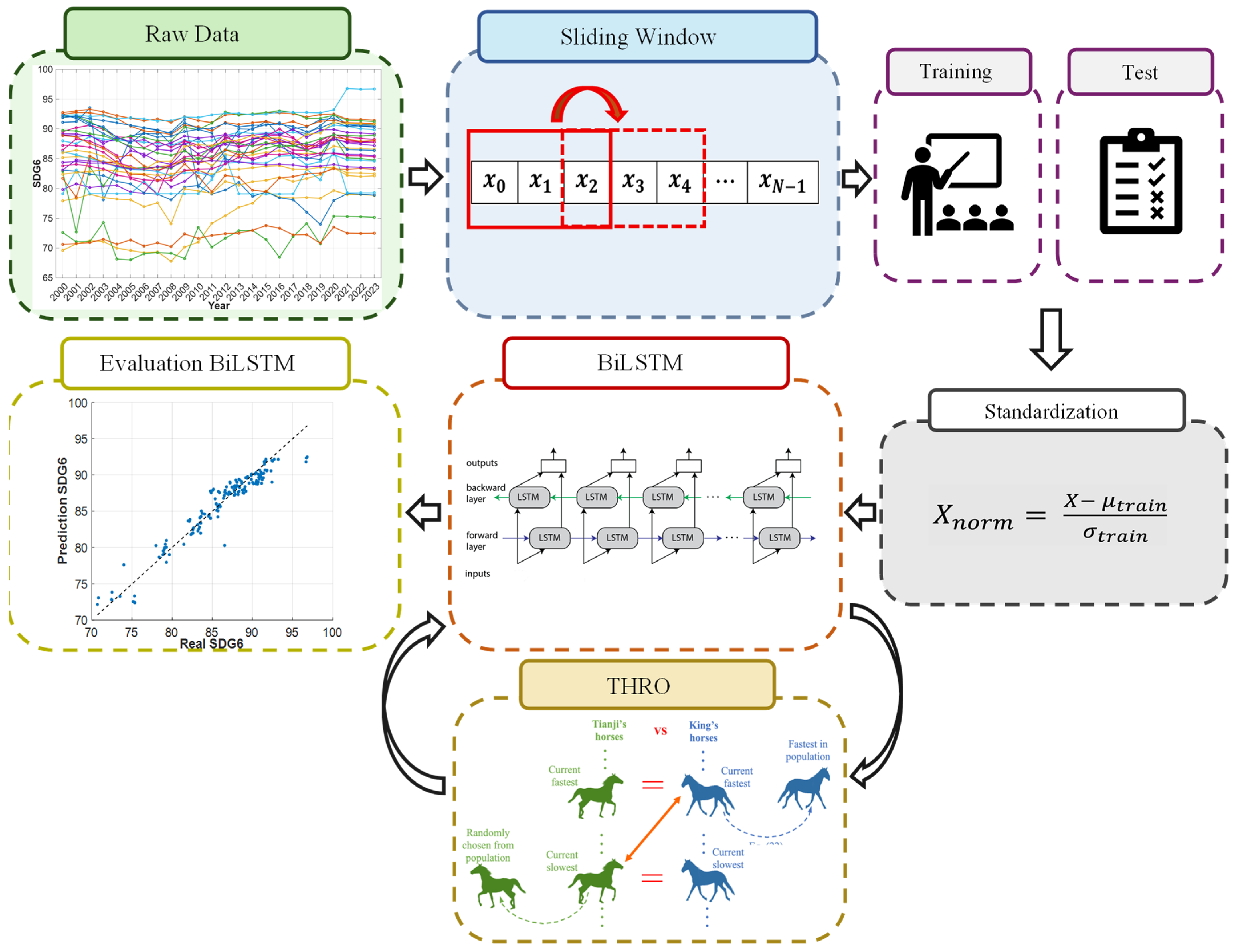
The primary objective of this research is to explore how FD influences water and sanitation services through an analytical framework grounded in artificial intelligence. For this purpose, a data-driven modeling strategy is constructed, combining advanced deep learning method with metaheuristic optimization technique to capture the intricate and evolving relationships between fiscal variables and sustainable development outcomes. The proposed framework unfolds across several consecutive stages: data preprocessing, temporal feature construction, model development, hyperparameter tuning, and performance assessment. In the initial phase, the raw data is restructured into a format suitable for supervised learning by applying a sliding window technique, which effectively represents temporal dependencies. Next, BiLSTM architecture is used to extract sequential patterns moving in both directions embedded in the dataset. The predictive performance is then further strengthened by optimizing the model’s hyperparameters using Tianji’s Horse Racing Optimization (THRO) algorithm, which is integrated with a deterministic quick evaluation strategy. Finally, the model is rigorously tested on previously unseen data to confirm its robustness and ability to generalize across different conditions. Together, these components form a comprehensive analytical framework for examining the impact of FD on the achievement of SDG6 objectives among OECD member states. Figure 1 presents the complete architecture and operational workflow of the proposed model.

The modeling procedure consists of six sequential stages:

In the first stage, the raw dataset comprises annual socio-economic and institutional indicators1 for 2000–2023 period of 32 OECD member countries2, organized as multivariate time series. Each variable is structured on a yearly basis across all countries, enabling the investigation of whether the decentralization of expenditure and revenue authority to local governments leads to improvements in SDG6 performance.

In the second stage, country-level temporal data are restructured into supervised learning sequences through a sliding window procedure. Rather than inputting the complete time series directly into the model, a forward-moving window mechanism segments the data into overlapping subsets, generating multiple training samples per country while preserving the original chronological order. This segmentation strategy allows the model to recognize time-dependent patterns and sequential structures more effectively. For the purposes of this study, a window size of five was adopted.

In the third stage, the transformed dataset is partitioned into training and testing subsets following a time-based splitting criterion, which prevents any forward-looking information from contaminating the learning process. Observations recorded up to and including 2018 constitute the training set, whereas data from 2019 onward are withheld exclusively for evaluating out-of-sample predictive performance.

In the fourth stage, z-score standardization is applied to normalize all variables and eliminate discrepancies arising from differing measurement scales. The mean and standard deviation required for this transformation are derived solely from the training partition, after which identical statistics are applied to the test set, thereby ensuring that no information from future observations influences the normalization procedure.

In the fifth stage, the preprocessed sequences are fed into a BiLSTM network, an architecture well suited to learning temporal dependencies in both chronological directions simultaneously. To extract maximum predictive capability from this architecture, critical hyperparameters, namely the learning rate, hidden layer size, fully connected layer size, mini-batch size, and number of training epochs, are tuned through the THRO algorithm. The optimization procedure seeks the parameter configuration that minimizes prediction error while preserving the model’s ability to generalize to unseen observations.

In the concluding stage, the performance of the optimized model is thoroughly assessed by contrasting predicted outputs with observed SDG6 values across a suite of regression-based metrics, including $R^2$, $RMSE$, and $MAE$.

Complementary diagnostic analyses, comprising error distribution profiling, Bland–Altman agreement analysis, and temporal trend examination, are further conducted to validate the accuracy, internal consistency, and overall reliability of the proposed framework.

3.1. Dataset

The dataset employed in this study encompasses nine variables spanning the period under investigation, with full definitions, measurement approaches, and data sources summarized in

Table 1. Variables and data sources.

Variable	Definition	Measurement	Source
SDG6	Overall performance in clean water and sanitation	Composite index (0–100 scale; higher values indicate better performance)	UN Sustainable Development Solutions Network, Sustainable Development Report [84]
EFD	Expenditure-based fiscal decentralization	Subnational government expenditure as a share of GDP	OECD Fiscal Decentralization Database [85]
RFD	Revenue-based fiscal decentralization	Subnational government revenue as a share of GDP	OECD Fiscal Decentralization Database [85]
CFD	Composite fiscal decentralization index	$CFD={\displaystyle \frac{RFD}{1-EFD}}$	Author’s calculation based on OECD data
DUMMY	Government structure dummy	1 = federal, 0 = unitary	Author’s classification
GDP	Economic development	GDP per capita growth (annual %)	World Bank, World Development Indicators (WDI) [86]
GOV	Good governance	Average of six WGI (range: −2.5 to +2.5)	World Bank, Worldwide Governance Indicators (WGI) [87]
POP	Population size	Logarithm of total population	World Bank, WDI [86]
URB	Urbanization	Urban population as a share of total population	World Bank, WDI [86]

. In addition, the descriptive statistics of the variables are reported in Appendix A,

Table A1. The mean and standard deviation values of the variables.

Dummy	Country	Mean								Standard Deviation
		SDG6	EFD	RFD	CFD	GDP	POP	URB	GOV	SDG6	EFD	RFD	CFD	GDP	POP	URB	GOV
1	Australia	89.102	16.511	15.520	18.595	1.356	16.927	85.321	1.562	3.148	0.932	0.450	0.681	1.024	0.113	0.778	0.047
1	Austria	92.155	16.236	5.096	6.085	0.918	15.954	58.462	1.505	0.628	0.463	0.145	0.191	2.444	0.039	0.907	0.109
1	Belgium	74.317	21.305	9.883	12.638	1.087	16.204	97.699	1.280	4.293	2.646	1.661	2.532	2.127	0.060	0.326	0.092
1	Canada	87.490	27.609	22.442	31.017	0.919	17.361	80.852	1.584	0.973	1.388	0.515	1.113	2.315	0.077	0.700	0.065
1	Germany	83.198	17.968	16.134	19.676	1.090	18.225	76.717	1.460	2.657	0.899	0.836	1.158	2.405	0.012	0.836	0.064
1	Spain	84.095	19.397	10.269	12.762	0.970	17.630	78.803	0.912	1.597	1.808	1.109	1.530	3.631	0.051	1.660	0.160
1	Switzerland	82.224	18.726	16.087	19.801	0.994	15.890	73.667	1.730	1.680	0.926	0.528	0.851	1.890	0.070	0.224	0.042
1	United States	84.006	18.883	14.461	17.829	1.388	19.555	81.093	1.223	0.436	0.677	0.274	0.387	1.824	0.057	1.286	0.134
0	Costa Rica	71.657	1.365	1.368	1.387	2.714	15.339	72.430	0.601	2.494	0.248	0.182	0.187	2.528	0.083	7.391	0.064
0	Czechia	88.763	11.541	2.862	3.236	2.243	16.166	73.681	0.896	0.969	0.858	0.297	0.342	3.175	0.049	0.369	0.106
0	Denmark	88.197	32.414	15.438	22.844	1.078	15.538	86.893	1.769	1.143	1.814	1.649	2.341	2.225	0.034	1.099	0.078
0	Estonia	89.429	9.669	1.695	1.877	3.512	14.099	68.754	1.095	2.699	0.629	0.258	0.289	5.823	0.034	0.528	0.130
0	Finland	90.982	20.325	13.903	17.471	1.022	15.499	84.198	1.821	0.977	1.870	1.253	1.789	2.918	0.026	1.276	0.078
0	France	85.244	10.622	7.813	8.746	0.851	17.992	78.784	1.157	1.135	0.643	0.657	0.775	2.493	0.035	1.809	0.087
0	Greece	91.017	3.549	1.272	1.319	0.951	16.205	76.753	0.469	1.650	0.316	0.187	0.196	5.103	0.027	2.493	0.228
0	Hungary	92.835	9.318	4.671	5.190	2.785	16.105	68.994	0.685	1.575	2.907	1.112	1.375	3.264	0.016	2.661	0.217
0	Iceland	86.526	12.960	11.131	12.794	1.648	12.691	93.437	1.589	2.572	0.743	0.661	0.851	3.781	0.096	0.482	0.138
0	Ireland	79.557	5.576	1.800	1.942	3.758	15.329	61.820	1.463	2.083	4.164	0.826	0.962	6.501	0.094	1.561	0.076
0	Israel	71.860	5.048	3.339	3.517	1.766	15.876	91.968	0.612	1.040	0.288	0.133	0.136	2.652	0.135	0.500	0.075
0	Italy	80.006	14.413	6.897	8.060	0.405	17.893	69.056	0.599	2.276	0.737	0.450	0.557	3.409	0.019	1.506	0.107
0	Latvia	88.775	11.152	7.268	8.185	4.637	14.547	68.040	0.694	0.732	1.059	0.451	0.565	6.078	0.078	0.235	0.126
0	Lithuania	84.513	8.925	1.139	1.252	4.884	14.937	67.228	0.799	3.085	0.936	0.190	0.216	5.155	0.080	0.617	0.150
0	Luxembourg	80.335	4.641	2.596	2.724	0.776	13.182	88.754	1.696	2.170	0.392	0.363	0.387	2.869	0.138	2.405	0.046
0	Netherlands	86.752	13.879	4.144	4.818	1.143	16.633	86.945	1.655	2.054	0.938	0.497	0.616	2.338	0.040	5.085	0.076
0	New Zealand	88.128	4.374	4.107	4.297	1.421	15.311	86.375	1.755	2.235	0.447	0.403	0.439	1.623	0.093	0.257	0.060
0	Norway	86.501	15.061	8.583	10.122	0.746	15.419	79.895	1.709	1.729	1.642	0.757	1.059	1.576	0.069	2.473	0.050
0	Poland	82.895	13.392	6.455	7.455	3.894	17.450	60.793	0.666	0.539	0.634	0.531	0.630	2.247	0.009	0.644	0.132
0	Portugal	86.245	6.400	4.242	4.533	0.883	16.154	61.354	1.043	1.560	0.469	0.254	0.277	3.006	0.047	4.167	0.110
0	Slovak Rep.	87.720	6.413	1.982	2.116	3.345	15.503	54.676	0.675	1.278	1.511	0.344	0.354	3.469	0.005	0.895	0.078
0	Slovenia	84.171	8.855	2.298	2.522	2.152	14.535	53.086	0.928	1.167	0.554	0.152	0.169	3.575	0.025	1.663	0.048
0	Sweden	90.638	24.103	16.740	22.054	1.353	16.068	85.873	1.703	0.705	1.151	0.765	0.896	2.452	0.054	1.596	0.071
0	UK	87.389	10.879	3.393	3.809	1.030	17.964	81.657	1.408	2.365	1.111	0.174	0.232	3.357	0.048	1.885	0.099
	Mean_OECD32	85.210	13.172	7.657	9.396	1.803	16.068	76.064	1.211

, where the corresponding mean and standard deviation values are presented to provide an overview of their central tendency and dispersion prior to model estimation.

SDG6 data are obtained from the Sustainable Development Report published by the UN Sustainable Development Solutions Network, which provides cross-country comparable data on clean water and sanitation, including both the overall SDG6 index and its subcomponents. In this study, the analysis focuses on the aggregate SDG6 index, as it offers a comprehensive and policy-relevant measure of water and sanitation performance. Given the inherently multidimensional nature of SDG6, the composite index enables an integrated assessment of outcomes, while avoiding model fragmentation that would arise from estimating separate models for each sub-indicator. The index is expressed on a 0–100 scale, where higher scores indicate greater progress toward achieving SDG6 targets.

FD is measured using three alternative specifications that capture different dimensions of subnational fiscal structures in OECD countries. The analysis relies exclusively on GDP-based indicators obtained from the OECD FD Database. In this context, expenditure-based FD (EFD) is proxied by subnational government expenditure as a share of GDP, while revenue-based FD (RFD) is measured by subnational government revenue as a share of GDP. In addition, a composite FD index (CFD) is built to capture the joint influence of EFD and RFD. The index is calculated as $CFD = RFD/(1-EFD)$ following Martinez-Vazquez and Timofeev (2010) [88]. Since both RFD and EFD are expressed as a percentage of GDP, the CFD index is not limited to an upper value. The higher the value of the CFD, the better the fit between subnational revenue capacity and expenditure responsibilities. This means that local governments are more able to finance expenditure commitments from their own revenue base. Lower values of CFD, on the other hand, reflect a weaker link between the ability to generate revenues and the obligations to spend, and a stronger dependence on central fiscal arrangements. Thus, the CFD index is a composite measure of fiscal balance under decentralization arrangements and does not isolate revenue or spending decentralization. A set of control variables is included as input features in the BiLSTM model to account for socio-economics and structural and institutional factors affecting SDG6 performance. A dummy variable is used to distinguish between federal and unitary systems $(1=\mathrm{f}\mathrm{e}\mathrm{d}\mathrm{e}\mathrm{r}\mathrm{a}\mathrm{l}$; $0=\mathrm{u}\mathrm{n}\mathrm{i}\mathrm{t}\mathrm{a}\mathrm{r}\mathrm{y}$), capturing differences in institutional arrangements that may affect the allocation of responsibilities and the efficiency of water and sanitation service provision. Economic development is proxied by GDP per capita growth (annual %), obtained from the WDI, reflecting the role of economic capacity in supporting investments in water and sanitation infrastructure. Good governance is measured using a composite governance indicator constructed as the simple average of the six dimensions of the WGI estimates, ranging from −2.5 to +2.5, where higher values indicate better governance; this variable captures the effectiveness of public service delivery and regulatory capacity relevant for SDG6 outcomes. Population size is measured as the logarithm of total population accounting for scale effects and pressure on water resources and infrastructure. Urbanization is proxied by the share of the urban population in total population reflecting the role of settlement patterns in shaping access to water and sanitation services. Both population and urbanization data were obtained from the WDI database.

3.2. Bidirectional Long Short-Term Memory Networks

3.2.1. Recurrent Neural Networks and the Vanishing Gradient Problem

A recurrent neural network (RNN) processes a variable-length input sequence $({\mathit{x}}_1,{\mathit{x}}_2,\dots ,{\mathit{x}}_T)$, where ${\mathit{x}}_t\in {\mathbb{R}}^m$, by maintaining a hidden state ${\mathit{h}}_t=\varphi ({\mathit{W}}_h{\mathit{h}}_{t-1}+{\mathit{W}}_x{\mathit{x}}_t+\mathit{b})$, where $\varphi$ denotes a pointwise nonlinearity. Although standard RNNs are theoretically capable of modeling sequence dependencies, they often suffer from exponential decay or growth of gradients when trained via backpropagation through time (BPTT) [89], a phenomenon known as the vanishing/exploding gradient problem [90]. Bengio et al. showed that this instability is an intrinsic consequence of the spectral properties of the recurrence Jacobian: when the largest singular value of ${\mathit{W}}_h$ is less than unity, gradients vanish geometrically, preventing the network from learning dependencies spanning many time steps [90].

3.2.2. Long Short-Term Memory

Hochreiter and Schmidhuber (1997) proposed the Long Short-Term Memory (LSTM) unit to overcome this limitation [91]. The key innovation is a dedicated cell state ${\mathit{c}}_t\in {\mathbb{R}}^d$, a linear recurrence whose gradient pathway is protected by multiplicative gating. Let $[{\mathit{h}}_{t-1};{\mathit{x}}_t]\in {\mathbb{R}}^{d+m}$ denote the concatenation of the previous hidden state ${\mathit{h}}_{t-1}\in {\mathbb{R}}^d$ and the current input ${\mathit{x}}_t\in {\mathbb{R}}^m$. The LSTM transition at time step $t$ is defined by the following system of equations [91,92]:

$${\mathit{f}}_t=\sigma \left({\mathit{W}}_f\hspace{0.17em}[{\mathit{h}}_{t-1};{\mathit{x}}_t]+{\mathit{b}}_f\right)$$

(1)

$${\mathit{i}}_t=\sigma \left({\mathit{W}}_i\hspace{0.17em}[{\mathit{h}}_{t-1};{\mathit{x}}_t]+{\mathit{b}}_i\right)$$

(2)

$${\tilde{\mathit{c}}}_t=\mathrm{t}\mathrm{a}\mathrm{n}\mathrm{h}\left({\mathit{W}}_c\hspace{0.17em}[{\mathit{h}}_{t-1};{\mathit{x}}_t]+{\mathit{b}}_c\right)$$

(3)

$${\mathit{c}}_t={\mathit{f}}_t\odot {\mathit{c}}_{t-1}+{\mathit{i}}_t\odot {\tilde{\mathit{c}}}_t$$

(4)

$${\mathit{o}}_t=\sigma \left({\mathit{W}}_o\hspace{0.17em}[{\mathit{h}}_{t-1};{\mathit{x}}_t]+{\mathit{b}}_o\right)$$

(5)

$${\mathit{h}}_t={\mathit{o}}_t\odot \mathrm{t}\mathrm{a}\mathrm{n}\mathrm{h}({\mathit{c}}_t)$$

(6)

where $\sigma (z)=1/(1+e^{-z})\in (0,1)$ is the element-wise sigmoid function, $\odot$ is the Hadamard (element-wise) product, ${\mathit{W}}_{\{f,i,c,o\}}\in {\mathbb{R}}^{d\times (m+d)}$ are the gate weight matrices, and ${\mathit{b}}_{\{f,i,c,o\}}\in {\mathbb{R}}^d$ are the corresponding bias vectors.

Equation (1) defines the forget gate ${\mathit{f}}_t\in (0,1{)}^d$, which determines what fraction of the previous cell state ${\mathit{c}}_{t-1}$ is retained. The input gate ${\mathit{i}}_t\in (0,1{)}^d$ in Equation (2) controls how much of the candidate cell state ${\tilde{\mathit{c}}}_t\in (-1,1{)}^d$ (Equation (3)) is written into memory. The updated cell state in Equation (4) combines these two contributions via element-wise multiplication and addition, yielding a recurrence whose gradient along the ${\mathit{c}}_{t-1}$ path is scaled only by ${\mathit{f}}_t$, near unity under appropriate initialization, thus permitting gradients to propagate without vanishing over arbitrarily long horizons [92]. The output gate ${\mathit{o}}_t$ in Equation (5) filters which portion of the nonlinearly transformed cell state is exposed as the hidden state ${\mathit{h}}_t$ in Equation (6). Each directional LSTM layer contains ${\mathsf{\Theta }}_{\mathrm{L}\mathrm{S}\mathrm{T}\mathrm{M}}=4d(m+d)+4d$ learnable parameters.

3.2.3. Bidirectional Extension

A unidirectional LSTM, as defined by Equations (1)–(6), conditions the hidden state ${\mathit{h}}_t$ only on the left context $({\mathit{x}}_1,\dots ,{\mathit{x}}_t)$. For many sequence-labelling and classification tasks, the representation of position $t$ depends equally on right-context information $({\mathit{x}}_T,\dots ,{\mathit{x}}_{t+1})$. Schuster and Paliwal (1997) proposed the bidirectional extension by training two independent recurrent sublayers on the same sequence in opposite temporal directions and combining their outputs at every position [93]. Graves and Schmidhuber (2005) demonstrated that replacing plain RNN cells with LSTM units in both directions yields the BiLSTM, which achieves superior performance on phoneme classification compared to unidirectional LSTM counterpart [92].

Concretely, a forward LSTM sublayer, with parameter set ${\overrightarrow{\mathit{W}}}_{\{f,i,c,o\}},\hspace{0.17em}{\overrightarrow{\mathit{b}}}_{\{f,i,c,o\}}$, processes the sequence from $t=1$ to $t=T$:

$${\overrightarrow{\mathit{h}}}_t=\overrightarrow{\mathrm{L}\mathrm{S}\mathrm{T}\mathrm{M}}\left({\mathit{x}}_t,\hspace{0.17em}{\overrightarrow{\mathit{h}}}_{t-1}\right), {\overrightarrow{\mathit{h}}}_0=\mathbf{0}, t=1,\dots ,T$$

(7)

A backward LSTM sublayer, with an entirely independent parameter set ${\overleftarrow{\mathit{W}}}_{\{f,i,c,o\}},\hspace{0.17em}{\overleftarrow{\mathit{b}}}_{\{f,i,c,o\}}$, traverses the same sequence in reverse:

$${\overleftarrow{\mathit{h}}}_t=\overleftarrow{\mathrm{L}\mathrm{S}\mathrm{T}\mathrm{M}}\left({\mathit{x}}_t,\hspace{0.17em}{\overleftarrow{\mathit{h}}}_{t+1}\right), {\overleftarrow{\mathit{h}}}_{T+1}=\mathbf{0}, t=T,T-1,\dots ,1$$

(8)

The forward state ${\overrightarrow{\mathit{h}}}_t\in {\mathbb{R}}^d$ summarises the prefix $({\mathit{x}}_1,\dots ,{\mathit{x}}_t)$, and the backward state ${\overleftarrow{\mathit{h}}}_t\in {\mathbb{R}}^d$ summarises the suffix $({\mathit{x}}_T,\dots ,{\mathit{x}}_t)$. These two complementary representations are fused by concatenation:

$${\mathit{h}}_t=\left[{\overrightarrow{\mathit{h}}}_t\hspace{0.33em};\hspace{0.33em}{\overleftarrow{\mathit{h}}}_t\right]\in {\mathbb{R}}^{2d}, t=1,\dots ,T$$

(9)

where $[\hspace{0.17em}\cdot \hspace{0.17em};\hspace{0.17em}\cdot \hspace{0.17em}]$ denotes vertical vector concatenation. The resulting ${\mathit{h}}_t$ conditions on both the past and the future contexts of ${\mathit{x}}_t$ simultaneously [93]. The total parameter count of a single BiLSTM layer is therefore ${\mathsf{\Theta }}_{\mathrm{B}\mathrm{i}\mathrm{L}\mathrm{S}\mathrm{T}\mathrm{M}}=2\times \left[4d(m+d)+4d\right]$.

3.2.4. Stacked BiLSTM and Regularization

Hierarchical temporal features can be learned by stacking $L$ BiLSTM layers, where the concatenated output of layer $\mathcal{l}$ serves as the input to layer $\mathcal{l}+1$:

$${\mathit{h}}_t^{(\mathcal{l})}=\left[{\overrightarrow{\mathit{h}}}_t^{(\mathcal{l})};\hspace{0.17em}{\overleftarrow{\mathit{h}}}_t^{(\mathcal{l})}\right], {\mathit{x}}_t^{(\mathcal{l}+1)}={\mathit{h}}_t^{(\mathcal{l})}, \mathcal{l}=1,\dots ,L$$

(10)

Regularization is achieved via variational dropout [94,95], in which a binary mask ${\mathit{ϵ}}^{(\mathcal{l})}\sim \mathrm{B}\mathrm{e}\mathrm{r}\mathrm{n}\mathrm{o}\mathrm{u}\mathrm{l}\mathrm{l}\mathrm{i}(1-p{)}^d$ is sampled once per sequence and applied uniformly across all $T$ time steps within layer $\mathcal{l}$:

$${\tilde{\mathit{h}}}_t^{(\mathcal{l})}={\mathit{h}}_t^{(\mathcal{l})}\odot {\displaystyle \frac{{\mathit{ϵ}}^{(\mathcal{l})}}{1-p}}, p\in [0,1).$$

(11)

Gal and Ghahramani (2016) provided a Bayesian justification for this approach, demonstrating that it corresponds to approximate variational inference in a deep Gaussian process [95]. They also showed that it achieves consistent improvements over naive per-step dropout across multiple sequence modelling benchmarks.

3.2.5. Output Layer and Training

The final-layer representations are projected to class probabilities by an affine transformation followed by the softmax function. For token-level prediction at step $t$:

$${\widehat{\mathit{y}}}_t=\mathrm{s}\mathrm{o}\mathrm{f}\mathrm{t}\mathrm{m}\mathrm{a}\mathrm{x}\left(\mathit{W}{\mathit{h}}_t^{(L)}+\mathit{b}\right), \mathrm{s}\mathrm{o}\mathrm{f}\mathrm{t}\mathrm{m}\mathrm{a}\mathrm{x}(\mathit{z}{)}_k={\displaystyle \frac{e^{z_k}}{{\displaystyle {\sum }_{j=1}^C}{e}^{z_j}}},$$

(12)

where $\mathit{W}\in {\mathbb{R}}^{C\times 2d}$ and $\mathit{b}\in {\mathbb{R}}^C$ are the classifier parameters, $C$ is the number of target classes, and ${\widehat{\mathit{y}}}_t\in (0,1{)}^C$ with ${\displaystyle {\sum }_{k=1}^C}{\widehat{y}}_{t,k}=1$. For sequence-level tasks, the per-step hidden states are first pooled (e.g., by mean-pooling or attention-weighted summation) before Equation (12) is applied [96,97].

Training minimizes the categorical cross-entropy loss over a dataset of $N$ labelled samples:

$$\mathcal{L}=-{\displaystyle \frac{1}{N}}{\displaystyle \sum _{n=1}^N}{\displaystyle \sum _{c=1}^C}{y}_{n,c}\hspace{0.17em}\mathrm{l}\mathrm{o}\mathrm{g}{\widehat{y}}_{n,c},$$

(13)

where $y_{n,c}\in \{0,1\}$ is the one-hot ground-truth indicator. All parameters are optimized jointly via BPTT [89] using gradient-based optimizers; in practice, adaptive methods such as Adam [98] are preferred for their robustness to the choice of learning rate.

3.2.6. Relationship to Attention Mechanisms

The BiLSTM in Equations (7)–(9) achieves full bidirectional context through sequential recurrence, requiring $O(T)$ serial operations. A limitation of the raw concatenation in Equation (9) is that all positions contribute equally to sequence-level summaries. This is addressed by coupling the BiLSTM encoder with an additive attention mechanism, which learns a context-dependent weighting ${\alpha }_t\propto \mathrm{e}\mathrm{x}\mathrm{p}({\mathit{v}}^{\mathrm{\top }}\mathrm{t}\mathrm{a}\mathrm{n}\mathrm{h}(\mathit{U}{\mathit{h}}_t))$ over the hidden states prior to classification [99]. Zhou et al. (2016) demonstrated that attention-augmented BiLSTM models outperform pooling-based alternatives on relation classification benchmarks, confirming that selective context aggregation is critical when only a subset of positions carries task-relevant information [96]. Conversely, for tasks that require dense, position-wise predictions, Ma and Hovy (2016) demonstrated that an end-to-end architecture combining BiLSTM encoders with character-level convolutional neural networks (CNNs) and a conditional random field (CRF) decoder, without any attention mechanism, achieves state-of-the-art performance on named-entity recognition and part-of-speech tagging, suggesting that structured output dependencies, rather than selective context aggregation, are the key inductive bias for such sequence labeling tasks [97].

3.2.7. Tianji’s Horse Racing Optimization Algorithm

The estimation framework adopted in this study requires the BiLSTM model to be configured with a set of hyperparameters, including the number of hidden units in each recurrent layer, the number of neurons in the fully connected layer, the learning rate, the mini-batch size, and the number of training epochs, whose joint selection critically determines predictive accuracy. Because the interaction among these hyperparameters gives rise to a high-dimensional, non-convex, and non-differentiable objective surface, classical grid-search or gradient-based tuning strategies are computationally prohibitive and prone to local optima. To overcome this bottleneck, the present study employs THRO [100], a recently proposed population-based metaheuristic, to search the hyperparameter space automatically and efficiently. By casting hyperparameter selection as a single-objective optimization problem, specifically, the minimization of the fitness function $F=1-R_{test}^2$, where $R_{test}^2$ is the coefficient of determination evaluated on the held-out test partition, THRO navigates the search space without requiring gradient information, handling mixed integer-continuous decision variables naturally within a unified framework.

The suitability of THRO for the present application is based on three valuable properties in the context of the study. Firstly, the analysis involves a panel dataset whose temporal structure and cross-country heterogeneity require a forecasting architecture capable of capturing long-range dependencies. The quality of such architecture is highly dependent on the configuration of its hyperparameters, making robust optimization essential. Secondly, THRO’s dual-population competitive matching mechanism, inspired by the ancient Chinese horse-racing strategy of Tianji, provides a balanced approach to global exploration and local exploitation. This enables the algorithm to avoid the flat regions and local optima that are often encountered in deep learning hyperparameter landscapes. Thirdly, in contrast to many modern hyper-optimizers, THRO has been formally demonstrated to converge to the global optimum with a 100% probability within a Markov chain framework [100], providing a theoretical performance guarantee that aligns with the reproducibility requirements of high-impact empirical economic research.

Algorithmically, THRO is motivated by the following historical account. In the ancient Chinese text Shiji, the military strategist Tianji faced the King of Qi in a horse racing contest. The King’s horses were uniformly superior at every comparable class. Rather than matching horses class-for-class, Tianji adopted a counterintuitive assignment: his weakest horse was deliberately sacrificed against the King’s strongest competitor, while his strongest and medium horses were matched against the King’s medium and weakest horses, respectively, yielding an overall victory of two races to one. This principle of maximizing collective gain through locally suboptimal individual matchups is the conceptual core of THRO’s dual-population update mechanism.

3.2.8. Population Representation

THRO maintains two separate populations of $n$ candidate solutions (referred to as horses): Tianji’s population ${\mathit{X}}_T$ and the King’s population ${\mathit{X}}_K$, each of size $n$ and dimensionality $d$:

$${\mathit{X}}_T=[x_{Ti}^j{]}_{n\times d}=\left[\begin{array}{ccccc}{x}_{T1}^1& \dots & x_{T1}^j& \dots & x_{T1}^d\\ ⋮& & ⋮& & ⋮\\ x_{Ti}^1& \dots & x_{Ti}^j& \dots & x_{Ti}^d\\ ⋮& & ⋮& & ⋮\\ x_{Tn}^1& \dots & x_{Tn}^j& \dots & x_{Tn}^d\end{array}\right],$$

(14)

$${\mathit{X}}_K=[x_{Ki}^j{]}_{n\times d}=\left[\begin{array}{ccccc}{x}_{K1}^1& \dots & x_{K1}^j& \dots & x_{K1}^d\\ ⋮& & ⋮& & ⋮\\ x_{Ki}^1& \dots & x_{Ki}^j& \dots & x_{Ki}^d\\ ⋮& & ⋮& & ⋮\\ x_{Kn}^1& \dots & x_{Kn}^j& \dots & x_{Kn}^d\end{array}\right],$$

(15)

where $x_{Ti}^j$ and $x_{Ki}^j$ denote the $j$-th attribute of the $i$-th horse in Tianji’s and the King’s populations, respectively. Each attribute vector encodes a candidate hyperparameter configuration in the $d$-dimensional search space. In the present study, $d=5$, corresponding to the five BiLSTM hyperparameters subject to optimization: the number of hidden units in the first LSTM layer, the number of hidden units in the second LSTM layer, the number of neurons in the fully connected layer, the learning rate, and the mini-batch size. For a minimization problem, the fitness value $f(x)$ represents the horse’s speed in the algorithmic metaphor: a smaller fitness value corresponds to a faster (better) horse. At the beginning of each iteration, both populations are independently sorted in ascending order of fitness, dividing them into $n$ speed classes. There are $n$ rounds of racing per iteration; after each round, the participating horses are removed from the active matching pool. Let ${\bar{X}}_T$ and ${\bar{X}}_K$ denote the mean-fitness vectors of Tianji’s and the King’s populations, respectively.

3.2.9. Auxiliary Operators

Three shared operators appear in all update equations of THRO.

Weighting factor p: A linearly decaying weight controls the relative influence of an individual’s current position versus its guide individual:

$$p=1-{\displaystyle \frac{t}{T}}$$

(16)

where $t$ is the current iteration index and $T$ is the maximum number of iterations. As $t\to T$, $p\to 0$, progressively transferring emphasis from self-reference to external guidance, thereby promoting exploitation of the best-known hyperparameter configurations in later iterations.

Scaling factor α and mutation term β: To amplify position updates and maintain population diversity:

$$\alpha =1+\mathrm{r}\mathrm{o}\mathrm{u}\mathrm{n}\mathrm{d}\left(0.5\cdot (0.5+\mathrm{r}\mathrm{a}\mathrm{n}\mathrm{d})\right)\cdot n_1$$

(17)

$$\beta =\mathrm{r}\mathrm{o}\mathrm{u}\mathrm{n}\mathrm{d}\left(0.5\cdot (0.1+\mathrm{r}\mathrm{a}\mathrm{n}\mathrm{d})\right)\cdot n_2$$

(18)

where $n_1,\hspace{0.17em}{n}_2\sim \mathcal{N}(0,1)$ are independent standard normal variates and $\mathrm{r}\mathrm{a}\mathrm{n}\mathrm{d}\sim \mathcal{U}(0,1)$. The factor $\alpha$ scales the magnitude of each update step, while $\beta$ introduces stochastic perturbations that prevent premature convergence by injecting controlled diversity into the population.

Lévy-flight running factor R: The running factor $R$ enables multidimensional Lévy-flight jumps during the search, inducing long-distance steps in randomly selected dimensions:

$$R=L\cdot \mathit{B}$$

(19)

where $L$ is the Lévy-flight step magnitude and $\mathit{B}$ is a binary dimension-selection vector. The step size is computed via Mantegna’s algorithm [101]:

$$L={\displaystyle \frac{u\cdot \sigma }{|v{|}^{1/b}}}$$

(20)

with $u,\hspace{0.17em}v\sim \mathcal{N}(0,1)$ and $b=1.5$. The scale parameter $\sigma$ is:

$$\sigma ={\left({\displaystyle \frac{\mathsf{\Gamma }(1+b)\cdot \mathrm{s}\mathrm{i}\mathrm{n}\left(\pi b/2\right)}{\mathsf{\Gamma }\left(1+b/2\right)\cdot b\cdot 2^{(b-1)/2}}}\right)}^{1/b}$$

(21)

where $\mathsf{\Gamma }(\cdot )$ denotes the standard Gamma function. The dimension-selection vector $\mathit{B}=[b_1,\dots ,b_k,\dots ,b_d]$ is defined element-wise as:

$$b(k)=\left\{\begin{array}{ll}1& \mathrm{if} k=g(l),\\ 0& \mathrm{otherwise},\end{array}\right.$$

(22)

where $g=\mathrm{r}\mathrm{a}\mathrm{n}\mathrm{d}\mathrm{p}\mathrm{e}\mathrm{r}\mathrm{m}(d)$ is a random permutation of $\{1,\dots ,d\}$ and

$$l=1,\hspace{0.17em}\dots ,\hspace{0.17em}⌈\mathrm{s}\mathrm{i}\mathrm{n}(\pi r_1/2)\cdot d⌉, r_1\sim \mathcal{U}(\mathrm{0,1}).$$

(23)

This mechanism randomly activates a variable subset of the $d$ hyperparameter dimensions per iteration, producing Lévy-flight trajectories that facilitate escape from local optima through directed, heavy-tailed exploration of the hyperparameter space.

3.2.10. Competition Phase: Five Racing Scenarios

The competition phase is the primary driver of THRO’s search behavior. At each iteration, after sorting, the algorithm evaluates the current slowest and current fastest horses of both populations and applies exactly one of five scenarios. Let $x_{Tsi}$ and $x_{Ksi}$ denote the current slowest horses (with indices $T_{si}$ and $K_{si}$), and $x_{Tfi}$ and $x_{Kfi}$ the current fastest horses (with indices $T_{fi}$ and $K_{fi}$) of Tianji’s and the King’s populations, respectively. The globally fastest horses are denoted $x_{Tf}$ and $x_{Kf}$.

Scenario 1: $f(x_{Tsi})<f(x_{Ksi})$

Tianji’s current slowest horse is faster than the King’s current slowest horse; Tianji races $x_{Tsi}$ against $x_{Ksi}$ and wins. To preserve this advantage, $x_{Tsi}$ is updated by attracting it toward the best individual in Tianji’s population while accounting for the population-quality differential:

$$\left\{\begin{array}{l}{v}_{Tsi}(t+1)=\left(p\cdot x_{Tsi}(t)+(1-p)\cdot x_{Tf}(t)+R\cdot \left(x_{Tf}(t)-x_{Tsi}(t)+p\cdot ({\bar{X}}_T(t)-{\bar{X}}_K(t))\right)\right)\cdot \alpha +\beta \\ T_{si}=T_{si}-1\end{array}\right.$$

(24)

The term $p\cdot ({\bar{X}}_T-{\bar{X}}_K)$ encodes the mean-quality differential between the two populations. Simultaneously, the King’s slowest horse strives to approach Tianji’s slowest horse:

$$\left\{\begin{array}{l}{v}_{Ksi}(t+1)=\left(p\cdot x_{Ksi}(t)+(1-p)\cdot x_{Tsi}(t)+R\cdot \left(x_{Tsi}(t)-x_{Ksi}(t)+p\cdot ({\bar{X}}_T(t)-{\bar{X}}_K(t))\right)\right)\cdot \alpha +\beta \\ K_{si}=K_{si}-1\end{array}\right.$$

(25)

Scenario 2: $f(x_{Tsi})>f(x_{Ksi})$

Tianji’s current slowest horse is slower than the King’s current slowest horse. Tianji deliberately sacrifices $x_{Tsi}$ against the King’s current fastest horse $x_{Kfi}$, accepting a local loss to neutralize the King’s strongest competitor. Since this horse is certain to lose, it is updated stochastically with respect to a randomly selected horse $x_{T{r}_1}$ from Tianji’s population:

$$\left\{\begin{array}{l}{v}_{Tsi}(t+1)=\left(p\cdot x_{Tsi}(t)+(1-p)\cdot x_{T{r}_1}(t)+R\cdot \left(x_{T{r}_1}(t)-x_{Tsi}(t)+p\cdot ({\bar{X}}_T(t)-{\bar{X}}_K(t))\right)\right)\cdot \alpha +\beta \\ T_{si}=T_{si}-1\end{array}\right.$$

(26)

The King’s current fastest horse is updated toward the globally best horse in the King’s population to maintain dominance:

$$\left\{\begin{array}{l}{v}_{Kfi}(t+1)=\left(p\cdot x_{Kfi}(t)+(1-p)\cdot x_{Kf}(t)+R\cdot \left(x_{Kf}(t)-x_{Kfi}(t)+p\cdot ({\bar{X}}_T(t)-{\bar{X}}_K(t))\right)\right)\cdot \alpha +\beta \\ K_{fi}=K_{fi}+1\end{array}\right.$$

(27)

Scenario 3: $f(x_{Tsi})=f(x_{Ksi})$ and $f(x_{Tfi})<f(x_{Kfi})$

Both populations’ current slowest horses are of equal quality, but Tianji’s current fastest horse is superior to the King’s current fastest horse. Tianji therefore races $x_{Tfi}$ against $x_{Kfi}$ and wins. To sustain this lead, $x_{Tfi}$ is updated toward the globally best individual in Tianji’s population:

$$\left\{\begin{array}{l}{v}_{Tfi}(t+1)=\left(p\cdot x_{Tfi}(t)+(1-p)\cdot x_{Tf}(t)+R\cdot \left(x_{Tf}(t)-x_{Tfi}(t)+p\cdot ({\bar{X}}_T(t)-{\bar{X}}_K(t))\right)\right)\cdot \alpha +\beta \\ T_{fi}=T_{fi}+1\end{array}\right.$$

(28)

The King’s current fastest horse attempts to catch up with Tianji’s current fastest horse:

$$\left\{\begin{array}{l}{v}_{Kfi}(t+1)=\left(p\cdot x_{Kfi}(t)+(1-p)\cdot x_{Tfi}(t)+R\cdot \left(x_{Tfi}(t)-x_{Kfi}(t)+p\cdot ({\bar{X}}_T(t)-{\bar{X}}_K(t))\right)\right)\cdot \alpha +\beta \\ K_{fi}=K_{fi}+1\end{array}\right.$$

(29)

Scenario 4: $f(x_{Tsi})=f(x_{Ksi})$ and $f(x_{Tfi})>f(x_{Kfi})$

Both populations’ current slowest horses are equal, but the King’s current fastest horse is superior. Tianji sacrifices his current slowest horse against the King’s current fastest horse. Since Tianji’s slowest horse is guaranteed to lose, it is updated by referencing a randomly selected horse $x_{T{r}_2}$ from Tianji’s population:

$$\left\{\begin{array}{l}{v}_{Tsi}(t+1)=\left(p\cdot x_{Tsi}(t)+(1-p)\cdot x_{T{r}_2}(t)+R\cdot \left(x_{T{r}_2}(t)-x_{Tsi}(t)+p\cdot ({\bar{X}}_T(t)-{\bar{X}}_K(t))\right)\right)\cdot \alpha +\beta \\ T_{si}=T_{si}-1\end{array}\right.$$

(30)

The King’s fastest horse is updated toward the globally best individual in the King’s population, analogously to Scenario 2:

$$\left\{\begin{array}{l}{v}_{Kfi}(t+1)=\left(p\cdot x_{Kfi}(t)+(1-p)\cdot x_{Kf}(t)+R\cdot \left(x_{Kf}(t)-x_{Kfi}(t)+p\cdot ({\bar{X}}_T(t)-{\bar{X}}_K(t))\right)\right)\cdot \alpha +\beta \\ K_{fi}=K_{fi}+1\end{array}\right.$$

(31)

Scenario 5: $f(x_{Tsi})=f(x_{Ksi})$ and $f(x_{Tfi})=f(x_{Kfi})$

Both the fastest and the slowest horses of both populations are of equal quality. Tianji’s current slowest horse races against the King’s current fastest horse and loses. The update rules mirror Scenario 4:

$$\left\{\begin{array}{l}{v}_{Tsi}(t+1)=\left(p\cdot x_{Tsi}(t)+(1-p)\cdot x_{T{r}_3}(t)+R\cdot \left(x_{T{r}_3}(t)-x_{Tsi}(t)+p\cdot ({\bar{X}}_T(t)-{\bar{X}}_K(t))\right)\right)\cdot \alpha +\beta \\ T_{si}=T_{si}-1\end{array}\right.$$

(32)

where $x_{T{r}_3}$ is drawn uniformly at random from Tianji’s population. The King’s current fastest horse is updated according to Equation (31).

Table 2. Summary of the five competition scenarios in THRO.

Scenario	Triggering Condition	Race Matchup	Outcome	Update Equations
1	$f(x_{Tsi})<f(x_{Ksi})$	$x_{Tsi}$ vs. $x_{Ksi}$	Tianji wins	(24), (25)
2	$f(x_{Tsi})>f(x_{Ksi})$	$x_{Tsi}$ vs. $x_{Kfi}$	King wins	(26), (27)
3	$f(x_{Tsi})=f(x_{Ksi})$, $f(x_{Tfi})<f(x_{Kfi})$	$x_{Tfi}$ vs. $x_{Kfi}$	Tianji wins	(28), (29)
4	$f(x_{Tsi})=f(x_{Ksi})$, $f(x_{Tfi})>f(x_{Kfi})$	$x_{Tsi}$ vs. $x_{Kfi}$	King wins	(30), (31)
5	$f(x_{Tsi})=f(x_{Ksi})$, $f(x_{Tfi})=f(x_{Kfi})$	$x_{Tsi}$ vs. $x_{Kfi}$	King wins	(32), (31)

provides a concise summary of all five scenarios. The term $p\cdot ({\bar{X}}_T-{\bar{X}}_K)$, present in every update equation, serves as a global quality-differential signal: when Tianji’s population is on average superior, it directs updates toward higher-quality regions, reinforcing exploitation of promising hyperparameter configurations; when the King’s population is stronger, it encourages broader exploration to recover from the relative deficit.

3.2.11. Training Phase

Following each complete round of competition, all horses in both populations undergo a training phase that iteratively reinforces promising solutions while preventing stagnation. Two complementary strategies are combined:

Cross-speed training: A horse train with two randomly selected partners of different fitness levels, enabling gradual, diversified improvement across the population and promoting exploration of under-visited regions of the hyperparameter space.

Elite training: A horse trains directly with the globally fastest individual in its group, focusing on exploitation of the best-known hyperparameter configuration found so far.

For the $j$-th dimension of the $i$-th horse in Tianji’s population:

$$v_{Ti}^j(t+1)=\left\{\begin{array}{ll}{x}_{Ti}^j(t)+L_T\cdot \left(x_{T{r}_4}^j-x_{T{r}_5}^j\right)& \mathrm{if} \mathrm{r}\mathrm{a}\mathrm{n}\mathrm{d}<0.5\\ x_{Tf}^j(t)+M_T\cdot \left(x_{Tf}^j(t)-x_{Ti}^j(t)\right)& \mathrm{otherwise}\end{array}\right.$$

(33)

with adaptive training factors:

$$L_T=0.2\cdot L, M_T={\displaystyle \frac{1}{2}}\left(1+{\displaystyle \frac{1}{1000}}{\left(1-{\displaystyle \frac{t}{T}}\right)}^2\mathrm{s}\mathrm{i}\mathrm{n}(\pi \cdot \mathrm{r}\mathrm{a}\mathrm{n}\mathrm{d})\right)$$

(34)

For the $j$-th dimension of the $i$-th horse in the King’s population:

$$v_{Ki}^j(t+1)=\left\{\begin{array}{ll}{x}_{Ki}^j(t)+L_K\cdot \left(x_{K{r}_1}^j-x_{K{r}_2}^j\right)& \mathrm{if} \mathrm{r}\mathrm{a}\mathrm{n}\mathrm{d}<0.5\\ x_{Kf}^j(t)+M_K\cdot \left(x_{Kf}^j(t)-x_{Ki}^j(t)\right)& \mathrm{otherwise}\end{array}\right.$$

(35)

with:

$$L_K=0.2\cdot L, M_K={\displaystyle \frac{1}{2}}\left(1+{\displaystyle \frac{1}{1000}}{\left(1-{\displaystyle \frac{t}{T}}\right)}^2\mathrm{s}\mathrm{i}\mathrm{n}(\pi \cdot \mathrm{r}\mathrm{a}\mathrm{n}\mathrm{d})\right).$$

(36)

Here, $x_{Tf}^j$ and $x_{Kf}^j$ are the $j$-th attributes of the globally best individuals in Tianji’s and the King’s populations, respectively; $T_{r4}$, $T_{r5}$, $K_{r1}$, $K_{r2}$ are the indices of randomly and independently drawn horses from the respective populations; and $L$ is the Lévy-flight step size from Equation (20). The elite-training factor $M_T$ (and $M_K$) is sinusoidally modulated and decays over iterations, providing strong guidance toward the best-known solution in early iterations while enabling finer local refinement as the algorithm converges.

3.2.12. Greedy Selection and Solution Update

After both the competition and training phases generate candidate solutions $v_{Ti}$ and $v_{Ki}$, a greedy acceptance criterion retains only improving updates:

$$x_{Ti}(t+1)=\left\{\begin{array}{ll}{v}_{Ti}(t+1)& \mathrm{if} f\left(v_{Ti}(t+1)\right)<f\left(x_{Ti}(t)\right)\\ x_{Ti}(t)& \mathrm{otherwise}\end{array}\right.$$

(37)

$$x_{Ki}(t+1)=\left\{\begin{array}{ll}{v}_{Ki}(t+1)& \mathrm{if} f\left(v_{Ki}(t+1)\right)<f\left(x_{Ki}(t)\right)\\ x_{Ki}(t)& \mathrm{otherwise}\end{array}\right.$$

(38)

The globally best hyperparameter configuration $x_{\mathrm{f}\mathrm{a}\mathrm{s}\mathrm{t}\mathrm{e}\mathrm{s}\mathrm{t}}$ is updated at every iteration as $x_{\mathrm{f}\mathrm{a}\mathrm{s}\mathrm{t}\mathrm{e}\mathrm{s}\mathrm{t}}=\mathrm{a}\mathrm{r}\mathrm{g}{\mathrm{m}\mathrm{i}\mathrm{n}}_{x\in X_T\cup X_K}f(x)$.

3.2.13. Computational Complexity

The total computational cost of THRO per run can be decomposed as follows. Initialization requires $\mathcal{O}(2n)$ operations. Over $T$ iterations, fitness evaluations require $\mathcal{O}(2Tn)$ operations, while each of the five competition scenarios updates $\mathcal{O}(nd)$ variables per iteration, leading to $\mathcal{O}(Tnd)$ complexity per population. The training phase similarly incurs $\mathcal{O}(Tnd)$ complexity per population, and the two population-sorting operations each require $\mathcal{O}(Tn\mathrm{l}\mathrm{o}\mathrm{g}n)$. Combining all terms yields:

$$\begin{array}{cc}\hfill \mathcal{O}(\mathrm{T}\mathrm{H}\mathrm{R}\mathrm{O})& =\mathcal{O}(2n)+\mathcal{O}(2Tn)+2\hspace{0.17em}\mathcal{O}(Tnd)+2\hspace{0.17em}\mathcal{O}(Tnd)+2\hspace{0.17em}\mathcal{O}(Tn\log n)\hfill \\ & =\mathcal{O}(2Tn\log n+4Tnd+2Tn+2n)\hfill \\ & \sim \mathcal{O}\left(Tn(d+\log n)\right)\hfill \end{array}$$

(39)

3.2.14. Parameter Settings

THRO requires only two user-specified control parameters: the per-population size $n$ and the maximum number of iterations $T$. All remaining quantities are either fixed theoretical constants or fully adaptive values derived from the algorithm’s internal state, making the method straightforward to deploy without extensive problem-specific tuning. In the present study, the algorithm is configured as follows.

The per-population size is set to $n=5$, yielding a total search population of ten agents (five horses in Tianji’s group and five in the King’s group). This compact population deliberately limits computational overhead given that each fitness evaluation requires training and validating a BiLSTM network on the panel dataset; a population of ten agents provides sufficient diversity to span the hyperparameter space while keeping the total number of model evaluations tractable. The maximum number of iterations is fixed at $T=100$, so that THRO performs 100 successive competition-and-training cycles. At ten agents per cycle, this results in a budget of 1000 BiLSTM evaluations per optimization run, a level that proved adequate to achieve stable convergence of the best-found fitness value $\mathcal{F}=1-R_{\mathrm{t}\mathrm{e}\mathrm{s}\mathrm{t}}^2$ in preliminary trials.

The Lévy exponent $b=1.5$ is retained at its standard value, consistent with the original algorithm specification [100] and with established practice in Lévy-flight-based metaheuristics [101]. This value produces a moderately heavy-tailed distribution that balances frequent short-range refinement steps with occasional long-range jumps, a property well-suited to the rugged hyperparameter landscape of deep learning models. The weighting factor $p=1-t/T$ decays linearly from one to zero across iterations, requiring no manual calibration: at early iterations, large $p$ preserves the individual’s own positional information and promotes exploration of diverse hyperparameter regions; as $t$ approaches $T$, $p\to 0$ shifts the update mechanism toward exploitation of the best-known global configuration. The scaling factor $\alpha$ and mutation term $\beta$ are computed stochastically at each update step from standard normal variates $n_1,n_2\sim \mathcal{N}(0,1)$ (Equations (17) and (18)); no tuning is involved. Similarly, the elite-training factors $M_T$ and $M_K$ and the cross-training factors $L_T=L_K=0.2\cdot L$ are computed adaptively from the current iteration index and the Lévy step size $L$ (Equations (34)–(36)), providing a sinusoidally modulated, iteration-decaying exploitation signal without additional hyperparameters.

The five BiLSTM hyperparameters subject to optimization, the number of hidden units in the first LSTM layer, the number of hidden units in the second LSTM layer, the number of neurons in the fully connected layer, the learning rate, and the mini-batch size, define the $d=5$-dimensional search space over which THRO operates. The search bounds for each dimension are specified in Section 3.2. To reduce computational cost without sacrificing the reliability of fitness assessments, a deterministic rapid-evaluation strategy is applied: rather than training each candidate configuration to full convergence, the BiLSTM model is trained for a fixed number of epochs sufficient to yield a repeatable fitness ranking, thereby accelerating the optimization loop while preserving the relative ordering of candidate solutions.

3.3. Performance Metrics for Prediction

The predictive accuracy of the proposed THRO-BiLSTM model is evaluated using the coefficient of determination ($R^2$), mean absolute error (MAE), and root mean squared error (RMSE) [102]. Let $y_i$, ${\widehat{y}}_i$, $\bar{y}$, and $N$ denote the observed value, predicted value, sample mean of observations, and number of evaluation samples, respectively. The three metrics are defined as:

$$R^2=1-{\displaystyle \frac{{\displaystyle {\sum }_{i=1}^N}(y_i-{\widehat{y}}_i{)}^2}{{\displaystyle {\sum }_{i=1}^N}(y_i-\bar{y}{)}^2}}$$

(40)

$$\mathrm{M}\mathrm{A}\mathrm{E}={\displaystyle \frac{1}{N}}{\displaystyle \sum _{i=1}^N}\left|y_i-{\widehat{y}}_i\right|$$

(41)

$$\mathrm{R}\mathrm{M}\mathrm{S}\mathrm{E}=\sqrt{{\displaystyle \frac{1}{N}}{\displaystyle \sum _{i=1}^N}(y_i-{\widehat{y}}_i{)}^2}$$

(42)

$R^2$ measures the proportion of variance in the observed data explained by the model, with values closer to 1 indicating a better fit. It also serves as the basis for the THRO objective, $\mathcal{F}=1-R_{\mathrm{test}}^2$, described in Section 3.3. MAE quantifies the average magnitude of prediction errors in the original units of the target variable and is robust to outliers, while RMSE penalizes large errors more heavily by squaring the residuals. The joint use of these three complementary metrics ensures a comprehensive and unbiased assessment of model performance.

4. Results and Discussion

This section presents a comprehensive evaluation of the predictive performance of the THRO-optimized BiLSTM model applied to a panel dataset comprising annual socio-economic and institutional indicators of OECD countries. Model performance is examined across five complementary analytical frameworks: regression curve analysis, country-level scatter analysis, prediction error distribution, Bland–Altman agreement analysis, and year-based error trend analysis. All three models, CFDM, EFDM, and RFDM, were evaluated over 100 independent runs in terms of $R^2$, $RMSE$, and $MAE$. All experiments were conducted on a personal computer equipped with an Intel Core i7-12700H processor, a 6 GB NVIDIA GeForce RTX 3060 GPU, and 16 GB RAM, using MATLAB R2022b. The evaluation period covers the test dataset spanning 2019–2023.

4.1. Regression Curve Analysis

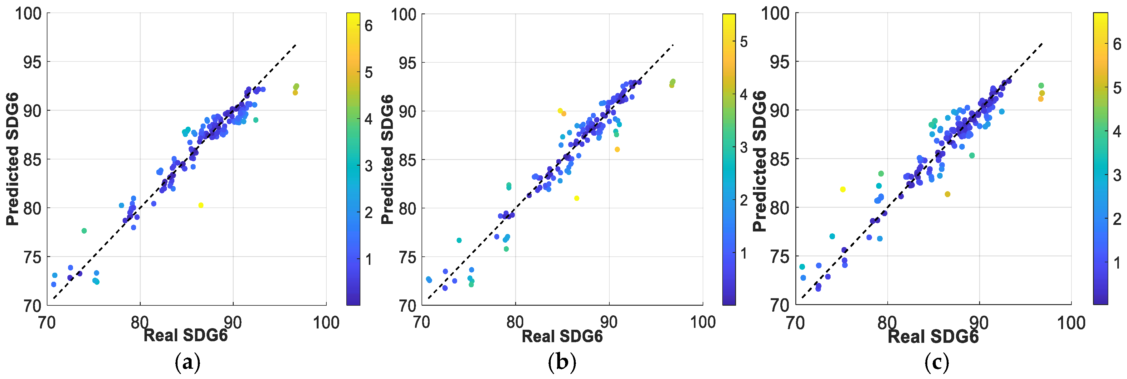
The regression curves of the THRO-optimized BiLSTM-based models for CFDM, EFDM, and RFDM are presented in Figure 2. In each sub-panel, the horizontal axis represents the actual SDG6 values, and the vertical axis represents the model-predicted values; data points are color-coded according to the magnitude of the absolute prediction error.

Data points are color-coded by the magnitude of the absolute prediction error.

Across all three models, the majority of predicted values cluster tightly along the reference line ($y=x$), confirming that the THRO-BiLSTM framework achieves a high overall prediction accuracy in the multi-country time-series setting. However, a comparative examination reveals meaningful qualitative differences among the models.

In CFDM, dark-colored data points, indicating low prediction errors, are prominently concentrated along the reference line, and the distribution of low errors is nearly uniform across the entire prediction range. The compact and balanced dispersion of points around the reference line suggests that the model has developed a consistently stable prediction behavior across a broad SDG6 value range. In EFDM, while overall predictions are generally successful, the color distribution forms a relatively wider band in certain SDG6 value intervals, accompanied by a modest increase in local deviations. In RFDM, the scatter around the reference line is noticeably wider, with brighter color clusters concentrated in the high SDG6 region, suggesting elevated prediction uncertainty at extreme values.

These observations are consistent with the quantitative metrics reported in

Table 3. Comparative prediction performance of the THRO-optimized BiLSTM models for CFDM, EFDM, and RFDM.

Metric	CFDM	EFDM	RFDM
$R^2$	0.9216	0.9155	0.8997
RMSE	1.4465	1.5018	1.6358
MAE	1.0712	1.0747	1.1472

. The $R^2$ values of 0.9216, 0.9155, and 0.8997 for CFDM, EFDM, and RFDM, respectively, align well with the qualitative differences observed in the regression curves. The regression analysis establishes that CFDM not only achieves the highest global accuracy but also demonstrates the strongest prediction stability and generalizability across the full SDG6 value range.

4.2. Country-Level Scatter Analysis

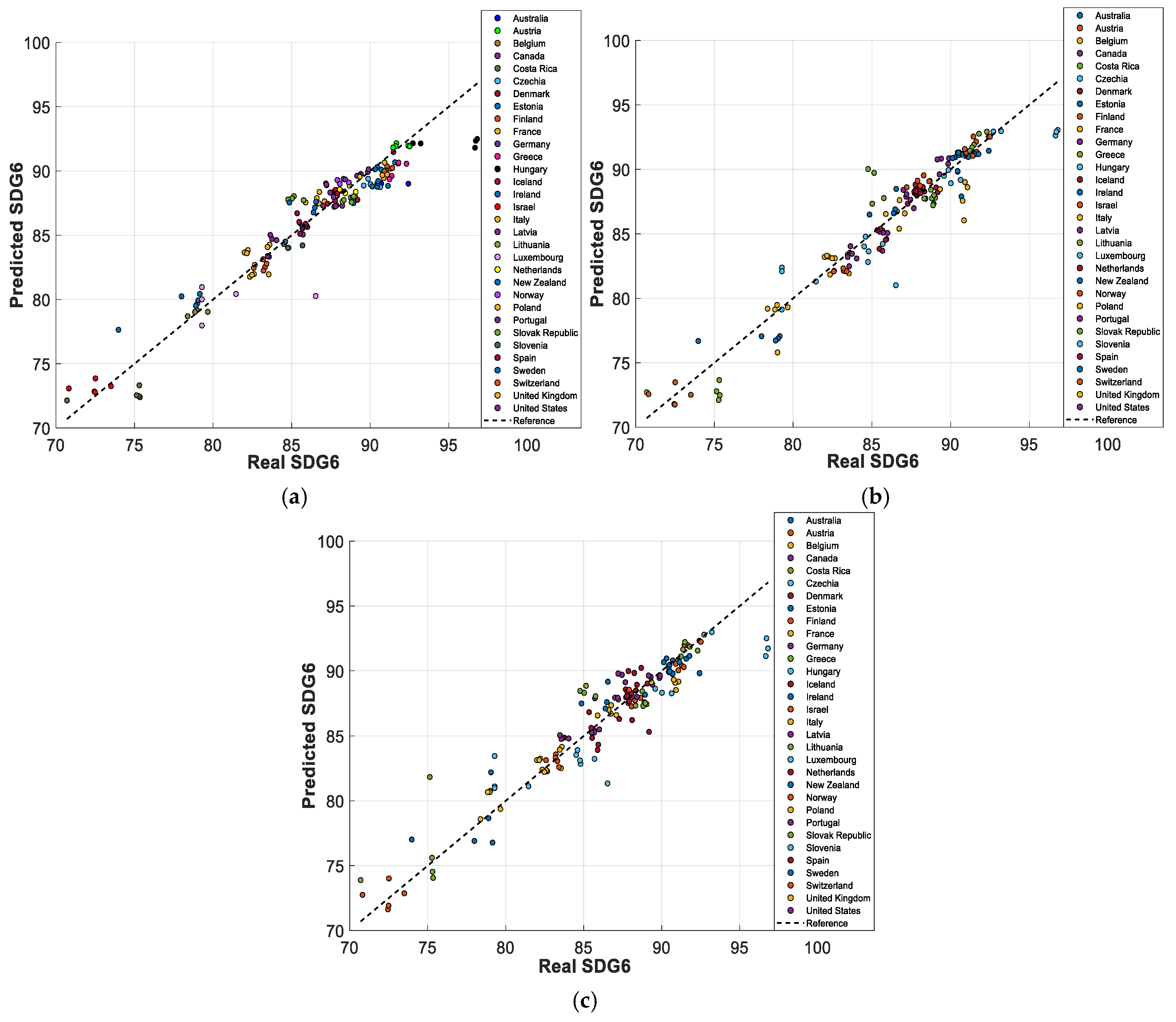
Figure 3 presents the country-level comparison between the SDG6 predictions generated by the THRO-BiLSTM models and the corresponding observed values. Each country is assigned a distinct color, enabling a visual assessment of whether any model exhibits a systematic prediction bias toward specific country profiles. In all three models, the majority of data points concentrate around the reference line, confirming that the THRO-BiLSTM framework exhibits a strong predictive capacity within the multi-country panel structure. However, notable differences emerge among the models upon closer inspection.

In CFDM, country-specific colors are distributed homogeneously along the reference line, with no discernible systematic over- or under-prediction tendency attributable to any particular country group. This finding indicates that the model successfully generalizes across OECD countries with diverse socio-economic and institutional profiles, demonstrating a country-agnostic prediction behavior largely free from country-specific biases.

In EFDM, the color distribution remains broadly balanced; however, a limited number of countries exhibit relatively greater deviations from the reference line. This pattern suggests that the EFD specification is less adept at capturing the structural characteristics of certain country profiles that are better characterized by alternative fiscal dimensions.

In Model RFDM, notable deviations from the reference line are observed for specific countries, particularly in the lower SDG6 range. This pattern implies that the RFD variable is comparatively less capable of explaining the structural heterogeneity prevalent among countries with low sustainability performance. This finding underscores the importance of considering fiscal pressures on water and sanitation services not in isolation through revenue-sharing mechanisms alone, but jointly with institutional capacity, expenditure efficiency, and integrated fiscal architecture.

Overall, the country-level scatter analysis confirms that CFDM exhibits the most balanced and least biased prediction structure across all country profiles.

4.3. Prediction Error Distribution

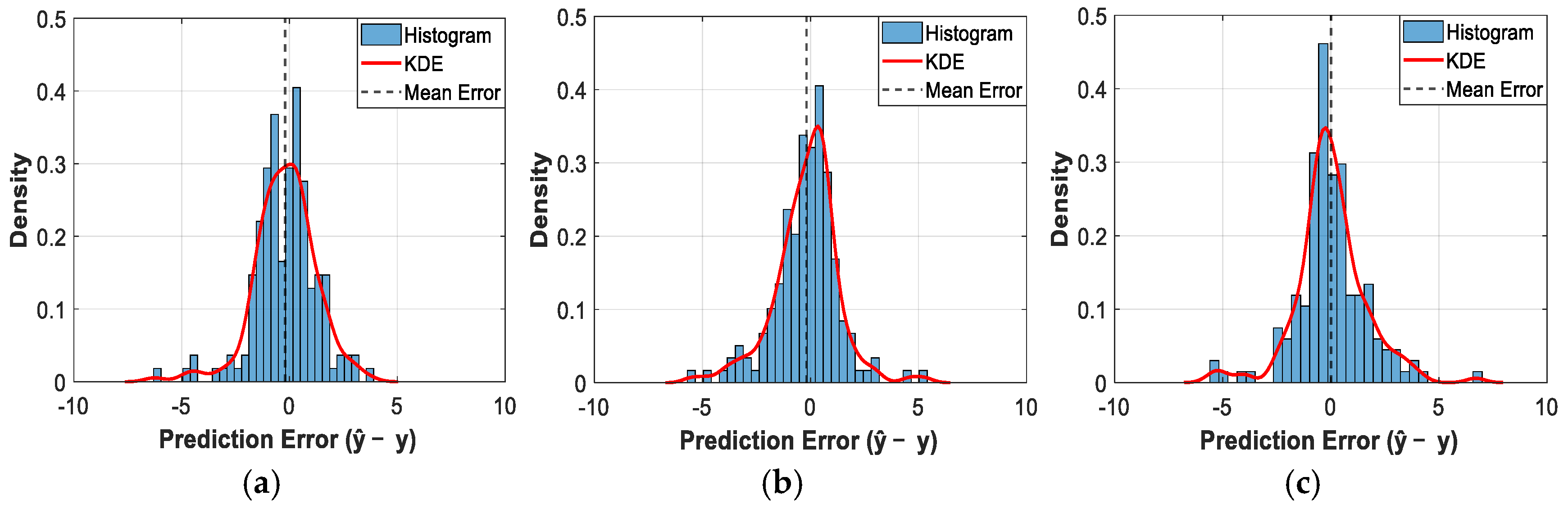
Figure 4 presents a comparative distribution of prediction errors $e=y-\widehat{y}$ for CFDM, EFDM, and RFDM, assessed through both histograms and kernel density estimation (KDE) curves.

Across all three models, prediction errors are concentrated around zero and the mean error is positioned close to the center. This pattern indicates that the THRO-BiLSTM framework is largely free from systematic over- or under-prediction bias, providing a strong foundation for the general validity of the models.

In CFDM, the KDE curve forms a notably sharp peak over zero with markedly limited tails. This high-kurtosis profile indicates that small-to-moderate errors dominate the distribution and that large deviations are extremely rare. This finding demonstrates that CFDM is statistically superior not only in terms of mean accuracy but also with respect to the shape of the error distribution itself.

EFDM also exhibits a symmetric and centrally concentrated error distribution; however, compared to CFDM, the peak of the KDE curve is relatively lower, and the tail regions cover a somewhat wider area. This pattern suggests that, while the overall distribution remains within acceptable bounds, a limited number of observations display elevated prediction uncertainty.

In RFDM, while the error distribution is broadly symmetric, more pronounced deviations in the tail regions indicate increased local prediction uncertainty for certain country-year combinations. The mild asymmetric clustering in the positive tail further suggests the possible presence of systematic under-prediction tendencies for specific observation groups.

Taken together, the error distribution analysis confirms that CFDM provides a more concentrated, narrower, and more symmetric error profile, establishing it as the most reliable model in terms of both statistical stability and practical predictive accuracy.

4.4. Bland–Altman Agreement Analysis

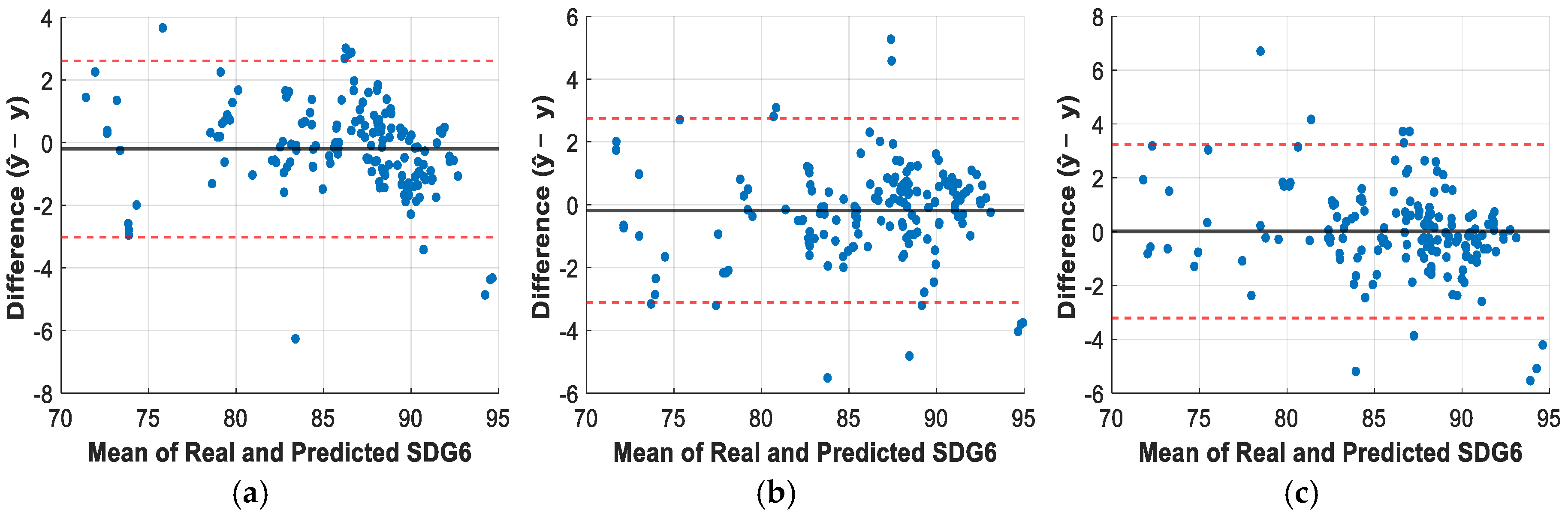
To assess the agreement between predicted and observed SDG6 values not only at the level of correlation but also within a difference-based framework, Bland–Altman analysis was applied. The resulting plots for CFDM, EFDM, and RFDM are presented comparatively in Figure 5. In each panel, the horizontal axis represents the mean of the predicted and observed values $(\widehat{y}+y)/2$, and the vertical axis represents the difference $\widehat{y}-y$. The horizontal dashed lines indicate the mean difference ($\bar{d}$) and the 95% limits of agreement defined as $\bar{d}\pm 1.96\cdot \mathrm{SD}$.

In all three models, the vast majority of observations fall within the 95% limits of agreement, and the mean difference line is positioned close to zero. These findings indicate that the THRO-BiLSTM framework is generally free from pronounced systematic bias, and that prediction errors remain within bounds acceptable for policy evaluation purposes.

A detailed inspection of CFDM reveals that the difference values exhibit a highly homogeneous dispersion around the mean line, with observations remaining within the agreement limits across the entire SDG6 range. The notably limited number of observations near the agreement band boundaries confirms that the model achieves high prediction stability at both low and high SDG6 levels.

In EFDM, while the mean difference line remains close to zero, the scatter increases at extreme SDG6 values, particularly at the lower and upper ends of the distribution. This pattern implies that, although the model produces reliable predictions for intermediate observations, prediction uncertainty is moderately elevated at the extremes.

In RFDM, the limits of agreement widen noticeably in the high sustainability region, with difference values spreading across a broader band. This finding confirms that prediction uncertainty increases for countries with high SDG6 values. The limited representational capacity of RFD variable in capturing the structural transformations of these countries may be a plausible explanation for the observed agreement deterioration.

The Bland–Altman analysis goes beyond global goodness-of-fit metrics to reveal the prediction reliability of each model across the full SDG6 value range. This analysis conclusively confirms that CFDM constitutes the most reliable framework in terms of bias control, agreement stability, and balanced error behavior.

4.5. Year-Based Error Trend Analysis

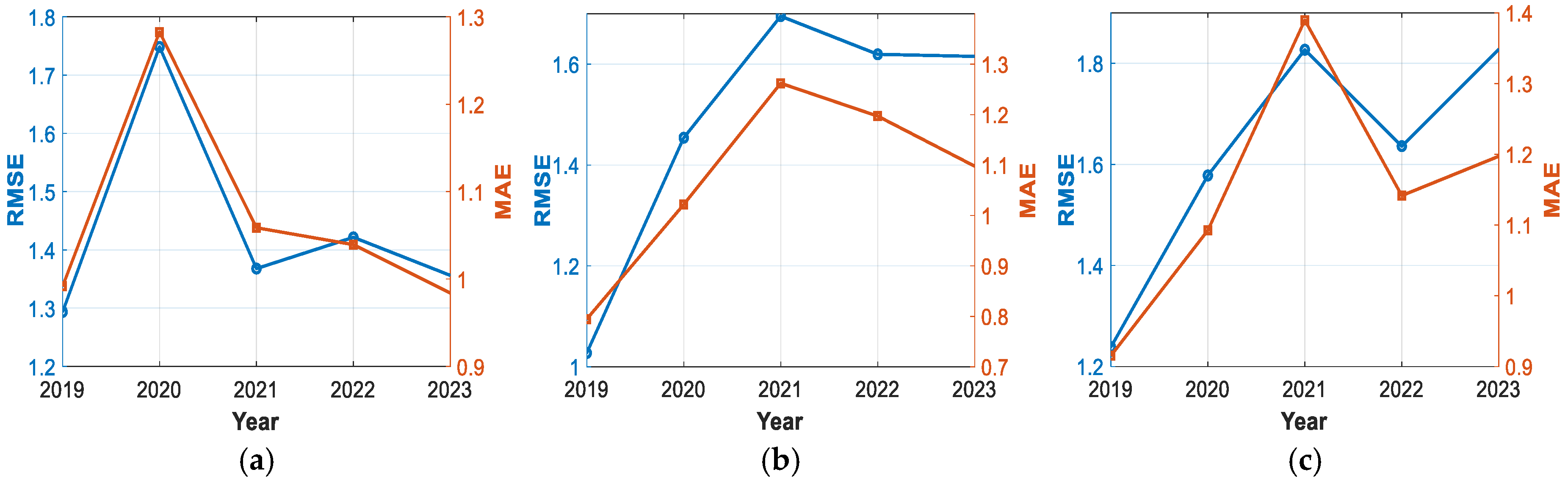
To assess the temporal prediction stability of the models, annual RMSE and MAE values were computed for the 2019–2023 period. The comparative results are presented in Figure 6.

Across all three models, a transient increase in RMSE and MAE values is observed during the 2020–2021 period. This elevation can be directly attributed to the global socio-economic disruptions induced by the COVID-19 pandemic and their structural effects on SDG6 indicators in OECD countries. Factors such as interruptions in water infrastructure investment, reallocation of public expenditures toward immediate health needs, and the temporary contraction of government capacity generated short-term structural breaks in temporal dependency patterns, and transiently degrading prediction accuracy across all models.

CFDM absorbed this structural break with a comparatively limited increase in prediction error. The notable decline in error values observed during the 2022–2023 recovery period indicates that the model successfully adapted to the evolving structural relationships that emerged in the post-pandemic phase. The low learning rate, high hidden-unit capacity, and stronger fully connected layer configuration identified by the THRO algorithm for CFDM can be considered the principal architectural drivers of this temporal flexibility.

EFDM exhibited a similar error elevation during the pandemic period, but with more pronounced fluctuations in certain years. The moderate stabilization of error values in subsequent periods suggests an intermediate level of temporal adaptive capacity.

RFDM displays the highest variance in year-based error changes among the three models. The more irregular error pattern across years and the comparatively slower recovery pace suggest that the RFD specification leads to a more fragile prediction structure in the face of short-term structural changes.

The temporal trend analysis confirms that all three models are applicable for long-term SDG6 forecasting; however, it clearly establishes that CFDM constitutes the superior framework in terms of temporal prediction stability and structural adaptive capacity.

4.6. Overall Prediction Performance

The overall prediction performance of the proposed CFDM, EFDM, and RFDM is comparatively summarized in Table 3. In Table 3, bold values denote the best-performing result for each metric, with higher $R^2$ and lower $RMSE$ and $MAE$ values indicating better predictive performance. The reported results represent the average performance of over 100 independent runs.

Several important findings emerge from Table 3. First, the consistently high $R^2$ values across all three models, with even the weakest model, RFDM, achieving an $R^2$ value of 0.8997, confirm that the THRO-BiLSTM framework provides a robust predictive structure for modeling the SDG6 outcomes in OECD countries. Nevertheless, the observed performance differences indicate that the choice of FD measurement dimension has a meaningful influence on predictive accuracy.

CFDM achieves the best performance across all three metrics, with $R^2=0.9216$, $\mathrm{RMSE}=1.4465$, and $\mathrm{MAE}=1.0712$. These results suggest that the CFD index, which jointly incorporates both expenditure and revenue dimensions, provides the most comprehensive representation of the institutional and fiscal transmission channels through which water and sanitation outcomes are shaped. Since local governments in OECD countries influence SDG6-related service delivery through both expenditure prioritization and independent revenue capacity, the integrated measure appears to capture this multidimensional institutional dynamic more effectively than the single-dimension alternatives.

EFDM also demonstrates strong and consistent predictive performance, with $R^2=0.9155$, $\mathrm{RMSE}=1.5018$, and $\mathrm{MAE}=1.0747$, closely following CFDM. The relative strength of the expenditure-based specification supports the view that local government decisions regarding resource allocation for water infrastructure and sanitation services play a decisive role in SDG6 outcomes. However, the exclusion of the revenue dimension leaves an important informational layer, namely subnational financing capacity, outside the model specification.

RFDM records the weakest performance, with $R^2=0.8997$, $\mathrm{RMSE}=1.6358$, and $\mathrm{MAE}=1.1472$. The relative underperformance of the revenue-based specification suggests that local tax revenues and intergovernmental transfers alone do not provide sufficient explanatory power for predicting water and sanitation performance. This finding is consistent with the broader interpretation that expenditure flexibility, prioritization capacity, and institutional governance quality may influence SDG6 outcomes independently of the overall budgetary capacity of local governments.

Finally, the relatively moderate differences between $RMSE$ and $MAE$ values across all models suggest that the prediction errors are not dominated by extreme deviations. This pattern indicates a broadly balanced error structure and is consistent with the error distribution analysis presented in Figure 4.

4.7. Optimal BiLSTM Hyperparameters Identified by the THRO Algorithm

The optimal BiLSTM hyperparameter configurations identified by the THRO algorithm for each model are presented in

Table 4. Optimal BiLSTM hyperparameters for CFDM, EFDM, and RFDM.

Hyperparameter	CFDM	EFDM	RFDM	Description
Learning Rate	0.0006069	0.00554493	0.000307733	Effective learning rate
Hidden Unit (BiLSTM-1)	160	64	736	First LSTM Layer
Hidden Unit (BiLSTM-2)	448	416	304	Second LSTM Layer
Fully Connected Units	216	40	16	Dense layer size
Batch Size	64	48	32	Mini-batch size
Epochs	187	189	216	Training duration

. The hyperparameter profiles in Table 4 demonstrate that the THRO algorithm adopted distinct optimization trajectories for each model, confirming its capacity to identify discriminating solutions within a high-dimensional hyperparameter space.

For CFDM, the learning rate of 0.0006069 represents the most balanced value among the three models. The preference by THRO for a low yet stable learning rate indicates that the balance between early convergence and generalization capacity is effectively managed throughout the training process. The two-layer BiLSTM structure with 160 and 448 hidden units, with the particularly high capacity of the second LSTM layer, enables temporal dependencies to be learned in a progressively abstract hierarchical manner. The 216-neuron fully connected layer provides a strong projection capacity for translating the temporal representations into the final prediction stage. The batch size of 64 maintains a diversity-efficiency balance in stochastic gradient optimization, while the 187-epoch training duration incorporates an early-stopping approach that limits overfitting.

For EFDM, the selected configuration of 64 and 416 hidden units with a 40-neuron fully connected layer points to a more compact architectural structure relative to CFDM. The relatively high capacity of the second LSTM layer, however, supports the model’s ability to learn long-range temporal dependencies.

The configuration identified for RFDM reveals that THRO followed a distinctly different optimization trajectory. The first LSTM layer comprising 736 units represents the largest representational capacity among the three models, while the 16-neuron fully connected layer constitutes an extremely compact projection stage. Despite this asymmetric architecture, the relatively low $R^2$ of RFDM highlights that network capacity alone is not the decisive factor in determining predictive accuracy; rather, the explanatory power of the independent variables with respect to SDG6 and the adequacy of the variable selection strategy are equally, if not more, critical.

This divergent hyperparameter search behavior of the THRO algorithm demonstrates that it is not merely an optimization routine but an adaptive configuration framework that responds to the unique data structure and variable set of each model. This finding supports the use of THRO as a robust automated hyperparameter optimization tool in SDG-related research and analogous policy-oriented forecasting problems.

4.8. Comparative Analyses of THRO and Particle Swarm Optimization (PSO) Algorithm for SDG6 Prediction

The performance of the BiLSTM-based models with hyperparameters optimized by the THRO and PSO algorithms is comparatively presented in

Table 5. Comparative performance analysis of THRO- and PSO-optimized BiLSTM models for CFDM, EFDM, and RFDM.

Algorithm	CFDM			EFDM			RFDM
	${\mathit{R}}^2$	RMSE	MAE	${\mathit{R}}^2$	RMSE	MAE	${\mathit{R}}^2$	RMSE	MAE
THRO	0.9216	1.4465	1.0712	0.9155	1.5018	1.0747	0.8997	1.6358	1.1472
PSO	0.9022	1.6151	1.1550	0.8868	1.7381	1.3589	0.8887	1.7236	1.2093

using $R^2$, RMSE, and MAE metrics. To ensure a fair and controlled benchmark comparison, both optimization algorithms were evaluated under identical experimental conditions. Specifically, THRO and PSO were tested using the same training and test partitions, the same BiLSTM architecture, the same five-dimensional hyperparameter search space, the same search bounds, the same objective function, and the same deterministic rapid-evaluation strategy. The fitness function was defined as $\mathcal{F}=1-R_{\mathrm{test}}^2$ for both algorithms. In addition, the total search budget was kept identical across the two optimizers. Since THRO uses two sub-populations with $n=5$ agents each, corresponding to ten candidate agents per iteration, the PSO population size was also fixed at ten particles. Likewise, the maximum number of iterations was set to T = 100 for both algorithms, yielding 1000 BiLSTM fitness evaluations per optimization run in each case. Therefore, the comparative results reported in Table 5 reflect differences in the search dynamics and hyperparameter optimization capability of THRO and PSO rather than differences in data partitioning, model architecture, search budget, or computing resources.

For the CFDM, THRO achieved $R^2=0.9216$, $RMSE=1.4465$, and $MAE=1.0712$, whereas PSO obtained $R^2=0.9022$, $RMSE=1.6151$, and $MAE=1.1550$. These results indicate that THRO provides an approximately 2.15% improvement in $R^2$ compared with PSO, while reducing RMSE and MAE by approximately 10.44% and 7.26%, respectively.

For the EFDM, THRO also demonstrates a clear performance advantage over PSO. The $R^2$ value increases from 0.8868 to 0.9155, corresponding to an improvement of approximately 3.24%. Moreover, RMSE decreases from 1.7381 to 1.5018, while MAE decreases from 1.3589 to 1.0747, indicating error reductions of approximately 13.60% and 20.91%, respectively. This result suggests that THRO is particularly effective in optimizing the expenditure-based BiLSTM structure.

A similar trend is observed for the RFDM. THRO improves the $R^2$ value from 0.8887 to 0.8997 and reduces RMSE from 1.7236 to 1.6358 and MAE from 1.2093 to 1.1472. Although the improvement margin is relatively smaller than those observed for CFDM and EFDM, THRO still consistently outperforms PSO across all evaluation metrics.

Overall, when the three models are evaluated together, THRO provides an average R² improvement of approximately 1.97 percentage points compared with PSO. In addition, THRO reduces RMSE by approximately 5.09–13.60% and MAE by approximately 5.13–20.91% across the three model structures. These findings confirm that THRO provides a more effective hyperparameter optimization strategy than PSO for BiLSTM-based SDG6 prediction models.

4.9. Robustness Check: Excluding the COVID-19 Period

As an additional robustness check, the models were re-estimated after excluding the observations corresponding to 2020 and 2021, the two years most severely disrupted by the COVID-19 pandemic. This restricted-sample experiment was designed to examine whether the main model hierarchy and the predictive association between fiscal decentralization measures and SDG6 performance were driven by pandemic-period observations. The same BiLSTM architecture, THRO-based hyperparameter optimization procedure, training strategy, and evaluation metrics were retained in the robustness experiment.

The restricted sample results confirm that the core findings remain substantively stable. After excluding 2020–2021 observations, the CFDM continued to provide the strongest predictive performance, with $R^2=0.9184$, $RMSE=1.4728$, and $MAE=1.0915$. The EFDM also preserved its advantage over the RFDM among the two unidimensional fiscal decentralization specifications, achieving $R^2=0.9098$, $RMSE=1.5486$, and $MAE=1.1194$. By comparison, the RFDM recorded $R^2=0.8935$, $RMSE=1.6822$, and $MAE=1.1896$. These results indicate that the superior performance of the composite fiscal decentralization model is not driven solely by the pandemic-period observations. More importantly, the ranking of the three model specifications remains unchanged, with CFDM outperforming EFDM and RFDM, thereby confirming that the balance between subnational expenditure responsibilities and revenue capacity provides the most informative fiscal signal for SDG6 prediction.

4.10. Integrated Comparative Discussion

The integrated evaluation of regression analysis, country-level scatter patterns, error distributions, Bland–Altman agreement analysis, year-based error trends, the restricted-sample robustness check, and overall performance metrics reveals that the differences among the three models form a coherent and theoretically meaningful pattern across both statistical and policy interpretation dimensions.

First and foremost, the fact that all three models achieve $R^2>0.89$ confirms that the THRO-BiLSTM framework is capable of learning the temporal patterns of SDG6 components in OECD countries with high accuracy. This finding aligns with the growing body of literature demonstrating that deep learning architectures can be successfully adapted to the forecasting of social policy indicators.

RFDM, with $R^2=0.8997$, $RMSE=1.6358$, and $MAE=1.1472$, delivers the weakest performance among the three models. The increasing error structure at low-to-medium SDG6 levels and the higher variance in year-based error changes suggest that the RFD dimension alone is insufficient to reflect the institutional transmission channels through which water and sanitation services are shaped. This finding supports the theoretical frameworks arguing that local revenue capacity becomes determinative for SDG6 outcomes only when jointly considered with expenditure flexibility, infrastructure investment, and institutional governance quality.

EFDM, with $R^2=0.9155$, $RMSE=1.5018$, and $MAE=1.0747$, delivers a strong and balanced performance. The relative strength of the expenditure-based specification supports the view that local governments’ direct allocation decisions toward water infrastructure and sanitation play a meaningful role in shaping SDG6 outcomes. Nevertheless, the increased scatter at extreme values in the Bland–Altman analysis and the year-based prediction fluctuations indicate that this model exhibits comparatively limited stability under certain conditions relative to CFDM.

CFDM, with $R^2=0.9216$, $RMSE=1.4465$, and $MAE=1.0712$, emerges as the superior framework across all evaluation metrics. Three interrelated factors underlie this performance advantage. First, the CFD index jointly incorporates both expenditure and revenue dimensions, providing the richest institutional representation of the fiscal channels through which water and sanitation services are shaped. Second, the hyperparameter configuration identified by THRO for CFDM, a low learning rate, high hidden-unit capacity, and a stronger fully connected layer, establishes an optimal equilibrium between learning stability and representational power. Third, the rich informational environment created by the composite variable set enables the bidirectional temporal learning mechanism of the BiLSTM to capture more complex dependency patterns, directly reinforcing the model’s temporal stability.

Although the present study uses the aggregate SDG6 index as the dependent variable, the multidimensional structure of SDG6 suggests that EFDM, RFDM, and CFDM may be associated with different subcomponents through distinct channels. EFDM can be expected to be particularly relevant for infrastructure-intensive dimensions such as drinking-water access, sanitation facilities, wastewater treatment, and maintenance of water-related infrastructure, because these areas depend directly on local budget allocation, capital expenditure, procurement capacity, and operational spending discretion. RFDM may be more strongly related to the financial sustainability of service provision, especially where local governments rely on own-source revenues, user charges, and predictable revenue streams to sustain routine operation and maintenance. CFDM is theoretically expected to be more informative for sub-dimensions requiring both investment discretion and stable financing, such as water-quality management, integrated water-resource governance, and resilience-oriented service continuity. Therefore, the superior predictive performance of CFDM at the aggregate level is consistent with the theoretical expectation that SDG6 achievement requires not only expenditure authority or revenue capacity in isolation, but an institutional balance between the two. Future studies could extend this analysis by separately estimating SDG6 sub-indicators to test whether these theoretically expected differences are empirically observed across water access, sanitation, wastewater, water scarcity, and ecosystem-related components.

The present findings are broadly consistent with the core literature linking decentralization, local fiscal capacity, and sustainability-related outcomes, while also extending this literature in several important ways. Similar to previous studies, the results suggest that fiscal decentralization and local fiscal capacity are positively associated with water, sanitation, and sustainability performance. However, the present study moves beyond earlier evidence by focusing directly on SDG6 rather than broader development or general SDG outcomes. It also differs from municipal-level single-country analyses by providing comparative evidence from an OECD panel. More importantly, the study evaluates EFDM, RFDM, and CFDM within the same predictive framework and shows that RFDM alone is less informative than CFDM in predicting aggregate SDG6 performance. In this respect, the paper contributes to the literature by isolating SDG6 as a specific water–sanitation governance outcome, distinguishing alternative fiscal decentralization metrics, introducing CFDM as a balance-oriented fiscal signal, and combining THRO-optimized BiLSTM prediction with GRA-based relational interpretation.

These findings are consistent with comparative analysis literature showing that composite measurement approaches in FD research provide stronger explanatory power than one-dimensional metrics. Furthermore, they reinforce the conclusion that in AI-enabled SDG forecasting studies, the design of the variable set is at least as determinative of model performance as the choice of network architecture.

The results of the model performance confirm the high predictive capacity of the AI-based method, and the further analysis of the directional effects and the relative impact shares of the variables allows for a more complete interpretation of the fiscal, socio-economic and institutional dynamics that influence the performance of SDG6. Therefore, the directional effects of the variables were first identified by the average coefficients resulted from the 100-iteration convergence process. Then, a multi-criteria decision-making (MCDM) method was used to compute the integrated impact levels of the variables on SDG6 across the three models. As one of the MCDM methods, the reciprocal approach was used to determine the relative priorities of the models, considering the multiple criteria in the ranking of the impact intensities of the variables. The weighting results, in determining indexes of impact intensities of the variables, computed by the model performance indicators ($R^2$, $MAE$ and $RMSE$) were reported as w values in

Table 6. Directional effects and variable impact shares.

A: Coefficients
	FD	DUMMY	GDP	POP	URB	GOV
CFDM	0.2433	−0.3132	−0.2538	0.0716	−0.4862	0.2754
EFDM	0.3769	−0.2834	−0.2760	−0.0190	−0.3928	0.1455
RFDM	0.2311	−0.2784	−0.2102	0.0633	−0.4493	0.2669
B: Model performance indicators and w
		$R^2$	MAE	RMSE	w
	CFDM	0.9147	1.1182	1.5032	0.4260
	EFDM	0.9090	1.1190	1.5581	0.3611
	RFDM	0.8930	1.2147	1.6899	0.2130
C: GRA-based variable impact shares and index rankings
	FD	DUMMY	GDP	POP	URB	GOV	TOTAL
CFDM	0.1483	0.1898	0.1539	0.0465	0.2949	0.1666	1.000
EFDM	0.2528	0.1894	0.1847	0.0131	0.2626	0.0974	1.000
RFDM	0.1547	0.1856	0.1401	0.0421	0.2999	0.1775	1.000
Index	0.6305	0.5712	0.5169	0.3333	1.0000	0.4741
Rank	2	3	4	6	1	5

Note. The distributions of the coefficients in all models, belonging to 100 iteration series (18 series), were examined using Shapiro–Wilk normality distributions. It was determined that all distributions were not normally distributed at a statistical significance level of 0.001. The one-sample t-test and its equivalent non-parametric Wilcoxon signed-rank test strongly indicated that the coefficients for all 18 series are non-zero, at a statistical significance level of 0.001. Thus, it is concluded that all coefficients in Table 6 are statistically significant and are factors affecting SDG6.

. Therefore, the models’ contributions to the integrated impact calculations were weighted by their performance levels. The results show that the CFDM has the highest weight in the integrated impact calculations, which is 42.6%. Following the weighting procedure, Grey Relational Analysis (GRA) was employed to identify the relative temporal association shares of the variables. At this stage, it is important to clarify the conceptual boundary between the THRO-BiLSTM model and the GRA procedure. The THRO-BiLSTM model constitutes the main predictive architecture of the study and is used to learn nonlinear temporal dependencies between fiscal, socio-economic, institutional variables and SDG6 outcomes. By contrast, GRA is not used to extract variable importance directly from the internal parameters, gates, hidden states, gradients, or learned representations of the BiLSTM network. Instead, it is employed as a complementary post-estimation relational analysis that evaluates the degree of similarity and association between each normalized explanatory series and the SDG6 reference series. Therefore, the GRA-based rankings should be interpreted as temporal relational association scores rather than neural-network-derived feature-importance values.

GRA is a popular MCDM technique that measures the degree of similarity and association between reference and comparative series. According to Yin (2013), GRA has been extensively applied in ISI-indexed studies and is considered an effective approach, particularly under conditions of insufficient information, large datasets, and uncertainty [103]. The method has also been applied in a variety of areas, such as stock selection [104], optimization processes [105], and sales forecasting [106]. In panel time-series applications, GRA offers several advantages because it is scale-free after normalization, does not require strict distributional assumptions, performs well under limited and heterogeneous information structures, and provides an interpretable way to compare the relative closeness of multiple variables to a reference outcome. Within this framework, the variable indexes obtained from GRA were evaluated as complementary relational association magnitudes across the three models, while the predictive accuracy and generalization capacity of the study remained assessed through the THRO-optimized BiLSTM framework.

The findings regarding coefficient directions and variable impact shares are presented in Table 6.

The positive coefficients of the CFD, EFD, and RFD variables across all models indicate that FD is positively associated with SDG6 and the ranking of the coefficient magnitudes, EFD (0.3769) > CFD (0.2433) > RFD (0.2311), suggests that the relationship is particularly strong in terms of local expenditure capacity. This finding is consistent with the core principle of fiscal federalism theory that local decision-making authority and resource allocation will improve service effectiveness [25]. The positive coefficient of the RFD model indicates that local revenue-generating capacity contributes to water and sanitation outcomes by supporting local service delivery. Meanwhile, the positive impact found for CFD supports the idea that the combined performance of the revenue and expenditure mechanisms is more comprehensive for the SDG6 performance. However, the relatively higher coefficient obtained for EFD means that, as theory predicted, the expenditure authority and the effective use of local spending capacity are more decisive in application- and infrastructure-intensive sectors such as water and sanitation. This stronger association can be explained by some of the institutional and service delivery mechanisms. Water and sanitation services are essentially local public services, and require ongoing maintenance, operation and investment in infrastructure. Greater discretion over local spending may therefore allow subnational governments to allocate resources more efficiently to meet local needs and service priorities, improving the responsiveness and effectiveness of service delivery. Expenditure autonomy could also bring about more flexible infrastructure planning and quicker responses to local challenges related to water supply, wastewater management and system maintenance. Local governments are usually closer to the users of services and decentralization of expenditure decisions may also improve accountability and ensure a better match between public expenditures and community needs. These mechanisms are generally compatible with theoretical arguments of FD that stress the advantages of local information and the efficiency gains from matching public expenditures with local preferences. Although this study does not directly test these transmission channels, the stronger association of EFD suggests that local spending authority could be an important governance mechanism to improve SDG6 outcomes.

These findings imply that FD is not only about fiscal autonomy but also about improving the efficiency of service delivery through local decision-making and implementation capacity. In particular, the ability of local authorities to set expenditure priorities in accordance with regional needs may enable a more efficient allocation of resources, especially in sectors with high infrastructure intensity and a strong dependence on public services. Furthermore, the use of an OECD sample shows that FD is not only a policy instrument for developing countries, but also an important determinant of service performance in economies with relatively high institutional capacity.

The findings indicating the positive contribution of FD to SDG6 are broadly consistent with the limited but growing literature emphasizing the role of decentralized fiscal structures in water, sanitation, and sustainability outcomes. Although the existing empirical evidence remains relatively fragmented and indirect, previous studies generally suggest that stronger local fiscal capacity enhances service delivery performance and sustainability-oriented public outcomes. In particular, the positive effects identified for all models of FD are compatible with the findings of Taiwo (2024), who reported that both expenditure and revenue decentralization improve access to water and sanitation within the MDG framework [82]. While that study did not directly focus on SDG6, the consistency of the findings suggests that decentralized fiscal structures may improve water and sanitation performance through stronger alignment between local needs and public resource allocation. The comparatively stronger performance of the EFDM in this study further supports the argument that water and sanitation services are highly dependent on local expenditure capacity, infrastructure investment, and operational service delivery. Similarly, the positive contribution of RFDM identified in the present analysis is broadly aligned with the findings of Martínez-Córdoba et al. (2020), who found that local government revenues and water-related taxes positively affect SDG6 performance in Spain [60]. Although local revenues do not directly represent FD in a comprehensive sense, they reflect local fiscal capacity and therefore support the broader theoretical argument linking local financial autonomy to sustainable water and sanitation outcomes. The findings are also indirectly supported by Benito et al. (2025), who demonstrated that municipalities characterized by weak fiscal capacity and lower tax revenue collection exhibit lower SDG compliance [83]. This relationship reinforces the idea that local fiscal strength constitutes an important enabling factor for sustainable development performance. However, the evidence reported by Benito et al. (2023), indicating that higher SDG alignment may weaken municipal budget balances and fiscal capacity, also suggests that achieving sustainability goals may generate additional fiscal pressures on local governments [39]. In this respect, the present findings imply that the positive contribution of FD to SDG6 may depend not only on fiscal autonomy itself, but also on the fiscal sustainability of local governments. Finally, the positive relationship identified between FD and SDG6 is also broadly compatible with the findings of Gariba et al. (2024), who reported that FD contributes positively to the social and environmental dimensions of the SDGs in OECD countries [24]. Given the strong environmental dimension of SDG6, the present findings further reinforce the argument that decentralized fiscal structures may facilitate environmentally sustainable public service delivery. Unlike the existing literature, however, this study comparatively evaluates composite, expenditure-, and revenue-based FD structures within an AI-supported analytical framework while also integrating coefficient directions and variable impact rankings. Therefore, the study extends the existing literature by providing a more comprehensive interpretation of how fiscal, socio-economic, and institutional dynamics jointly shape SDG6 performance.

DUMMY, as a proxy for government structure, also exhibits a negative coefficient. This finding, reflecting the federal–unitary distinction, implies that the distribution of authority across multiple governmental levels may generate coordination challenges, limit economies of scale, and reduce the effective management of cross-border externalities. This interpretation is consistent with the literature suggesting that government structure systematically influences local government behavior and public service delivery [107]. On the other hand, the negative coefficient of GDP may be related to the structural characteristics of the OECD sample, where water and sanitation infrastructure systems are already widely installed and industrial production, urban consumption patterns and environmentally intensive economic activities continue to exert additional ecological pressures. This result differs from the positive relationship found by Roy and Pramanick (2019) in a sample of developing countries [4]. Population dynamics also appear to play a significant role in shaping SDG6 performance. The model-specific variation observed for the POP variable is also consistent with studies indicating that the impact of population growth on water and sanitation outcomes is not unidirectional [77,79]. The negative coefficient of POP within the EFDM may reflect the increasing infrastructure and expenditure pressures generated by population growth in service-intensive sectors such as water and sanitation. Conversely, the positive coefficients identified in the CFDM and RFDM frameworks suggest that stronger local fiscal capacity may help mitigate population-related service pressures. Closely related to population dynamics, URB also emerges as a critical factor shaping SDG6 performance across the three models. The negative coefficient of the URB in all models suggests that the increased population density, water demand and environmental pressures particularly in OECD countries have placed significant stress on infrastructure systems. This result is consistent with Teixeira de Mello et al. (2024) who showed that URB has negative effects on water quality [78]. However, this is inconsistent with the findings of Bao and Chen (2017) who argued that URB can increase water use efficiency [76]. This discrepancy implies that the effect of URB may vary depending on the particular indicator considered. These infrastructure and coordination intensive pressures also imply that the sustainability of water and sanitation services is not only a matter of fiscal capacity, but also of the effectiveness of governance and institutional coordination mechanisms. The positive effect of GOV is consistent with studies emphasizing the importance of institutional coordination and multi-level governance structures for the sustainability of water and sanitation services [63,64,65,66,67].

The coefficient interpretations and literature-based discussions indicate the directional relationships between variables and SDG6 performance, while the GRA-based index and ranking results provide a wider comparative perspective for the relative influence levels of variables across the overall modeling framework. The ranking results suggest that the urbanization pressures are the most major contributor in shaping the SDG6 performance in the OECD sample. The highest impact level of the URB variable indicates that the increase in population density, the increase in water demand, the burden of infrastructure and the pressure on the environment play a decisive role in water and sanitation systems. This finding suggests that water and sanitation challenges in OECD countries are not only about access but are also increasingly about wider structural issues such as sustainable infrastructure management, controlling environmental pressures and the long-term sustainability of service provision. The second ranking of FD underscores the persistent importance of local fiscal capacity and decentralized decision-making authority for effective water and sanitation services. While infrastructure investments have been largely completed across OECD countries, local fiscal flexibility remains an important determinant in infrastructure maintenance, renewal, service quality enhancement and environmental compliance processes. The DUMMY variable, representing government structure, comes third in line, indicating that the differences in institutional coordination between federal and unitary systems create important implications for the SDG6 performance. This implies that the coordination capacity of multi-level governance systems is a key factor for the sustainability of water and sanitation services. The fourth position of GDP suggests that economic growth is not irrelevant for SDG6 performance, but its marginal contribution may be relatively limited in OECD countries because of infrastructure saturation and growing environmental pressures. While the GOV variable exhibits a positive effect, its relatively lower magnitude may be associated with the existence of a threshold level of governance quality in the countries of the OECD. Therefore, although governance remains an important enabling factor for SDG6 performance, the findings suggest that the key differentiating dynamics are urbanization pressures and fiscal capacity. Finally, the relatively low impact level of the POP variable indicates that the spatial concentration of population, i.e., urbanization, is a more decisive factor for SDG6 performance than the total size of the population itself.

Additionally, a radar plot is presented in Figure 7 to further illustrate the relative impact levels of the variables across the CFDM, EFDM, and RFDM frameworks. The radar plot provides a more integrated visualization of the comparative impact structures identified through the GRA-based rankings and coefficient findings.

Figure 7 displays a visual validation of the impact structures with respect to the coefficient results and the rankings by GRA. The radar plot shows a strong influence of URB on all model structures, which means that infrastructure pressure, population concentration and environmental stress are important factors determining the SDG6 performance. The figure also suggests that the impact of FD is stronger under the EFDM framework, supporting the argument that local expenditure capacity is particularly important in infrastructure- and service-intensive sectors such as water and sanitation. By contrast, GOV and POP show relatively low and stable levels of impact across the three models. The overall similarity between the CFDM and RFDM structures suggests that integrated fiscal capacity and revenue-based mechanisms lead to relatively similar patterns of impact. Overall, the radar plot underscores the multidimensional nature of SDG6 performance, reflecting the combined influence of fiscal, socio-economic and institutional dynamics.

5. Conclusions and Future Research

Water and sanitation infrastructure is built, operated, and maintained at the local level, yet the fiscal preconditions that make sustained local delivery possible have attracted surprisingly little empirical attention in the SDG literature. This paper took this gap as its starting point. Working with a panel of OECD countries and a hybrid BiLSTM-THRO estimation architecture, we examined how different ways of measuring FD relate to cross-country variation in SDG6 scores, and what the predictive superiority of one specification over another can tell us about the underlying governance mechanisms.

Three findings stand out. To begin with, the CFD index, constructed to reflect the balance between a jurisdiction’s spending authority and its own-source revenue base, proved to be the strongest predictor of SDG6 outcomes in every diagnostic dimension we employed. The gap between CFDM and its unidimensional alternatives is not merely statistical; it carries a substantive message. Local governments that control significant expenditure shares but lack commensurate revenue autonomy, or that enjoy revenue capacity without discretionary spending power, appear less effective at translating fiscal resources into water and sanitation service quality. The two dimensions are not substitutes; they are complements, and policy designs that strengthen one while neglecting the other will likely fall short of their intended effects on SDG6 outcomes.

The second finding concerns the relative weight of the two unidimensional proxies. Across all models and all diagnostic lenses, the expenditure-based specification outperformed the revenue-based one by a consistent margin. This asymmetry makes practical sense: the ability to commission infrastructure, contract maintenance services, and sustain operational budgets depends on spending discretion, not on the formal assignment of revenue sources. A local government that receives generous intergovernmental transfers but has limited say over how those funds are deployed faces a governance constraint that no revenue figure can fully capture. The results suggest that analytical frameworks focusing exclusively on the revenue side of decentralization understate the fiscal determinants of water and sanitation performance.

Third, the year-by-year error decomposition exposed a consistent pattern across all three models: prediction accuracy deteriorated during 2020–2021 before recovering sharply by 2023. That trajectory maps directly onto the COVID-19 disruption and its aftermath. What distinguishes the models is the speed and completeness of that recovery. CFDM adapted to the post-pandemic structural shift more quickly, suggesting that the richness of the composite index allowed BiLSTM to re-anchor its temporal representations as normalized institutional conditions. This is a practical argument for composite measurement: in periods of macroeconomic stress, when individual fiscal indicators may move in disconnected directions, an integrated index preserves more of the signal.

Apart from the strong predictive performance of the three AI-based models, the integrated results based on the coefficient directions and GRA-based impact rankings show that FD is among the major determinants affecting the SDG6 performance of the OECD countries. The coefficient results suggest a broadly positive link between FD and SDG6 performance across all model forms. The integrated impact rankings further highlight that FD is one of the most significant financial dimensions shaping sustainable water and sanitation outcomes.

Overall, the findings provide a strong policy rationale for considering FD as a governance tool to improve SDG6 outcomes, rather than just a fiscal arrangement. Assigning expenditure responsibilities to subnational governments without adequate and predictable own-source revenues, or vice versa expanding revenue authority without adequate expenditure discretion, creates institutional mismatches that may undermine SDG6 performance. The higher performance of the CFDM suggests that expenditure assignments and revenue autonomy should be designed as complementary rather than as independent dimensions of decentralization policy. The results indicate that the largest improvements in SDG6 performance are likely to be found where local governments have both sufficient spending authority and fiscal capacity to support these responsibilities. The policy implications also differ across institutional settings. The negative coefficient and the relatively high impact ranking of the federalism dummy variable suggest that coordination capacity is an important fiscal correlate of SDG6 performance in multi-level governance systems. In federal countries, where responsibilities are divided between several layers of government, the importance of strengthening intergovernmental coordination mechanisms, promoting integrated river-basin management frameworks, improving information sharing systems, and developing joint infrastructure planning arrangements should be considered as key policy priorities. On the other hand, unitary systems may be better served by increasing discretion of local governments over local spending, by reducing administrative constraints on investment decisions at the local level, and by enhancing the predictability of intergovernmental transfers for water and sanitation services. Among the two single-dimensional measures of FD, EFD consistently performed better than RFD, indicating the importance of local expenditure discretion for SDG6 outcomes. This finding suggests that the benefits of decentralization are not distributed equally across all SDG6-related expenditure categories. Decentralized decision-making is especially appropriate for localized investments like water distribution networks, wastewater collection and treatment systems, infrastructure maintenance, leakage reduction programs, rural water services and water quality monitoring, which are highly dependent on local needs, geographic conditions, and service delivery priorities. In contrast, large scale strategic infrastructure projects and cross-jurisdictional water resource management may still need to be centrally coordinated and overseen more closely. The broader set of findings also has important policy implications. Given the negative impacts of economic growth and urbanization, the challenge in the OECD context is no longer how to extend basic access to water and sanitation services, but how to ensure the sustainability of existing infrastructure systems in the face of growing environmental and demographic pressures. Therefore, not just new infrastructure investments, but also the modernization of aging water networks, the development of climate-resilient infrastructure, and the long-term planning mechanisms that can cope with increasing urban water demand are areas policymakers need to focus on. Investment strategies must also be in line with demographic trends: population growth can put considerable strains on water and sanitation systems, especially in urban areas where services are intensive. Moreover, the positive impact of good governance implies that the effectiveness of FD is linked not only to the allocation of fiscal resources but also to the institutional capacity to manage those resources effectively. Reforms to improve SDG6 outcomes should therefore be complemented by measures to strengthen transparency, accountability, performance monitoring systems and intergovernmental coordination mechanisms. At the same time, policymakers need to recognize that the gains from decentralization can be circumscribed by unequal local administrative and fiscal capacity. To address these disparities, decentralization reforms should be supported by equalization transfer systems, targeted infrastructure grants, technical assistance programs, capacity-building initiatives and performance-based funding mechanisms. Such complementary measures can help to ensure that weaker local governments can translate fiscal autonomy into effective water and sanitation outcomes, thereby reducing the risk of increasing territorial inequalities in SDG6 performance. In general, the results indicate that sustainable improvements in water and sanitation performance require an integrated approach combining fiscal autonomy, expenditure responsibility, institutional quality and adaptive infrastructure governance rather than relying on FD alone. Reforms that focus on just one dimension of FD are more likely to generate less sustainable SDG6 results than policies that concurrently enhance local revenue generation, expenditure discretion, governance capacity, and intergovernmental coordination.

Several limitations bound the scope of our conclusions. The analysis covers OECD countries exclusively, a sample defined by relatively high institutional quality and income levels. Whether the relationships identified here hold in lower-income or institutionally weaker settings is an open empirical question that cannot be settled by extrapolation. The reliance on the aggregate SDG6 index also means that heterogeneous effects across its constituent sub-indicators, drinking water, sanitation, wastewater treatment, water quality, remain unexamined. Furthermore, the analysis does not explicitly consider environmental factors, such as water resource endowments and climatic conditions, which may also affect SDG6 performance across countries. Finally, although the BiLSTM-THRO framework delivers strong predictive performance, deep learning models impose limits on causal attribution that traditional econometric approaches do not.

Given the predictive design of the study, the findings should be interpreted as robust predictive associations rather than causal estimates. The THRO-BiLSTM framework identifies which fiscal decentralization specification provides the strongest predictive signal for SDG6 performance, while the supplementary coefficient-based and GRA-based analyses provide additional evidence on directional and relational patterns. Accordingly, the results do not imply that fiscal decentralization mechanically causes improvements in SDG6 outcomes; rather, they show that balanced fiscal decentralization, particularly when revenue capacity and expenditure responsibility are jointly considered, is consistently associated with stronger SDG6 performance across the OECD panel.

Future work might address each of these constraints in turn. Extending the estimation framework to middle- and low-income country panels would test the generalizability of the FD-SDG6 relationship under different institutional conditions. Decomposing the SDG6 index into its sub-indicators would permit a more granular mapping of which fiscal channels matter most for which dimensions of water governance. On the methodological side, integrating attention-based transformer architectures or explainability tools into the estimation pipeline could recover some of the interpretive depth that deep learning currently sacrifices for predictive power. Finally, it would be worth exploring how FD interacts with climate adaptation capacity, digitalization of public services, and subnational governance quality in jointly determining long-run water and sanitation outcomes, questions that sit at the frontier of both sustainable development research and fiscal federalism theory.

References

1. Guerrant, R.L.; DeBoer, M.D.; Moore, S.R.; Scharf, R.J.; Lima, A.A.M. The Impoverished Gut—A Triple Burden of Diarrhoea, Stunting and Chronic Disease. Nat. Rev. Gastroenterol. Hepatol. 2013, 10, 220–229. [Google Scholar] [CrossRef] [Scilit] [PubMed]
2. Ait-Kadi, M. Water for Development and Development for Water: Realizing the Sustainable Development Goals (SDGs) Vision. Aquat. Procedia 2016, 6, 106–110. [Google Scholar] [CrossRef] [Scilit]
3. UN-Water Sustainable Development Goal 6 Synthesis Report on Water and Sanitation; United Nations: New York, NY, USA, 2018.
4. Roy, A.; Pramanick, K. Analysing Progress of Sustainable Development Goal 6 in India: Past, Present, and Future. J. Environ. Manag. 2019, 232, 1049–1065. [Google Scholar] [CrossRef] [Scilit] [PubMed]
5. United Nations General Assembly Resolution 64/292: The Human Right to Water and Sanitation; United Nations: New York, NY, USA, 2010.
6. Guppy, L.; Mehta, P.; Qadir, M. Sustainable Development Goal 6: Two Gaps in the Race for Indicators. Sustain. Sci. 2019, 14, 501–513. [Google Scholar] [CrossRef] [Scilit]
7. Biswas, A.K. Urban Water Security for Developing Countries. River 2022, 1, 15–24. [Google Scholar] [CrossRef] [Scilit]
8. WHO. Progress on Household Drinking Water, Sanitation and Hygiene 2000–2022: Special Focus on Gender; WHO and UNICEF: Geneva, Switzerland, 2023; Available online: https://washdata.org/reports/jmp-2025-wash-households (accessed on 15 April 2026).
9. Mattos, K.J.; Mulhern, R.; Naughton, C.C.; Anthonj, C.; Brown, J.; Brocklehurst, C.; Brooks, C.; Desclos, A.; Escobedo Garcia, N.E.; Gibson, J.M.; et al. Reaching Those Left behind: Knowledge Gaps, Challenges, and Approaches to Achieving SDG 6 in High-Income Countries. J. Water Sanit. Hyg. Dev. 2021, 11, 849–858. [Google Scholar] [CrossRef] [Scilit]
10. Nkiaka, E.; Bryant, R.G.; Okumah, M.; Gomo, F.F. Water Security in sub-Saharan Africa: Understanding the Status of Sustainable Development Goal 6. WIREs Water 2021, 8, e1552. [Google Scholar] [CrossRef] [Scilit]
11. Herrera, V. Reconciling Global Aspirations and Local Realities: Challenges Facing the Sustainable Development Goals for Water and Sanitation. World Dev. 2019, 118, 106–117. [Google Scholar] [CrossRef] [Scilit]
12. Pereira, M.A.; Marques, R.C. Sustainable Water and Sanitation for All: Are We There Yet? Water Res. 2021, 207, 117765. [Google Scholar] [CrossRef] [Scilit] [PubMed]
13. Schmohl, M.; Gunes, B.N.; Turkan, G.; Sennaroglu, B. Ranking the Organisation for Economic Co-Operation and Development (OECD) Countries According to Compatibility to Sustainable Development Goal 6. Sustain. Water Resour. Manag. 2025, 11, 130. [Google Scholar] [CrossRef] [Scilit]
14. Weststrate, J.; Dijkstra, G.; Eshuis, J.; Gianoli, A.; Rusca, M. The Sustainable Development Goal on Water and Sanitation: Learning from the Millennium Development Goals. Soc. Indic. Res. 2019, 143, 795–810. [Google Scholar] [CrossRef] [Scilit]
15. Al-Noaimi, M.A. SDG Goal 6 Monitoring in the Kingdom of Bahrain. DWT 2020, 176, 406–427. [Google Scholar] [CrossRef] [Scilit]
16. Perry, B.; Diprose, K.; Taylor Buck, N.; Simon, D. Localizing the SDGs in England: Challenges and Value Propositions for Local Government. Front. Sustain. Cities 2021, 3, 746337. [Google Scholar] [CrossRef] [Scilit]
17. United Nations Transforming Our World: The 2030 Agenda for Sustainable Development; United Nations: New York, NY, USA, 2015.
18. Seelajaroen, R.; Jitmaneeroj, B. Interdependencies among SDGs: Evidence-Based Insights for Sustainable Development Indicators and Policy. Environ. Sustain. Indic. 2025, 27, 100762. [Google Scholar] [CrossRef] [Scilit]
19. Grison, C.; Koop, S.; Eisenreich, S.; Hofman, J.; Chang, I.-S.; Wu, J.; Savic, D.; Van Leeuwen, K. Integrated Water Resources Management in Cities in the World: Global Challenges. Water Resour. Manag. 2023, 37, 2787–2803. [Google Scholar] [CrossRef] [Scilit]
20. Miao, J.; Song, X.; Zhong, F.; Huang, C. Sustainable Development Goal 6 Assessment and Attribution Analysis of Underdeveloped Small Regions Using Integrated Multisource Data. Remote Sens. 2023, 15, 3885. [Google Scholar] [CrossRef] [Scilit]
21. Russell-Bennett, R.; Polonsky, M.J.; Fisk, R.P. SDG Commentary: Services That Sustainably Manage Resources for All Humans-the Regenerative Service Economy Framework. J. Serv. Mark. 2024, 38, 172–189. [Google Scholar] [CrossRef] [Scilit]
22. OECD. Embedding Water-Related Risks in Financial Stability Frameworks; OECD Studies on Water; OECD Publishing: Paris, France, 2025; ISBN 978-92-64-70746-7. [Google Scholar]
23. Benito, B.; Guillamón, M.-D.; Ríos, A.-M. Building Sustainable Cities: How Local Investment Drives SDG Performance. J. Environ. Dev. 2026, 35, 26–55. [Google Scholar] [CrossRef] [Scilit]
24. Gariba, M.I.; Odei, S.A.; Febiri, F.; Provazníková, R. Exploring the Mediating Role of Digital Economy in the Relationship between Fiscal Decentralization and the SDGs Dimensions in the EU. Cogent Econ. Financ. 2024, 12, 2367219. [Google Scholar] [CrossRef] [Scilit]
25. Oates, W.E. Fiscal Federalism; Harcourt Brace Jovanovich: New York, NY, USA, 1972; Volume 35. [Google Scholar]
26. Tiebout, C.M. A Pure Theory of Local Expenditures. J. Political Econ. 1956, 64, 416–424. [Google Scholar] [CrossRef] [Scilit]
27. Musgrave, R.A. The Theory of Public Finance: A Study in Public Economy; Kogakusha Co.: Kanagawa, Japan, 1959. [Google Scholar]
28. Wallis, J.J.; Oates, W.E. Decentralization in the Public Sector: An Empirical Study of State and Local Government. In Fiscal Federalism: Quantitative Studies; University of Chicago Press: Chicago, IL, USA, 1988; pp. 5–32. [Google Scholar]
29. Oates, W.E. On The Evolution of Fiscal Federalism: Theory and Institutions. Natl. Tax J. 2008, 61, 313–334. [Google Scholar] [CrossRef] [Scilit]
30. Olson, M. The Principle of “Fiscal Equivalence”: The Division of Responsibilities among Different Levels of Government. Am. Econ. Rev. 1969, 59, 479–487. [Google Scholar]
31. Lockwood, B. Voting, Lobbying, and The Decentralization Theorem. Econ. Politics 2008, 20, 416–431. [Google Scholar] [CrossRef] [Scilit]
32. Qian, Y.; Weingast, B.R. Federalism as a Commitment to Preserving Market Incentives. J. Econ. Perspect. 1997, 11, 83–92. [Google Scholar] [CrossRef] [Scilit]
33. Oates, W.E. Toward A Second-Generation Theory of Fiscal Federalism. Int. Tax Public Finan. 2005, 12, 349–373. [Google Scholar] [CrossRef] [Scilit]
34. Weingast, B.R. Second Generation Fiscal Federalism: The Implications of Fiscal Incentives. J. Urban Econ. 2009, 65, 279–293. [Google Scholar] [CrossRef] [Scilit]
35. Prud’homme, R. The Dangers of Decentralization. World Bank Res. Obs. 1995, 10, 201–220. [Google Scholar] [CrossRef] [Scilit]
36. Rauf, M.A.; McCordic, C.; Frayne, B. The Challenges and Opportunities of Localizing the Sustainable Development Goals in Canadian Cities—A Subsidiarity Check. Environ. Dev. Sustain. 2024, 27, 18129–18153. [Google Scholar] [CrossRef] [Scilit]
37. Guarini, E.; Mori, E.; Zuffada, E. Localizing the Sustainable Development Goals: A Managerial Perspective. J. Public Budg. Account. Financ. Manag. 2022, 34, 583–601. [Google Scholar] [CrossRef] [Scilit]
38. Bilsky, E.; Moreno, A.C.; Fernández Tortosa, A. Local Governments and SDG Localisation: Reshaping Multilevel Governance from the Bottom Up. J. Hum. Dev. Capab. 2021, 22, 713–724. [Google Scholar] [CrossRef] [Scilit]
39. Benito, B.; Guillamón, M.; Ríos, A. The Sustainable Development Goals: How Does Their Implementation Affect the Financial Sustainability of the Largest Spanish Municipalities. Sustain. Dev. 2023, 31, 2836–2850. [Google Scholar] [CrossRef] [Scilit]
40. UNDESA. Inter-Agency Policy Briefs on Accelerating Progress on the 2030 Agenda from Local to Global Levels: The Critical Importance of SDG Localization; United Nations: New York, NY, USA, 2024; Available online: https://sdgs.un.org/publications/inter-agency-policy-briefs-accelerating-progress-2030-agenda-local-global-levels (accessed on 7 January 2026).
41. OECD. Managing Water for All: An OECD Perspective on Pricing and Financing; OECD Studies on Water; OECD: Paris, France, 2009; ISBN 978-92-64-05033-4. [Google Scholar]
42. Hughes, G.; Chinowsky, P.; Strzepek, K. The Costs of Adaptation to Climate Change for Water Infrastructure in OECD Countries. Util. Policy 2010, 18, 142–153. [Google Scholar] [CrossRef] [Scilit]
43. Hukka, J.J.; Katko, T.S. Appropriate Pricing Policy Needed Worldwide for Improving Water Services Infrastructure. J. AWWA 2015, 107, E37–E46. [Google Scholar] [CrossRef] [Scilit]
44. Guillamón, M.; Ríos, A.; Benito, B. Understanding the Factors Influencing SDG Achievement Across Nations: A Comprehensive Study. Sustain. Dev. 2025, 33, 5336–5350. [Google Scholar] [CrossRef] [Scilit]
45. Ebekozien, A.; Aigbavboa, C.O.; Thwala, W.D.; Hafez, M.A.; Samsurijan, M.S. Sustainable Development Goals under Threat: The Impact of Inflation on Construction Projects. Eng. Constr. Archit. Manag. 2024, 31, 323–341. [Google Scholar] [CrossRef] [Scilit]
46. Khan, K.A.; Subhan, M.; Tiwari, S.; Anser, M.K.; Destek, M.A. Impacts of Natural Resources and Technological Innovation on SDG Achievement of OECD Countries: How Does Democracy and Globalization Behave? Technol. Soc. 2025, 81, 102778. [Google Scholar] [CrossRef] [Scilit]
47. Hall, S.; O’Hare, B. A Model to Explain the Impact of Government Revenue on the Quality of Governance and the SDGs. Economies 2023, 11, 108. [Google Scholar] [CrossRef] [Scilit]
48. Guerrero, O.A.; Castañeda, G. How Does Government Expenditure Impact Sustainable Development? Studying the Multidimensional Link between Budgets and Development Gaps. Sustain. Sci. 2022, 17, 987–1007. [Google Scholar] [CrossRef] [Scilit]
49. Nouhessèwa Hounyonou, Q. How Does the Informal Economy Affect SDGs in Developing Countries? Int. J. Sustain. Dev. World Ecol. 2025, 32, 589–617. [Google Scholar] [CrossRef] [Scilit]
50. Reverte, C. The Importance of Institutional Differences among Countries in SDGs Achievement: A Cross-country Empirical Study. Sustain. Dev. 2022, 30, 1882–1899. [Google Scholar] [CrossRef] [Scilit]
51. Erin, O.; Adegboye, A.; Uwuigbe, U. Public Sector Transparency and Sustainable Development: A Focus on Sub-Saharan Africa. J. Public Aff. 2024, 24, e2885. [Google Scholar] [CrossRef] [Scilit]
52. Ho, L.; Alonso, A.; Eurie Forio, M.A.; Vanclooster, M.; Goethals, P.L.M. Water Research in Support of the Sustainable Development Goal 6: A Case Study in Belgium. J. Clean. Prod. 2020, 277, 124082. [Google Scholar] [CrossRef] [Scilit]
53. Lyulyov, O.; Pimonenko, T.; Saura, J.R.; Barbosa, B. How Do E-Governance and e-Business Drive Sustainable Development Goals? Technol. Forecast. Soc. Change 2024, 199, 123082. [Google Scholar] [CrossRef] [Scilit]
54. Mathur, K.; Berwa, A. Sustainable Competitiveness: Redefining the Future with Technology and Innovation. J. Sustain. Financ. Invest. 2017, 7, 290–306. [Google Scholar] [CrossRef] [Scilit]
55. Ordonez-Ponce, E. The Role of Local Cultural Factors in the Achievement of the Sustainable Development Goals. Sustain. Dev. 2023, 31, 1122–1134. [Google Scholar] [CrossRef] [Scilit]
56. Rana, M.; Rahman, M.A.; Karmakar, K.; Hasan, M.M.; Ghosh, S. Education for Sustainability in South Asia: A Panel Quantile Regression Analysis of SDG Performance. Sustain. Dev. 2026, 1–13. [Google Scholar] [CrossRef] [Scilit]
57. Rahaman, M.M.; Galib, A.I.; Azmi, F. Achieving Drinking Water and Sanitation Related Targets of SDG 6 at Shahidbug Slum, Dhaka. Water Int. 2021, 46, 462–476. [Google Scholar] [CrossRef] [Scilit]
58. Madzivanyika, C.; Utete, B.; Mabvure, T.J.; Sango, I. Fiscal Policies Intertwined to Public-Private Partnership Investment in Water and Sanitation for Achieving SDG 6: A Systematic Literature Review. Front. Water 2026, 8, 1703548. [Google Scholar] [CrossRef] [Scilit]
59. Joseph, G.; Hoo, Y.R.; Wang, Q.; Bahuguna, A.; Andres, L. Funding a Water-Secure Future: An Assessment of Global Public Spending; World Bank: Washington, DC, USA, 2024. [Google Scholar]
60. Martínez-Córdoba, P.-J.; Raimo, N.; Vitolla, F.; Benito, B. Achieving Sustainable Development Goals. Efficiency in the Spanish Clean Water and Sanitation Sector. Sustainability 2020, 12, 3015. [Google Scholar] [CrossRef] [Scilit]
61. Herrera, V. Does Commercialization Undermine the Benefits of Decentralization for Local Services Provision? Evidence from Mexico’s Urban Water and Sanitation Sector. World Dev. 2014, 56, 16–31. [Google Scholar] [CrossRef] [Scilit]
62. Ferreira, M.I.P.; Oliveira, V.D.P.S.D.; Sakaki, G.; Shaw, P. The Private Sector as a Partner for SDG 6-Related Issues in Megacities: Opportunities and Challenges in Rio de Janeiro, Brazil. Sustainability 2022, 14, 1597. [Google Scholar] [CrossRef] [Scilit]
63. Kim, J.H.; Keane, T.D.; Bernard, E.A. Fragmented Local Governance and Water Resource Management Outcomes. J. Environ. Manag. 2015, 150, 378–386. [Google Scholar] [CrossRef] [Scilit] [PubMed]
64. Mycoo, M.A. Achieving SDG 6: Water Resources Sustainability in Caribbean Small Island Developing States through Improved Water Governance. Nat. Resour. Forum 2018, 42, 54–68. [Google Scholar] [CrossRef] [Scilit]
65. Sarkar, M.S.K.; Okitasari, M.; Ahsan, M.R.; Al-Amin, A.Q. Localisation of Sustainable Development Goals (SDGs) in Bangladesh: An Inclusive Framework under Local Governments. Sustainability 2022, 14, 10817. [Google Scholar] [CrossRef] [Scilit]
66. Madrazo-Ortega, D.; Molinos-Senante, M. Quantifying Progress Made in Achieving Sustainable Development Goal 6 in Chile: A Holistic and Local Approach. Sustainability 2023, 15, 4125. [Google Scholar] [CrossRef] [Scilit]
67. Ogunbode, T.O. A Nine-Year Critical Review of Progress and Future Strategies for Sustainable Development Goal 6 in Nigeria from 2016 to 2024. Discov. Sustain. 2025, 6, 1466. [Google Scholar] [CrossRef] [Scilit]
68. Zyoud, S.; Zyoud, A.H. Assessing Progress on Sustainable Development Goal 6 in the Arab World through Performance and Visualization Analysis. Discov. Sustain. 2025, 6, 798. [Google Scholar] [CrossRef] [Scilit]
69. OECD. Water Governance in OECD Countries: A Multi-Level Approach; OECD Studies on Water; OECD: Paris, France, 2011; ISBN 978-92-64-11927-7. [Google Scholar]
70. Bernal, D.; Restrepo, I.; Grueso-Casquete, S. Key Criteria for Considering Decentralization in Municipal Wastewater Management. Heliyon 2021, 7, e06375. [Google Scholar] [CrossRef] [Scilit] [PubMed]
71. Ram, M.; Bracci, E.; Nizamani, B. Achievements of Waste Indicators of Sustainable Development Goals 6, 7, 11, and 12 in Italy from 2015 to 2020. Sustainability 2025, 17, 3952. [Google Scholar] [CrossRef] [Scilit]
72. Sánchez-Pérez, C.; López-Ortiz, M.-I. Integrated Management, Circular Economy and Reclaimed Water: Keys to Restoring the Long-Term Water Balance in La Marina Alta (Alicante, Spain). Sustainability 2025, 17, 5512. [Google Scholar] [CrossRef] [Scilit]
73. Aman, H.; Doost, Z.H.; Hejran, A.W.; Mehr, A.D.; Szczepanek, R.; Gilja, G. Survey on The Challenges for Achieving SDG 6: Clean Water and Sanitation: A Global Insight. Kbes 2024, 5, 21–42. [Google Scholar] [CrossRef] [Scilit]
74. Dinka, M.O.; Nyika, J. SDG 6 Progress Analyses in Sub-Saharan Africa from 2015–2020: The Need for Urgent Action. Discov. Water 2024, 4, 39. [Google Scholar] [CrossRef] [Scilit]
75. Venkatesh, B.; Velkennedy, R. Formulation of Citizen Science Approach for Monitoring Sustainable Development Goal 6: Clean Water and Sanitation for an Indian City. Sustain. Dev. 2023, 31, 56–66. [Google Scholar] [CrossRef] [Scilit]
76. Bao, C.; Chen, X. Spatial Econometric Analysis on Influencing Factors of Water Consumption Efficiency in Urbanizing China. J. Geogr. Sci. 2017, 27, 1450–1462. [Google Scholar] [CrossRef] [Scilit]
77. Fotio, H.K.; Nguea, S.M. Access to Water and Sanitation in Africa: Does Globalization Matter? Int. Econ. 2022, 170, 79–91. [Google Scholar] [CrossRef] [Scilit]
78. Teixeira De Mello, F.; Sierra, P.; Moi, D.A.; Alonso, J.; Lucas, C.; Suárez, B.; Alvareda, E.; Alvarez, J.; Andrade, M.S.; Arimon, L.; et al. Effects of Urbanization and Accessibility to Sanitation Services on Water Quality in Urban Streams in Uruguay. Environ. Monit. Assess. 2024, 196, 185. [Google Scholar] [CrossRef] [Scilit] [PubMed]
79. Rajendrakumar, S.; Mavhaire, D.; Shimly, S.; Rahut, D.B.; Tharanidevi, N.; Ramachandran, V.S.; Timilsina, R.R. Drivers and Barriers towards Achieving SDG 6 on Clean Water and Sanitation for All—An Indian Perspective. World Dev. Sustain. 2025, 7, 100228. [Google Scholar] [CrossRef] [Scilit]
80. Sever, S.D.; Tok, E.; Sellami, A.L. Sustainable Development Goals in a Transforming World: Understanding the Dynamics of Localization. Sustainability 2025, 17, 2763. [Google Scholar] [CrossRef] [Scilit]
81. Katsikis, N.; Saraceno, P.P.; Stamos, I. Spatializing the Sustainable Development Goals (SDGs): The Role of Urbanization in SDGs Localization across Spatial Scales. J. Environ. Policy Plan. 2026, 28, 247–267. [Google Scholar] [CrossRef] [Scilit]
82. Taiwo, K. The Effect of Decentralisation on Access to Sanitation and Water Services: An Empirical Test Using International Data. Hacienda Pública Española-Rev. Public Econ. 2024, 249, 157–180. [Google Scholar] [CrossRef] [Scilit]
83. Benito, B.; Guillamón, M.-D.; Ríos, A.-M. What Factors Make a Municipality More Involved in Meeting the Sustainable Development Goals? Empirical Evidence. Environ. Dev. Sustain. 2025, 27, 10737–10760. [Google Scholar] [CrossRef] [Scilit]
84. United Nations Sustainable Development Solutions Network (SDSN). Sustainable Development Report. Available online: https://sdgtransformationcenter.org/sdgindex (accessed on 28 May 2026).
85. OECD. Fiscal Decentralisation Database. Available online: https://www.oecd.org/en/data/datasets/oecd-fiscal-decentralisation-database.html (accessed on 28 May 2026).
86. World Bank. World Development Indicators (WDI). Available online: https://databank.worldbank.org/source/world-development-indicators (accessed on 20 May 2026).
87. World Bank. Worldwide Governance Indicators (WGI). Available online: https://www.worldbank.org/en/publication/worldwide-governance-indicators (accessed on 15 May 2026).
88. Martinez-Vazquez, J.; Timofeev, A. Decentralization Measures Revisited. Public Financ. Manag. 2010, 10, 13–47. [Google Scholar] [CrossRef] [Scilit]
89. Werbos, P.J. Backpropagation through Time: What It Does and How to Do It. Proc. IEEE 1990, 78, 1550–1560. [Google Scholar] [CrossRef] [Scilit]
90. Bengio, Y.; Simard, P.; Frasconi, P. Learning Long-Term Dependencies with Gradient Descent Is Difficult. IEEE Trans. Neural Netw. 1994, 5, 157–166. [Google Scholar] [CrossRef] [Scilit] [PubMed]
91. Hochreiter, S.; Schmidhuber, J. Long Short-Term Memory. Neural Comput. 1997, 9, 1735–1780. [Google Scholar] [CrossRef] [Scilit] [PubMed]
92. Graves, A.; Schmidhuber, J. Framewise Phoneme Classification with Bidirectional LSTM and Other Neural Network Architectures. Neural Netw. 2005, 18, 602–610. [Google Scholar] [CrossRef] [Scilit] [PubMed]
93. Schuster, M.; Paliwal, K.K. Bidirectional Recurrent Neural Networks. IEEE Trans. Signal Process. 1997, 45, 2673–2681. [Google Scholar] [CrossRef] [Scilit]
94. Srivastava, N.; Hinton, G.; Krizhevsky, A.; Sutskever, I.; Salakhutdinov, R. Dropout: A Simple Way to Prevent Neural Networks from Overfitting. J. Mach. Learn. Res. 2014, 15, 1929–1958. [Google Scholar]
95. Gal, Y.; Ghahramani, Z. Dropout as a Bayesian Approximation: Representing Model Uncertainty in Deep Learning. In Proceedings of the International Conference on Machine Learning, Chengdu, China, 10–12 April 2026; PMLR: New York, NY, USA, 2026; pp. 1050–1059. [Google Scholar]
96. Zhou, P.; Shi, W.; Tian, J.; Qi, Z.; Li, B.; Hao, H.; Xu, B. Attention-Based Bidirectional Long Short-Term Memory Networks for Relation Classification. In Proceedings of the 54th Annual Meeting of the Association for Computational Linguistics (Volume 2: Short Papers), Berlin, Germany, 7–12 August 2016; IEEE: Piscataway, NJ, USA, 2016; pp. 207–212. [Google Scholar]
97. Ma, X.; Hovy, E. End-to-End Sequence Labeling via Bi-Directional Lstm-Cnns-Crf. In Proceedings of the 54th Annual Meeting of the Association for Computational Linguistics (Volume 1: Long Papers), Berlin, Germany, 7–12 August 2016; Association for Computational Linguistics location: Stroudsburg, PA, USA, 2016; pp. 1064–1074. [Google Scholar]
98. Kingma, D.P.; Ba, J. Adam: A Method for Stochastic Optimization. arXiv 2014, arXiv:1412.6980. [Google Scholar]
99. Chorowski, J.K.; Bahdanau, D.; Serdyuk, D.; Cho, K.; Bengio, Y. Attention-Based Models for Speech Recognition. Adv. Neural Inf. Process. Syst. 2015, 28, 1–9. [Google Scholar]
100. Wang, L.; Du, H.; Zhang, Z.; Hu, G.; Mirjalili, S.; Khodadadi, N.; Hussien, A.G.; Liao, Y.; Zhao, W. Tianji’s Horse Racing Optimization (THRO): A New Metaheuristic Inspired by Ancient Wisdom and Its Engineering Optimization Applications. Artif. Intell. Rev. 2025, 58, 282. [Google Scholar] [CrossRef] [Scilit]
101. Mantegna, R.N. Fast, Accurate Algorithm for Numerical Simulation of Lévy Stable Stochastic Processes. Phys. Rev. E 1994, 49, 4677–4683. [Google Scholar] [CrossRef] [Scilit] [PubMed]
102. Barış, C.; Yanarateş, C.; Altan, A. A Robust Chaos-Inspired Artificial Intelligence Model for Dealing with Nonlinear Dynamics in Wind Speed Forecasting. PeerJ Comput. Sci. 2024, 10, e2393. [Google Scholar] [CrossRef] [Scilit] [PubMed]
103. Yin, M.-S. Fifteen Years of Grey System Theory Research: A Historical Review and Bibliometric Analysis. Expert Syst. Appl. 2013, 40, 2767–2775. [Google Scholar] [CrossRef] [Scilit]
104. Hamzaçebi, C.; Pekkaya, M. Determining of Stock Investments with Grey Relational Analysis. Expert Syst. Appl. 2011, 38, 9186–9195. [Google Scholar] [CrossRef] [Scilit]
105. Özomay, M.; Akalın, M. Optimization of Fastness Properties with Gray Relational Analysis Method in Dyeing of Hemp Fabric with Natural and Classic Mordant. J. Nat. Fibers 2022, 19, 2914–2928. [Google Scholar] [CrossRef] [Scilit]
106. Chen, F.L.; Ou, T.Y. Sales Forecasting System Based on Gray Extreme Learning Machine with Taguchi Method in Retail Industry. Expert Syst. Appl. 2011, 38, 1336–1345. [Google Scholar] [CrossRef] [Scilit]
107. Danziger, J.N. Intergovernmental Structure and Fiscal Management Strategies: A Crossnational Analysis. Governance 1991, 4, 168–183. [Google Scholar] [CrossRef] [Scilit]
Figure 1. Flowchart of the proposed artificial intelligence-based model for analyzing the impact of fiscal decentralization on water and sanitation services.
Systems 14 00716 g001
Figure 2. Regression curves of the THRO-optimized BiLSTM-based models: (a) CFDM, (b) EFDM, and (c) RFDM.
Systems 14 00716 g002
Figure 3. Country-level regression scatter plots of the THRO-optimized BiLSTM-based models: (a) CFDM, (b) EFDM, and (c) RFDM. Each color represents a distinct OECD country.
Systems 14 00716 g003
Figure 4. Prediction error distribution of the THRO-optimized BiLSTM-based models: (a) CFDM, (b) EFDM, and (c) RFDM. Bars represent histogram counts; curves represent KDE estimates.
Systems 14 00716 g004
Figure 5. Bland–Altman agreement analysis of the THRO-optimized BiLSTM-based models: (a) CFDM, (b) EFDM, and (c) RFDM. Horizontal lines indicate the mean difference and the 95% limits of agreement, respectively.
Systems 14 00716 g005
Figure 6. Year-based error trends of the THRO-optimized BiLSTM-based models: (a) CFDM, (b) EFDM, and (c) RFDM.
Systems 14 00716 g006
Figure 7. Comparative impact structures of variables across CFDM, EFDM, and RFDM.
Systems 14 00716 g007