A Freight Modal Shift Model and Subsidy Strategy for Public Waterway and Roadway Networks Integrating Carbon Emissions

Abstract

To optimize the freight distribution structure of ports and reduce carbon emissions from freight transportation, this paper develops a bi-level programming model for freight traffic shifting between roadway and waterway networks that incorporates carbon emissions. First, a complex freight network based on the roadway–water transport system is constructed, comprising roadway networks, inland waterway networks, maritime networks, and transshipment nodes. A traffic impedance model is then formulated within this complex network framework, integrating the roadway BPR function, the M/M/1 queuing model for lock passage time on inland waterways, and the M/M/c queuing model for port cargo handling into the impedance function. This allows micro-level congestion effects to be combined with macro-level traffic assignment. Next, a bi-level programming model for freight traffic shifting in the roadway–water network system is established, with carbon emissions incorporated. The NSGA-II algorithm is employed to determine the optimal carbon subsidy level, based on which the traffic distribution in the complex freight network is analyzed. Finally, the proposed model is applied to the roadway–waterway bimodal network in the Hangzhou Bay port area of Cixi. The results indicate that without subsidies, the waterway transport share is only 1.74%. The optimal subsidy efficiency frontier is identified at CNY 350,000/day, where the waterway share increases to 22.7% and carbon emissions decrease by 33.27 tons/day. The subsidy strategy evolves through three stages: first, prioritizing maritime shipping; second, jointly promoting inland and maritime shipping; and finally, shifting focus to infrastructure investment once subsidies reach saturation. This study offers a quantitative analytical tool for designing differentiated carbon subsidy policies to facilitate the road-to-waterway modal shift under fiscal constraints.

1. Introduction

Carbon emissions from the transportation sector account for approximately 10.4% of China’s total emissions, of which road freight contributes as much as 82.3%, whereas the carbon emission intensity per unit turnover of waterway freight is merely about 1/60 of that of road transport. Promoting the road-to-waterway modal shift is therefore of great significance for optimizing the freight transport structure and reducing carbon emissions. In practice, however, the overall cost gap between road and waterway transport is not substantial: the unit freight rate of road transport is approximately 0.49 CNY/t·km, compared with only 0.06 CNY/t·km for inland waterway and 0.04 CNY/t·km for maritime shipping. However, waterway transport incurs additional handling charges of approximately 20 CNY/t. Furthermore, inland waterway shipping is constrained by lock capacity, where queuing delays increase nonlinearly with traffic volume, undermining its timeliness and reliability. Additionally, the externality of carbon emissions has not been internalized, providing shippers with insufficient economic incentive to choose waterway transport. Consequently, the waterway modal share in the hinterlands of most inland ports remains persistently low.

Carbon subsidies serve as a direct economic instrument to compensate for the disadvantages of waterway transport and induce freight diversion. However, existing policies mostly adopt a uniform subsidy standard, failing to adequately account for the differences among inland waterway, maritime, and transshipment operations in terms of emission reduction effectiveness and cost structures, thereby leading to poorly targeted subsidies. How to design a differentiated carbon subsidy scheme represents a pressing scientific problem that remains to be addressed.

Focusing on the coexisting road–waterway networks in the Hangzhou Bay port area of Cixi, this study develops a bi-level programming model for freight flow diversion considering carbon emissions. The innovations are threefold: first, the M/M/1 queuing model for inland waterway lock passage and the M/M/c queuing model for port handling are integrated alongside the Bureau of Public Roads (BPR) function into the impedance function, coupling micro-level congestion effects with macro-level flow assignment; second, a bi-level programming model with differentiated subsidy schemes is constructed to analyze the impact mechanism of subsidies on route choice behavior; and third, differentiated carbon subsidy schemes targeting inland waterway transport, maritime transport, and transshipment nodes are proposed. This study provides a quantitative analytical tool for the design of targeted subsidy policies promoting the road-to-waterway modal shift.

2. Literature Review

2.1. Traffic Impedance Modeling

The traffic impedance function, a mathematical model describing the relationship between link travel time (or cost) and traffic flow, constitutes the foundation of traffic assignment and route choice. The Bureau of Public Roadways (BPR) function, proposed by the U.S. Federal Highway Administration, is among the most classic formulations, with Sheffi [1] providing a systematic exposition of its mathematical basis. Subsequent studies have improved the Bureau of Public Roads (BPR) function from various perspectives: Spiess [2] enhanced its sensitivity under low saturation by introducing parameter constraints; Akcelik [3] proposed a new impedance function accounting for intersection delays; and Davidson [4] developed a function with asymptotic properties based on queuing theory. Neuhold and Fellendorf [5] further proposed a stochastic capacity-based BPR function to address the uncertainty in capacity measurement. For mixed traffic environments, Zhao et al. [6] improved the impedance function for roadway sections shared by motorized and non-motorized vehicles using taxi GPS trajectory data, while Zhang et al. [7] incorporated an enhanced BPR function into the low-carbon cold chain logistics routing optimization problem.

With respect to waterway freight impedance, congestion modeling is critically important because inland waterways are significantly constrained by lock capacity. Mo et al. [8] utilized vessel AIS data and lock passage records to construct a freight impedance function that accounts for different months and channel segments, representing an early attempt to incorporate microscopic lock queuing behavior into impedance modeling. Zheng et al. [9] further proposed a bottleneck model with a service time window to analyze the dynamic scheduling process of lock congestion on inland waterways, revealing the complex relationship between queuing delays and throughput efficiency. The above waterway impedance studies have predominantly approached the issue from an operational management perspective, introducing queuing theory to the analysis of lock waiting times and thereby providing direct theoretical and methodological references for integrating microscopic congestion effects into macroscopic network assignment.

2.2. Route Choice-Based Freight Flow Assignment Modeling

Route choice lies at the core of transportation system decision-making, with early studies predominantly employing the shortest path method. With the development of intermodal transport, discrete choice models that integrate multiple factors have become the mainstream approach. The conditional logit model proposed by McFadden [10] serves as the cornerstone of this field. In travel behavior research, Ye et al. [11] analyzed parking app choice behavior based on the multinomial logit (MNL) model, revealing behavioral regularities under multi-attribute decision-making; the modeling logic offers valuable insights for understanding freight route choice. Ye et al. [12] further measured users’ intention to use shared autonomous vehicle parking services, demonstrating the extended application of discrete choice models in the context of emerging technologies.

In terms of intermodal route optimization, Duncan et al. [13] proposed an internally consistent adaptive path size logit (APSL) model that resolves the issues of path overlapping and parameter estimation bias inherent in conventional models. Sun and Li [14] developed a fuzzy programming-based customer-oriented route optimization model for roadway–rail intermodal transport under multiple sources of temporal uncertainty. Zhu et al. [15] employed stated preference surveys to construct a discrete route choice model and analyzed the impact of the China–Singapore International Land–Sea Trade Corridor on shippers’ route choice behavior. At the network flow assignment level, Li et al. [16] developed a multimodal multicommodity freight network equilibrium model incorporating service capacity and bottleneck congestion, successfully simulating the distribution of China–Europe container flows across combined roadway, rail, and waterway networks, thereby providing a methodological foundation for flow assignment in large-scale integrated freight networks.

Furthermore, in the context of emerging vehicle technologies reshaping travel and parking behavior, Ye et al. [17] developed an agent-based simulation model to investigate the effects of shared autonomous vehicles (SAVs) on the spatial distribution of parking demand. Their study proposed a dynamic parking pricing policy that adjusts prices based on real-time occupancy, demonstrating that such a mechanism can significantly increase parking utilization and reduce unnecessary vehicle miles traveled. Although focused on passenger transport, this work shares a common foundation with freight subsidy design: both involve using economic levers (pricing or subsidies) to influence users’ spatial choices of modes or facilities within a network, providing a valuable behavioral and modeling reference for this study’s differentiated carbon subsidy strategy.

2.3. Freight Flow Diversion and Policy Drivers

The diversion of freight flows from roadway to more sustainable modes is a central focus of freight transport research. In the realm of dynamic traffic assignment algorithms, Tajtehranifard et al. [18] proposed a path marginal cost approximation algorithm for solving the system-optimal dynamic traffic assignment problem, improving the accuracy of congestion simulation under time-varying demand. Batista et al. [19] introduced trip lengths and regional paths that depend on traffic conditions into the dynamic traffic assignment framework, enhancing the realism of regional network modeling.

Regarding concrete modal shift practices, Chandra et al. [20] analyzed the drivers and challenges of shifting from roadway-based to coastal shipping-based distribution, using outbound automotive logistics in India as a case study, and developed an optimization model with cost minimization as the objective. Under low-carbon constraints, Yin et al. [21] constructed a 0–1 programming model minimizing total cost, transit time, and carbon emissions from the perspective of sea port–hinterland coordination, investigating the synergistic effects of intermodal transport organization optimization and emission reduction. Rudi et al. [22] incorporated carbon emission costs and in-transit inventory holding costs into a multicommodity network flow model for comprehensive freight planning.

Concurrently, economic incentive policies are crucial for promoting modal shift. Kundu and Sheu [23] employed game theory to analyze the effect of government subsidies on shippers’ mode switching behavior, finding that subsidy effectiveness depends on both the subsidy level and shippers’ sensitivity to price and time. This finding provides a key theoretical basis for designing differentiated and targeted subsidy strategies. Lu et al. [24] and Dai et al. [25] quantitatively assessed the macro-level effects of freight carbon emissions from the perspectives of emission factor decomposition and the environmental impacts of intermodal networks, respectively. With respect to hub congestion mitigation, Alkaabneh et al. [26] considered economies of scale and congestion in hub-and-spoke networks, enhancing system efficiency through flow redistribution.

2.4. Summary of Research Gaps

A systematic review of the above studies reveals the following limitations. First, in impedance modeling, although queuing theory has been introduced to analyze lock congestion, most studies still simplify lock waiting and port handling as fixed delays; there is a lack of research that uniformly integrates and mathematically expresses the roadway BPR function, the M/M/1 queuing model for inland waterway locks, and the M/M/c queuing model for port handling within an intermodal roadway–waterway network. Second, most existing freight flow diversion and subsidy policy models treat subsidies as exogenous scenario inputs, failing to organically nest the government’s differentiated subsidy decisions with shippers’ flow assignment behavior, which makes it difficult to address the problems of subsidy structure optimization and fiscal efficiency evaluation. Third, in terms of algorithmic solutions, bi-level multi-objective programming problems are highly complex; although Ye et al. [27] have demonstrated the superior performance of the NSGA-II algorithm in solving multi-objective optimization problems such as autonomous vehicle parking facility layout, embedding this algorithm with an equilibrium assignment algorithm to solve the Pareto frontier of differentiated subsidy decisions for intermodal roadway–waterway transport remains an area yet to be explored.

Addressing the above gaps, this study is the first to simultaneously incorporate the M/M/1 and M/M/c queuing models alongside the BPR function into a unified generalized cost function for intermodal roadway–waterway transport. It further constructs a bi-level programming framework that combines an upper-level differentiated subsidy decision model, with the dual objectives of minimizing carbon emissions and subsidy expenditure, and a lower-level shipper user equilibrium flow assignment model. A nested algorithm combining NSGA-II and the Method of Successive Averages (MSA) is adopted to solve the model, with the aim of providing a quantitative tool for optimizing subsidy strategies for the roadway-to-waterway modal shift.

3. Integrated Modeling and Impedance Analysis of Roadway–Waterway Freight Networks

3.1. A Complex Network-Based Approach for Integrating Roadway–Waterway Freight Networks

Complex networks serve as an important tool for studying the structure and behavior of complex systems. The core idea is to abstract entities within a system as “nodes” and the interactions between entities as “edges,” thereby constructing a network graph model. Network systems that exhibit characteristics such as self-organization, self-similarity, small-world properties, and scale-free behavior are referred to as complex networks. Typical models include the WS small-world network, the BA scale-free network, and the ER random network. As a typical complex system, transportation networks inherently possess the aforementioned characteristics. The application of complex network theory in the transportation field offers new research perspectives for freight traffic assignment, moving beyond the traditional four-step model or simple shortest-path assignment toward comprehensive modeling that integrates network topology, node functionality, and traffic impedance.

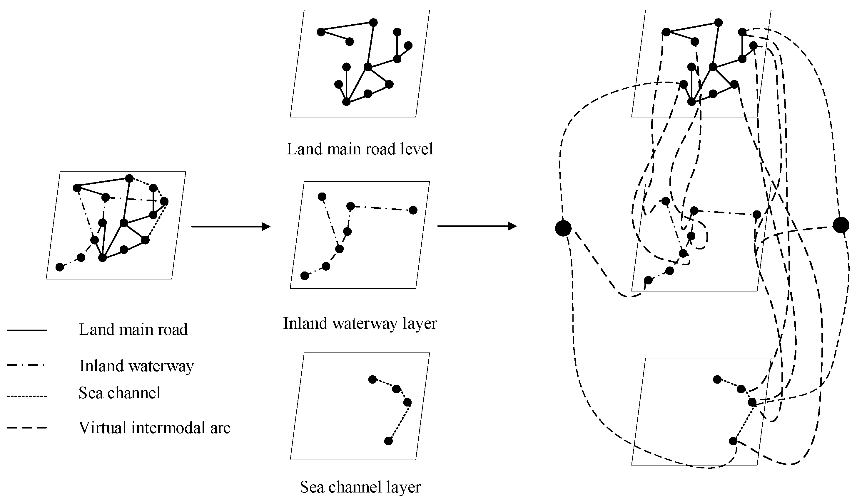
The roadway–water intermodal transport network examined in this study is a representative example of multimodal transport systems. It primarily consists of roadway transport subnetworks, inland waterway transport subnetworks, and maritime transport subnetworks, with transfer nodes that connect these three types of subnetworks. In constructing such a complex roadway–water intermodal transport network, it is first necessary to define and categorize the nodes and arcs within the network and to establish a unified topological representation. Specifically, as illustrated in Figure 1, actual roadway transport routes (e.g., expressways and national/provincial highways), inland waterway channels, and maritime shipping routes are abstracted as “transport arcs,” while physical facilities such as roadway transport hubs, toll stations, logistics parks, inland waterway ports, and coastal ports are abstracted as “nodes.” By connecting nodes via transport arcs, the roadway transport subnetwork, the inland waterway transport subnetwork, and the maritime transport subnetwork are constructed, respectively. On this basis, nodes that connect different transport subnetworks are defined as “transfer nodes,” and the edges linking transfer nodes to distinct transport subnetworks are termed “intermodal arcs,” representing the transshipment process of goods at these nodes.

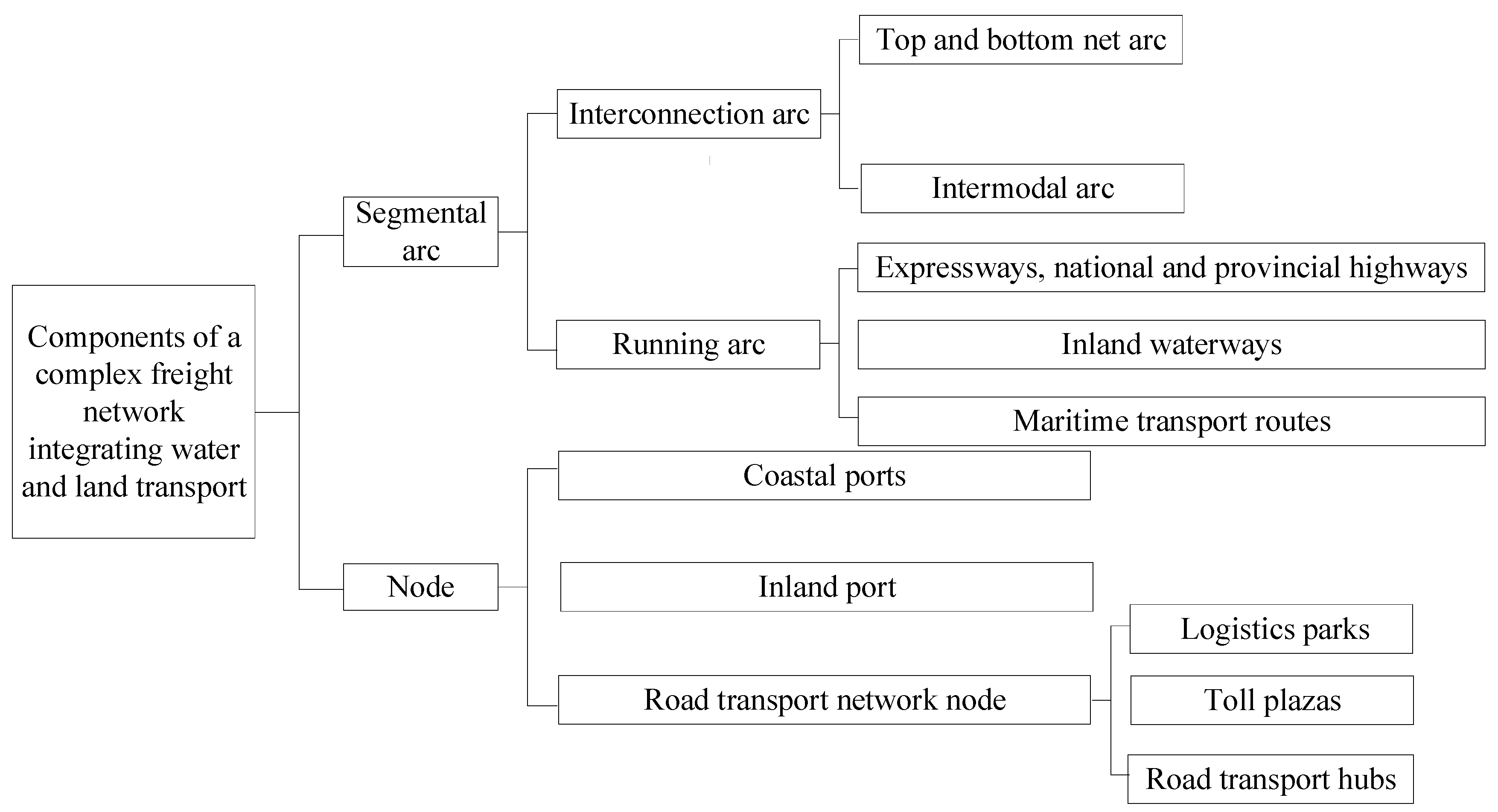
Figure 2 further specifies the constituent elements of each transport subnetwork. Specifically, the nodes of the roadway transport subnetwork include roadway transport hubs, toll stations, and logistics parks; the nodes of the inland waterway transport subnetwork are primarily inland waterway ports; and the nodes of the maritime transport subnetwork are primarily coastal ports. The edges of the roadway, inland waterway, and maritime transport subnetworks consist of expressways and national/provincial highways, inland waterway channels, and maritime shipping routes, respectively. These edges, represented by solid lines, are referred to as transport arcs. In contrast, the edges that connect different transport subnetworks via transfer nodes are represented by dashed lines and are referred to as intermodal arcs.

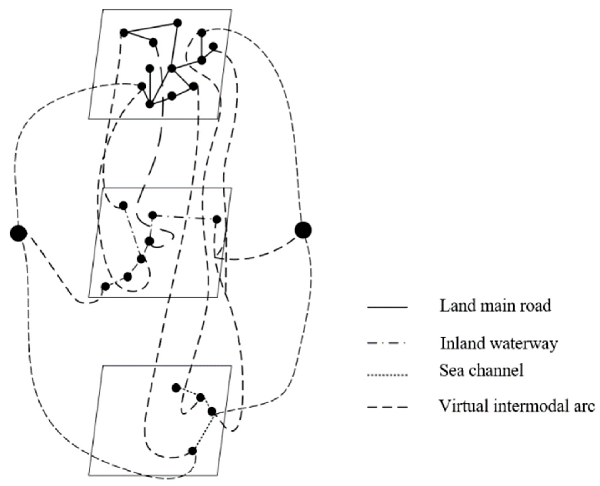
Figure 3 presents the constructed complex freight network integrating roadway and waterway systems, which is represented as a directed graph $G\left(N,A\right)$ with three layers. Here, $N$ denotes the set of nodes, including roadway nodes $N_{road}$, inland waterway nodes $N_{inland}$, maritime nodes $N_{maritime}$, and transfer nodes $N_{trans}$, i.e., $N=N_{road}\cup N_{inland}\cup N_{maritime}\cup N_{trans}$. Let $A$ denote the set of transport arcs, including roadway transport arcs $A_{road}$, inland waterway transport arcs $A_{inland}$, maritime transport arcs $A_{maritime}$, and intermodal arcs $A_{trans}$, i.e., $A=A_{road}\cup A_{inland}\cup A_{maritime}\cup A_{trans}$$.$

The network structure outlined above highlights the inherent constraints of the road–waterway intermodal system. First, transshipment nodes are obligatory points for inter-layer transfers, and their capacity imposes a hard constraint on network-wide modal conversion. Second, waterway subnetworks must connect to the roadway subnetwork through these nodes, meaning waterway transport cannot independently provide door-to-door service. Third, the roadway subnetwork exhibits the highest connectivity and can serve any origin–destination pair independently. This topological advantage fundamentally explains shippers’ default preference for road transport in the absence of policy intervention. These structural insights directly justify the choice of queuing models for impedance modeling, the inclusion of transshipment costs in the generalized cost function, and the independent consideration of transshipment subsidies in the subsidy strategy design.

3.2. Construction of Multimodal Traffic Impedance Models

Based on complex network theory, roadway, inland waterway, maritime, and transshipment nodes are integrated into a unified roadway–waterway bimodal freight network. This network explicitly defines the topological relationships among different modal subnetworks and the connectivity paths between nodes. However, the network structure alone cannot describe the actual transport time, cost, and carbon emissions incurred on links and at nodes. To compute the generalized transport cost of different routes for shippers, it is necessary to construct impedance functions for each type of transport link and transshipment node. Impedance serves as the foundation for flow assignment, and its accuracy directly determines the credibility of the subsequent freight flow diversion model. Therefore, building upon the complex freight network framework constructed above, this section establishes impedance models for roadway, inland waterway, maritime transport, and transshipment nodes, and integrates transport costs, time costs, carbon emission costs, and carbon subsidies into a unified generalized cost function, thereby achieving an effective coupling between network structure and operational costs.

3.2.1. Roadway Traffic Impedance Model

The roadway impedance function employs the classical BPR function to capture the nonlinear relationship between traffic flow and travel time. For a roadway arc $\left(i,j\right)$, the travel time is calculated as follows:

$$t_{ij}^{road}=t_{ij}^0\left[1+\alpha {\left({\displaystyle \frac{x_{ij}^{veh}}{Ca{p}_{ij}^{road}}}\right)}^{\beta }\right]$$

(1)

where $t_{ij}^0$ is the free-flow travel time on the roadway link $\left(i,j\right)$, $Ca{p}_{ij}^{road}$ is the capacity of the roadway link $\left(i,j\right)$, and $\alpha =0.15$ and $\beta =4$ are calibration parameters.

Roadway transport costs consist of freight costs, fuel costs, and tolls, which can be expressed as:

$$C_{ij}^{road}=\left({\displaystyle \frac{F{C}_{road}\cdot p_{fuel}\cdot f_{ij}^{road}}{100}}+p_{toll}\cdot f_{ij}^{road}+{\eta }_{road}\cdot Q_{ij}^{road}\right)\cdot L_{ij}^{road}$$

(2)

$$f_{ij}^{road}=\left[{\displaystyle \frac{Q_{ij}^{road}}{Loa{d}_{road}}}\right]$$

(3)

where $F{C}_{road}$ is the fuel consumption of roadway trucks, $p_{fuel}$ is the fuel price, $f_{ij}^{road}$ is the number of trips on the roadway link $\left(i,j\right)$, $p_{toll}$ is the roadway toll, ${\eta }_{road}$ is the unit freight transport price for roadway, $Q_{ij}^{road}$ is the freight volume on the roadway link $\left(i,j\right)$, and $L_{ij}^{road}$ is the transport distance on the roadway link $\left(i,j\right)$.

Carbon emissions from roadway transport are calculated based on fuel consumption:

$$E_{ij}^{road}={\displaystyle \frac{F{C}_{road}\cdot L_{ij}^{road}\cdot E{F}_{fuel}\cdot f_{ij}^{road}}{100}}$$

(4)

where $E{F}_{fuel}$ is the carbon emission factor.

Taking into account the influencing factors of transportation time, transportation costs, and carbon emission costs, the generalized cost of roadway transport is formulated as:

$$G{C}_{ij}^{road}=C_{ij}^{road}+V_{VOT}{t}_{ij}^{road}+p_{C{O}_2}{E}_{ij}^{road}$$

(5)

where $V_{VOT}$ is the value of the time coefficient, and $p_{C{O}_2}$ is the carbon price, taken as $p_{C{O}_2}=0.08$ CNY/kgCO₂ based on the China Carbon Market Price Report. This generalized cost function explicitly captures the effect of traffic congestion on roadway transport and serves as the foundation for freight flow assignment.

3.2.2. Inland Waterway Transport Impedance Model

Accurately calculating vessel waiting time at locks is central to the inland waterway transport impedance function. The total travel time on an inland waterway link consists of sailing time and lock waiting time. Sailing time is calculated using a time function:

$$t_{ij}^{sailing}={\displaystyle \frac{L_{ij}^{sailing}}{v^{inland}}}$$

(6)

where $L_{ij}^{sailing}$ denotes the sailing distance of vessels on the inland waterway link $\left(i,j\right)$ km, $v^{inland}$ denotes the sailing speed of vessels on inland waterways km/h.

Examining the entire lock passage process reveals that vessels inevitably experience queuing time. Hence, queuing theory is adopted to calculate the sojourn time. Assuming that the arrival rate $\lambda$ of inland waterway vessels at the lock follows a Poisson distribution and that the service rate $\mu$ of the lock follows an exponential distribution, the sojourn time of vessels at a single-chamber lock can be computed using an M/M/1 queuing system. The Poisson arrival and exponential service assumptions are simplifications adopted for mathematical tractability. In practice, vessel arrivals may be influenced by factors such as tides, weather, and lock scheduling rules. These assumptions are employed in this study to construct an analytically tractable queuing model, following the modeling conventions established in the lock congestion analysis literature, including Zheng et al. [9] and Mo et al. [8].

The lock system is stable when $\rho ={\displaystyle \frac{\lambda }{\mu }}<1$, based on the inland waterway traffic impedance model, the system stability of vessels passing through lock $k$ is calculated as follows:

$${\rho }_k={\displaystyle \frac{{\lambda }_k}{{\mu }_k}}$$

(7)

where ${\lambda }_k$ is the arrival rate of vessels at lock $k$, and ${\mu }_k$ is the lockage service rate of lock $k$. The vessel arrival rate is related to the link flow as follows:

$${\lambda }_k={\displaystyle \frac{x_{ij}^{inland}}{24Loa{d}_{inland}}}$$

(8)

where $x_{ij}^{inland}$ is the vessel flow on the inland waterway link $\left(i,j\right)$, and $Loa{d}_{inland}$ is the capacity tonnage of inland waterway vessels.

The average queue length of vessels at lock $k$ is:

$$L_{pk}={\displaystyle \frac{{\rho }_k^2}{1-{\rho }_k}}$$

(9)

The average waiting time in the queue is:

$$W_{pk}={\displaystyle \frac{{\rho }_k}{{\mu }_k\left(1-{\rho }_k\right)}}$$

(10)

The average total waiting time of vessels at the lock (including service time) is:

$$W_k^{inland}={\displaystyle \frac{1}{{\mu }_k\left(1-{\rho }_k\right)}}$$

(11)

For waterways with multiple locks, the total waiting time is the sum of the waiting times at each lock:

$$t^{inland}=t_{ij}^{sailing}+{\displaystyle \sum _{i=1}^n{W}_i}$$

(12)

where $n$ is the number of locks on the link $\left(i,j\right)$.

The transportation costs for inland waterway transport consist of freight costs, fuel costs, and lockage fees:

$$C_{ij}^{inland}={\displaystyle \frac{F{C}_{inland}\cdot p_{fuel}\cdot L_{ij}^{inland}\cdot f_{ij}^{inland}}{100}}+{\eta }_{water}\cdot L_{ij}^{inland}\cdot Q_{ij}^{inland}+n\cdot p_{lock}$$

(13)

$$f_{ij}^{inland}=\left[{\displaystyle \frac{Q_{ij}^{inland}}{Loa{d}_{inland}}}\right]$$

(14)

where $F{C}_{inland}$ is the fuel consumption of a 500-ton inland waterway vessel, $f_{ij}^{inland}$ is the number of freight trips on the inland waterway link $\left(i,j\right)$, ${\eta }_{water}$ is the unit transport price for waterway shipping. $Q_{ij}^{inland}$ is the total freight volume on the inland waterway link $\left(i,j\right)$, $p_{lock}$ is the lockage fee per vessel.

Carbon emissions for inland waterway transport consider only emissions generated during the navigation segment; emissions at locks are not taken into account:

$$E_{ij}^{inland}={\displaystyle \frac{F{C}_{inland}\cdot E{F}_{fuel}\cdot L_{ij}^{inland}\cdot f_{ij}^{inland}}{100}}$$

(15)

In addition to the generalized costs of roadway transport, lockage fees for vessels are also considered. Therefore, the generalized cost for inland waterway transport (excluding the generalized cost at transshipment nodes) is:

$$G{C}_{ij}^{inland}=C_{ij}^{inland}+V_{VOT}{t}_{in}^{inland}+p_{C{O}_2}{E}_{ij}^{inland}-S_{ij}^{inland}$$

(16)

where $S_{ij}^{inland}$ is the subsidy expenditure on the inland waterway link $\left(i,j\right)$.

The M/M/1 model enables an accurate analysis of the impact of vessel flow on lock waiting time, which facilitates the design of different subsidy schemes within the generalized cost function for inland waterway transport and provides a theoretical basis for government decision-making.

3.2.3. Maritime Transport Impedance Model

Maritime transport is characterized by large capacity, low cost, and low carbon emissions. However, its transit time is relatively fixed due to weather conditions and shipping schedules. Moreover, since maritime transport is free from the complex traffic disturbances encountered in roadway and inland waterway transport, its travel time can be directly computed using a fixed-time model. The computation of maritime transport cost is similar to that of inland waterway transport cost. However, since maritime transport is not subject to lock constraints, the maritime transport cost excludes the lockage fee, i.e.,

$$C_{ij}^{maritime}={\displaystyle \frac{F{C}_{maritime}\cdot p_{fuel}\cdot L_{ij}^{maritime}\cdot f_{ij}^{maritime}}{100}}+{\eta }_{water}\cdot L_{ij}^{maritime}\cdot Q_{ij}^{maritime}$$

(17)

$$f_{ij}^{maritime}=\left[{\displaystyle \frac{Q_{ij}^{maritime}}{Loa{d}_{maritime}}}\right]$$

(18)

where $f_{ij}^{maritime}$ is the number of freight trips on the maritime link $\left(i,j\right)$, $Q_{ij}^{maritime}$ is the total freight volume on the maritime link $\left(i,j\right)$, $Loa{d}_{maritime}$ is the capacity tonnage of maritime vessels, and $F{C}_{maritime}$ is the fuel consumption of a 1500-t maritime vessel.

The calculation of carbon emissions for maritime transport primarily includes emissions generated during the maritime transport segment:

$$E_{ij}^{maritime}={\displaystyle \frac{F{C}_{maritime}\cdot E{F}_{fuel}\cdot L_{ij}^{maritime}\cdot f_{ij}^{maritime}}{100}}$$

(19)

The generalized cost of maritime transport (excluding the generalized cost at transshipment nodes) is:

$$G{C}_{ij}^{maritime}=C_{ij}^{maritime}+V_{VOT}{t}_{in}^{maritime}+p_{C{O}_2}{E}_{ij}^{maritime}-S_{ij}^{maritime}$$

(20)

where $S_{ij}^{maritime}$ is the subsidy expenditure on the maritime link $\left(i,j\right)$.

3.2.4. Transshipment Node Impedance Model

The transshipment node is a critical link in the freight transfer process, and its operational efficiency directly affects the efficiency of the entire transport chain. By analyzing the complete process from freight arrival to departure at a transshipment node, it can be observed that multiple handling facilities typically operate simultaneously at the node. However, since freight arrives at the transshipment node concurrently, a queuing time arises during the waiting process for handling. Therefore, a queuing model is required to investigate the transfer time of freight at the transshipment node. It is assumed that the arrival rate of freight at the transshipment node, $\lambda$, follows a Poisson distribution; the service rate of each handling facility, $\mu$, follows an exponential distribution; and the transshipment node is equipped with $c$ parallel handling facilities. Accordingly, an M/M/c queuing model is constructed to study the transfer time of freight at the transshipment node.

In the M/M/c queuing model, the stability condition is given by: $\rho ={\displaystyle \frac{\lambda }{c\mu }}$, The probability that no freight is being handled at the transshipment node $m$ is:

$$P_{m0}={\left[{\displaystyle \sum _{n=0}^{c_m}\frac{{\left(c_m{\rho }_m\right)}^n}{n!}}+{\displaystyle \frac{{\left(c_m{\rho }_m\right)}^{c_m}}{c_m!\left(1-{\rho }_m\right)}}\right]}^{-1}$$

(21)

Based on the probability of zero cargo in the system, several other performance metrics can be derived. The average queue length (number of cargo units waiting in the queue) is:

$$L_m={\displaystyle \frac{{\left(c_m{\rho }_m\right)}^{c_m}{\rho }_m}{c_m!{(1-{\rho }_m)}^2}}{P}_{m0}$$

(22)

The average waiting time in the queue is:

$$W_{pm}={\displaystyle \frac{L_m}{{\lambda }_m}}$$

(23)

The average sojourn time of freight at the transshipment node $m$ is:

$$t_m^{trans}=W_{pm}+{\displaystyle \frac{1}{{\mu }_m}}$$

(24)

Transshipment costs primarily consist of two components: storage fees and handling fees. Storage fees are calculated based on cargo weight and dwell time at the port, while handling fees are calculated based on the volume of cargo handled:

$$C_m^{trans}=\left({\vartheta }_{store}\cdot t_m^{trans}+p_{handle}\right)\cdot Q_{ij}^m$$

(25)

where ${\vartheta }_{store}$ is the storage cost per unit weight per unit time, $p_{handle}$ is the handling cost per unit weight, and $Q_{ij}^m$ is the transshipment freight volume at transshipment node $m$ on link $\left(i,j\right)$.

Carbon emissions at transshipment nodes primarily arise from fuel consumption by handling equipment during the loading and unloading process:

$$E_m^{trans}=c\cdot F{C}_{trans}\cdot E{F}_{fuel}\cdot t_m^{trans}$$

(26)

Carbon subsidies for transshipment nodes are calculated based on the volume of cargo transferred. Therefore, the generalized cost at a transshipment node is:

$$G{C}_m^{trans}=C_m^{trans}+V_{VOT}{t}_m^{trans}+p_{C{O}_2}{E}_m^{trans}-S_m^{trans}$$

(27)

where $S_m^{trans}$ is the subsidy amount at the transshipment node $m$.

By integrating the impedance functions of the various transport modes described above, and considering that shippers, when choosing a transport route, need to comprehensively account for transport costs, time costs, carbon emission costs, and carbon subsidies, a generalized cost function is formulated. For a complete intermodal transport route $\left(i,j\right)$, the generalized cost is expressed as:

$$G{C}_{ij}={\displaystyle \sum _{a\in A_{road}}G{C}_a^{road}}+{\displaystyle \sum _{a\in A_{inland}}G{C}_a^{inland}}+{\displaystyle \sum _{a\in A_{maritime}}G{C}_a^{maritime}}+{\displaystyle \sum _{m\in N_{trans}}G{C}_m^{trans}}$$

(28)

The impedance model constructed in this study is established under given topological structures and infrastructure capacities of the road–waterway bimodal network. Parameters such as inland waterway channel grades, lock throughput capacities, and port handling efficiencies are calibrated based on current empirical data, reflecting the actual supply conditions of the waterway network in the study region. The mechanism of carbon subsidies operates precisely within these established network constraints: by reducing the generalized cost of waterway transport segments, subsidies guide shippers to reassess and choose among existing roadway, inland waterway, and maritime routes, rather than altering the network structure itself. Consequently, the optimization of subsidy strategies is inherently constrained by factors such as channel throughput capacity, lock service rates, and port handling capacities. When subsidies reach a certain level, the capacity of the waterway network tends toward saturation, and further increases in subsidies can no longer produce additional freight flow diversion.

4. Bi-Level Programming Model for Freight Flow Assignment and Subsidy Optimization on Roadway–Waterway Bimodal Networks and Its Algorithm Design

4.1. Problem Description

In the road–waterway bimodal freight system, roadway transport carries the vast majority of medium- and long-distance freight demand, and its high carbon emission intensity constitutes a major source of regional transport emissions to be mitigated. To optimize the freight structure and reduce system-wide carbon emissions, the government can guide a portion of freight from roadway to waterway through differentiated carbon subsidy policies. However, realizing this process entails two interrelated core issues: first, the subsidy strategy design problem, i.e., how to formulate an optimal subsidy scheme that simultaneously accounts for fiscal efficiency and emission reduction targets; second, the freight flow diversion pattern problem, i.e., how the freight flow distribution will change under the subsidy incentive. These two issues are mutually prerequisite and restrictive, constituting the dual analytical focus of this study.

In this study, the government acts as the upper-level decision maker, aiming to minimize carbon emissions and subsidy expenditure, and determines the subsidy rates for inland waterway, maritime, and transshipment nodes. Shippers, as lower-level followers, choose freight routes based on the criterion of minimizing the generalized transport cost. Government subsidies influence shippers’ choices by altering the relative costs on waterway links, while the resulting equilibrium flow distribution serves as a feedback signal to inform subsequent subsidy decisions. A bi-level programming model is constructed to describe this interactive process, under the following basic assumptions: shippers are perfectly rational and have complete information; a unique user equilibrium state exists; carbon emission costs are calculated at a fixed carbon price; carbon subsidies are only applicable to waterway transport and transshipment activities; the network structure is static and known; freight is considered as homogeneous bulk cargo; and transshipment occurs only at designated nodes and at most once per route.

4.2. Carbon Subsidy Design

As an economic incentive instrument directly targeting waterway transport costs, carbon subsidies aim to provide financial support for low-carbon transport modes, compensate for the additional cost burdens of waterway transport, and restructure the relative cost advantages among different modes, thereby guiding shippers to prioritize low-carbon transport options. In the road–waterway bimodal freight system, the effect of carbon subsidies is more immediate, primarily manifested in the adjustment of the generalized transport cost.

Considering that transport distance and freight turnover are readily observable and verifiable, it is more straightforward to calculate subsidies based on freight volume. According to the subsidy recipients, carbon subsidies are classified into three categories: inland waterway transport subsidies, maritime transport subsidies, and transshipment node subsidies.

Inland waterway transport subsidies are provided for freight transported via inland waterways, calculated as:

$$S_{ij}^{inland}=s_{ij}^{inland}\cdot L_{ij}^{inland}\cdot Q_{ij}^{inland}$$

(29)

where $S_{ij}^{inland}$ denotes the amount of inland waterway carbon subsidy, and $s_{ij}^{inland}$ is the subsidy rate for inland waterway transport (CNY/t·km).

Inland waterway transport suffers from relatively low sailing speeds, limited lock throughput capacity, and low waterway grades, which result in high transit time costs and additional lockage fees. Accordingly, the primary role of inland waterway transport subsidies is to compensate for these disadvantages in time and lockage costs, incentivize shippers to opt for inland waterway transport, and provide policy support for the upgrading and improvement of inland waterway infrastructure, thereby facilitating the continuous enhancement of inland navigation capacity.

Maritime transport subsidies are granted to freight transported via maritime routes, and are calculated as follows:

$$S_{ij}^{maritime}=s_{ij}^{maritime}\cdot L_{ij}^{maritime}\cdot Q_{ij}^{maritime}$$

(30)

where $S_{ij}^{maritime}$ denotes the amount of maritime carbon subsidy, and $s_{ij}^{maritime}$ is the subsidy rate for maritime transport (CNY/t·km). Maritime transport features advantages such as large capacity, low unit carbon emissions, and well-established shipping routes, but it is constrained by the efficiency of port collection and distribution systems. The purpose of maritime transport subsidies is to guide the diversion of bulk freight from roadway to maritime transport, alleviate the pressure on roadway transport, optimize the port collection and distribution structure, and promote the improvement and development of maritime shipping networks.

Transshipment node subsidies are primarily applicable to port nodes where a modal shift occurs, such as roadway-to-inland waterway, inland waterway-to-maritime, and roadway-to-maritime. This requires that a modal shift must occur at the port node eligible for transshipment subsidies; single-mode transport operations are not covered by the subsidy scheme. Since distance is not considered as an influencing factor in the transshipment process at these nodes, the transshipment node subsidy is calculated as follows:

$$S_m^{trans}=s_m^{trans}{Q}_m$$

(31)

where $s_m^{trans}$ is the transshipment subsidy rate (CNY/t), and $Q_m$ is the freight flow at the transshipment node $m$. This subsidy aims to reduce the intermodal transfer costs between different transport modes, compensate for the time delays and handling charges incurred during the transshipment process, and enhance the overall efficiency of intermodal transport.

In summary, the total subsidy obtained on a given route consists of three components:

$$S_{ij}^{total}={\displaystyle \sum _{l\in A_{inland}}{S}_l^{inland}\cdot {\varsigma }_{lij}}+{\displaystyle \sum _{l\in A_{maritime}}{S}_l^{maritime}\cdot {\varsigma }_{lij}}+{\displaystyle \sum _{n\in N_{trans}}{S}_n^{trans}\cdot {\tau }_{nij}}$$

(32)

where ${\varsigma }_{lij}$ equals 1 if link $l$ is an inland waterway/maritime link on route $\left(i,j\right)$, and 0 otherwise; ${\tau }_{nij}$ equals 1 if a modal shift occurs at node $n$ on route $\left(i,j\right)$, and 0 otherwise.

This formula explicitly captures the cumulative structure of carbon subsidies along an intermodal route, providing a direct basis for modeling shippers’ route choice behavior in the lower level of the subsequent bi-level programming model.

4.3. Lower-Level Model: Freight Flow Allocation Model

The objective function of the lower-level model is to minimize the generalized transport cost of the entire road–waterway freight system, i.e., shippers pursue the minimization of the comprehensive transport cost under the guidance of carbon subsidy policies. The generalized transport cost consists of three components: direct transport cost, transshipment cost, and time window penalty cost. The model includes three main decision variables: $x_{ij}^r$ denotes the freight volume (in tons) on transport arc $\left(i,j\right)$ using mode $r$ (roadway, inland waterway, or maritime, $Y=\left\{road,inland,maritime\right\}$), which is a continuous variable subject to arc capacity constraints; $y_m$ denotes the cargo transshipment volume (in tons) at transshipment node $m$, which is a continuous variable subject to node transshipment capacity constraints; and $z_{ij}^l$ is a binary variable indicating whether origin–destination pair $\left(i,j\right)$ selects feasible path $l$ (1 if selected, 0 otherwise). The objective function of the lower-level model is:

$$\begin{array}{l}\min Z_{lower}={\displaystyle \sum _{ij}{\displaystyle \sum _{r\in Y}\left[C_{ij}^Y+V_{VOT}{t}_{ij}^Y+p_{C{O}_2}{E}_{ij}^Y-\theta S_{ij}^{total}\right]\cdot x_{ij}^r}}+{\displaystyle \sum _m\left[C_{ij}^{trans}+V_{VOT}{t}_{ij}^{trans}+p_{C{O}_2}{E}_{ij}^{trans}-S_{ij}^{trans}\right]\cdot y_m}+\\ +{\displaystyle \sum _{ij}{\displaystyle \sum _{l}M\cdot \max \left(0,t_{ij}^l-t_{ij}^{latest}\right)}}\end{array}$$

(33)

The meaning and composition of each term are as follows: The first term, ${\displaystyle \sum _{ij}{\displaystyle \sum _{r\in Y}\left[C_{ij}^Y+V_{VOT}{t}_{ij}^Y+p_{C{O}_2}{E}_{ij}^Y-\theta S_{ij}^{total}\right]\cdot x_{ij}^r}}$, represents the direct transport cost, which comprises freight transport charges, fuel costs, time costs, road tolls, lockage fees, and other direct expenses. $\theta$ denotes the subsidy effectiveness coefficient, taken as 0.9 in the computational study. The subsidy reduces the direct cost of waterway transport, thereby enhancing its competitiveness. The second term, ${\displaystyle \sum _m\left[C_{ij}^{trans}+V_{VOT}{t}_{ij}^{trans}+p_{C{O}_2}{E}_{ij}^{trans}-S_{ij}^{trans}\right]\cdot y_m}$, captures the transshipment cost, which includes the handling cost, transshipment time, carbon emissions generated during the transshipment process, and the carbon subsidy at the transshipment node. The third term, ${\displaystyle \sum _{ij}{\displaystyle \sum _{l}M\cdot \max \left(0,t_{ij}^l-t_{ij}^{latest}\right)}}$, is the time window penalty function, which reflects the timeliness requirements of freight transport. When the total travel time on route $l$ exceeds the latest permissible delivery time on that route, a penalty is imposed. $M$ is the time window penalty coefficient, typically assigned an arbitrarily large value to discourage tardiness; in this study, $M={10}^{10}$. This mechanism ensures that the model prioritizes transport routes meeting the timeliness constraints during the optimization process and precludes the adoption of infeasible solutions.

In summary, while minimizing the generalized transport cost, the lower-level objective function comprehensively balances economic costs, time constraints, carbon emission impacts, and policy incentives, thereby providing an optimization criterion that aligns with shippers’ rational choice behavior in freight flow assignment.

s.t

$${\displaystyle \sum _m{x}_{ij}^r}=D_{ij} \forall i,j$$

(34)

$${\displaystyle \sum _{m\in N_{trans}}{z}_{ij}^l}\le 1 \forall i,j,l$$

(35)

$$y_m\le Q_m^{\max } \forall m\in N^{trans} w_{inland}\le W_a \forall a\in A_{inland}$$

(36)

$$y_m={\displaystyle \sum _{ij}{\displaystyle \sum _r{z}_{ij}^l\cdot x_{ij}^{r,road}}}$$

(37)

$$x_{ij}^r\ge 0, y_m\ge 0, z_{ij}^l\in \left\{0,1\right\}$$

(38)

where $Q_m^{\max }$ is the maximum handling capacity of the transshipment node $m$, $w_{inland}$ is the standard capacity tonnage of inland waterway vessels, and $W_a$ denotes the maximum navigable tonnage on link $a$. Constraints (34)–(38) represent flow conservation constraints, route uniqueness constraints, transshipment node capacity constraint and, vessel tonnage–waterway navigability compatibility constraints, flow consistency constraints, and non-negativity constraints, respectively.

4.4. Upper-Level Model: Differentiated Subsidy Decision Model

The upper-level government subsidy decision model adopts a bi-objective optimization approach, aiming to simultaneously minimize carbon emissions and minimize government subsidy expenditure. These two objectives inherently conflict with and counterbalance each other, necessitating a trade-off during the optimization process. The differentiated subsidy decision model involves three decision variables: $s=\left(s_{inland},s_{maritime},s_{trans}\right)$; the carbon subsidy standard for inland waterway transport is: $s_{inland}\in \left[0,s_{inland}^{\max }\right]$, where $s_{inland}^{\max }\in \left[0,0.25\right]$ CNY/t·km. The carbon subsidy standard for maritime transport is: $s_{maritime}\in \left[0,s_{maritime}^{\max }\right]$, where $s_{maritime}^{\max }\in \left[0,0.28\right]$ CNY/t·km.

The carbon subsidy standard for transshipment nodes is: $s_{trans}\in \left[0,s_{trans}^{\max }\right]$, where $s_{inland}^{\max }\in \left[0,20\right]$. These three variables are independent of one another, allowing the government to implement targeted carbon subsidies. The first objective function is to minimize total carbon emissions:

$$\min Z_1\left(s\right)={\displaystyle \sum _{ij}{\displaystyle \sum _r{E}_{ij}^r\cdot x_{ij}^r\left(s\right)}}+{\displaystyle \sum _m{E}_m^{trans}\cdot y_m\left(s\right)}$$

(39)

where ${\displaystyle \sum _{ij}{\displaystyle \sum _r{E}_{ij}^r\cdot x_{ij}^r\left(s\right)}}$ represents the total transport carbon emissions, which is the sum of carbon emissions from inland waterway, roadway, and maritime transport. Based on calculations, the unit carbon emission of roadway transport is 0.2 kgCO₂/t·km, that of maritime transport is 0.015 kgCO₂/t·km, and that of inland waterway transport is 0.03 kgCO₂/t·km. A comparison of carbon emission intensities reveals that roadway transport exhibits the highest carbon emission intensity, approximately 6.7 times that of inland waterway transport and 13.3 times that of maritime transport. Therefore, guiding freight flow from roadway to waterway transport through carbon subsidy policies can substantially reduce the carbon emission level of the entire transport system, yielding significant carbon reduction benefits.

The second objective function is to minimize the total government subsidy expenditure, expressed as:

$$\min Z_2\left(s\right)=s_{inland}{\displaystyle \sum _{l\in A_{inland}}{L}_l\cdot x_l^{*}\left(s\right)}+s_{maritime}{\displaystyle \sum _{l\in A_{maritime}}{L}_l\cdot x_l^{*}\left(s\right)}+s_{trans}{\displaystyle \sum _{m\in N_{trans}}{y}_m^{*}\left(s\right)}$$

(40)

where the first term, $s_{inland}{\displaystyle \sum _{l\in A_{inland}}{L}_l\cdot x_l^{*}\left(s\right)}$, is the total inland waterway subsidy expenditure, with $L_l$ denoting the inland waterway transport distance on link $l$, and $x_l^{*}\left(s\right)$ denoting the equilibrium freight flow on link $l$ obtained from the lower-level model under the given subsidy scheme. The second term, $s_{maritime}{\displaystyle \sum _{l\in A_{maritime}}{L}_l\cdot x_l^{*}\left(s\right)}$, is the total maritime subsidy expenditure, where $L_l$ denotes the maritime transport distance on link $l$, and $x_l^{*}\left(s\right)$ is the equilibrium freight flow on link $l$ derived from the lower-level model. The third term, $s_{trans}{\displaystyle \sum _{m\in N_{trans}}{y}_m^{*}\left(s\right)}$, is the total transshipment node subsidy expenditure, with $y_m^{*}\left(s\right)$ representing the equilibrium transshipment freight volume at the node $m$ obtained from the lower-level model under the given subsidy scheme.

s.t

$$s_{inland}{\displaystyle \sum _{l\in A_{inland}}{L}_l\cdot x_l^{*}}+s_{maritime}{\displaystyle \sum _{l\in A_{maritime}}{L}_l\cdot x_l^{*}}+s_{trans}{\displaystyle \sum _{m\in N_{trans}}{y}_m^{*}\le B}$$

(41)

where $B$ denotes the upper limit of government carbon subsidy expenditure.

$$0\le s_{inland}\le s_{inland}^{\max }, 0\le s_{maritime}\le s_{maritime}^{\max }, 0\le s_{trans}\le s_{trans}^{\max }$$

(42)

The set of constraints consists of the fiscal budget constraint (41) and the upper and lower bounds on the subsidy standards (42).

4.5. Solution Algorithm

The upper-level model in this paper is a two-objective optimization problem with conflicting objectives. The NSGA-II algorithm is employed to solve this problem, and its performance is compared with that of the NSGA and NSGA-III algorithms. The steps of the NSGA-II algorithm are as follows:

• An initial population is generated using real-number encoding, where each chromosome represents a subsidy scheme.
• For each individual, the lower-level model is solved using the Method of Successive Averages (MSA) to determine the user equilibrium. The total carbon emissions and total subsidy expenditure across all routes are then calculated as the fitness values.
• A fast non-dominated sorting procedure is performed to stratify the population individuals based on Pareto dominance relationships.
• The crowding distance of individuals within the same non-dominated front is calculated, with the distance of boundary individuals set to infinity.
• An offspring population is generated using tournament selection, simulated binary crossover (SBX), and polynomial mutation.
• The parent and offspring populations are merged, and the next-generation population is selected using an elite retention strategy.
• Steps 2–6 are repeated until the maximum number of evolutionary generations is reached or the convergence criteria are met.

5. Case Study

5.1. Case Background and Data

The freight OD data used in this study were obtained from a dedicated traffic survey conducted in the Cixi–Yuyao region in 2020. Ten key cross-sections were selected for the survey, including toll stations along the G15 Shenyang–Haikou Expressway, the G329 National Highway, and the Shenglu Elevated Road. A combination of roadside interviews and license plate recognition was adopted to conduct continuous 16-h OD surveys (6:00–22:00) and 24-h traffic volume observations. Information on vehicle type, loading capacity, freight category, origin, destination, and travel route was recorded, yielding approximately 12,000 valid samples. After expanding the samples to daily traffic volumes using hourly traffic counts as control totals, the OD matrix was iteratively calibrated using the capacity-restraint method: with observed traffic volumes at each cross-section serving as the control targets, OD pair values were proportionally adjusted whenever the deviation between simulated and observed volumes exceeded 15%, until the error converged to within 15% at all cross-sections. The resulting OD matrix, expressed in tons/day as shown in

Table 1. Origin–Destination matrix for outbound shipments from the Cixi area.

OD	Origin	Destination	Freight Volume (Tons/Year)	Freight Volume (Tons/Day)
OD1	CX	BL	1,721,470	5215
OD2	CX	ZH	171,000	518
OD3	CX	FH	120,000	364
OD4	CX	SH	186,100	564
OD5	CX	YY	128,767	390
OD6	CX	JD	120,100	364
OD7	CX	CS	86,000	261
OD8	CX	XS	54,133	164
OD9	CX	WL	42,767	130
OD10	CX	LQ	34,100	103
OD11	CX	XA	34,100	103
Total	—	—	2,698,537	8176

and

Table 2. Origin–Destination matrix for inbound freight flows in the Cixi area.

OD	Origin	Destination	Freight Volume (Tons/Year)	Freight Volume (Tons/Day)
OD12	YY	CX	1,887,940	5721
OD13	ZH	CX	620,667	1881
OD14	BL	CX	706,134	2140
OD15	YZ	CX	280,333	849
OD16	SH	CX	47,500	144
OD17	GS	CX	66,500	202
OD18	FH	CX	58,000	176
OD19	HS	CX	7000	21
OD20	JD	CX	34,333	104
Total	-	-	3,708,407	11,238

, covers 20 major OD pairs with an average daily total freight volume of approximately 19,400 tons, thereby providing the data foundation for subsequent network flow assignment and the empirical analysis of subsidy strategies.

5.2. Design of Subsidy Expenditure Caps and Algorithm Parameter Settings

Based on the estimated theoretical maximum subsidy requirement (approximately CNY 876,000/day) and the characteristics of the marginal abatement cost curve, three subsidy expenditure caps are established: low (CNY 120,000/day), medium (CNY 350,000/day), and high (CNY 700,000/day). The low cap corresponds to the initial stage, where marginal emission reduction efficiency is the highest; the medium cap marks the critical inflection point of marginal efficiency, with CNY 350,000/day identified as the subsidy efficiency frontier; and the high cap corresponds to the saturation stage and serves to verify the marginal failure of excessive subsidies. Together, these three levels encompass the full policy spectrum from tight fiscal constraints to high expenditure, providing an analytical basis for comparing the emission reduction effectiveness and fiscal efficiency under different subsidy intensities.

The NSGA, NSGA-II, and NSGA-III algorithms all adopt identical basic parameters: population size $N=100$, maximum number of generations $G=200$, crossover probability $p_c=0.9$, mutation probability $p_m=0.33$, crossover distribution index ${\kappa }_c=20$, and mutation distribution index ${\psi }_m=20$. These parameters were determined based on prior experience and preliminary experimental results. For the NSGA-specific parameter, the sharing radius ${\sigma }_{share}$ is set to 0.1, a value that has been shown through multiple trials to maintain population diversity effectively. The NSGA-II algorithm adopts tournament selection with a tournament size of 2, with distribution indices of 15 and 20 for the crossover and mutation processes, respectively. For the NSGA-III algorithm, reference points are generated using the Das–Dennis method; given the bi-objective nature of the optimization problem, the number of reference points is set to 100, matching the population size. All three algorithms adopt the same encoding scheme. To mitigate the effect of randomness, each algorithm is independently executed 20 times, and the average results are taken as the final outcomes for comparative analysis.

5.3. Analysis of Results

(1)

No-subsidy benchmark scenario

In the absence of subsidies, as shown in

Table 3. Changes in OD freight distribution without subsidies.

OD	Origin	Destination	Roadway Share (%)	Waterway Share (%)
OD1	CX	BL	99.20%	0.80%
OD2	CX	ZH	99.85%	0.15%
OD3	CX	FH	100.00%	0.00%
OD4	CX	SH	89.06%	10.94%
OD5	CX	YY	100.00%	0.00%
OD6	CX	JD	93.79%	6.21%
OD7	CX	CS	69.45%	30.55%
OD8	CX	XS	99.98%	0.02%
OD9	CX	WL	100.00%	0.00%
OD10	CX	LQ	100.00%	0.00%
OD11	CX	XA	100.00%	0.00%
OD12	YY	CX	100.00%	0.00%
OD13	ZH	CX	99.96%	0.04%
OD14	BL	CX	99.80%	0.20%
OD15	YZ	CX	100.00%	0.00%
OD16	SH	CX	89.06%	10.94%
OD17	GS	CX	99.98%	0.02%
OD18	FH	CX	100.00%	0.00%
OD19	HS	CX	100.00%	0.00%
OD20	JD	CX	93.79%	6.21%

, the system-wide waterway transport share was merely 1.74%, and 12 out of the 20 OD pairs exhibited zero waterway share, with roadway bearing almost the entire freight volume. The traffic load on critical segments such as G329 and the G15 Shenyang–Haikou Expressway reached 0.78–0.79, indicating chronic congestion, and shippers had no incentive to spontaneously shift to waterway.

(2)

Comparison of subsidy effects

Table 4. Optimal emission reduction outcomes under different subsidy levels: a comparison.

Subsidy Expenditure Level	Minimum Carbon Emissions (Tons CO2/Day)	Emission Reduction (Tons/Day)	Reduction Rate	Waterway Share	Marginal Abatement Cost (CNY/t CO2)
No subsidy	220.72	–	–	1.74%	–
Low budget	197.51	23.21	10.5%	14.00%	5170
Medium budget	187.45	33.27	15.1%	22.7%	2231
High budget	187.45	33.27	15.1%	22.7%	–

summarizes the optimal emission reduction outcomes under the three subsidy expenditure caps. Under the low cap (CNY 120,000/day), the waterway share rose to 14.00%, carbon emissions decreased from 220.72 tons/day to 197.51 tons/day, yielding a reduction of 23.21 tons/day (a reduction rate of 10.5%). Under the medium cap (CNY 350,000/day), the waterway share reached 22.70%, carbon emissions dropped to 187.45 tons/day, and the cumulative reduction amounted to 33.27 tons/day (a reduction rate of 15.1%), with all three subsidy standards attaining their maximum values. Under the high cap (CNY 700,000/day), neither the waterway share nor carbon emissions changed further, and the marginal diversion efficiency approached zero. In summary, the efficiency frontier for carbon subsidy policies in the Ciyu region is approximately CNY 350,000/day. Subsidies should be focused on medium- and long-haul routes, while short-haul freight transport needs to be optimized in conjunction with other modes.

(3)

Evolutionary Pattern of Differentiated Subsidy Strategies

As shown in

Table 5. Evolution of differentiated subsidy strategies across budget phases.

Budget Stage	Subsidy Expenditure Range	Subsidy Focus	Inland Waterway Subsidy Rate	Maritime Subsidy Rate	Transshipment Subsidy Rate	Waterway Share
Initial stage	0-CNY 120,000/ day	Prioritizing maritime transport, supplemented by transshipment	0	0.05–0.18 CNY/t·km	0–20 CNY/t	1.74% → 14.0%
Intermediate stage	CNY 120,000–350,000/day	Equal emphasis on inland waterway and maritime transport	0 → 0.25	0.18 → 0.28	20	14.0% → 22.7%
Saturation stage	>CNY 350,000/day	Freeze rate, prioritize efficiency	0.25	0.28	20	22.7%

, the subsidy strategy exhibits a three-stage evolutionary pattern. In the initial stage (0–CNY 120,000/day), maritime subsidies were prioritized and supplemented by transshipment subsidies, while inland waterway subsidies remained zero. The waterway share increased from 1.74% to 14.00%, with a reduction of 23.21 tons CO₂/day. This indicates that in the early phase, priority should be given to subsidizing transshipment nodes and maritime transport to unlock the potential of medium- and long-distance waterway transport at a relatively low cost, while inland waterway subsidies are temporarily withheld due to their low efficiency resulting from lock bottlenecks.

In the intermediate stage (CNY 120,000–350,000/day), equal emphasis was placed on inland waterway and maritime subsidies, with transshipment subsidies stabilizing at CNY 20/t. The waterway shares further rose to 22.70%, and cumulative emission reductions reached 33.27 tons CO₂/day. During this stage, the introduction of inland waterway subsidies enabled some short-haul freight, such as OD1, to be diverted via inland waterways, reducing the load on the G15 Shenyang–Haikou Expressway to below 0.55. The policy focus shifted from solely maritime subsidies to a balanced approach between inland waterway and maritime subsidies, with the subsidy ratio gradually adjusting from 1.5 to below 1.0.

In the saturation stage (subsidy > CNY 350,000/day), the subsidy levels stabilized, and neither the waterway share nor carbon emissions exhibited further changes. This stabilization occurred because lock throughput and port handling capacities had reached their limits, causing vessel queuing times to rise sharply and capping the daily waterway freight volume at approximately 4400 tons. Consequently, the policy focus should shift toward expanding inland waterway capacity and upgrading port facilities.

5.4. Algorithm Performance Comparison

To address the differentiated subsidy optimization problem for road–waterway intermodal transport, the NSGA, NSGA-II, and NSGA-III algorithms were employed, and their performances exhibited notable differences. The three algorithms were evaluated in terms of the inverted generational distance (IGD), hypervolume (HV), convergence, computation time. The results, as shown in

Table 6. Comparison of Performance Among the NSGA, NSGA-II, and NSGA-III Algorithms.

Metric	NSGA	NSGA-II	NSGA-III
IGD	0.0150	0.0041	0.0065
HV	0.650	0.887	0.870
Convergence (generations)	186	123	90
Computation time (s)	700	742	1112

, indicate that overall, the NSGA-II algorithm delivered the best performance. Its IGD value was 0.0041, markedly lower than that of NSGA (0.015) and NSGA-III (0.0065), indicating that the solution set obtained by NSGA-II lies closer to the true Pareto front. In terms of solution diversity, the HV of NSGA-II reached 0.887, higher than that of NSGA (0.650) and NSGA-III (0.870), suggesting that its solution set covers a wider range and achieves superior diversity. Regarding computational efficiency, although NSGA-III exhibited the fastest convergence (90 generations), it required the longest computation time (1112 s), averaging approximately 12.4 s per generation, which results in excessively high computational cost. The NSGA algorithm required the shortest computation time (700 s) but performed the worst in both convergence and diversity. In contrast, NSGA-II converged in 123 generations with a computation time of 742 s, averaging about 6.0 s per generation, thus striking the best balance between convergence speed and per-generation computational cost and achieving the highest overall computational efficiency. In summary, the NSGA-II algorithm outperforms the other two algorithms in terms of solution convergence, diversity, and overall performance, making it the most suitable algorithm for solving the proposed model.

5.5. Sensitivity Analysis

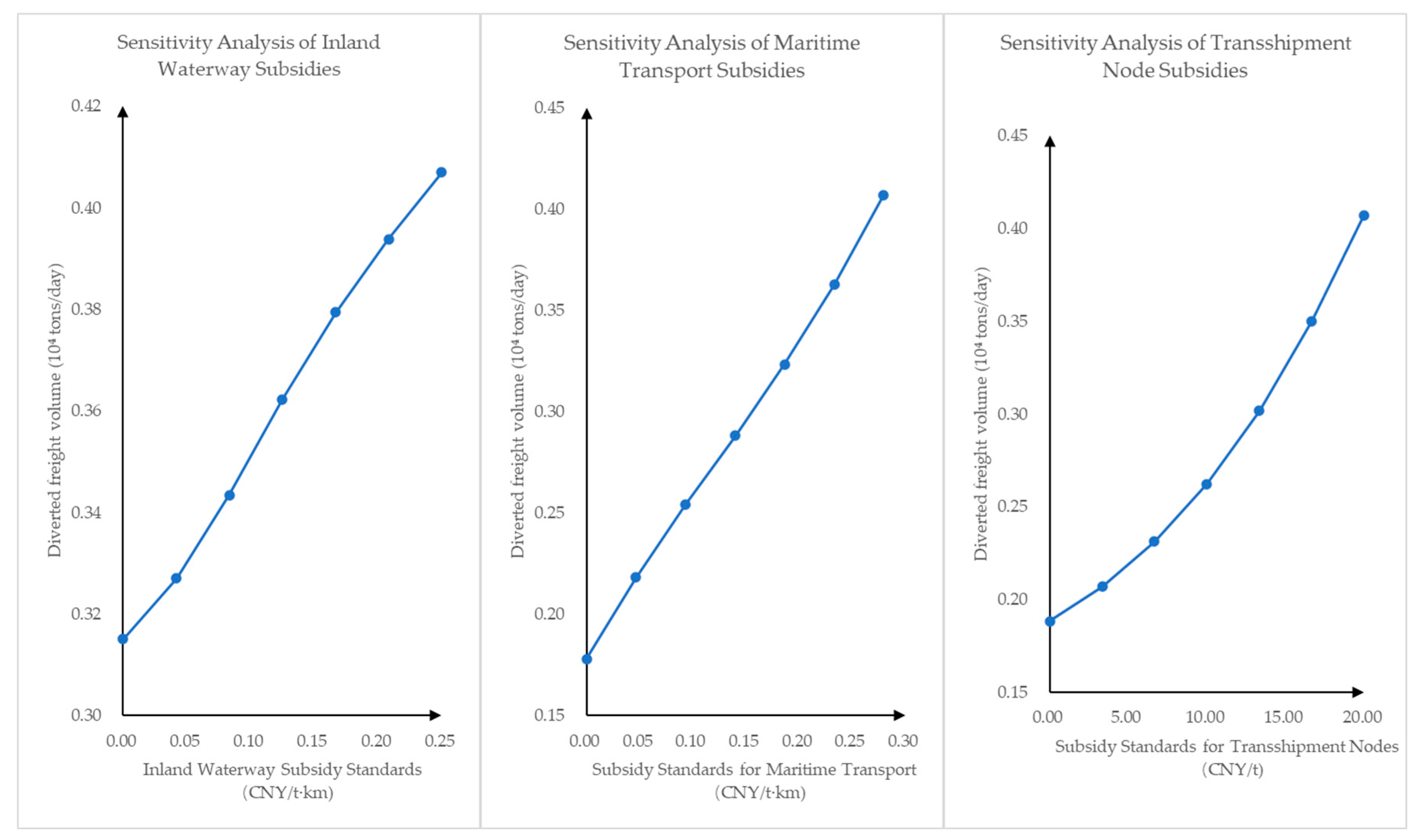
To reveal the influence mechanism of carbon subsidy policies on freight diversion, a sensitivity analysis was conducted on the inland waterway subsidy rate, maritime subsidy rate, and transshipment node subsidy rate. The results are presented in Figure 4:

(1)

Inland waterway subsidy sensitivity analysis

When the inland waterway subsidy rate was increased from 0 to 0.25 CNY/t·km, the waterway diversion volume rose from 3151 tons/day to 4070 tons/day, with a cumulative increase of 919 tons/day. On average, each increment of 0.01 CNY/t·km yielded approximately 38 tons/day of additional diversion. The diversion curve exhibited a nearly linear trend without an obvious marginal decline, indicating that the potential of inland waterway transport has not yet been fully realized. It is advisable to raise the inland waterway subsidy to its upper limit, subject to budget availability.

(2)

Maritime subsidy sensitivity analysis

When the maritime subsidy rate was increased from 0 to 0.28 CNY/t·km, the diversion volume grew from 1781 tons/day to 4070 tons/day, with a cumulative increase of 2289 tons/day. On average, each increment of 0.01 CNY/t·km generated approximately 79 tons/day of additional diversion, representing the highest efficiency among the three subsidy types. Since maritime routes are free from lock constraints and incur relatively low time costs, the subsidy can rapidly attract freight sources by directly reducing shipping prices, and thus should be deployed as the highest-priority subsidy instrument in the short term.

(3)

Transshipment node subsidy sensitivity analysis

When the transshipment subsidy rate was increased from 0 to 20 CNY/t, the diversion volume rose from 1883 tons/day to 4070 tons/day, with a cumulative increase of 2187 tons/day. The growth pattern exhibited distinct phases: the efficiency was moderate when the subsidy was below 10 CNY/t, whereas the diversion efficiency doubled once the subsidy exceeded 10 CNY/t. This indicates a policy threshold of 10 CNY/t for the transshipment subsidy. Below this threshold, the efficiency of fiscal expenditure is relatively low; it is therefore recommended that the initial transshipment subsidy rate should not be set lower than 10 CNY/ton.

6. Conclusions

Taking the road–waterway bimodal network in the Hangzhou Bay port area of Cixi as the research object, this study addresses the problems of an excessively high roadway transport share and insufficient momentum for waterway modal shift, and constructs a bi-level programming model for freight flow diversion on road–waterway bimodal networks considering carbon emissions. The main conclusions are as follows:

(1) The roadway–waterway bimodal network in the Ciyu region exhibits a structural contradiction characterized by overburdened roadways and underutilized waterways: roadway transport accounts for 94% of the regional freight volume, with the traffic load on critical segments reaching 0.78–0.79, while the waterway share remains extremely low. The impedance model developed in this study integrates the BPR function, the M/M/1 lock queuing model, and the M/M/c port handling queuing model into a unified framework, achieving an effective coupling between micro-level congestion effects and macro-level flow assignment.

(2) A bi-level programming model is constructed that combines the government’s differentiated subsidy decision-making with shippers’ flow assignment behavior, with the dual objectives of minimizing carbon emissions and subsidy expenditure. A nested algorithm combining NSGA-II and the Method of Successive Averages (MSA) is designed to solve the model. NSGA-II outperforms both NSGA and NSGA-III in terms of convergence (IGD = 0.0041), diversity (HV = 0.887), and computational efficiency.

(3) Carbon subsidy policies can effectively guide freight diversion, but an efficiency boundary exists. Without subsidies, the waterway share is merely 1.74%; under the medium subsidy cap, it rises to 22.70%, with cumulative emission reductions of 33.27 tons/day; when the daily subsidy exceeds CNY 350,000, the marginal diversion efficiency approaches zero. The subsidy strategy exhibits a three-stage evolutionary pattern: “prioritizing maritime shipping → jointly emphasizing inland and maritime shipping → shifting toward infrastructure investment at saturation.” The sensitivities of the three subsidy types differ significantly: the maritime subsidy shows the highest efficiency (79 tons/day per 0.01 CNY), followed by the inland waterway subsidy (38 tons/day per 0.01 CNY), while the transshipment subsidy exhibits a policy threshold of 10 CNY/t.

This study provides a quantitative analytical tool for designing differentiated subsidy policies to promote the roadway-to-waterway modal shift under limited fiscal resources. Future research can further investigate dynamic subsidy mechanisms, multi-agent game behavior, and the coupled mechanism of carbon taxes and carbon subsidies.

References

- Sheffi, Y. Urban Transportation Networks: Equilibrium Analysis with Mathematical Programming Methods; Prentice-Hall: Hoboken, NJ, USA, 1985. [Google Scholar]
- Spiess, H. Conical volume-delay functions. Transp. Sci. 1990, 24, 153–158. [Google Scholar] [CrossRef]
- Akcelik, R. A new look at Davidson’s travel time function. Traffic Eng. Control 1978, 19, 459–463. [Google Scholar]
- Davidson, K.B. The theoretical basis of a flow-travel time relationship for use in transportation planning. Aust. Road Res. 1978, 8, 32–35. [Google Scholar]
- Neuhold, R.; Fellendorf, M. Volume delay functions based on stochastic capacity. Transp. Res. Rec. 2014, 2421, 93–102. [Google Scholar] [CrossRef]
- Zhao, F.; Fu, L.; Zhong, M.; Liu, S.; Wang, X.; Huang, J.; Ma, X. Development and validation of improved impedance functions for roadways with mixed traffic using taxi GPS trajectory data and simulation. J. Adv. Transp. 2020, 2020, 7523423. [Google Scholar] [CrossRef]
- Zhang, A.; Zhang, Y.; Liu, Y. Low-carbon cold-chain logistics path optimization problem considering the influence of roadway impedance. IEEE Access 2023, 11, 124055–124067. [Google Scholar] [CrossRef]
- Mo, L.; Zhong, M.; Ma, X.F.; Liu, S.B.; Li, Y.Q. Research on freight impedance and distribution model of inland waterway in the Yangtze River based on ship AIS and visa data. J. Transp. Inf. Saf. 2017, 35, 98–106. [Google Scholar]
- Zheng, S.; Zhu, S.; Li, Z. Managing ship lock congestion in an inland waterway: A bottleneck model with a service time window. Transp. Policy 2021, 112, 142–161. [Google Scholar] [CrossRef]
- McFadden, D. Conditional logit analysis of qualitative choice behavior. In Frontiers in Econometrics; Zarembka, P., Ed.; Academic Press: Cambridge, MA, USA, 1974; pp. 105–142. [Google Scholar]
- Ye, X.; Yang, C.; Wang, T.; Yan, X.; Li, S.; Chen, J. Research on parking app choice behavior based on MNL. Travel Behav. Soc. 2021, 25, 174–182. [Google Scholar] [CrossRef]
- Ye, X.; Sui, X.; Wang, T.; Yan, X.; Chen, J. Research on parking choice behavior of shared autonomous vehicle services by measuring users’ intention of usage. Transp. Res. Part F Psychol. Behav. 2022, 88, 81–98. [Google Scholar] [CrossRef]
- Duncan, L.C.; Watling, D.P.; Connors, R.D.; Rasmussen, T.K.; Nielsen, O.A. Path Size Logit route choice models: Issues with current models, a new internally consistent approach, and parameter estimation on a large-scale network with GPS data. Transp. Res. Part B 2020, 135, 1–40. [Google Scholar] [CrossRef]
- Sun, Y.; Li, X. Fuzzy programming approaches for modeling a customer-centred freight routing problem in the road-rail intermodal hub-and-spoke network with fuzzy soft time windows and multiple sources of time uncertainty. Mathematics 2019, 7, 739. [Google Scholar] [CrossRef]
- Zhu, S.; Cai, Y.; Wang, M.; Wang, H.; Meng, Q. How will China–Singapore International Land–Sea Trade Corridor affect route choice behaviour? A discrete choice model. Transp. Policy 2023, 144, 11–22. [Google Scholar] [CrossRef]
- Li, X.; Xie, C.; Bao, Z. A multimodal multicommodity network equilibrium model with service capacity and bottleneck congestion for China-Europe containerized freight flows. Transp. Res. Part E 2022, 164, 102786. [Google Scholar] [CrossRef]
- Ye, X.; Zhu, Y.; Wang, T.; Yan, X.; Chen, J.; Zheng, P. Exploring the Effects of Shared Autonomous Vehicles and the Feasibility of a Novel Parking Pricing Policy: An Agent-Based Simulation Approach. IEEE Trans. Intell. Transp. Syst. 2025, 27, 2190–2202. [Google Scholar] [CrossRef]
- Tajtehranifard, H.; Bhaskar, A.; Nassir, N.; Haque, M.; Chung, E. A path marginal cost approximation algorithm for system optimal quasi-dynamic traffic assignment. Transp. Res. Part C 2018, 88, 91–106. [Google Scholar] [CrossRef]
- Batista, S.F.A.; Leclercq, L.; Menéndez, M. Dynamic Traffic Assignment for regional networks with traffic-dependent trip lengths and regional paths. Transp. Res. Part C 2021, 127, 103076. [Google Scholar] [CrossRef]
- Chandra, S.; Christiansen, M.; Fagerholt, K. Analysing the modal shift from road-based to coastal shipping-based distribution—A case study of outbound automotive logistics in India. Marit. Policy Manag. 2020, 47, 273–286. [Google Scholar] [CrossRef]
- Yin, C.; Ke, Y.; Chen, J.; Liu, M. Interrelations between sea hub ports and inland hinterlands: Perspectives of multimodal freight transport organization and low carbon emissions. Ocean Coast. Manag. 2021, 214, 105919. [Google Scholar] [CrossRef]
- Rudi, A.; Fröhling, M.; Zimmer, K.; Schultmann, F. Freight transportation planning considering carbon emissions and in-transit holding costs: A capacitated multi-commodity network flow model. EURO J. Transp. Logist. 2016, 5, 123–160. [Google Scholar] [CrossRef]
- Kundu, T.; Sheu, J.B. Analyzing the effect of government subsidy on shippers’ mode switching behavior in the Belt and Road strategic context. Transp. Res. Part E 2019, 129, 175–202. [Google Scholar] [CrossRef]
- Lu, I.J.; Lin, S.J.; Lewis, C. Decomposition and decoupling effects of carbon dioxide emission from highway transportation in Taiwan, Germany, Japan and South Korea. Energy Policy 2007, 35, 3226–3235. [Google Scholar] [CrossRef]
- Dai, Y.; Zhang, Z.; Zhao, Q. The combination of mega intermodal freight trains (MIFTs) and Mega Intermodal Hub (MIH) for intermodal transport. In CICTP 2012: Multimodal Transportation Systems; American Society of Civil Engineers: Reston, VA, USA, 2012; pp. 2037–2048. [Google Scholar]
- Alkaabneh, F.; Diabat, A.; Elhedhli, S. A Lagrangian heuristic and GRASP for the hub-and-spoke network system with economies-of-scale and congestion. Transp. Res. Part C 2019, 102, 249–273. [Google Scholar] [CrossRef]
- Ye, X.; Wang, Y.; Yan, X.; Wang, T.; Chen, J. Optimization model of autonomous vehicle parking facilities, developed with the nondominated sorting genetic algorithm with an elite strategy 2 and by comparing different moving strategies. IEEE Intell. Transp. Syst. Mag. 2022, 14, 2–20. [Google Scholar] [CrossRef]