The Dynamics of Digital Transformation: Why Similar Efforts Diverge

Abstract

Firms that invest similar amounts in digital transformation often end up with very different results: some achieve steady improvement, some remain at a low level, and others experience repeated rises and declines in performance. This study explains why these differences occur by examining technological innovation intensity, absorptive capacity, and operational performance as a connected process over time. Using a nonlinear dynamic model, we show that increasing technological innovation intensity does not guarantee better operational performance. Instead, outcomes depend on whether innovation activities are converted into absorptive capacity. When experience from innovation projects is absorbed and retained, absorptive capacity increases, and operational performance improves and remains stable. When this process is weak, firms may continue increasing innovation intensity, but absorptive capacity does not accumulate, and operational performance remains at a low level. We also find that as technological innovation intensity increases, more innovation activities take place at the same time, which raises coordination pressure. When coordination and management do not improve accordingly, the positive effect of absorptive capacity on operational performance becomes weaker, and performance may begin to rise and fall instead of improving steadily. In addition, the results show that firms need to reach a certain level of absorptive capacity before sustained improvement in operational performance can occur. Below this level, increasing technological innovation intensity alone does not change outcomes. At higher levels of absorptive capacity, operational performance may not always stabilize, but may instead fluctuate over time. These findings show that differences in digital transformation outcomes are not determined by technological innovation intensity alone, but by the joint dynamics of resource reconfiguration, learning accumulation, and coordination complexity, which shape absorptive capacity and operational performance over time.

1. Introduction

Digital transformation has become a central concern for firms seeking to improve competitiveness, resilience, and long-term performance [1,2,3]. It is not simply a matter of introducing digital tools or information systems. More often, it changes how work is organized, how information moves across units, and how decisions are coordinated inside the firm [4,5]. Yet firms that undertake similar digital initiatives do not necessarily obtain similar results. Some achieve sustained improvement, while others remain at a low level or move through repeated rounds of adjustment without stable gains [1,3]. The issue, then, is not whether digital transformation matters, but why similar efforts lead to different long-run outcomes.

Prior research does not fully answer this question. Existing studies have shown that digital transformation can improve firm performance and that organizational capability matters in this process [3]. What is less clear is how these effects build over time. Technological innovation activities, absorptive capacity, and performance are often discussed in separate streams, which makes it easier to identify their individual importance than to explain how they work together. As a result, the literature says relatively little about why some firms convert continuing digital initiatives into stable improvement, while others do not.

This gap matters because digital transformation does not unfold like a single innovation project. In many studies of technological innovation, innovation effort, capability, and performance can be examined as a relatively direct sequence. Digital transformation usually proceeds under different conditions. Firms often launch several initiatives at once, and these initiatives affect multiple systems, functions, and organizational units at the same time. Their effects therefore do not remain confined to the focal project. Instead, they alter adjacent processes, reshape cross-unit dependence, and increase the need for coordination as transformation expands. Under these conditions, the effect of technological innovation intensity on operational performance depends not only on the level of effort, but also on whether firms can absorb experience from multiple ongoing initiatives and coordinate an expanding set of interdependent changes. This is what distinguishes digital transformation from more general studies of technological innovation, where innovation efforts are more often treated as relatively discrete and self-contained [6]. For this reason, the relationship among technological innovation intensity, absorptive capacity, and operational performance in digital transformation cannot be reduced to a straightforward innovation–capability–performance sequence.

The paper examines digital transformation from this perspective. It focuses on how technological innovation intensity, absorptive capacity, and operational performance change over time when firms face growing coordination constraints. More specifically, the paper asks why similar levels of digital transformation effort can produce low-level persistence in some firms, sustained improvement in others, and repeated fluctuation in still others. To study this process, the paper develops a nonlinear dynamic model and uses scenario-based numerical analysis to trace how different organizational conditions lead to different long-run outcomes. An embedded case study is then used to compare the implications of the model with observed implementation patterns.

The analysis produces four main findings. First, digital transformation does not move firms along a single path. Even under similar external conditions, firms may remain at a low level, move toward sustained improvement, or experience repeated fluctuation. Second, technological innovation intensity improves operational performance only when experience from innovation activities is absorbed and retained so that absorptive capacity can build over time. The connection between technological innovation intensity and operational performance is therefore conditional on capability accumulation rather than generated by innovation effort alone [7]. Third, as more initiatives proceed in parallel, coordination pressure increases; if governance and coordination do not adjust accordingly, performance gains weaken and instability becomes more likely. In this sense, the contribution of absorptive capacity to operational performance also depends on whether coordination can be maintained as transformation expands. Fourth, digital transformation involves threshold effects: below a certain level of capability accumulation, increasing innovation intensity does not produce sustained improvement. Taken together, these findings suggest that digital transformation is not a linear process in which greater innovation effort steadily leads to better performance, but depends on whether innovation can be accumulated into absorptive capacity and sustained under increasing coordination pressure.

What the paper adds to the literature can be stated directly. The central insight of the model is that digital transformation outcomes are shaped not by innovation effort alone, but by whether innovation can be converted into absorptive capacity and whether that process can be sustained as coordination demands increase. It shows that digital transformation should not be treated as a standard innovation–capability–performance story. The simultaneity of multiple initiatives, the interdependence across systems and organizational units, and the coordination burden that grows with expansion change how technological innovation intensity, absorptive capacity, and operational performance relate to one another. The paper also explains why firms that appear to be making similar digital efforts can still end up in very different places: some remain stuck at a low level, some improve steadily, and some fluctuate as they expand. Finally, it shows why these differences are difficult to capture with static or linear approaches. A nonlinear dynamic framework makes it possible to identify threshold effects, low-level persistence, and recurrent fluctuation that would otherwise remain hidden. The study is theoretically grounded in three complementary perspectives. From the dynamic capabilities perspective, technological innovation intensity reflects firms’ efforts to reconfigure technological and organizational resources during digital transformation. From the organizational learning perspective, absorptive capacity represents the process through which experience from digital initiatives is accumulated, retained, and embedded into routines. From the complexity perspective, increasing coordination demands explain why digital transformation may generate nonlinear outcomes such as thresholds, path dependence, and recurrent fluctuation [8]. This theoretical positioning clarifies that the model is not only a methodological tool, but also a formal representation of the mechanisms through which digital transformation efforts produce divergent long-run outcomes.

To make the analytical focus of the study more explicit, this paper addresses two related research questions. First, why do firms undertaking similar digital transformation efforts experience different long-run outcomes, such as low-level persistence, sustained improvement, or repeated fluctuation? Second, how do technological innovation intensity, absorptive capacity, and operational performance interact over time as coordination demands increase during digital transformation? These questions guide the construction of the nonlinear dynamic model developed in the following sections.

The remainder of the paper is organized as follows. Section 2 reviews the literature on digital transformation, technological innovation intensity, absorptive capacity, and operational performance. Section 3 develops the nonlinear dynamic model and introduces the main assumptions. Section 4 presents the research design and embedded case. Section 5 reports the numerical analysis and main results. Section 6 discusses the managerial implications, and Section 7 concludes.

2. Literature Review

2.1. Digital Transformation as Organizational Reconfiguration

Digital transformation can no longer be reduced to the adoption of new information systems [9]. Recent studies define it more broadly as a process that reshapes strategy [10], organizational structure [11], internal processes, and governance arrangements. What is transformed is not only the technical infrastructure of the firm, but also the organizational arrangements through which technology is deployed and used [12]. However, existing research has mainly focused on three issues: technological innovation intensity absorptive capacity and organizational capability [13,14] and performance consequences. Most studies are designed to assess whether digital initiatives improve performance, but are less effective in explaining how such effects are generated and sustained over time. This study treats digital transformation as an organizational process rather than a discrete technological event and examines it through the interaction among technological innovation intensity, absorptive capacity, and operational performance.

2.2. Technological Innovation Intensity and Digital Transformation

Research on digital transformation has consistently shown that digital adoption and IT expenditure are associated with improvements in operational performance. Using regression models, quasi-experimental designs, and instrumental-variable approaches [6], prior studies estimate average effects and document variation across industries and governance contexts. These studies indicate that technological innovation intensity is a central component of digital transformation. In particular, firms’ efforts in digital technologies, information systems, and process innovation often initiate and shape transformation [15,16].

At the same time, the reported effects are uneven. Similar levels of technological innovation intensity do not always produce similar returns, and performance gains are not necessarily sustained. Industry conditions and resource endowments explain part of this variation, but they do not fully account for why firms operating under comparable conditions can follow different trajectories. Part of the difficulty lies in how this relationship is specified in the existing literature. Prior research often treats digital transformation efforts as an initial driver and performance as an outcome [17]. This specification is useful for showing whether digital transformation matters, but less useful for explaining what happens after implementation begins. Firms often revise the pace and scope of digital initiatives in light of observed results: early gains may encourage expansion, disappointing outcomes may prompt retrenchment, and competitive pressure may induce renewed efforts. When the influence of performance on subsequent transformation efforts is not incorporated into the analysis, these adjustments remain observable but insufficiently explained.

Related studies have also examined how digital initiatives reshape operational routines. Case-based and simulation studies show that automation, improved information flows, and data-driven decision-making can alter production organization and cross-functional coordination [17]. However, technological innovation intensity and capability development are rarely treated as interdependent processes. Existing research therefore establishes the importance of digital transformation, but provides a limited explanation of how innovation intensity interacts with capability development and performance over time.

2.3. Absorptive Capacity and Capability Dynamics

Research on absorptive capacity emphasizes organizational learning, knowledge integration, and adaptation as conditions for converting digital initiatives into effective organizational change. Empirical studies report mediating and moderating effects between digital investment and performance [14,18], while longitudinal case studies show how training, process redesign, data governance, and coordination practices support implementation. The above study points out that technological investment alone does not amount to digital transformation. Firms must also develop the capacity to absorb new knowledge, reconfigure routines, and align organizational practices with digital initiatives. Absorptive capacity is therefore not peripheral to digital transformation; it is one of the mechanisms through which digital initiatives become embedded in organizational practice and translated into operational outcomes.

However, absorptive capacity is often treated in static terms. It is commonly modeled either as a stable organizational attribute or as a mediator within a linear causal sequence [19]. Both approaches rest on restrictive assumptions: either capability remains broadly constant during the period of observation, or capability accumulation proceeds without significant erosion as initiatives expand [20]. This weakens the explanatory force of the literature, especially when the issue is why some firms convert digital initiatives into sustained improvement whereas others do not.

A different treatment is needed if transformation is understood as a process rather than an event. Capability accumulation is gradual, but it is not indefinitely self-reinforcing. As initiatives expand and interdependencies deepen, coordination demands increase, governance burdens intensify, and earlier learning gains may be offset. Unless absorptive capacity is specified as a state variable subject both to accumulation and to constraint, it is difficult to explain why some firms move beyond pilot implementation while others remain trapped in repeated but limited transformation efforts. Existing research therefore does not adequately capture the changing role of absorptive capacity in digital transformation over time.

2.4. Operational Performance and Feedback Dynamics

The performance consequences of digital transformation have also been extensively examined. Prior studies consistently associate digital capability with productivity, delivery speed, defect reduction, profitability, and resilience [21,22]. They further show that these effects vary with competitive intensity, market volatility, and supply-chain structure [23]. Other work considers competitive positioning and diffusion effects [24,25]. This literature leaves little doubt that operational performance is a central basis for assessing digital transformation. Operational outcomes indicate whether digital initiatives have been converted into organizational value. At the same time, such outcomes are not stable across all stages of implementation. Performance improvements are often strongest in earlier phases of digital expansion and may become less stable as implementation broadens and diffusion proceeds.

What receives less attention is the possibility that performance also shapes subsequent organizational choices [26]. In most studies, performance appears at the end of the causal chain [27]. Much less attention is given to how observed outcomes influence later investment decisions, implementation priorities, and organizational adjustment. That omission narrows the explanatory scope of the literature, since firms do not simply record outcomes; they revise their actions in response to them.

Without incorporating such feedback, prior research cannot explain when improvement becomes self-reinforcing, when it stalls, or when cyclical adjustment emerges. Similar investment trajectories may produce sustained gains in some firms and unstable outcomes in others, yet the mechanisms underlying these differences remain insufficiently specified. Operational performance has therefore been studied extensively as an outcome of digital transformation, but far less as a feedback mechanism within the transformation process itself.

2.5. The Modeling Gap

Existing research on digital transformation has mainly examined three issues: the intensity of firms’ digital innovation efforts, the role of absorptive capacity in implementing new technologies, and the effects of digital transformation on operational performance (

Table 1. Comparison between prior digital transformation research and this study.

Comparison Focus	Prior Digital Transformation Research	This Study
Research question	Prior studies mainly examine whether digital transformation improves firm performance or identify the conditions associated with successful transformation [7,21,28].	This study examines why firms undertaking similar digital transformation efforts may arrive at different outcomes.
Analytical perspective	Prior research often addresses technological innovation intensity, absorptive capacity, and operational performance separately, with limited attention to how they interact during the transformation process [6,22,29].	This study treats digital transformation as an organizational process shaped by the interaction among technological innovation intensity, absorptive capacity, and operational performance.
Methodological approach	Prior studies mainly rely on regression analysis, structural equation modeling, quasi-experimental designs, or mediation and moderation models to identify static or linear relationships [14,18,30].	This study adopts a nonlinear dynamic/system dynamics approach to examine feedback, stage-wise instability, and long-term change.
Treatment of key relationships	Prior research usually examines the effect of digital efforts on performance, the role of absorptive capacity in technology implementation, or the performance consequences of transformation, but rarely analyzes how these factors influence one another over time [8,31,32].	This study analyzes technological innovation intensity, absorptive capacity, and operational performance as interrelated components of the same transformation process.
Role of operational performance	Operational performance is mainly used to assess the outcome of digital transformation [21,22,23].	Operational performance is treated not only as an outcome, but also as a factor that shapes subsequent transformation efforts.
Overall contribution	Existing studies provide important evidence on digital transformation, organizational capability, and performance outcomes, but these lines of research remain loosely connected [6,25,33].	This study brings these strands together in a unified dynamic framework and explains how digital transformation develops over time and why similar efforts may produce different outcomes.

). However, these issues are usually addressed in separate strands of research or treated as part of a relatively direct causal sequence. Studies on technological innovation intensity tend to ask whether stronger digital efforts improve performance; studies on absorptive capacity mainly examine whether firms can absorb and apply new knowledge; and studies on operational performance typically assess whether digital transformation generates efficiency or competitive gains. Such work has established the importance of each factor, but it has not fully explained how these factors interact over time during digital transformation.

This limitation is theoretically important for two reasons. First, existing research on innovation and digital transformation has not sufficiently explained how technological innovation intensity, absorptive capacity, and operational performance shape one another across repeated rounds of implementation. In particular, prior studies rarely examine whether early performance outcomes affect later digital efforts, whether absorptive capacity changes as implementation expands, or how increasing coordination demands alter the relationship between transformation efforts and performance. Second, much of the literature still treats these relationships in relatively static or linear terms. As a result, prior research offers limited explanation of why firms with similar initial conditions and similar digital transformation efforts may arrive at different long-run outcomes, or why performance improvements observed in one stage may not be sustained in later stages.

This study addresses this limitation by analyzing technological innovation intensity, absorptive capacity, operational performance, and coordination complexity within a unified nonlinear dynamic framework. Conceptually, the framework connects three mechanisms that are central to digital transformation: resource reconfiguration, learning accumulation, and coordination complexity. From the perspective of dynamic capabilities, technological innovation intensity reflects firms’ efforts to reconfigure technological and organizational resources. From the perspective of organizational learning, absorptive capacity represents the accumulation and retention of implementation experience. From the perspective of complexity theory, simultaneous digital initiatives and cross-unit interdependence generate coordination pressure, threshold effects, and potential performance instability. By integrating these mechanisms, the study extends innovation research by showing that the relationship among innovation intensity, capability, and performance is conditional rather than fixed. It also contributes to digital transformation research by explaining why similar transformation efforts may lead to low-level persistence, sustained improvement, or recurrent fluctuation over time. Thus, the contribution of the model lies not simply in combining several variables, but in formalizing how capability reconfiguration, learning accumulation, and coordination complexity jointly shape divergent digital transformation trajectories.

2.6. Research Questions and Modeling Assumptions

Building on the above literature review and theoretical positioning, this study addresses two related research questions. First, why do firms undertaking similar digital transformation efforts experience different long-run outcomes, including low-level persistence, sustained improvement, and repeated fluctuation? Second, how do technological innovation intensity, absorptive capacity, and operational performance interact over time under increasing coordination pressure during digital transformation?

To address these questions, the model is developed on the basis of four modeling assumptions. First, technological innovation intensity does not influence operational performance in a purely direct and stable way; its effect depends on whether innovation efforts can be translated into absorptive capacity. Second, absorptive capacity is not treated as a fixed organizational attribute, but as a dynamic state variable that changes over time through both accumulation and constraint. Third, operational performance is not only an outcome of digital transformation, but also a feedback mechanism that influences subsequent innovation effort through organizational decision-making and resource allocation. Fourth, as multiple digital initiatives unfold in parallel, coordination complexity increases and weakens the stability of the relationship among innovation intensity, absorptive capacity, and operational performance.

These assumptions are not empirical hypotheses to be tested in a conventional statistical sense. It is also important to clarify the causal status of the model. The directional links specified in the system represent theoretically grounded mechanisms rather than empirically identified causal effects. The model assumes that technological innovation intensity, absorptive capacity, and operational performance influence one another through feedback relationships, but it does not estimate treatment effects or claim causal identification in the sense of experimental, quasi-experimental, or econometric causal inference designs. Instead, the purpose is to examine how the assumed mechanisms, once specified, generate different dynamic trajectories over time. Therefore, causal language in this study should be understood as model-implied and mechanism-based rather than as evidence of externally identified causal effects. Rather, they specify the structural conditions under which digital transformation is represented in this study as a nonlinear dynamic process. In this way, the model is designed to explain how interaction, feedback, and coordination pressure jointly produce divergent transformation trajectories over time.

3. Model Development

Digital transformation driven by technological innovation is a dynamic, process-based phenomenon rather than a one-shot mapping from investment to outcome. Firms often experience phases in which innovation effort expands, organizational pressure rises, performance fluctuates, and subsequent decisions are revised. In line with the research questions and modeling assumptions stated above, this study represents digital transformation as a nonlinear dynamic system with three time-varying state variables. Technological innovation intensity reflects resource reconfiguration from the dynamic capabilities perspective; absorptive capacity captures learning accumulation and knowledge retention from the organizational learning perspective; and operational performance represents the realized outcome of capability deployment. The nonlinear feedback and interaction terms capture coordination complexity, threshold effects, and potential instability. The model therefore formalizes how resource reconfiguration, learning accumulation, and coordination complexity jointly shape digital transformation over time.

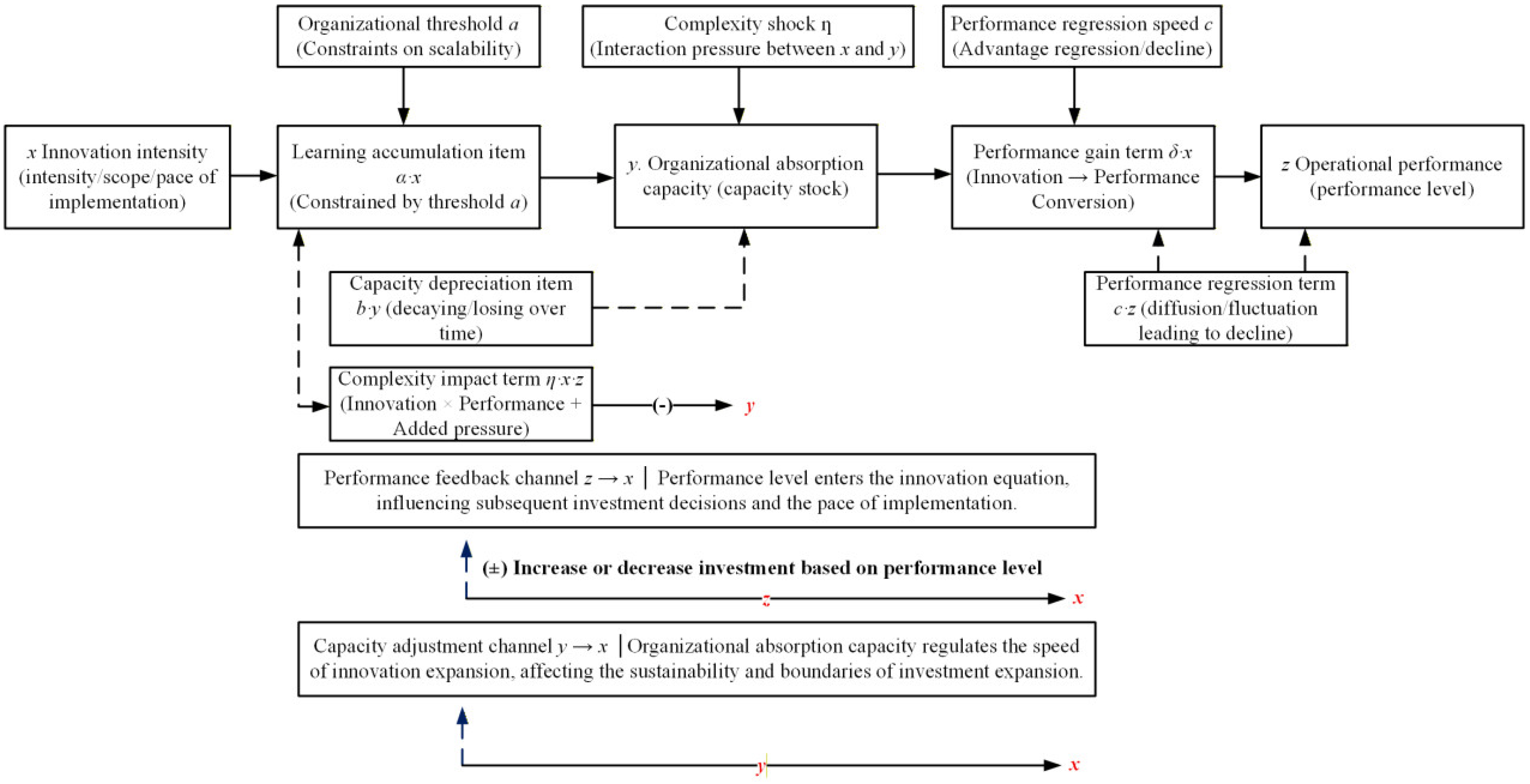
As shown in Figure 1, let $x\left(t\right)$ denote technological innovation intensity. It captures the scale and pace of innovation activities at time $t$. It covers the introduction of digital technologies, the deployment of information systems, and the execution of related projects. Let $y\left(t\right)$ denote organizational absorptive capacity. It reflects the firm’s ability to embed innovation into business processes, managerial routines, and coordination mechanisms. Let $z\left(t\right)$ denote operational performance. It summarizes performance in cost control, operating efficiency, delivery capability, and financial outcomes. These three states correspond to innovation action $x(t)$, organizational embedding capacity $y(t)$, and realized outcomes $z(t)$.

3.1. Innovation Intensity Dynamics

The evolution of innovation intensity reflects two forces. Consistent with the modeling assumptions above, innovation intensity is treated here as an adaptive variable rather than a fixed input, because firms revise transformation effort in response to observed outcomes. The first force is therefore performance feedback. When performance improves, resource and risk constraints typically ease. Managers become more willing to expand innovation efforts. When performance deteriorates, innovation projects are more likely to be postponed or scaled down. We therefore assume a positive association between the growth rate of innovation intensity and the current performance level $z(t)$.

The second force is the absorptive-capacity constraint. Scaling innovation requires organizational capacity. If capacity is weak, increasing project scale does not guarantee effective implementation. It may even reduce execution quality. To capture this constraint, we introduce a capability threshold $a$. It represents the minimum absorptive capacity required to support expansion. We use the term $\left(y(t)-a\right)x(t)$ to represent how absorptive capacity affects the expansion speed of innovation intensity. When $y(t)>a$, the term is positive and supports expansion. When $y(t)<a$, the term is negative and suppresses expansion. Accordingly, the dynamic equation for innovation intensity is specified as ${\displaystyle \frac{dx(t)}{dt}}=z(t)+(y(t)-a)x(t)$. This specification implies that the expansion of technological innovation intensity is jointly shaped by current performance and organizational carrying capacity. Stronger performance relaxes resource and risk constraints and thus supports further innovation effort. At the same time, expansion depends on whether absorptive capacity has reached the threshold required to sustain a larger implementation scale. When absorptive capacity remains below that threshold, continued expansion becomes difficult and may even be reversed. The equation therefore reflects a recurrent feature of digital transformation: firms may be willing to intensify innovation when current results are favorable, but the pace of expansion ultimately depends on whether the organization is capable of supporting and absorbing that increase. The equation therefore links innovation expansion to both performance feedback and absorptive-capacity conditions. Performance raises (or relaxes) the willingness and ability to invest. Absorptive capacity determines whether expansion is feasible and whether it accelerates or stalls.

3.2. Dynamics of Organizational Absorptive Capacity

Absorptive capacity is modeled here as a dynamic state variable rather than a fixed organizational characteristic, because digital transformation requires cumulative learning and organizational embedding, while the effect of such learning may weaken as coordination demands intensify. Organizational absorptive capacity is treated as a stock that evolves with implementation practice. It increases when firms repeatedly translate innovation activities into process adjustments, skill upgrading, and data-governance improvements. We model this accumulation as proportional to innovation intensity. The term $\alpha x(t)$ captures the contribution of innovation activity to capability formation. Absorptive capacity also depreciates. Interruptions in practice, turnover of key personnel, and loss of experiential knowledge reduce the usable stock of capability. We represent this effect with a proportional decay term, $-by\left(t\right)$. Beyond accumulation and depreciation, absorptive capacity may be weakened when innovation scale and performance pressure rise simultaneously. High innovation intensity often entails greater project parallelism, tighter evaluation cycles, and heavier coordination demands. As interdependencies increase, coordination costs rise and the organization’s ability to embed innovation into routines can be impaired. To capture this joint strain, we introduce an interaction term, $-\eta x(t)z(t)$. It represents the additional loss in absorptive capacity associated with the combined effect of innovation expansion and performance pressure. Accordingly, the evolution of absorptive capacity is specified as ${\displaystyle \frac{dy(t)}{dt}}=\alpha x(t)-by(t)-\eta x(t)z(t)$. This equation treats absorptive capacity as an evolving organizational stock rather than a fixed attribute. It increases when innovation activities generate experience that can be retained and embedded into routines, skills, and governance arrangements. It also depreciates when earlier learning is not sustained in practice. In addition, capability formation may be weakened when innovation expansion coincides with rising performance pressure, since the organization must then absorb new experience under more demanding coordination conditions. The equation thus formalizes a central point of the paper: absorptive capacity develops through repeated learning, but its accumulation can be interrupted or offset when the pace of transformation exceeds the organization’s ability to embed and coordinate change.

3.3. Dynamics of Operational Performance

Operational performance is specified not only as an outcome of transformation activities, but also as part of the dynamic process, because observed performance influences later organizational decisions and the continuation of innovation effort. Operational performance improves through innovation-driven changes in production and coordination. Digital technologies support automation, reduce information frictions, and enable process optimization and data-informed decision-making. We therefore specify a positive contribution from innovation intensity to performance growth. The term $\delta x(t)$ captures this effect. Performance gains are not fully persistent. Competitive imitation, diffusion of similar practices, and changing environmental conditions erode initial advantages and create a tendency for performance to revert. We represent this tendency with a linear reversion term, $-cz\left(t\right)$. The resulting performance dynamics are ${\displaystyle \frac{dz(t)}{dt}}=\delta x(t)-cz(t)$. This specification assumes that technological innovation intensity contributes positively to operational performance by improving process efficiency, coordination, and execution quality. However, such gains are not fully self-sustaining. Competitive imitation, diffusion of similar practices, and the erosion of early advantages create pressure for performance to revert. Operational improvement should therefore be understood as contingent rather than permanent. The equation captures this point by allowing innovation to raise performance while also recognizing that those gains may weaken over time if they are not continually reinforced through subsequent transformation efforts.

Together with the innovation-intensity equation in Section 3.1, these specifications yield a closed dynamic system for $\left\{x\left(t\right),y\left(t\right),z\left(t\right)\right\}$, which is used in subsequent analysis to characterize long-run states, threshold effects, and the conditions under which trajectories diverge or become oscillatory.

Accordingly, the innovation-driven digital transformation dynamics can be written as the following nonlinear system:

$$\left\{\begin{array}{c}{\displaystyle \frac{dx(t)}{dt}}=z+(y-a)x\\ {\displaystyle \frac{dy(t)}{dt}}=\alpha x-by-\eta xz\\ {\displaystyle \frac{dz(t)}{dt}}=\delta x-cz\end{array}\right.$$

All parameters as shown in

Table 2. Parameter.

Type	Symbol	Definition	Indicator Sources
State variable	$x(t)$	Innovation intensity	PMO/project registry: number of concurrent projects, go-live counts, iteration frequency, milestone completion. Finance/budget: digital/IT spending intensity (share or growth rate).
	$y(t)$	Absorptive capacity	HR/L&D: training coverage, role certification rate. BPM/process office: process standardisation progress, SOP update records. Data governance: data quality score, master-data consistency, governance compliance rate.
	$z(t)$	Operating performance	ERP/BI dashboards: unit cost, productivity measures. Supply chain/delivery: lead time, on-time delivery. MES/quality: defect rate, rework rate. Finance: margin or operating profit contribution (optional).
Parameter	$a$	Organisational threshold for scaling innovation	Calibrated from Firm A. Anchored to periods where scaling stalled despite project effort. Linked to low process/data readiness.
	$b$	Depreciation rate of absorptive capacity	HR: turnover in key roles, replacement cycle time. L&D: re-training frequency. Estimated from declines in $y(t)$ during low-activity periods.
	$c$	Reversion speed of performance	Operations/finance dashboards: speed of performance decay when innovation effort weakens. Estimated from reversion segments of $z(t)$.
	$\alpha$	Learning efficiency from innovation to capacity	Estimated from co-movement between project activity $x(t)$ and capacity gains $y(t)$. Supported by training and process-change records.
	$\eta$	Complexity shock on capacity (interaction effect)	PMO/collaboration tools: parallel project load, change requests, ticket backlog. Performance management: target pressure proxies. Calibrated from capacity drops when $x(t)$ and $z(t)$ are both high.
	$\delta$	Conversion efficiency from innovation to performance	Estimated from the performance equation linking changes in $z(t)$ to $x(t)$ and the reversion term. Grounded in KPI improvements tied to deployments.

, and are assumed to be positive: $a>0,\alpha >0,b>0,\eta >0,\delta >0,c>0$. In this system, innovation intensity $x(t)$ increases absorptive capacity through $\alpha x(t)$ and improves operational performance through $\delta x(t)$. Performance $z(t)$ enters the innovation equation and thus affects subsequent innovation expansion. Absorptive capacity $y(t)$ regulates the growth of innovation via $\left(y(t)-a\right)x(t)$, capturing a threshold effect around $a$. The interaction term $-\eta x(t)z(t)$ represents the additional strain on capability formation when innovation scale and performance pressure rise jointly. Each component corresponds to a mechanism observed in firms’ digital transformation practice, providing a parsimonious yet interpretable basis for the subsequent analysis of equilibria and stability. The three equations describe digital transformation as a mutually connected process rather than a one-directional sequence. Technological innovation intensity affects both absorptive capacity and operational performance; operational performance feeds back into subsequent innovation expansion; and absorptive capacity both supports and constrains the continuation of innovation effort. At the same time, coordination pressure enters the process by weakening capability formation when innovation expansion and performance pressure rise jointly. This structure makes it possible to examine why firms with comparable initial conditions may nevertheless move toward different long-run outcomes, including low-level persistence, sustained improvement, or repeated fluctuation.

4. Equilibrium Analysis

Theorem 1. 

Consider the technological innovation system  $\left\{\begin{array}{c}\stackrel{•}{x}=z+(y-a)x\\ \stackrel{•}{y}=\alpha x-by-\eta xz\\ \stackrel{•}{z}=\delta x-cz\end{array}\right.$, if $\Delta ={\alpha }^2-{\displaystyle \frac{4\eta \delta b(ac-\delta )}{c^2}}\ge 0$, then the system admits exactly three equilibrium points, $E_1=(0,0,0)$, $E_2=\left({\displaystyle \frac{\alpha c+\sqrt{{\alpha }^2{c}^2-4\eta \delta bac+4\eta {\delta }^{2}b}}{2\eta \delta }},a-{\displaystyle \frac{\delta }{c}},{\displaystyle \frac{\alpha c\delta +\delta \sqrt{{\alpha }^2{c}^2-4\eta \delta bac+4\eta {\delta }^{2}b}}{2\eta \delta c}}\right)$, $E_3=\left({\displaystyle \frac{\alpha c-\sqrt{{\alpha }^2{c}^2-4\eta \delta bac+4\eta {\delta }^{2}b}}{2\eta \delta }},a-{\displaystyle \frac{\delta }{c}},{\displaystyle \frac{\alpha c\delta -\delta \sqrt{{\alpha }^2{c}^2-4\eta \delta bac+4\eta {\delta }^{2}b}}{2\eta \delta c}}\right)$. Otherwise, then the system has a unique equilibrium point, namely the origin $E_1=(0,0,0)$.

E1 represents a state of innovation stagnation in which digitalization is effectively inactive: $x=0$ indicates that the firm has largely ceased proactive technological innovation and digital project execution; $y=0$ implies that absorptive capacity is no longer reinforced through practice and gradually decays to a very low level; and $z=0$ denotes a return to a baseline performance level (normalized to zero in the model), so innovation neither raises performance nor materially worsens it. Organizationally, this corresponds to a cautious or conservative stance toward digitalization—often after earlier attempts yielded limited learning gains under high coordination complexity and weak internal alignment, prompting the firm to scale back and revert to established routines. By contrast, E2 captures a high-innovation–high-performance steady state: the firm sustains relatively high innovation investment and project execution, organizational capacity stabilizes at a level sufficient to support this pace through accumulated learning, and innovation outcomes translate into performance in a relatively consistent manner; empirically, such firms tend to develop a more mature digital operating system, with continuous upgrading, standardized processes and data governance, and a close fit between innovation rhythm and organizational carrying capacity. E3, finally, corresponds to a low-innovation–moderate-performance long-run state: the firm does not abandon digitalization but maintains limited, conservative innovation activity, absorptive capacity remains around the threshold yet does not support expansion, and performance improves only modestly relative to a traditional mode without producing a pronounced advantage; many firms can remain in this regime for extended periods, with some systems and localized gains but no step change in overall performance, which in turn sustains managerial caution toward further increases in innovation investment.

Theorem 2. 

Consider the technological innovation system, (i) If  $ac>\delta$, the equilibrium E1 is locally asymptotically stable. (ii) If  $ac<\delta$, the equilibrium E1 is unstable.

When $ac>\delta$, the system exhibits a conservative stability configuration. A high organizational threshold $a$, a fast reversion rate $c$, and limited innovation-to-performance conversion $\delta$ make it easy for the firm to remain near a low-innovation equilibrium. Small-scale pilots are then unlikely to initiate a substantive transformation trajectory. By contrast, when $ac<\delta$, the system takes on an innovation-amplifying structure. In this case, the “no-innovation” state is not robust: once innovation activity is initiated, the dynamics are more likely to move toward a sustained transformation path. From a managerial perspective, escaping a prolonged regime of sporadic innovation and overall stagnation therefore requires interventions on two margins. One is to reduce the organizational threshold $a$ and the speed of performance reversion $c$, for example by standardizing processes and reducing short-term performance pressure in evaluation systems. The other is to increase the conversion efficiency $\delta$, for example by concentrating innovation on high-value use cases and strengthening implementation quality. These adjustments shift the system from a region in which the origin is locally stable to one in which the origin becomes unstable, thereby creating conditions for sustained innovation and transformation.

Theorem 3.

The equilibrium point E2 is locally asymptotically stable if the following three inequalities hold simultaneously:

(i) 

$c-a+{\displaystyle \frac{2\delta }{c}}>0$;

(ii) 

$b(\delta -ac)+\delta \eta {\left({\displaystyle \frac{\alpha c+\sqrt{{\alpha }^2{c}^2-4\eta \delta bac+4\eta {\delta }^{2}b}}{2\eta \delta }}\right)}^2>0$;

(iii) 

$b\left(b+c+{\displaystyle \frac{\delta }{c}}\right)\left(c-a+{\displaystyle \frac{2\delta }{c}}\right)>b(\delta -ac)+\delta \eta {\left({\displaystyle \frac{\alpha c+\sqrt{{\alpha }^2{c}^2-4\eta \delta bac+4\eta {\delta }^{2}b}}{2\eta \delta }}\right)}^2$.

A high-innovation equilibrium is not inherently stable. Even when a firm has the prerequisites for a “high innovation–high performance” regime, the equilibrium may remain unstable if performance adjustment is sluggish, the organizational threshold is high, or the complexity shock is strong. Under such conditions, an initial surge in innovation can be followed by forced retrenchment, and the firm may drift back toward a low-innovation level. Stability of the high-innovation regime requires three conditions to hold jointly. First, the organizational threshold must be commensurate with the speed of performance adjustment (Condition (i)), avoiding the combination of a high threshold and slow adjustment. Second, capability depreciation and complexity shocks must not dominate the positive accumulation generated by innovation (Condition (ii)). Third, the system must possess sufficient “damping capacity”—in the form of process standardization, governance capability, and effective coordination mechanisms—to attenuate fluctuations under high innovation (Condition (iii)). Accordingly, firms seeking to sustain a high level of innovation and digitalization over the long run must do more than improve the quality and returns of innovation itself (as captured by $\delta$ and $\alpha$). They also need to lower the organizational threshold $a$ (e.g., by preparing processes and talent in advance), contain complexity and project parallelism (thereby reducing the effective impact of $\eta$ and the intensity of expansion), and strengthen damping through institutional and governance arrangements (affecting $b$, $c$, and the implied adjustment strength represented by $b+c+\delta /c$). Only when these dimensions improve in concert can the high-innovation equilibrium E2 become a durable long-run destination of digital transformation rather than a transient peak.

Theorem 4. 

The equilibrium point E3 is locally asymptotically stable if the following inequalities are satisfied: (i)  $b(ac-\delta )-\delta \eta {\left({\displaystyle \frac{\alpha c-\sqrt{{\alpha }^2{c}^2-4\eta \delta bac+4\eta {\delta }^{2}b}}{2\eta \delta }}\right)}^2>0$; (ii) $b\left(b+c+{\displaystyle \frac{\delta }{c}}\right)\left(c+a\right)>b(ac-\delta )-\delta \eta {\left({\displaystyle \frac{\alpha c-\sqrt{{\alpha }^2{c}^2-4\eta \delta bac+4\eta {\delta }^{2}b}}{2\eta \delta }}\right)}^2$.

A “limited-innovation, limited-return” trajectory can be dynamically robust. Once Conditions (i)–(ii) hold, a firm may temporarily intensify innovation efforts or realize a modest performance uptick, yet it can still be pulled back quickly to the original low-innovation regime under the joint effects of a high organizational threshold, capability depreciation, and performance pressure. This robustness reflects, first, strong organizational and performance constraints (i.e., relatively large $a$, $b$, and $c$); and second, a complexity shock that remains too weak to disrupt the incumbent structure, which is captured by a relatively small value of $\eta {\displaystyle \frac{\alpha c-\sqrt{{\alpha }^2{c}^2-4\eta \delta bac+4\eta {\delta }^{2}b}}{2\eta \delta }}$.

In practical terms, firms in this regime often “do not perform poorly, yet struggle to move beyond incremental progress,” and may therefore remain around this level for a prolonged period. To escape such a stable low-level regime, the structure implied by the analytical conditions points to two complementary levers. The first is to attenuate the forces that stabilize the low-innovation equilibrium—for example, lowering an excessively high organizational threshold $a$, easing avoidable short-term performance pressure (thereby reducing $c$), and mitigating capability depreciation through capability management (reducing $b$). The second is to increase the substantive change effect of innovation activity and the effective impact of the complexity-related mechanism—by appropriately raising $\delta$ and $\eta$, or by improving the quality (rather than merely the scale) of transformation so as to increase ${\displaystyle \frac{\alpha c-\sqrt{{\alpha }^2{c}^2-4\eta \delta bac+4\eta {\delta }^{2}b}}{2\eta \delta }}$. These adjustments can render the original low-innovation equilibrium unable to satisfy Conditions (i)–(ii), thereby opening a pathway toward the high-innovation equilibrium E2 or, potentially, toward more complex dynamic regimes.

Assume $ac>\delta$, define ${\alpha }_{SN}={\displaystyle \frac{2}{c}}\sqrt{\eta \delta b(ac-\delta )}$, and, for $\alpha >{\alpha }_{SN}$, ${\Phi }_2(\alpha )=b(ac-\delta )-\delta \eta {\left({\displaystyle \frac{\alpha c+\sqrt{{\alpha }^2{c}^2-4\eta \delta bac+4\eta {\delta }^{2}b}}{2\eta \delta }}\right)}^2-(b+c+{\displaystyle \frac{\delta }{c}})b(a+c)$, ${\Phi }_3(\alpha )=b(ac-\delta )-\delta \eta {\left({\displaystyle \frac{\alpha c-\sqrt{{\alpha }^2{c}^2-4\eta \delta bac+4\eta {\delta }^{2}b}}{2\eta \delta }}\right)}^2-(b+c+{\displaystyle \frac{\delta }{c}})b(a+c)$, suppose that ${\Phi }_2(\alpha )$ has a unique positive root on $\left({\alpha }_{SN},\infty \right)$, denoted ${\alpha }_{H_2}$; ${\Phi }_3(\alpha )$ has a unique positive root on $\left({\alpha }_{SN},\infty \right)$, denoted ${\alpha }_{H_3}$, and that the transversality conditions ${\displaystyle \frac{d}{d\alpha }}{\Phi }_2({\alpha }_{H_2})\ne 0$, ${\displaystyle \frac{d}{d\alpha }}{\Phi }_3({\alpha }_{H_3})\ne 0$ hold. Then the system exhibits the following qualitative dynamics as $\alpha$ varies:

Theorem 5. 

(Region I) If  $0<\alpha <{\alpha }_{\mathrm{SN}}$, the system admits a unique equilibrium, the origin E1. (Region II) At  $\alpha ={\alpha }_{\mathrm{SN}}$, the system undergoes a saddle–node bifurcation at the non-trivial equilibria, and a pair of equilibria E2 and E3 is created. (Region III) If  ${\alpha }_{\mathrm{SN}}<\alpha <{\alpha }_{H_2}$, the system has three equilibria E1, E2, E3; the origin E1 is unstable, while both non-trivial equilibria E2 and E3 are locally asymptotically stable. (Region IV) At  $\alpha ={\alpha }_{H_2}$, the equilibrium E2 loses stability via a Hopf bifurcation. (Region V) If  ${\alpha }_{H_2}<\alpha <{\alpha }_{H_3}$, the equilibrium E2 is unstable, whereas E3 remains locally asymptotically stable. (Region VI) At  $\alpha ={\alpha }_{H_3}$, the equilibrium E3 loses stability via a Hopf bifurcation. (Region VII) If  $\alpha >{\alpha }_{H_3}$, the origin E1 is unstable and both non-trivial equilibria E2 and E3 are unstable.

In the model, $\alpha$ measures the efficiency with which innovation practice is converted into organizational absorptive capacity. A larger $\alpha$ means that each unit of innovation activity yields more usable capability in routines, skills, and data governance. A smaller $\alpha$ means that projects are executed but little capability is retained. Theorem 5 partitions $\alpha$ into seven regimes. Each regime corresponds to a distinct long-run dynamic pattern. Together they describe typical digital-transformation trajectories under different levels of “learning efficiency.”

(1) Low-$\alpha$ regime with negligible transformation (Region I): When $0<\alpha <{\alpha }_{SN}$, the system admits only one equilibrium, E1 = (0, 0, 0). As shown in Theorem 2, under $ac>\delta$ this equilibrium can be locally stable. Firms may run scattered technical trials. Learning is too weak to accumulate capability. Innovation cannot be sustained. The system returns to a near–no-innovation state. Digitalization remains at the pilot level. (2) The threshold $\alpha ={\alpha }_{SN}$ and the emergence of transformation alternatives (Region II): At $\alpha ={\alpha }_{SN}$, a saddle-node bifurcation occurs. Two nonzero equilibria, E2 and E3, are created. Once learning efficiency reaches this threshold, two self-sustaining development modes become feasible. One is a relatively high-innovation path E2. The other is a relatively low-innovation path E3. The system moves from a single “non-transformation” attractor to a setting with multiple feasible paths. (3) Intermediate $\alpha$ with path dependence and bistability (Region III): When ${\alpha }_{SN}<\alpha <{\alpha }_{H_2}$, the system has three equilibria. Both nonzero equilibria E2 and E3 are locally asymptotically stable. This is a standard path-dependent configuration. Under the same industry and macro environment, some firms converge to the high-innovation–high-performance state E2. Others settle into the low-innovation state E3 with limited improvement. Which outcome prevails depends on early choices. Pilot design matters. Early results matter. Managerial tolerance for failure matters. This regime matches the empirical pattern in which firms face similar opportunities yet diverge markedly. (4) $\alpha ={\alpha }_{H_2}$ and the onset of oscillation around the high-innovation state (Region IV): At $\alpha ={\alpha }_{H_2}$, equilibrium E2 loses stability via a Hopf bifurcation. A periodic orbit emerges around it. Learning efficiency continues to rise. Governance, processes, and coordination do not keep pace. The high-innovation–high-performance mode becomes unstable. Innovation effort and performance begin to cycle. In practice, this resembles repeated “push hard, then pull back” episodes at relatively high innovation levels. The system no longer settles into a stable new steady state.

(5) ${\alpha }_{H_2}<\alpha <{\alpha }_{H_3}$ with an unstable high-innovation state and a stable conservative state (Region V): In this interval, E2 is unstable, while E3 remains stable. Higher learning efficiency does not guarantee a stable high-innovation regime. Sustained high innovation becomes hard to maintain. The conservative, low-innovation mode becomes the stable outcome. Empirically, some firms attempt an intensive transformation wave. Organizational load becomes excessive. Pace is too fast. Projects are cut back. The firm returns to a controllable but conservative level. That regime is “comfortable” organizationally and therefore persistent. (6) $\alpha ={\alpha }_{H_3}$ and oscillation around the conservative state (Region VI): At $\alpha ={\alpha }_{H_3}$, equilibrium E3 also loses stability through a Hopf bifurcation. The implication is stronger. Even the “limited innovation, limited return” mode cannot remain stable. Cycles can arise around either innovation level. This corresponds to a situation in which firms feel compelled to transform, yet no innovation level yields a stable operating point. Too little transformation invites external pressure. Too much creates internal instability. Strategic oscillation becomes difficult to avoid.

(7) $\alpha >{\alpha }_{H_3}$ and complex dynamics (Region VII). When $\alpha >{\alpha }_{H_3}$, all three equilibria are unstable: The system moves in periodic or more complex motions around their neighborhoods. Very high learning efficiency, without concurrent upgrading of governance and institutional arrangements, can produce persistent high-frequency adjustment. The organization may display strong innovative energy. It also faces higher managerial costs and uncertainty. The bifurcation analysis therefore implies that higher $\alpha$ is not unconditionally beneficial. If $\alpha$ is too low, no sustainable transformation path emerges. If $\alpha$ is moderate, high- and low-innovation regimes coexist and path dependence dominates. If $\alpha$ rises further, Hopf bifurcations can generate persistent oscillations. High- and then low-innovation equilibria lose stability. The system enters a complex regime characterized by frequent adjustment.

For brevity, detailed mathematical derivations and theorem proofs are provided in Appendix A.

5. Numerical Analysis and Empirical Validation

This section presents the numerical analysis and empirical calibration used to examine the model in a real organizational setting. Guided by the research questions stated above, the analysis focuses on whether similar levels of digital transformation effort can lead to different long-run outcomes, and how such divergence emerges through the interaction among technological innovation intensity, absorptive capacity, operational performance, and coordination complexity.

The numerical study is anchored in a manufacturing firm, referred to as Firm A, which is undergoing active digital transformation and maintains traceable internal records, including digital project logs, capability-building documents, and operational performance dashboards. Firm A is used as an empirical anchor rather than as a statistically representative sample. The calibration exercise is therefore not intended as a causal identification strategy. Its purpose is to construct plausible state variables and parameter values for the dynamic system, not to isolate exogenous variation or estimate causal treatment effects.

The analysis examines whether the proposed nonlinear dynamic structure can plausibly reproduce and interpret the transformation patterns observed within the firm. Accordingly, the findings should be understood as analytically generalizable at the level of underlying mechanisms, rather than as statistically generalizable results or directly transferable parameter estimates. In the following analysis, equilibrium states are interpreted as distinct organizational regimes, and bifurcation points are interpreted as thresholds at which the qualitative behavior of transformation changes.

We use three types of internal records. (i) Innovation and digital project records: project go-live dates and iteration pace, the number of projects running in parallel, and measures of digital investment intensity. (ii) Learning and absorptive-capacity records: training coverage, competence attainment in key roles, progress in process standardization and data governance, and the closure of cross-functional coordination loops. (iii) Operational performance records: cost efficiency, delivery performance, quality performance, and profitability.

Based on these observable indicators, we construct the three state variables $x\left(t\right)$, $y\left(t\right)$, and $z\left(t\right)$. They represent, respectively, innovation intensity, absorptive capacity, and operational performance at time $t$. Construction relies on logs and dashboards rather than subjective ratings. Although the construction of x, y, and z relies on traceable organizational records rather than subjective ratings, these variables should still be interpreted as proxies for broader theoretical constructs. Project counts, go-live records, and digital investment intensity capture important aspects of technological innovation intensity, but may not fully reflect the novelty, difficulty, or implementation quality of digital initiatives. Training coverage, certification rates, process standardization, and data-governance indicators approximate absorptive capacity, but they may overlook tacit knowledge, informal learning, cross-functional trust, and employees’ willingness to apply new knowledge. Operational performance indicators such as cost efficiency, delivery reliability, defect rates, and profitability may also be affected by demand conditions, input prices, supply-chain disruptions, or managerial interventions. Future research could use alternative or complementary proxies, including digital patents, system integration depth, digital process redesign, knowledge-sharing networks, collaboration records, internal knowledge-reuse rates, survey-based learning measures, customer satisfaction, service reliability, and resilience indicators. Combining archival records, surveys, and process-tracing data would help reduce measurement bias and strengthen construct validity.

The construction of these variables is intended to map observable operational records onto the conceptual state variables defined in the model, ensuring consistency between theoretical constructs and empirical representation.

The raw series are preprocessed to reduce measurement noise and make them comparable across units. We handle missing values, winsorize extreme observations, and apply smoothing and frequency alignment when needed. We then transform $x_{raw}(t)$, $y_{\mathrm{raw}}(t)$, and $z_{\mathrm{raw}}(t)$ into unit-free series $x\left(t\right)$, $y\left(t\right)$, and $z\left(t\right)$ using standard scaling (e.g., min–max normalization or indexing to a base period). After this step, each variable tracks relative changes over the sample period. The common scale improves comparability across variables and stabilizes numerical solution of the dynamic system.

Calibration uses Firm A’s discrete-time observations. Because the data are observed at discrete intervals, we approximate the time derivatives $\dot{x}(t_i)$, $\dot{y}(t_i)$, and $\dot{z}(t_i)$ with finite differences and estimate the model based on these constructed rates of change. We adopt a “single-equation first, joint calibration next” strategy. The third equation is linear in $(\delta ,c)$, so we estimate it first to strengthen identification. We then estimate the remaining parameters under positivity constraints $a,b,c,\eta ,\delta >0$ using constrained least squares or nonlinear least squares, and we check robustness using weighted specifications or robust standard errors. This procedure ties each parameter to observed movements in Firm A’s series rather than selecting values for analytical convenience.

Based on the calibration results and the scaled units, we use the following baseline parameter set for simulation: $a=1.0,b=1.0,c=1.0,\eta =0.2,\delta =0.5$. These values are representative of Firm A’s calibrated estimates after normalization. They summarize the relative strength of organizational thresholds, capability depreciation, performance reversion, complexity shocks, and innovation returns in the study period. The baseline also satisfies the structural conditions required in the theoretical analysis (e.g., $ac>\delta$). When selecting ranges for $\alpha$, we ensure that the discriminant satisfies $\Delta \ge 0$ so that nonzero equilibria exist, which allows the bifurcation and stability results to be evaluated in the empirical context of Firm A.

We solve the system using standard numerical integration for ordinary differential equations under a Runge-Kutta scheme over $t\in [0,T]$. Convergence to equilibria is assessed by simulating trajectories from multiple initial conditions in neighborhoods of the theoretical equilibria and examining time paths and phase portraits. For bifurcation analysis, we vary $\alpha$ as the control parameter, discard transient periods, and extract long-run features (e.g., local extrema) to plot bifurcation diagrams. For sensitivity analysis, we hold Firm A’s baseline parameters fixed and perturb one parameter at a time, $a$, $\eta$, and $\delta$—to compare how the existence region of nonzero equilibria, stability ranges, and bifurcation locations shift with changes in managerial and structural conditions.

To improve methodological transparency, model validation is conducted at three levels. First, structural validation assesses whether the causal relationships and feedback mechanisms embedded in the model are consistent with the theoretical arguments and the observed transformation process of Firm A. Second, behavioral validation examines whether the simulated trajectories reproduce the main qualitative features of the empirical series, including phases of expansion, slowdown, and fluctuation. Third, parameter plausibility checks ensure that calibrated values remain within theoretically and empirically reasonable ranges. These validation steps do not establish external predictive validity in a statistical sense, but they provide evidence that the model offers a credible representation of the transformation dynamics under study.

5.1. Numerical Verification of Equilibria and Local Stability

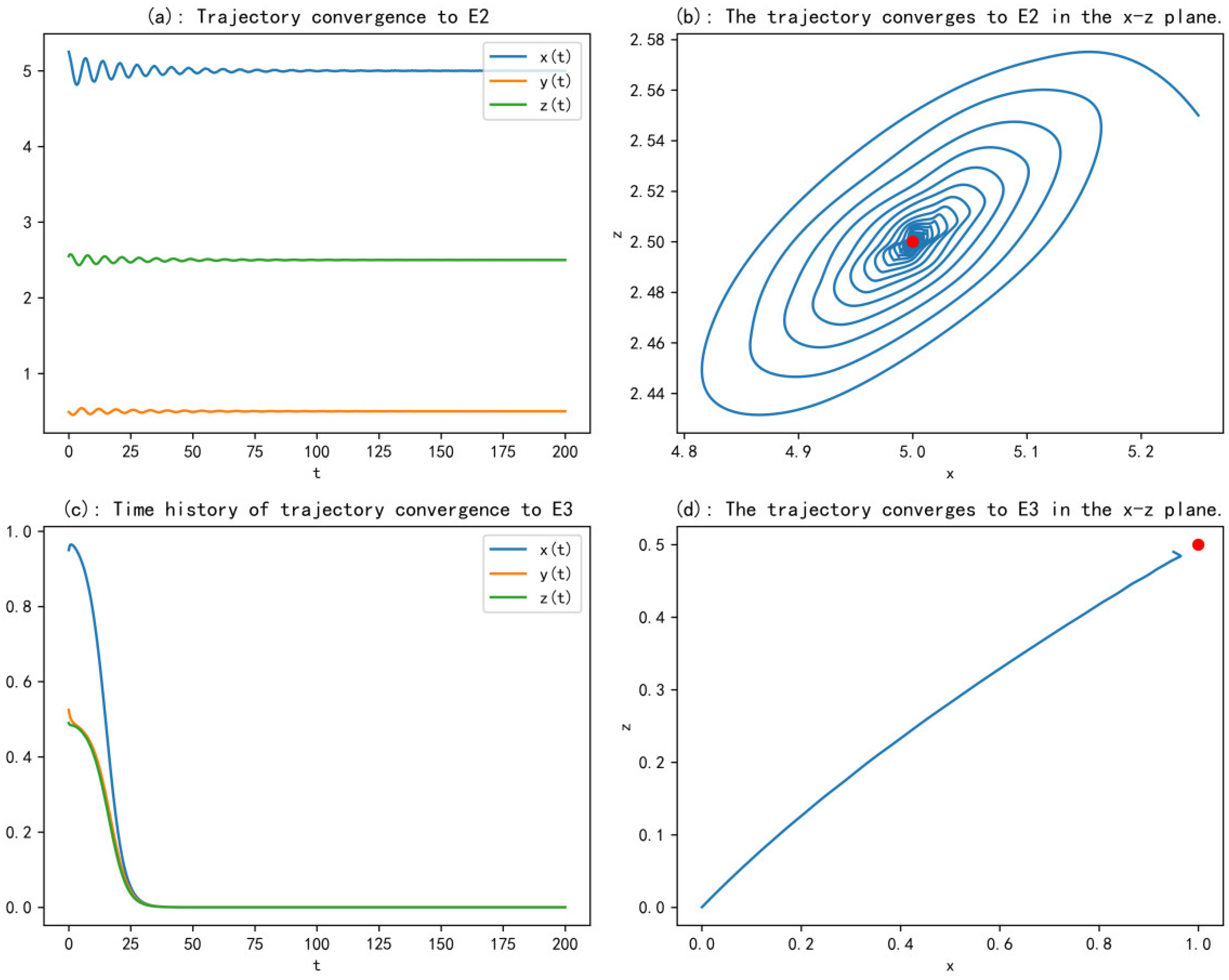
Using Firm A’s calibrated baseline parameters $a=b=c=1.0,\eta =0.2$, and $\delta =0.5$, we set the learning efficiency to $\alpha =0.6$ (as in Figure 2). By Theorem 1, the system has three equilibria: $E_1=(0,0,0),E_2=(5,0.5,2.5),E_3=(1,0.5,0.5).$ We then evaluate the Jacobian matrix at each equilibrium and compute its eigenvalues. The results are consistent with the analytical stability conditions. For E1, all eigenvalues are negative. This is expected under $ac>\delta$. Here $ac=1$ and $\delta =0.5$. The origin is therefore locally asymptotically stable under the baseline parameters. For E2, the eigenvalues all have negative real parts. E2 is locally asymptotically stable. For E3, at least one eigenvalue is positive. E3 is unstable (a saddle). These numerical results match the stability classification derived earlier.

Figure 2 visualizes these stability properties in the time domain and in phase space. In Figure 2a, we perturb the initial condition slightly around E2. The trajectories of $x\left(t\right)$, $y\left(t\right)$, and $z\left(t\right)$ show damped oscillations and converge to $E_2=\left(5,0.5,2.5\right)$. This indicates local attraction around the high-innovation equilibrium. Figure 2b plots the trajectory in the $x-z$ plane. The spiral path converges to the equilibrium marked by the red point. In contrast, Figure 2c,d correspond to the neighborhood of E3. Although $E_3=\left(1,0.5,0.5\right)$ is a nonzero equilibrium, it is a saddle under the baseline parameters. Trajectories initiated near E3 do not generally converge to it. The phase portrait shows divergence away from the equilibrium along an unstable direction. Taken together, these simulations imply that, under Firm A’s current parameter configuration, the long-run dynamics are primarily governed by E1 and E2. In this setting, E2 corresponds to a stable operating regime with high innovation, moderate absorptive capacity, and relatively strong performance.

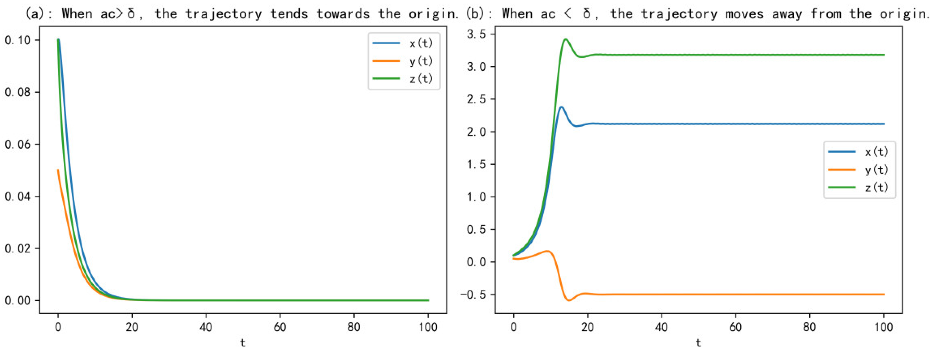
Figure 3 provides an additional trajectory-based check of Theorem 2 on the stability of the origin $E_1=(0,0,0)$. In Figure 3a, we keep Firm A’s baseline parameters and impose $ac>\delta$ (here $a=c=1,\delta =0.5$, so $ac=1>\delta$). Starting from a small perturbation $\left(x_0,y_0,z_0\right)=\left(0.1,0.05,0.1\right)$, all three state variables decay monotonically to zero. The origin is locally attractive. This corresponds to a self-reinforcing “low innovation–low capability–low performance” regime. In Figure 3b, we construct a contrast case by increasing $\delta$ so that $ac<\delta$ (e.g., $\delta =1.5$, hence $ac=1<1.5$). Under the same initial condition, the trajectory no longer returns to the origin. It departs rapidly and approaches a new level. Both $x\left(t\right)$ and $z\left(t\right)$ rise and stabilize at positive values, while $y\left(t\right)$ drops below zero. The negative $y\left(t\right)$ does not imply a negative capability in practice. It reflects the normalization scale of the model. It indicates that the organization’s carrying capacity is insufficient relative to the speed of innovation–performance reinforcement, producing an “capacity gap/organizational overload” configuration. Overall, Figure 3 shows in a transparent way that the inequality $ac\gtrless \delta$ determines the local stability of the origin, and it provides a numerical basis for the subsequent discussion of multistability and bifurcation behavior.

These results suggest that the equilibria identified in the model correspond to distinct organizational states in digital transformation. The origin (E1) represents a low-activity regime in which innovation efforts fail to accumulate into capability and the firm remains at a low level of transformation. The high-level equilibrium (E2) represents a stable transformation regime in which innovation, capability accumulation, and performance reinforcement are aligned. The intermediate equilibrium (E3) acts as a threshold-like state separating these regimes. In organizational terms, this implies that firms are not continuously improving along a single path; rather, they tend to operate within relatively stable regimes unless key conditions shift.

5.2. Dynamics with $\alpha$ as the Bifurcation Parameter

Under Firm A’s baseline calibration ($a=b=c=1.0,\eta =0.2,\delta =0.5$), we have $ac=1.0>\delta =0.5$. In this parameter setting, changes in the learning-efficiency parameter $\alpha$ alter the existence of equilibria, their local stability, and the long-run behavior of the system. To align with the regime classification in Theorem 5, we hold $a,b,c,\eta ,\delta$ fixed at their calibrated values and treat $\alpha$ as the sole control parameter.

The saddle-node threshold is obtained from the discriminant condition $\Delta =a^2-0.2$. This yields ${\alpha }_{SN}\approx 0.4472$. When $\alpha >{\alpha }_{SN}$, the two nonzero equilibria E2 and E3 exist. We then compute the Hopf boundary numerically. The results identify a Hopf point for E2 at ${\alpha }_{H2}\approx 0.6390$. This value marks a qualitative change in the dynamics. For $\alpha <{\alpha }_{H_2}$, trajectories near E2 converge to the equilibrium. For $\alpha >{\alpha }_{H_2}$, trajectories no longer converge to E2. A persistent periodic oscillation emerges, i.e., a limit cycle.

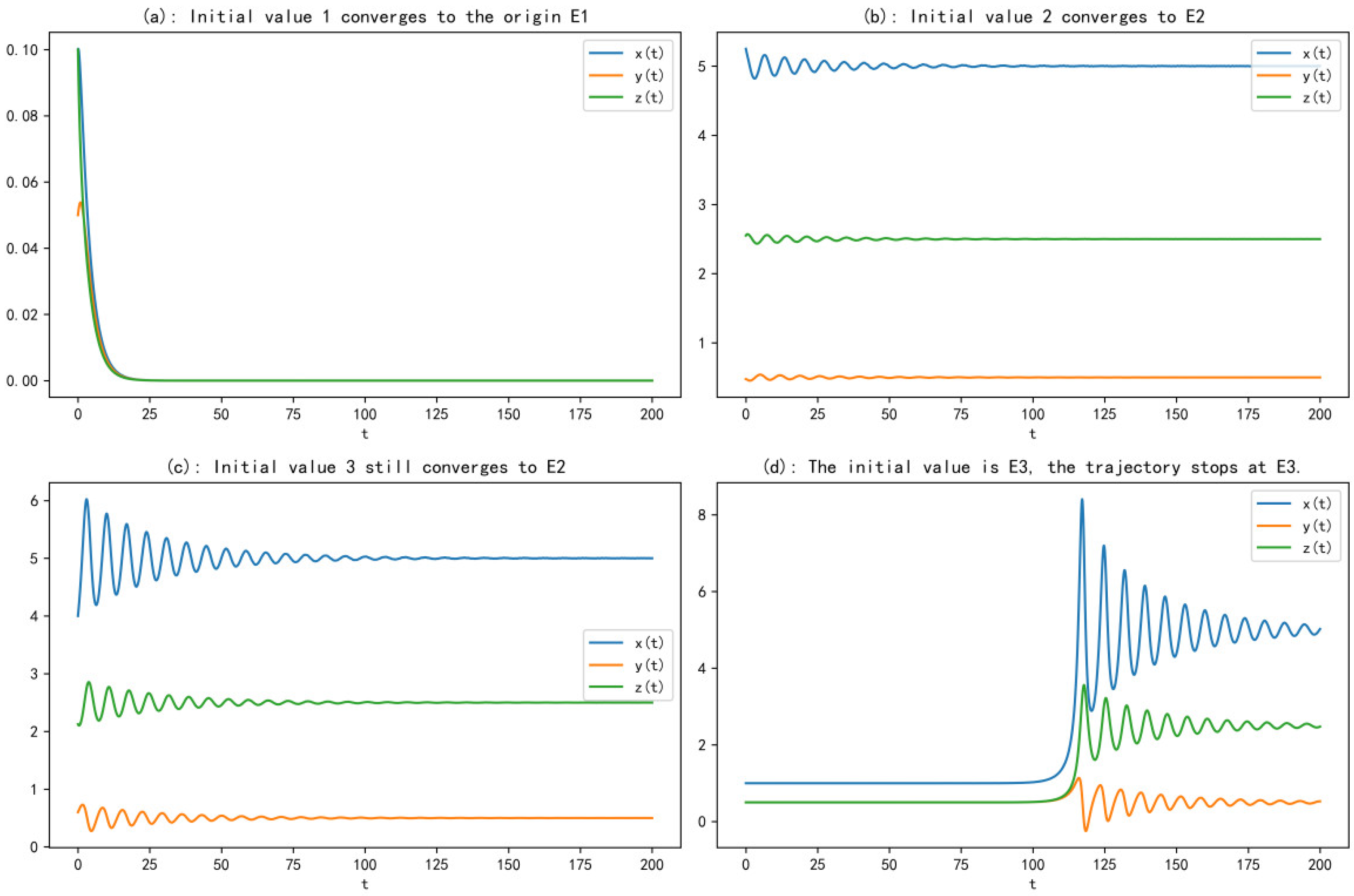
Figure 4 links long-run outcomes to initial conditions under the same structural parameters and the same $\alpha$. In Figure 4a, we choose a small perturbation near the origin, $\left(x_0,y_0,z_0\right)=\left(0.10,0.05,0.10\right)$. All three state variables decay rapidly and converge to E1. The origin is attractive under this calibrated configuration. Figure 4b,c use two “high-level” initial states, selected in the neighborhood of E2 or slightly displaced from it. In both cases, $x\left(t\right)$, $y\left(t\right)$, and $z\left(t\right)$ exhibit damped oscillations and converge to the same nonzero equilibrium, $E_2=\left(5.0,0.5,2.5\right)$. This indicates that E2 is a stable attractor with a nontrivial basin. Figure 4d starts from the nonzero equilibrium $E_3=\left(1.0,0.5,0.5\right)$. Both the theoretical classification and the numerical eigenvalue results indicate that E3 is a saddle under the baseline parameters. It is not attractive. Small perturbations can drive the trajectory away from E3 and toward another attractor. In simulations, this appears as a long residence near E3 followed by a drift and eventual convergence to a different stable state. Figure 4 therefore illustrates a clear form of initial-condition dependence. The system can fall into a low-level lock-in state (convergence to E1) or move into a high-innovation steady state (convergence to E2). E3 behaves as a threshold-type equilibrium rather than a long-run destination.

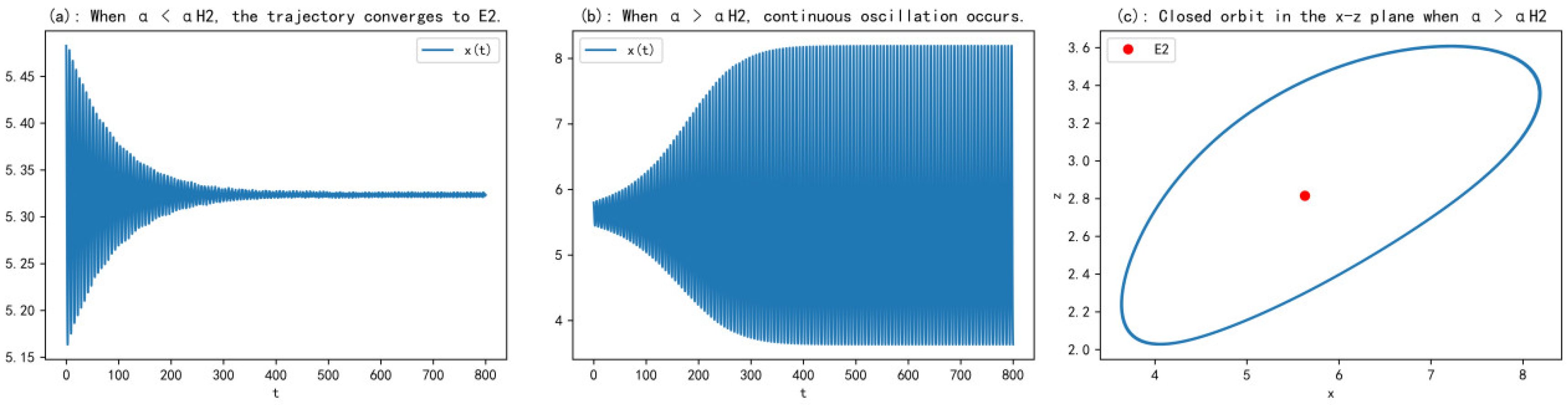
Figure 5 examines directly how the stability of E2 changes when $\alpha$ is the control variable. Figure 5a reports the case $\alpha <{\alpha }_{H_2}$. The state variable $x\left(t\right)$ shows damped oscillations and converges to a constant level. This is consistent with complex eigenvalues whose real parts are negative. Figure 5b reports $\alpha$ slightly above ${\alpha }_{H_2}$. The oscillations no longer decay. The trajectory settles into a periodic motion with a stable amplitude. This indicates that E2 has lost local stability and that a limit cycle has emerged. Figure 5c plots the closed orbit in the $x–z$ plane. The red marker denotes the location of E2. The closed orbit provides a direct geometric signature of the Hopf bifurcation. The long-run regime shifts from a steady state to a periodic operating mode. In managerial terms, once learning efficiency exceeds a threshold, innovation effort, absorption, and performance feedback can generate endogenous oscillations. The observed pattern is “advance–adjust–advance,” not convergence to a fixed level.

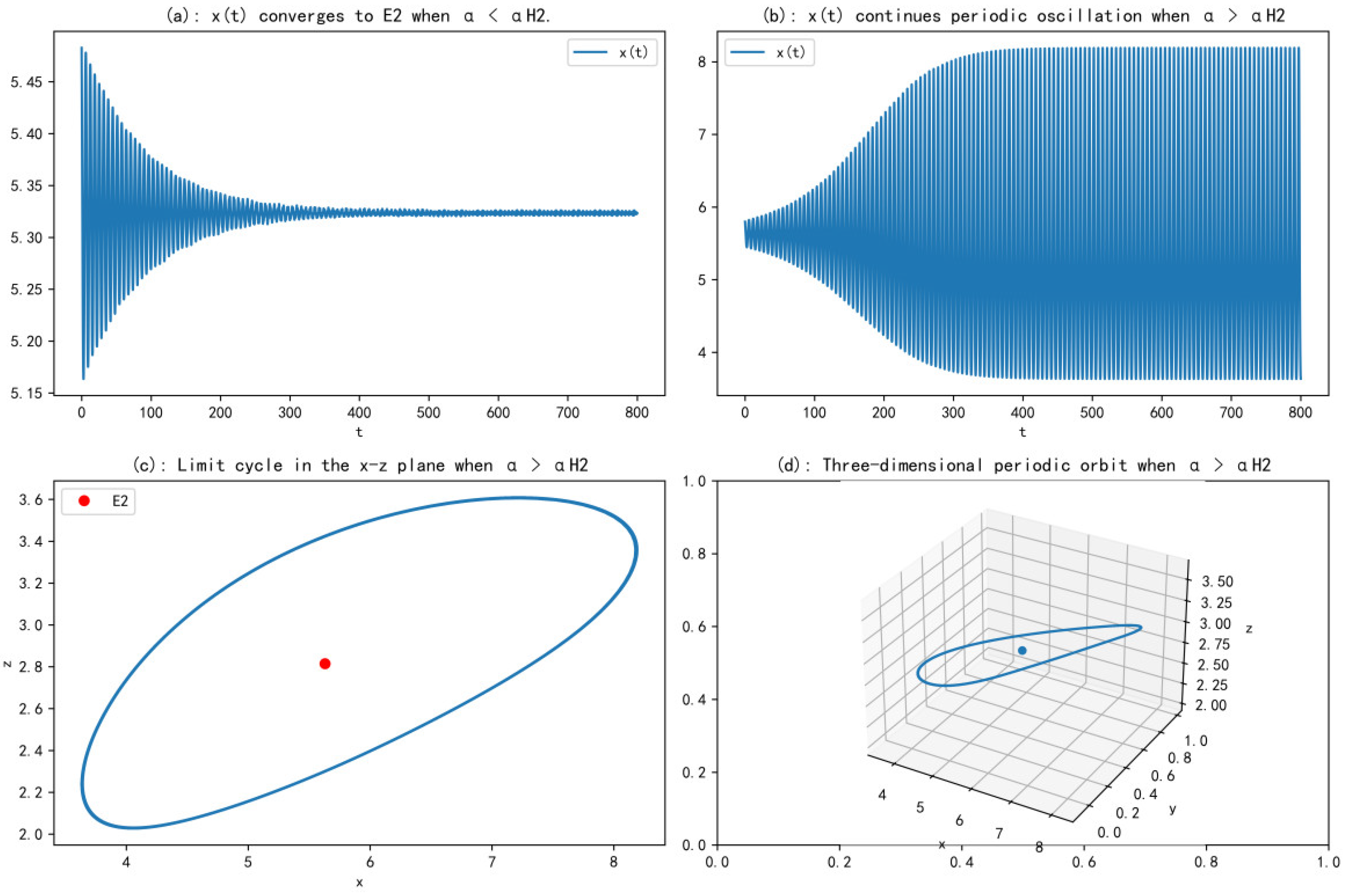
Figure 6 provides additional evidence for the post-Hopf periodic attractor. Figure 6a,b compare $x\left(t\right)$ under $\alpha >{\alpha }_{H_2}$. The former shows damped convergence. The latter shows sustained periodic oscillation with a stable amplitude after a transient phase. Figure 6c again shows a clear closed loop in the $x–z$ plane, with E2 marked for reference. Figure 6d plots the trajectory in three-dimensional phase space $\left(x,y,z\right)$. The trajectory forms a closed curve. This rules out an artifact created by two-dimensional projection. In other words, when $\alpha$ crosses ${\alpha }_{H_2}$, the system transitions from a point attractor to a periodic attractor, and the periodic behavior is synchronized across all three state variables. The amplitude and frequency of these oscillations can be examined further in subsequent analyses of amplitude–parameter and period–parameter relationships.

The bifurcation thresholds identified in the model can be interpreted as organizational tipping points rather than directly observable parameters. For example, the saddle-node threshold (${\alpha }_{SN}$) represents the minimum level of learning efficiency required for a firm to sustain a non-zero transformation trajectory. In practice, this corresponds to the point at which experience from digital initiatives begins to accumulate into stable organizational capability. Similarly, the Hopf threshold (${\alpha }_H$) marks the transition from stable improvement to oscillatory behavior, which can be interpreted as the point at which coordination demands begin to exceed the organization’s capacity to manage simultaneous initiatives.

Although these thresholds are not directly observable, firms can infer their position relative to them through observable patterns. A firm operating below the first threshold is likely to experience repeated pilot efforts without sustained improvement. A firm near the threshold may show temporary gains that are not maintained. A firm beyond the threshold may achieve sustained improvement, but if it moves further into the high-efficiency region without sufficient coordination capacity, it may begin to exhibit cyclical patterns such as repeated expansion and retrenchment. In this sense, the thresholds provide a way to interpret observed transformation trajectories rather than precise numerical targets.

5.3. Bifurcation Diagram and Long-Run Behavior

In this subsection we vary the learning-efficiency parameter over $\alpha \in [0.2,1.2]$. We keep the baseline parameters fixed at $a=b=c=1.0,\eta =0.2$ and $\delta =0.5$. The discriminant condition $\Delta ={\alpha }^2-0.2$ yields the saddle-node threshold ${\alpha }_{SN}\approx 0.4472$. Solving the Hopf condition numerically gives ${\alpha }_{H_2}\approx 0.6390$. When $\alpha \ge {\alpha }_{SN}$, the nonzero equilibrium branches exist and admit closed-form expressions: $x_2(\alpha )={\displaystyle \frac{\alpha +\sqrt{{\alpha }^2-0.2}}{0.2}}$, $x_3(\alpha )={\displaystyle \frac{\alpha -\sqrt{{\alpha }^2-0.2}}{0.2}}$. At $\alpha ={\alpha }_{SN}$, the two branches coincide, $x_2=x_3\approx 2.2361$. At $\alpha ={\alpha }_{H2}$, we obtain $x_2\approx 5.4745,x_3\approx 0.91552$.

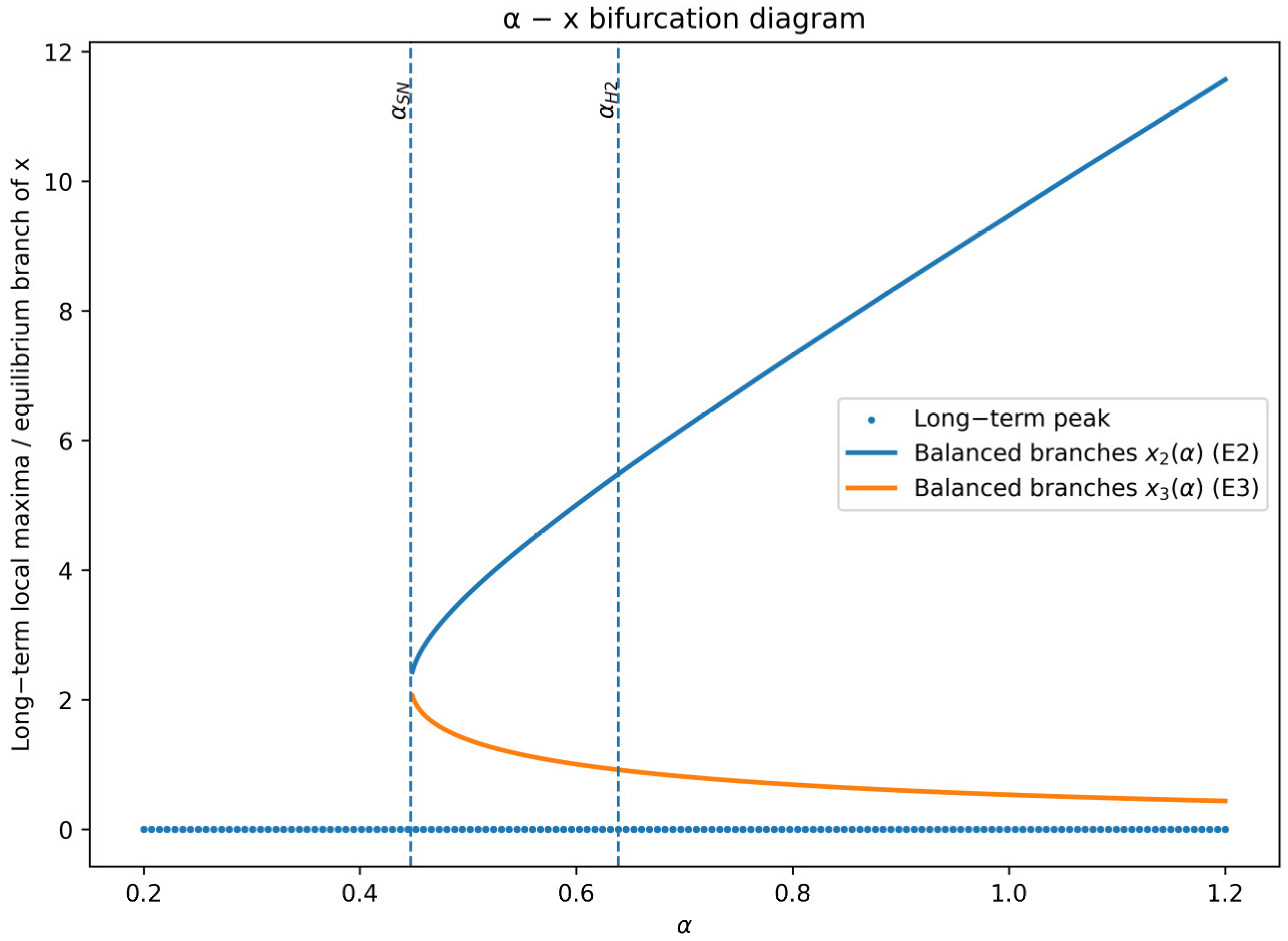
Figure 7 summarizes the sequence “branch emergence–stability change–long-run attainability.” For $\alpha <{\alpha }_{SN}$, only the origin branch exists. When $\alpha$ crosses ${\alpha }_{SN}$, the nonzero equilibria split into a high branch $x_2(\alpha )$ and a low branch $x_3(\alpha )$. The high branch increases with $\alpha$. The low branch decreases with $\alpha$. This pattern implies that stronger learning efficiency pushes the high-innovation steady state to a higher level. The vertical marker at ${\alpha }_{H_2}$ indicates the Hopf boundary around E2. For $\alpha >{\alpha }_{H_2}$, a stable periodic orbit appears in the neighborhood of E2. The long-run behavior changes from point convergence to sustained oscillation. The diagram also highlights an important distinction. Most simulated long-run peak points remain close to zero under the current setup. This means that many initial conditions fall inside the basin of attraction of the origin E1. The system then returns to the low-level lock-in regime. This observation does not contradict the existence of a limit cycle for $\alpha >{\alpha }_{H_2}$. It reflects basin geometry. The branch can exist, but it may not be reached. Only when the initial state enters the attraction basin of E2 do the long-run peaks on the right side of ${\alpha }_{H_2}$ display the typical “vertical spread” associated with periodic bifurcation.

5.4. Robustness and Sensitivity Analysis

To assess the robustness of the model results, we conduct a one-at-a-time sensitivity analysis based on Firm A’s calibrated parameters.

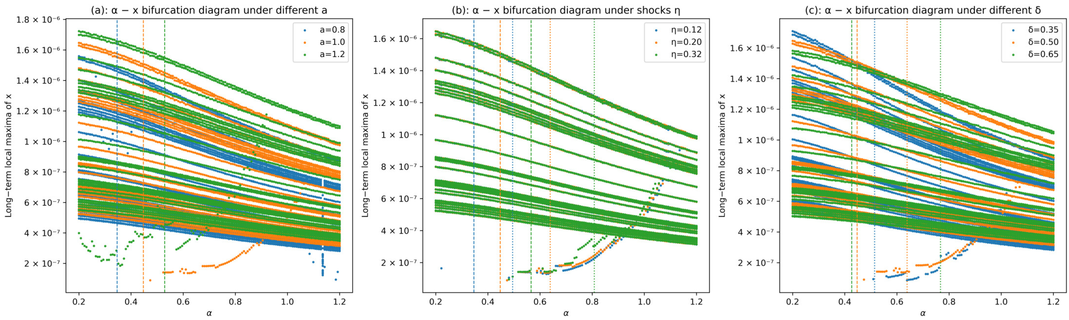
Figure 8 reports a one-at-a-time sensitivity analysis calibrated to Firm A. Unless otherwise stated, the baseline parameter set is $a=1, b=1, c=1, \eta =0.2, \delta =0.5$. For each panel, only one structural parameter is perturbed while the remaining parameters are held at their baseline values. The bifurcation parameter $\alpha$ is scanned over [0.2, 1.2]. The vertical dashed lines indicate the critical value at which non-zero operating regimes become admissible under the corresponding parameter setting.

Figure 8a varies the organisational threshold $a$ with $a\in \left\{0.8,1.0,1.2\right\}$. As a increases, the critical α shifts rightward, implying a higher learning efficiency is required for the system to depart from the low-level state and sustain a non-zero regime. Moreover, the range of α over which the high-activity branch is practically attainable becomes narrower, consistent with stronger organisational “entry barriers” dampening the feasibility of persistent high-innovation operation. Figure 8b varies the complexity shock $\eta$ with $\eta \in \{0.12,0.2,0.32\}$ Larger $\eta$ not only increases the critical $\alpha$ but also brings forward the onset of oscillatory responses, indicating that heightened coordination frictions compress the stable operating region and make cyclical adjustment more likely. Figure 8c varies the conversion efficiency $\delta$ with $\delta \in \{0.35,0.5,0.65\}$. Higher $\delta$ generally reduces the learning-efficiency requirement for reaching a non-zero regime, but it may simultaneously enlarge the amplitude of endogenous fluctuations once the system enters the post-critical region, reflecting an amplification of feedback when performance responds strongly to innovation inputs.

Taken together, Figure 8 suggests lower organisational thresholds (smaller $a$) and weaker complexity frictions (smaller $\eta$) facilitate earlier entry into sustained non-zero operation and widen the stable region. Improvements in conversion efficiency (larger $\delta$) help translate innovation into performance at lower levels of learning efficiency, but such gains are most sustainable when accompanied by measures that limit coordination frictions and strengthen organisational capacity, otherwise the system is more prone to persistent oscillations. These results suggest that while parameter changes affect the location of thresholds and stability regions, the core dynamic patterns identified in the model remain qualitatively robust.

6. Discussion and Managerial Implications

The preceding analysis identifies several possible dynamic patterns of digital transformation, including low-level persistence, stable improvement, and recurrent fluctuation. Before deriving managerial implications, it is necessary to clarify the scope and limits of these results. The model offers a mechanism-based explanation of divergent transformation trajectories, but it does not provide an exhaustive account of all organizational and environmental factors that may affect digital transformation outcomes.

6.1. Critical Discussion: Limitations, Alternative Explanations, and Boundary Conditions

While the numerical results support the proposed dynamic interpretation of digital transformation, the model should not be read as a complete explanation of all transformation outcomes. It intentionally focuses on three core state variables: technological innovation intensity, absorptive capacity, and operational performance. This parsimonious structure helps clarify the feedback mechanisms among innovation effort, learning accumulation, and performance, but it necessarily excludes other factors that may also shape transformation trajectories. For example, leadership commitment, organizational culture, resource slack, external competition, regulatory pressure, vendor dependence, and technological maturity may influence whether digital transformation stabilizes, stalls, or fluctuates over time. These factors are not denied by the model, but they are outside the current analytical boundary.

Alternative explanations should therefore be acknowledged. Divergent transformation outcomes may arise not only from differences in absorptive capacity or coordination complexity, but also from differences in market demand, financial constraints, industry maturity, institutional environments, or external shocks. For example, unstable performance may reflect disruptions in demand, supply chains, or regulation rather than internal coordination pressure alone. Similarly, sustained performance improvement may reflect favorable market growth, stronger resource endowments, or managerial intervention, rather than capability accumulation alone. The model therefore provides a mechanism-based explanation of divergent outcomes, but it should not be interpreted as an exhaustive account or as ruling out other organizational and environmental explanations.

These considerations also define the boundary conditions of the model. The model is most applicable to firms in which digital transformation unfolds through multiple interdependent initiatives and where innovation activities, learning processes, and operational performance can be observed over time. It is particularly relevant to manufacturing and operations-intensive contexts, where digital initiatives affect production routines, data governance, delivery capability, and cross-functional coordination. By contrast, the model may be less applicable to settings where digital transformation is driven by a single discrete technology adoption, where performance is dominated by external market shocks, or where organizational learning is difficult to retain across projects. It may also have limited explanatory power in highly turbulent environments where exogenous disturbances overwhelm internal feedback mechanisms.

These limitations clarify rather than weaken the contribution of the model. The purpose of the model is not to provide a universal explanation of digital transformation, nor to establish empirically identified causal effects. Instead, it specifies one theoretically grounded mechanism through which similar digital transformation efforts may produce different long-run trajectories. By making the model’s assumptions, alternative explanations, and boundary conditions explicit, the analysis offers a more cautious and robust interpretation of digital transformation dynamics.

6.2. Managerial Implications

Subject to these boundary conditions, the model offers several managerial implications for firms seeking to sustain digital transformation over time.

(1)

Increasing technological innovation intensity does not guarantee performance improvement

The results suggest that increasing technological innovation intensity does not automatically lead to improvements in operational performance. Under similar conditions, firms may follow different trajectories, including sustained improvement, persistence at a low level, or repeated fluctuation. This indicates that increasing investment or accelerating implementation alone may not ensure effective transformation. For managers, “doing more” or “moving faster” should therefore not be treated as sufficient strategies. Even when innovation activities continue to expand, a lack of stable performance improvement may indicate that the current transformation path is not producing effective results.

In practice, firms should establish performance evaluation cycles for each round of digital initiatives, focusing on whether performance improves in a sustained manner rather than whether projects are completed on schedule. Before launching new initiatives, managers should assess whether existing projects have generated stable performance gains. If consecutive initiatives fail to produce sustained improvement, further expansion should be paused and attention redirected toward identifying underlying problems. In this sense, evaluation should shift from the number of completed projects to the trajectory of performance outcomes.

(2)

The key issue is not only investment level, but whether absorptive capacity is formed

The findings indicate that technological innovation intensity contributes to operational performance only when it is translated into absorptive capacity. When experience generated from innovation activities is absorbed and retained, performance improvement becomes more likely to persist. In contrast, when such experience is fragmented or lost, performance may remain at a low level despite continuous investment. Therefore, the central managerial issue is not simply whether innovation activities are continuously pursued, but whether they are transformed into cumulative organizational capability.

Accordingly, firms should establish structured processes to ensure that experience from each initiative is captured and reused. After each project, organizations should identify which aspects of experience can be transferred and how they will be applied in subsequent initiatives. New projects should build on previously accumulated experience rather than start from scratch. If experience is not carried across projects, expansion should be slowed and priority should be given to strengthening capability accumulation. In this sense, the reuse of experience should be treated as a key indicator of whether absorptive capacity is being developed.

(3)

Parallel innovation activities may increase coordination pressure and weaken performance improvement

The results further suggest that as technological innovation intensity increases, the number of parallel activities may also rise, leading to greater coordination pressure. When coordination capacity does not improve accordingly, the positive effect of absorptive capacity on operational performance may weaken, and performance may become less stable. This implies that during expansion, increasing coordination demands can undermine sustained improvement and lead to repeated adjustment.

From a managerial perspective, the number of concurrent initiatives should be actively controlled. Firms should set clear limits on the number of projects running simultaneously and assess whether the current level of activity exceeds the organization’s coordination capacity. Before launching new initiatives, managers should evaluate how many projects are already underway and whether additional activities can be effectively coordinated. When signs such as frequent project adjustments, inconsistent outcomes across initiatives, or repeated disruptions emerge, expansion should be slowed. A deceleration mechanism should be established so that new projects can be paused when coordination pressure becomes excessive or when performance begins to fluctuate, allowing existing initiatives to stabilize.

(4)

Transformation outcomes depend on the alignment among innovation intensity, absorptive capacity, and coordination constraints

The study suggests that digital transformation outcomes are not determined by a single factor, but by the interaction among technological innovation intensity, absorptive capacity, and coordination constraints. Under different conditions, firms may remain at a low level, achieve sustained improvement, or enter fluctuating states. This implies that similar levels of investment can lead to different outcomes depending on how innovation effort, capability accumulation, and coordination pressure evolve together.

Therefore, decisions to expand innovation intensity should be based on the alignment between organizational capability and coordination conditions. Before increasing the scale of innovation activities, firms should assess three key aspects: whether experience from previous initiatives has been retained and reused, whether operational performance shows sustained improvement rather than temporary gains, and whether current activities remain stable without excessive coordination strain. Only when these conditions are sufficiently met should further expansion be pursued. If any of these conditions is not met, expansion should be paused and efforts redirected toward strengthening internal capability and coordination. In this sense, sustainable digital transformation depends not only on the speed of expansion, but also on maintaining alignment between innovation intensity, capability accumulation, and coordination capacity.

7. Conclusions

This study examines how technological innovation intensity shapes the long-run performance of digital transformation within firms. Although many firms continue to expand digital initiatives, their outcomes do not necessarily converge. Some firms are able to build organizational capability and sustain improvement, while others remain in low-level adjustment or experience unstable performance over time.

To account for these differences, the study develops a nonlinear dynamic model that links technological innovation intensity, absorptive capacity, and operational performance. The model further incorporates experience accumulation, coordination constraints, and performance feedback. Numerical analyses are then used to examine how these relationships evolve under different organizational conditions, and an embedded case study is introduced to compare the model’s implications with observed implementation patterns.

Three conclusions follow. First, digital transformation should not be understood as a simple process in which stronger innovation effort leads directly to better performance. Firms facing similar external conditions may still arrive at different long-run outcomes, including persistent low-level operation, sustained improvement, or continuing fluctuation. Second, the effect of technological innovation intensity depends on whether experience from innovation activities is retained and translated into absorptive capacity. Where this process is weak, firms may continue to increase innovation effort without building lasting capability. Where it is sufficiently strong, sustained performance improvement becomes possible. Third, performance becomes less stable when innovation activities expand faster than the organization’s ability to coordinate them. As parallel initiatives increase, coordination demands rise; if governance does not adjust accordingly, performance may weaken and repeated adjustment may become more likely.

Taken together, these findings show that the long-run results of digital transformation are not determined by technological innovation intensity alone. They depend on whether firms can turn innovation activity into accumulated capability and whether that process remains manageable as coordination demands increase. The study therefore contributes to the literature by offering a mechanism-based explanation of why similar digital transformation efforts may produce different outcomes over time.

Theoretically, this study links dynamic capabilities, organizational learning, and complexity theory in a unified explanation of digital transformation. It shows that resource reconfiguration through technological innovation is insufficient unless innovation experience is accumulated into absorptive capacity. It further shows that even when learning occurs, increasing coordination complexity may destabilize the transformation process and generate divergent long-run trajectories. In this way, the study contributes not only a dynamic modeling approach, but also a theoretical account of how resource reconfiguration, learning accumulation, and coordination complexity jointly shape digital transformation outcomes.

This study has several limitations. The embedded case reflects a single organizational setting, and broader empirical evidence is therefore needed. Since the study relies on a theory-driven dynamic model and case-based calibration, the results should be interpreted as mechanism-based explanations rather than empirically identified causal effects. Some key constructs, particularly absorptive capacity and coordination quality, cannot be observed directly and remain difficult to measure with precision. Moreover, the model focuses mainly on internal dynamic mechanisms and does not fully incorporate alternative explanations such as leadership commitment, organizational culture, market conditions, institutional pressures, or external shocks. Future research could compare firms across industries and maturity levels, incorporate external uncertainty, and model managerial decisions, such as portfolio selection and pacing, more explicitly. These extensions would further clarify when digital transformation stabilizes and when it remains uneven.