Optimization of Transportation and Delivery Routes Under Regional Constraints: A Two-Stage Solution Model Based on SDVRP and Truck-Drone Collaboration

Abstract

With the rapid development of e-commerce and the increasing complexity of urban logistics, traditional delivery methods face significant challenges due to regional traffic restrictions and congestion. This paper presents a two-stage optimization approach for urban delivery routing, integrating the Split Delivery Vehicle Routing Problem (SDVRP) and truck-drone collaboration to address these challenges. In the first stage, a transportation route optimization model based on SDVRP is proposed, which accounts for regional constraints and vehicle capacity limitations. The model allows for demand splitting, reducing the number of vehicles required and minimizing transportation costs. In the second stage, a truck-drone collaborative delivery model is introduced to handle the “last mile” distribution, where drones complement trucks by delivering to areas with restricted vehicle access. The optimization model aims to minimize overall delivery costs while ensuring timely service. An enhanced genetic algorithm is further developed to solve this complex, multi-constrained model. Experimental results show that the proposed collaborative strategy reduces delivery costs by over 10% compared to truck-only delivery, and the improved algorithm achieves a 4.77% average cost reduction over traditional approaches. This study provides valuable insights for optimizing urban logistics systems under regional constraints, offering both theoretical and practical contributions to smart logistics development.

1. Introduction

In recent years, the logistics industry has experienced rapid growth, accompanied by a continuous rise in transportation demand. Effective transportation route planning has become crucial for improving efficiency, reducing costs, and optimizing resource use. Optimized vehicle route planning enables enterprises to streamline logistics processes, minimize costs, and enhance overall operational efficiency. The Vehicle Routing Problem [1] is a well-known issue in operations research, focusing on planning vehicle routes from one or more origins (e.g., warehouses) to multiple destinations, subject to specific constraints. The core idea involves using mathematical models and optimization algorithms to identify the optimal transportation route, considering factors like customer demand, costs, and time constraints.

As transportation demand diversifies, particularly with accelerated urbanization and expanding product variety, transportation tools are constantly evolving, making the Multi-type Vehicle Routing Problem (MVRP) an increasingly prominent research topic. MVRP accounts for various vehicle types, including small trucks, large trucks, and refrigerated trucks, each differing in load capacity, speed, and suitable routes. Therefore, effectively coordinating their operations is crucial for route planning. Common MVRP models typically focus on two key aspects: (a) Vehicle collaboration, which is central to MVRP. Different vehicle types offer distinct advantages [2]. The challenge lies in integrating these characteristics with transportation needs to form an efficient model, which is crucial for optimization. For instance, large trucks may be assigned to long-distance transportation, while small trucks handle local deliveries within the city. With proper scheduling and collaboration, different vehicle types can complement one another’s strengths, optimizing route planning. (b) Tasking and resource scheduling, in multi-vehicle routing, task allocation and resource scheduling play a critical role. The model allocates tasks based on each vehicle’s transport capacity and route adaptability, ensuring timely and appropriate task completion.

In practical applications, multi-type vehicle collaborative transportation often encounters region-specific restrictions, with each vehicle type assigned a designated operational area, structured hierarchically [3]. For instance, transportation tools such as large trucks, small trucks, and drones face varying regional limitations. Large trucks typically handle long-distance transportation from central warehouses to regional sub-warehouses, with their operational areas being macro, mainly confined to highways and city outskirts. In contrast, small trucks are ideal for medium to short-distance deliveries and can access narrow areas such as cities or streets, performing deliveries from sub-warehouses to end users. Drones represent an innovative delivery method [4], capable of flying over cities or accessing hard-to-reach areas like mountains and islands, offering finer regional adaptability. Hence, it is clear that the regional restrictions of these vehicles create a hierarchical structure from macro to micro, requiring route planning to allocate tasks accordingly. Traditional multi-vehicle transportation methods often fail to address the hierarchical and differential nature of regional restrictions effectively, highlighting the urgent need for new methods to solve these practical issues.

The main challenges in addressing the multi-vehicle transportation problem with regional restrictions are as follows. First, determining how to allocate transportation tasks and routes efficiently at each level to optimize overall transportation efficiency and cost. For instance, in the collaboration between large and small trucks, minimizing costs while adhering to regional restrictions is a critical issue. Secondly, under varying regional restrictions, efficiently transferring tasks between different vehicle types is another pressing issue. Typically, large trucks manage long-distance transportation from the warehouse to sub-warehouses, while small trucks and drones handle “last-mile” deliveries from sub-warehouses to end users. When transferring tasks between transportation tools, especially between small trucks and drones, it is crucial to consider each vehicle type’s characteristics and the task’s urgency to avoid delays or additional transportation costs during transitions.

To tackle the aforementioned challenges, this paper proposes an innovative solution. First, this paper presents a multi-level regional division model to optimize transportation efficiency at each stage by effectively allocating tasks (e.g., from warehouse to sub-warehouse and from sub-warehouse to end users). Specifically, during long-distance transportation with large trucks, cost savings are realized by increasing load capacity and minimizing vehicle usage; in the last-mile phase, the collaborative delivery routes of small trucks and drones are optimized to ensure efficiency. Secondly, to resolve the transfer issue between vehicle types, particularly between vehicles and drones, this paper employs dynamic transfer, facilitating efficient task handover during delivery and minimizing delays caused by waiting for transfer. Additionally, this paper proposes an enhanced genetic algorithm optimization solution, which can effectively address the vehicle scheduling optimization problem across different regions. The innovations of this paper include (a) A multi-stage route optimization model that considers regional restrictions; (b) The use of dynamic transfer to address the transfer problem between vehicle types; (c) An improved traditional genetic algorithm to enhance the efficiency of solving transportation route and task allocation.

While a bi-level programming framework could theoretically consider the hierarchical nature of this problem, solving such a model with equilibrium constraints is computationally challenging for real-world scales. Therefore, we propose a computationally efficient two-stage solution model with a novel cost-driven coupling mechanism. This approach retains the essential interdependence of the two levels—the first-stage transportation plan is optimized with the knowledge of its impact on the second-stage costs—through an iterative reallocation process, offering a practical and effective alternative to a full bi-level formulation.

The rest of the paper is organized as follows. An overview of related academic literature is provided in Section 2. Section 3 gives the problem description and modeling. Section 4 provides the design improvement of the solution algorithm for this model. Section 5 provides some examples to verify the rationality of the model and algorithm in this paper. Finally, Section 6 gives some conclusions.

2. Literature Review

Since its inception in the 1950s, the Vehicle Routing Problem (VRP) has remained a fundamental challenge in the field of logistics optimization. The increasing diversification of logistical demands, coupled with the emergence of advanced technologies—most notably unmanned aerial vehicles (UAVs)—has given rise to a broad spectrum of VRP variants. This review provides a critical examination of the literature most pertinent to the proposed two-stage truck–drone collaborative model under regional constraints. Rather than offering an exhaustive enumeration of existing studies, we develop a focused narrative that traces the evolution from foundational ground-based routing models to contemporary aerial–ground coordination frameworks. The primary objective is to identify and explicitly articulate the research gaps that the present study aims to address.

2.1. The Foundation: Classical VRP and the Split Delivery Paradigm

The classical Vehicle Routing Problem (VRP), initially formalized by Dantzig and Ramser [1], has since evolved into a wide array of variants incorporating realistic operational constraints such as vehicle capacity, time windows, and multi-depot configurations [5,6]. A fundamental assumption underlying these classical formulations is the indivisibility of customer demand—i.e., each customer must be served by exactly one vehicle. While this assumption simplifies the modeling and solution process, it often leads to suboptimal resource utilization, particularly in contexts where individual customer demands constitute a substantial proportion of vehicle capacity.

To address this limitation, Dror and Trudeau [7] introduced the Split Delivery Vehicle Routing Problem (SDVRP), which relaxes the single-visit constraint by permitting a customer’s demand to be fulfilled through multiple vehicle trips. Their seminal work demonstrated that allowing split deliveries can substantially reduce both the number of vehicles employed and the total distance traveled—especially when individual customer demands exceed 10% of vehicle capacity. These findings have been corroborated by subsequent studies [8], positioning the SDVRP as a critical modeling paradigm for high-demand or capacity-constrained logistics environments.

The practical relevance of the Split Delivery Vehicle Routing Problem (SDVRP) has been substantiated across a variety of application domains, including maritime logistics [9], helicopter scheduling [10], livestock feed distribution [11], and disaster relief operations [12]. In parallel, solution methodologies have advanced considerably—progressing from exact algorithms [13,14,15,16] to heuristic and metaheuristic approaches capable of addressing large-scale, real-world instances [17,18,19].

Despite its demonstrated efficacy in improving routing efficiency, the SDVRP framework—like its classical predecessors—remains constrained by a fundamental assumption: fleet homogeneity. Specifically, existing SDVRP models uniformly assume that all vehicles are identical in terms of capacity, operational characteristics, and—critically—access permissions. This assumption fails to consider the operational complexity of contemporary urban logistics environments, where vehicle types differ not only in capacity and cost but also in their ability to navigate heterogeneous urban zones subject to differential access restrictions. For instance, large trucks, smaller delivery vans, and unmanned aerial vehicles (UAVs) operate in fundamentally distinct spatial and regulatory domains—a reality that homogeneous fleet models are inherently ill-equipped to address.

In parallel, recent advances in evolutionary algorithms have addressed large-scale CVRP instances. Zheng et al. [20] proposed an evolutionary multiobjective route grouping-based heuristic, decomposing problems by routes rather than customers—a strategy conceptually similar to the split delivery paradigm

2.2. Toward Heterogeneity and Hierarchy: Multi-Echelon Routing

The recognition that real-world logistics operations employ diverse vehicle types led to the development of the Heterogeneous Vehicle Routing Problem (HVRP), introduced by Golden et al. [21]. HVRP and its extensions (with time windows, pickup and delivery, etc.) acknowledge that vehicles differ in capacity, operating costs, and performance characteristics. However, these models remain grounded in a single-echelon perspective: all vehicles operate from the same distribution center and serve customers directly.

A more structurally significant advancement in the evolution of routing models is the formalization of the Two-Echelon Vehicle Routing Problem (2E-VRP), introduced by Perboli and Tadei [3]. This framework introduces a hierarchical logistics structure that more accurately reflects the operational realities of urban distribution networks. In the 2E-VRP, first-echelon vehicles—typically large trucks—transport goods from a central depot to intermediate facilities (e.g., satellites, urban consolidation centers, or warehouses). Subsequently, second-echelon vehicles execute the last-mile delivery to end customers. This tiered spatial configuration naturally accommodates differential access restrictions prevalent in urban environments, where large trucks may be barred from city centers while smaller, more agile vehicles can navigate deeper into densely populated areas.

The foundational 2E-VRP model has been significantly enriched by subsequent research. Hemmelmayr et al. [22] developed adaptive large neighborhood search algorithms specifically tailored to city logistics contexts. Enthoven et al. [23] extended the model by integrating coverage-based options, enabling second-echelon vehicles to serve customers either directly or via intermediate points such as parcel lockers. Dellaert et al. [24] incorporated time windows and proposed exact solution methodologies. Exact methods for two-echelon problems have also been advanced. Liu et al. [25] developed a branch-and-cut algorithm for the two-echelon capacitated vehicle routing problem with grouping constraints, while Song et al. [26] derived improved lower bounds for the adaptive version. Sitek et al. [27] proposed a multi-agent approach for multi-echelon VRPs, and Raidl et al. [28] applied logic-based Benders decomposition to a bi-level CVRP. Santos et al. [29] introduced a branch-and-cut-and-price algorithm for the 2E-CVRP. More recently, the growing electrification of urban fleets has prompted the integration of electric vehicles into the second echelon [30,31,32].

Despite these advancements, existing 2E-VRP formulations exhibit two critical limitations when applied to the context of modern aerial–ground logistics systems.

First, the second echelon in conventional 2E-VRP remains exclusively ground-based. Intermediate facilities are serviced by surface vehicles—such as electric vans, cargo bikes, or couriers—rather than by aerial platforms with fundamentally different operational characteristics. Drones introduce a distinct set of constraints, including three-dimensional movement, flight endurance limitations, no-fly zones, and line-of-sight requirements, all of which lie beyond the scope of traditional ground-based routing models. Although recent studies by Li et al. [33] and Zhou et al. [34] have proposed two-echeleon frameworks incorporating drones, such contributions remain exceptional rather than representative of the broader literature.

Second, and more fundamentally, the concept of synchronization in 2E-VRP differs qualitatively from that required in truck–drone collaborative systems. In standard two-echelon models, synchronization refers primarily to temporal coordination—ensuring that goods are available at intermediate facilities prior to last-mile dispatch. In contrast, truck–drone systems demand both temporal and spatial synchronization, as drones must rendezvous with trucks at precise locations and times to facilitate battery swapping, payload transfer, or coordinated operations. For a comprehensive overview of two-echelon vehicle routing problems, readers are referred to the recent survey by Sluijk et al. [35]. This represents a substantially more complex coordination problem, one for which conventional two-echelon formulations are inherently ill-suited.

Recent evolutionary algorithm developments have addressed heterogeneous and hierarchical routing contexts. Wang et al. [36] developed a multifidelity-based ant colony optimization for electric vehicle routing, balancing computational efficiency with solution accuracy. More relevant to our two-stage framework, Jiang et al. [37] proposed a surrogate-assisted bi-level evolutionary algorithm for multi-depot vehicle routing with uncertain demand, where upper-level facility decisions and lower-level routing are coupled through machine learning approximations—a paradigm that parallels our cost-driven coupling mechanism

2.3. Aerial-Ground Coordination: Truck-Drone Collaborative Delivery

The advent of unmanned aerial vehicles (UAVs) as viable platforms for last-mile delivery has catalyzed a distinct and rapidly expanding body of research focused on the unique challenges associated with aerial–ground coordination. This section provides a critical examination of the relevant literature, with particular emphasis on synchronization mechanisms and the modeling of operational constraints inherent to hybrid truck–drone systems. Beyond commercial parcel delivery, drones have been deployed in humanitarian logistics, such as healthcare services for chronic disease patients in rural areas [38], emergency blood supply [39], and medical item delivery in urban settings [40].

2.3.1. Synchronization Mechanisms: From Single-Echelon to Two-Echelon Coordination

The truck–drone collaborative delivery problem was first systematically formalized by Murray and Chu [41] through the introduction of the Flying Sidekick Traveling Salesman Problem (FSTSP). In this foundational model, a single truck functions as a mobile depot, launching and recovering a single drone at designated rendezvous points. The synchronization mechanism is sequential and location-fixed: the drone is launched from a truck location, serves exactly one customer, and returns to the same truck at a predetermined rendezvous point. While innovative, this mechanism imposes significant operational constraints—the truck must remain stationary during drone operations, and each drone flight is limited to a single customer per sortie.

In response to these limitations, subsequent research progressively relaxed these initial assumptions. Murray and Raj [4] extended the model to accommodate multiple drones (mTSP-D), enabling parallel operations in which several drones could be launched simultaneously. Raj and Murray [42] extended the multiple flying sidekicks model to incorporate variable drone speeds, demonstrating that speed adjustments can significantly reduce delivery time under time-sensitive conditions. Boccia et al. [43] further proposed a column-and-row generation approach for the flying sidekick traveling salesman problem, achieving exact solutions for moderately sized instances. Sacramento et al. [44] developed an adaptive large neighborhood search heuristic for the vehicle routing problem with drones (VRPD), facilitating implicit coordination between multiple trucks and drones. Kitjacharoenchai et al. [45] proposed a variant allowing multiple drone deliveries per trip, introducing per-trip synchronization whereby drones execute multi-stop routes before returning to the truck.

More recent contributions have explored increasingly sophisticated synchronization mechanisms. Poikonen and Golden [46] formalized the trade-offs between launch frequency and drone range limitations. Agatz et al. [47] provided a comprehensive optimization framework for the traveling salesman problem with drone, comparing exact and heuristic approaches. Yurek and Ozmutlu [48] proposed a decomposition-based iterative optimization algorithm for the TSP with drone, achieving efficient solutions for larger instances. Roberti and Ruthmair [49] developed exact solution methods capable of solving small-scale instances. Zhou et al. [34] proposed branch-and-price algorithms that explicitly handle synchronization constraints for instances involving up to 35 customers.

Critical assessment and identification of Gap 1: Despite the progressive relaxation of modeling assumptions, the existing literature on truck–drone synchronization exhibits a persistent and significant gap: all current models operate within a single-echelon paradigm, wherein trucks serve as mobile depots operating directly from a central distribution center. The problem of two-echelon synchronization—in which first-echelon trucks transport goods to intermediate warehouses or urban consolidation centers, and second-echelon truck–drone teams subsequently operate from those facilities—has been entirely overlooked.

This distinction is not merely taxonomic; it introduces qualitatively different coordination challenges. In single-echelon models, synchronization is primarily spatial in nature, focusing on the selection of rendezvous locations. In contrast, two-echelon systems require spatio-temporal synchronization characterized by cascading dependencies: the start time of second-echelon operations is contingent upon first-echelon arrival times, and delays propagate across echelons. To date, no study has addressed this multi-level synchronization challenge. This gap is fundamental and directly motivates the two-stage architectural framework proposed in the present study. A comparative study of operational modes for coordinated last-mile deliveries with trucks and drones was recently conducted by Ding et al. [50], highlighting the trade-offs between launch frequency and route efficiency.

2.3.2. Regional Constraints in Truck-Drone Systems

Critical assessment and identification of Gap 2: In the domain of urban logistics, regional constraints manifest as heterogeneous access restrictions that differentially affect vehicle types based on their operational characteristics. Large trucks may be entirely prohibited from city centers, smaller trucks may be subject to time-of-day access limitations, and drones face a distinct set of spatial constraints including no-fly zones, altitude ceilings, and mandatory proximity buffers relative to infrastructure. Despite the practical salience of such restrictions, their treatment in the existing literature remains fragmented and conceptually underdeveloped.

She et al. [51] examined the impact of low-altitude traffic congestion on drone routing, demonstrating that airspace density significantly influences delivery performance. More recently, ElSayed and Mohamed [52] provided the first systematic investigation of how regulatory stringency—encompassing parameters such as maximum allowable altitude and required horizontal separation from buildings—affects drone energy consumption. Their findings reveal that stricter regulations can increase energy demand by up to 400% in dense urban environments, underscoring that regional constraints influence not only route feasibility but also operational costs in ways that transcend binary access permissions.

Despite these isolated contributions, existing truck–drone routing models either omit regional constraints altogether or represent them as simplistic binary restrictions. A unified hierarchical framework that captures type-specific access permissions across nested spatial domains—wherein large trucks, small delivery vehicles, and drones operate within progressively finer-grained zones subject to differentiated regulatory regimes—remains absent from the literature. This gap is particularly consequential for urban logistics applications, where access regulations are inherently hierarchical and vehicle-type-specific. Addressing this lacuna is essential for developing routing models that reflect the operational realities of contemporary multimodal urban delivery systems.

2.3.3. A Parallel Literature: UAV Energy Consumption Modeling

Parallel to the development of routing optimization models, a distinct and growing body of literature has focused on the fundamental physics underlying UAV energy consumption. Importantly, this research stream has evolved largely independently of truck–drone routing studies—a disciplinary separation that presents significant limitations for operational modeling, given that energy constraints are central to drone feasibility in real-world applications.

Kunarak [53] decomposes total UAV energy expenditure into mechanical and communication-related components, demonstrating that consumption is critically influenced by flight altitude, velocity, and payload mass—factors uniformly abstracted away in routing models that rely on static endurance assumptions. ElSayed and Mohamed further show that regulatory constraints, such as altitude limits and building proximity requirements, can increase energy demand by up to 400% in dense urban settings, a finding with profound implications for route planning under realistic operational conditions. Kierzkowski et al. [54] provide empirical validation for fixed-wing UAVs, revealing that turning maneuvers incur substantial energy penalties and that actual consumption exceeds theoretical estimates by approximately 30%. Collectively, these findings suggest that routing models predicated on simplified distance- or time-based endurance thresholds may systematically underestimate true energy requirements, thereby compromising solution feasibility in practice.

Critical assessment and identification of Gap 3: Despite the maturity and relevance of the energy-aware UAV literature, truck–drone routing research continues to rely on simplistic static constraints—typically expressed as maximum flight distance or flight time—that fail to capture the dynamic and context-sensitive nature of energy consumption. The integration of physics-based energy models into two-echelon routing frameworks remains an open and largely unaddressed research challenge.

We explicitly acknowledge that the present study, while directly addressing Gaps 1 and 2 through the formulation of a two-stage truck–drone collaborative model under regional constraints, retains a simplified static endurance representation. Accordingly, we identify the incorporation of dynamic, physics-informed energy models as a critical direction for future research. This acknowledgment situates our contribution within a broader research agenda while transparently delimiting its scope.

For dynamic environments requiring rapid adaptation, Liu et al. [55] introduced a data-driven evolutionary algorithm for vehicle routing with time windows under limited computational time, leveraging historical patterns to guide search. While focused on ground-based operations, their approach to handling time constraints could inform extensions of truck-drone collaborative models to dynamic urban logistics.

2.4. Synthesis: Articulating the Research Gap and Positioning This Study

The foregoing critical analysis reveals that the literature, as shown in

Table 1. Comparative Analysis of Representative Studies.

Study	Echelon Structure	Vehicle Types	Regional Constraint Handling
Single-Echelon Truck-Drone Collaboration
Murray & Raj [41]	Single-echelon	One truck + multiple drones	Not considered
Sacramento et al. [44]	Single-echelon	Multiple trucks + multiple drones	Not considered
Poikonen & Golden [46]	Single-echelon	Mothership + multiple drones	Not considered
Traditional Two-Echelon VRP (Ground Only)
Perboli & Tadei [3]	Two-echelon	Trucks	Not considered
Hemmelmayr [22]	Two-echelon	Trucks	Not considered
Dellaert [24]	Two-echelon	Trucks	Not considered
Two-Echelon Truck-Drone Collaboration
Kitjacharoenchai et al. [45]	Two-echelon	Trucks (1st) + Drones (2nd)	Not considered
Zhou et al. [34]	Two-echelon	Trucks + drones	Not considered
Studies with Regional Constraints
She R et al. [51]	Single-echelon	Trucks + drones	Airspace congestion
ElSayed [52]	Regulatory impact	Single-echelon	Regulatory strictness
Kunarak [53]	UAV-EMS	Single-echelon	Not considered
Kierzkowski et al. [54]	Holding maneuver	Single-echelon	Low-altitude constraints
This study	Two-echelon	Trucks (1st) + Drones (2nd)	Regional constraints

, despite its breadth and depth, has developed along parallel yet disconnected trajectories, with limited integration across key thematic areas. Three interconnected research gaps emerge with clarity:

Gap 1: Two-Echelon Synchronization. Existing truck–drone routing models operate exclusively within a single-echelon paradigm, wherein trucks function as mobile depots operating directly from a central distribution center. The problem of synchronizing first-echelon truck deliveries to intermediate warehouses with second-echelon truck–drone last-mile operations—a coordination challenge requiring both temporal alignment and spatial rendezvous under cascading time dependencies—has not been addressed in the literature.

Gap 2: Consider Regional Constraints. Current models treat regional access restrictions as binary, isolated, and vehicle-agnostic. A unified framework capable of capturing the hierarchical structure of real-world urban regulations—wherein large trucks, small delivery vehicles, and drones operate within nested spatial domains subject to type-specific access permissions—remains absent.

Gap 3: Energy-Conscious Routing. The truck–drone routing literature continues to rely on simplistic static endurance constraints (e.g., maximum flight distance or time), largely disregarding advances in UAV energy physics that demonstrate consumption is dynamically influenced by flight altitude, velocity, payload, and regulatory context.

This study directly addresses Gaps 1 and 2 by proposing an integrated modeling and optimization framework for two-echelon truck–drone routing under regional constraints. Specifically, we contribute: (i) a two-stage model incorporating explicit multi-level synchronization, wherein the first stage solves a Split Delivery Vehicle Routing Problem (SDVRP) for cross-regional truck transportation, and the second stage optimizes truck–drone last-mile operations, with the two stages coupled through demand propagation and time-coordination constraints; (ii) a regional constraint framework that operationalizes type-specific access zones across nested spatial domains, reflecting the regulatory heterogeneity of urban environments; and (iii) while Gap 3 lies beyond the scope of the present study, we explicitly identify its integration as a critical direction for future research, informed by the energy-aware UAV literature reviewed herein.

3. Problem Description and Model Formulation

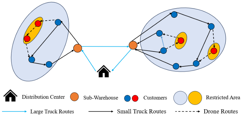
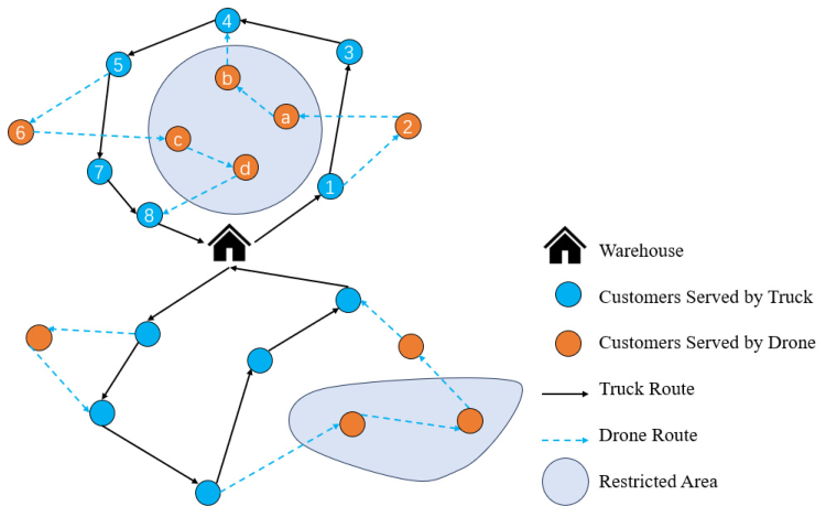
This section addresses the development of a vehicle routing optimization model under regional restriction policies. The problem involves three types of transportation vehicles: large trucks, small trucks, and drones. As shown in Figure 1, the distribution center plans to dispatch large trucks to transport goods and meet customer demand. However, due to restrictions on height, width, and weight, large trucks dispatched by the distribution center are prohibited from entering the light blue region in the figure. As a result, customers located in this restricted area cannot be directly serviced by large trucks. To resolve this issue, a warehouse-based approach is used, dividing the problem into two stages:

In the first stage, large trucks depart from the distribution center and deliver goods to warehouses located at the edge of the restricted area. In the second stage, a combination of small trucks and drones, permitted to enter the restricted zone, transports goods from the warehouse to the customers. In this phase, some customers may be difficult to reach due to management or other factors, as shown in the yellow region. For these customers, drones must be used for delivery to satisfy their needs.

The set of models, parameters, and decision variables are given in

Table 2. Sets, parameters, and decision variables of the model.

Sets
$C$	set of all customer nodes
$C^{\prime }\subset C$	set of customer nodes accessible by trucks (truck-accessible customers)
$O_0$	set of distribution centers (central depot)
$O$	set of sub-warehouses (intermediate facilities)
$V$	set of all nodes in Stage 1, $V=O_0\cup O$
$N$	set of all nodes in Stage 2, $N=C\cup O$
$R_d\subset N$	set of nodes where drones can depart from trucks (departure rendezvous points)
$R_a\subset N$	set of nodes where drones can return to trucks (arrival rendezvous points)
$R=R_d\cup R_a$	set of all possible rendezvous nodes
$N_{+}$	set of successor nodes (nodes that can be reached from a given node)
$N_{-}$	set of predecessor nodes (nodes from which a given node can be reached)
$K$	set of trucks (including both large trucks in Stage 1 and small trucks in Stage 2)
$D$	set of drones
$A$	set of all feasible arcs (directed connections between nodes)
$A_K\subset A$	set of arcs traversable by trucks
$A_D\subset A$	set of arcs traversable by drones
Parameters
$d_{ij}$	distance from node $i\in N$to node $j\in N$(applicable to all vehicle types)
$q_i$	demand (quantity of goods) required at customer node $i\in C$
$g_i$	total demand at node $i\in V$(used in Stage 1 for warehouse demand)
$L^K$	maximum payload capacity of a truck
$L^D$	maximum payload capacity of a drone
$C^K$	transportation cost per unit distance for trucks
$C^D$	transportation cost per unit distance for drones
$\left[T_i^e\right|T_i^l]$	time window for service at node $i\in N$; $T_i^e$is earliest start time, $T_i^l$is latest start time
${\tau }_{ij}^K$	travel time required for a truck to travel from node $i$to node $j$
${\tau }_{ij}^D$	travel time required for a drone to travel from node $i$to node $j$
$S_i^K$	service time of a truck at node $i\in N$
$S_i^D$	service time of a drone at node $i\in C$(drones do not service warehouses)
$T^D$	maximum allowable flight time per sortie for a drone (endurance limit)
$M$	a sufficiently large positive constant (big-M) used in logical constraints
Decision Variables
$x_{ij}^k$	binary variable, equals 1 if truck $k\in K$travels directly from node $i$to node $j$($i\ne j$), and 0 otherwise
$y_{ij}^d$	binary variable, equals 1 if drone $d\in D$travels directly from node $i$to node $j$($i\ne j$), and 0 otherwise
$w_{ki}$	continuous non-negative variable, quantity of goods delivered by vehicle (truck) $k$to node $i\in V$(used in Stage 1)
$w_i^k$	continuous non-negative variable, cumulative load of truck $k\in K$upon arrival at node $i\in N$(used in Stage 2)
$w_i^d$	continuous non-negative variable, cumulative load of drone $d\in D$upon arrival at node $i\in C$in a single sortie
$T_i^k$	continuous non-negative variable, arrival time of truck $k\in K$at node $i\in N$
$T_i^d$	continuous non-negative variable, arrival time of drone $d\in D$at node $i\in N$
$u_i^k$	continuous non-negative variable, waiting time of truck $k\in K$at node $i\in N$before commencing service or departure
$u_i^d$	continuous non-negative variable, waiting time of drone $d\in D$at node $i\in N$before commencing service or departure
$t_i^d$	continuous non-negative variable, cumulative flight time of drone $d\in D$since last departure from a truck in the current sortie, upon reaching node $i\in C$
$y_i^k$	binary variable (auxiliary), equals 1 if truck $k\in K$services node $i\in V$, and 0 otherwise (used in Stage 1)

.

3.1. The First Stage: Cross-Regional Transportation

In the first phase of this problem, vehicles are required to depart from the distribution center and deliver goods to multiple sub-warehouses in the city. To model this scenario, the Split Delivery Vehicle Routing Problem is employed. The SDVRP model was introduced into vehicle routing problems by Dror and Trudeau in 1989. The key distinction between SDVRP and the traditional Vehicle Routing Problem is that SDVRP allows a customer to be serviced by two or more vehicles. Compared to traditional VRP solutions, SDVRP can significantly reduce the number of delivery vehicles and shorten the overall route in many cases. This advantage becomes even more pronounced when the average demand of a customer exceeds 10% of the vehicle’s minimum capacity.

3.1.1. Properties of SDVRP

Due to the relaxed conditions of customer splitting in SDVRP, this model not only maximizes the payload of vehicles and reduces the number of vehicles required, but also effectively seeks shorter routes by satisfying the inequality constraints. The SDVRP model was first introduced by Dror and Trudeau [7], who demonstrated that allowing split deliveries can substantially reduce both the number of vehicles employed and the total distance traveled.

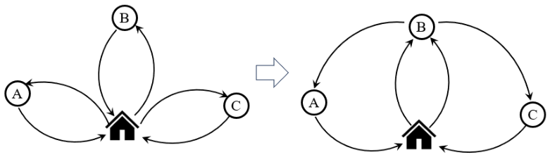
Consider a distribution center with three delivery points. The distances between the points, the customer demands, and the maximum vehicle capacity are nearly equal. The maximum capacity of each vehicle is 100, with the warehouse located at point O. The demands at points A, B, and C are 60 each. The delivery routes for both split and non-split deliveries are illustrated as shown in Figure 2:

Using the split delivery model in this dispatch scenario reduces the number of vehicles by one. When the inequality $\left|\mathrm{AB}\right|+\left|\mathrm{BC}\right|<\left|\mathrm{OA}\right|+\left|\mathrm{OC}\right|$ is satisfied, the total route distance for the split delivery is shorter than that for the non-split delivery.

3.1.2. Mathematical Model for Stage 1

The objective of Stage 1 is to minimize the total transportation cost (distance-based) of all large trucks while satisfying the demand requirements of all sub-warehouses. The model allows for split deliveries, meaning a sub-warehouse’s demand may be fulfilled by multiple truck visits.

The mathematical model for vehicle optimization scheduling is as follows:

$$\mathit{min}\hspace{0.33em}{Z}_1=\sum _{k\in K}\sum _{i\in N}\sum _{j\in N}{C}^K{d}_{ij}{x}_{ij}^k$$

(1)

$$\sum _{k\in K}{w}_{ki}=g_i,i\in O$$

(2)

$$w_{ki}\le g_i{y}_i^k,i,\in \mathrm{O},k\in K$$

(3)

$$\sum _{i\in O}{w}_{ki}\le {\mathrm{L}}^{\mathrm{K}},k\in K$$

(4)

$$\sum _j{x}_{ij}^k=\sum _j{x}_{ij}^k=y_k^i,i\ne j,i\in V,k\in K$$

(5)

$$\sum _{i\in S}\sum _{j\in S}{x}_{ij}^k\le \mid S\mid -1,\forall S\subset O,\mid S\mid \ge 2,\forall k\in K$$

(6)

$$x_{ij}^k\in \left\{\mathrm{0,1}\right\},i,j\in \mathrm{V},k\in K$$

(7)

$$y_i^k\in \left\{\mathrm{0,1}\right\},i,j\in V,k\in K$$

(8)

$$w_{ki}\ge 0,i\in \mathrm{O},k\in K$$

(9)

Constraint (2) ensures that the total quantity of goods delivered to sub-warehouse i by all trucks equals its demand $g_i$.

Constraint (3) links the delivery quantity variable $w_{ki}$ to the service indicator $y_i^k$. If truck k does not service warehouse i ($y_i^k=0$), then the delivered quantity must be zero. If it does service warehouse i ($y_i^k=1$), the delivered quantity cannot exceed the warehouse’s demand.

Constraint (4) is the truck capacity constraint: the total quantity delivered by truck k across all sub-warehouses it visits cannot exceed its maximum payload capacity $L^K$.

Constraint (5) enforces flow conservation. For any node i (including the distribution center and sub-warehouses), if truck k enters node i, it must also leave node i, unless i is the starting depot. This ensures route continuity. The equation also defines the relationship between the route variables $x_{ij}^k$ and the service indicator $y_i^k$. For the distribution center $O_0$, we have $y_{O_0}^k=1$ for all trucks that are used.

Constraint (6) eliminates subtours—i.e., closed loops that do not include the distribution center. This is a standard subtour elimination constraint for vehicle routing problems, ensuring that all routes start and end at the distribution center.

Constraints (7)–(9) define the domains of the decision variables.

Note on the minimum number of vehicles: The minimum number of trucks required for Stage 1 can be estimated as $\lceil {\displaystyle \frac{{\sum }_{i\in O}{g}_i}{L^K}}\rceil$. However, the actual number used is determined by the optimization process and may be higher due to routing constraints and time windows.

3.2. The Second Stage: Truck-Drone Collaborative Model

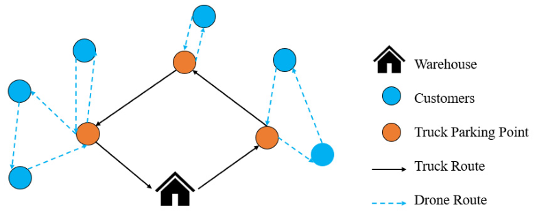
As depicted in Figure 3, the second stage of the model employs a truck-drone collaborative delivery system. The vehicle departs the warehouse with the drone and returns after completing the delivery task.

3.2.1. Regional Access Constraints

This study categorizes the limitations of the regions involved into two types. The first type, as introduced earlier in this chapter, results from restrictions on vehicle dimensions, such as height, width, and weight, which prevent large trucks from entering restricted areas. To resolve this issue, the study employs a method of establishing sub-warehouses and divides the problem into two stages.

We acknowledge that the current formulation represents regional constraints as a practical abstraction: access permissions are modeled as binary, and more complex conditions (e.g., no-fly zones, altitude limits, time-dependent access) are incorporated through parameterization (e.g., infinite travel costs on prohibited arcs, time window adjustments) rather than through explicit mathematical constraints. This abstraction is a deliberate choice to maintain computational tractability, but it does not constitute a fully explicit formulation of the full complexity of real-world airspace and regulatory conditions.

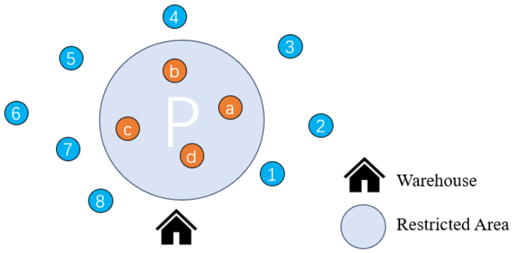
The second type of limitation applies within the second-stage delivery area. As shown in Figure 4, some customers (e.g., a, b, c, d) are located in zones where even small trucks are prohibited or cannot efficiently operate (e.g., pedestrian zones, narrow streets). These customers must be served exclusively by drones. To model this, we define the set $C^{\prime }\subset C$ as the set of customer nodes accessible by small trucks. Customers in $C\setminus C^{\prime }$ can only be served by drones.

Furthermore, the model is designed to be flexible in adapting to various real-world scenarios through parameter adjustments:

No-fly zones can be encoded during preprocessing by modifying the travel cost matrix—assigning infinite costs to drone arcs $y_{ij}^d$ that cross restricted airspace.

Altitude or energy constraints are reflected by adjusting the drone’s maximum flight time parameter $T^D$.

Time-dependent access restrictions (e.g., trucks prohibited during peak hours) can be enforced directly through the customer time window constraints $\left[T_i^e\right|T_i^l]$.

This design keeps the model focused on its primary objective—optimizing truck-drone collaborative routes—while maintaining adaptability to diverse real-world constraints through parameterization.

3.2.2. Truck-Drone Synchronization and Transshipment Constraints

Most existing studies on truck-supported drone delivery assume that trucks serve only as mobile warehouses during delivery tasks, without actively engaging in the delivery process [39]. As illustrated in Figure 5, the truck departs the warehouse, carrying both goods and a drone, and follows a predetermined route to various docking points. The drone then delivers the goods to customer points, while the truck remains stationary, functioning as a temporary warehouse. To enhance transportation efficiency and ensure full utilization of the truck, this model proposes the simultaneous use of both the truck and drone for delivery tasks. While the drone is performing deliveries, the truck can also engage in the delivery process, thus improving overall efficiency.

To enable collaborative delivery between the truck and drone, it is essential to ensure that both the truck and drone occupy the same location at the same time when the drone departs from and returns to the truck. Specifically, during the same time interval, both the truck and drone must be positioned at the same node. To achieve this, the starting times of the truck and drone are defined, ensuring that both delivery tasks can commence synchronously, thereby avoiding scheduling conflicts. The following constraints are introduced: (10) and (11):

$$T_0^k=0,\forall k\in K$$

(10)

$$T_0^d=0,\forall d\in D$$

(11)

To complete the delivery tasks within the specified time window, it is crucial to efficiently arrange the transshipment nodes for both the truck and drone. A time sequence is employed to record the arrival and departure times of both the truck and drone at each node. To optimize the scheduling of their departure times, parameters $u_i^k$ and $u_i^d$ are introduced, representing the waiting times for the truck and drone at node i, respectively. This approach also better accommodates the time window requirements for customer points. The following constraints are introduced: (12)–(14):

$$T_j^k\ge T_i^k+S_i^k+{\tau }_{ij}^k+u_i^k-M\left(1-x_{ij}^k\right),\forall k\in K,(i,j)\in A,j\in C^{\prime }$$

(12)

$$T_j^d\ge T_i^d+{\tau }_{ij}^D+u_i^d-M\left(1-y_{ij}^d\right),\forall d\in D,(i,j)\in A,i\in R_d$$

(13)

$$T_j^d\ge T_i^d+S_i^D+¦{\tau }_{ij}^D+u_i^d-M(1-y_{ij}^d),\forall d\in D,(i,j)\in A,i\notin R_d$$

(14)

In this model, the arrangement of transshipment between the truck and drone is critical. If the truck arrives at the transfer point after the drone, the drone may have no place to dock, causing the delivery task to fail. Therefore, it is essential to ensure that the truck arrives at the transfer point prior to the drone, facilitating a smooth transshipment process. The following constraints are introduced: (15) and (16):

The synchronization constraints can be expressed in corrected form as:

$$T_i^d\ge T_i^k+u_i^k-M\left(1-{\sum }_{j\in N_{+}}{y}_{ij}^d\right),\forall i\in R_d,d\in D,k=\mathit{associated} \mathit{truck}$$

(15)

$$T_j^d\ge T_j^k+u_j^k-M\left(1-{\sum }_{i{N}_{-}}{y}_{ij}^d\right),\forall j\in R_a,d\in D,k=\mathit{associated} \mathit{truck}$$

(16)

Constraint (15) ensures that if drone d departs from rendezvous point i (${\sum }_{\mathrm{j}}{\mathrm{y}}_{\mathrm{i}\mathrm{j}}^{\mathrm{d}}=1$), its departure time $T_i^d$ must be no earlier than the time the associated truck k is available at i ($T_i^k+u_i^k$). Constraint (16) similarly ensures that if drone d returns to rendezvous point j (${\sum }_i{y}_{ij}^d=1$), its arrival time $T_j^d$ must be no earlier than the truck’s available time at j. This guarantees that the drone never arrives before the truck, preventing failed rendezvous.

3.2.3. Drone Payload and Mileage Constraints

In this problem, the truck’s mileage constraint is not considered; however, the drone’s delivery task is limited by battery life. Excessive flight time can result in battery depletion, preventing the drone from completing the task. Therefore, the flight time constraint is critical for ensuring the smooth progress of the task. Cumulative flight time constraints are implemented to ensure that the duration of a single flight does not exceed the maximum allowable flight time. A limitation is set on the drone’s single flight duration to prevent the operating time from surpassing its maximum endurance. The following constraints are introduced: (17)–(19):

$$t_j^d\ge {\tau }_{ij}^D+M(y_{ij}^d-1),\forall d\in D,(i,j)\in A,i\in R_d$$

(17)

$$t_j^d\ge t_i^d+S_i^D+{\tau }_{ij}^D+M(y_{ij}^d-1),\forall d\in D,(i,j)\in A,i\notin R_d$$

(18)

$$t_i^d\le T^D,\forall d\in D,i\in C$$

(19)

Unlike the truck, where each unit is used only once in the delivery tasks, the drone can be used multiple times. Therefore, a maximum payload constraint must be imposed on each drone flight to ensure that the drone’s payload capacity does not exceed its design limit during the entire delivery process. The following constraints are introduced: (20)–(22):

$$w_i^d\le L^D,\forall d\in D,i\in C$$

(20)

$$w_j^d\ge q_j+M(y_{ij}^d-1),\forall d\in D,(i,j)\in A,i\in R_d,j\notin R_a$$

(21)

$$w_j^d\ge w_i^d+q_j+M(y_{ij}^d-1),\forall d\in D,(i,j)\in A,i\notin R_d,j\notin R_a$$

(22)

3.2.4. The Complete Model

The objective of this part of the model is to minimize the total transportation cost for the integrated truck and drone delivery system. Specifically, the objective function is composed of two components: the truck delivery cost and the drone delivery cost.

The objective function is as follows:

$$\mathit{min}\hspace{0.33em}Z=\sum _{k\in K}\sum _{(i,j)\in A}{C}^K{d}_{ij}{x}_{ij}^k+\sum _{d\in D}\sum _{(i,j)\in A}{C}^D{d}_{ij}{y}_{ij}^d$$

(23)

The specific constraints are as follows:

$$\sum _{j\in N_{+}}{x}_{o,j}^k\le 1,\forall k\in K$$

(24)

$$\sum _{i\in N_{-}}{x}_{i,c+1}^k\le 1,\forall k\in K$$

(25)

$$\sum _{k\in K}\sum _{i\in N_{-}}{x}_{ij}^k+\sum _{d\in D}\sum _{i\in N_{-}}{y}_{ij}^k=1,\forall j\in C$$

(26)

$$\sum _{i\in N_{-}}{x}_{ij}^k=\sum _{n\in N_{+}}{x}_{jn}^k,\forall k\in K,j\in C^{\prime }$$

(27)

$$\sum _{i\in N_{-}}{y}_{ij}^d=\sum _{n\in N_{+}}{y}_{jn}^k,\forall d\in D,j\in C$$

(28)

The truck-drone transshipment constraints are defined by Equations (10)–(16).

$$w_i^k\le L^K,\forall k\in K,i\in C$$

(29)

$$w_j^k\ge w_i^k+q_i+M\left(x_{ij}^k+y_{ij}^d-1\right),\forall k\in K,d=k,(i,j)\in A,j\in C$$

(30)

The drone’s payload and mileage constraints are defined by Equations (17)–(22).

$$T_i^e\le T_i^k\le T_i^l,\forall k\in K,i\in C^{\prime }$$

(31)

$$T_i^e\le T_i^d\le T_i^l,\forall d\in D,i\in C$$

(32)

$$x_{ij}^k,y_{ij}^d\in \left\{\mathrm{0,1}\right\}$$

(33)

$$u_i^k,u_i^d,T_i^k,T_i^d,t_i^d,w_i^k,w_i^d\ge 0$$

(34)

The objective function in Equation (23) represents the total cost of truck-drone delivery, with the first term accounting for the truck delivery cost and the second term for the drone delivery cost. Equations (24) and (25) ensure that each truck is used at most once. Equation (26) ensures that each consumer point is served exactly once. Equations (27) and (28) represent the continuity constraints for the movement of the truck and drone. The truck-drone transshipment constraints are defined by Equations (10)–(16). Equation (29) defines the truck’s maximum load capacity. Equation (30) represents the truck’s actual load. The drone’s payload and mileage constraints are defined by Equations (17)–(22). The start times for the truck and drone are defined by Equations (31) and (32), respectively. Equations (33) and (34) impose the variable constraints.

3.3. Two-Stage Coupling and Interaction Mechanism

3.3.1. Basic Interaction Mechanism

A critical aspect of the two-stage model is the interaction mechanism between stages, which ensures seamless coordination between the first-stage SDVRP and the second-stage truck-drone collaborative delivery. This interaction is established through two key coupling mechanisms: demand propagation and time coupling.

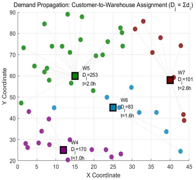
Demand Propagation. The demand at each sub-warehouse in the first stage is determined by the aggregated demands of customers assigned to that warehouse in the second stage. Let $C_j$ denote the set of customers assigned to sub-warehouse j. The demand $D_j$ at sub-warehouse j is calculated as: $D_j$= sum of d_i for all i in $C_j$. This ensures that the first-stage delivery quantities are dynamically determined by second-stage customer requirements.

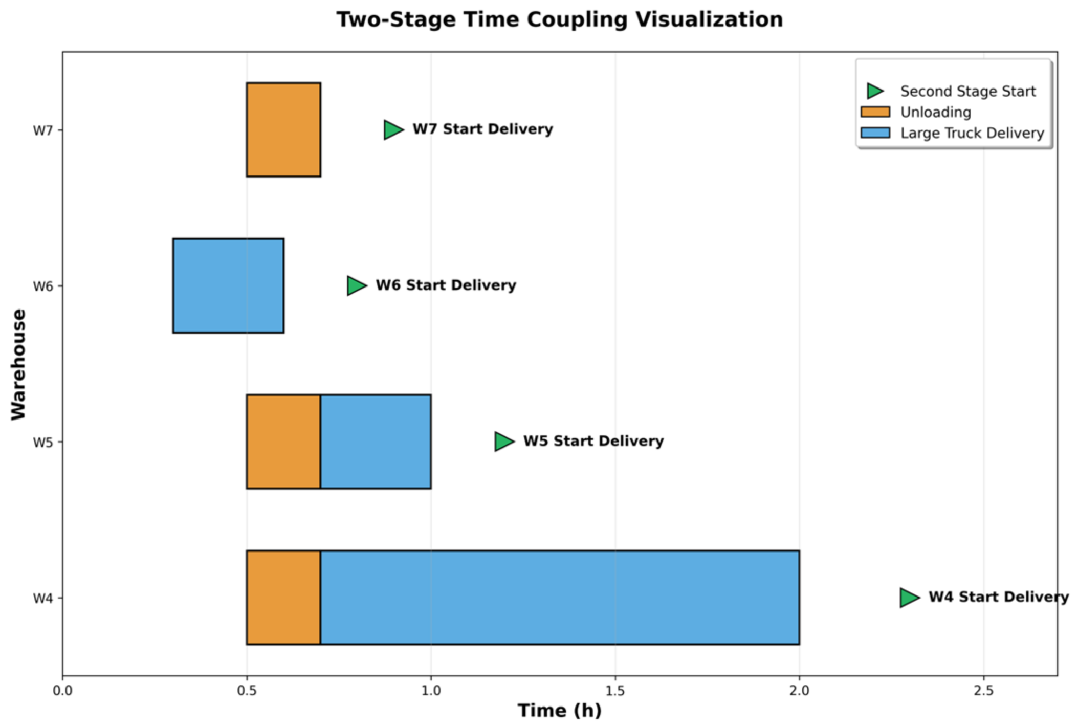
Time Coupling. The second stage cannot commence until the first stage completes delivery to the respective sub-warehouse. The time coupling constraint ensures temporal coordination, creating a unified timeline across both stages.

The two-stage coupling is mathematically formulated as follows. For demand propagation, the demand at sub-warehouse j is computed as:

$$D_j=SUM\left(d_i\right),foralliin{C}_j,foralljinW$$

(35)

where $C_j$ denotes the set of customers assigned to sub-warehouse j, $d_i$ is the demand of customer i, and W is the set of sub-warehouses. For time coupling, the start time of Stage 2 operations at warehouse j must satisfy:

$$t_j^{(S2,start)}>=t_j^{(S1,arrival)}+t^{\left(unload\right)},foralljinW$$

(36)

where $t_j^{(S1,arrival)}$ is the arrival time of the large truck at warehouse j in Stage 1, and t^(unload) is the unloading time. These constraints ensure that Stage 2 operations cannot begin until the goods have been delivered and unloaded from Stage 1.

Figure 6 and Figure 7 visualize these two interaction mechanisms. Figure 6 illustrates the demand propagation process, where customers are assigned to their nearest sub-warehouses. Figure 7 presents the time coupling between stages.

3.3.2. Cost-Driven Coupling and Customer Reallocation

While demand propagation and time coupling ensure operational feasibility, they do not guarantee optimality. The assignment of customers to warehouses—which directly determines the demand $D_j$ at each sub-warehouse—is not predefined and must be optimized to minimize the total system cost. To address this, we propose a cost-driven coupling mechanism that dynamically adjusts customer assignments based on the combined cost feedback from both stages.

Problem Description

Consider a multi-warehouse system with $M$ sub-warehouses $W=\{\mathrm{1,2},...,M\}$ and $N$ customers $C=\{\mathrm{1,2},...,N\}$. Each customer i has demand $q_i$ and a service cost $L_{ij}$ when assigned to warehouse j. The initial assignment follows the nearest distance principle: customer i is assigned to the warehouse with minimum $L_{ij}$.

The optimization objective is to achieve balance across all warehouses in terms of both load and cost through iterative customer reallocation, while ensuring that customers can only be transferred between adjacent warehouses—a constraint that reflects real-world logistics where customers are typically reassigned to nearby facilities.

Adjacent Warehouse Constraint

Define an adjacency matrix $Ad{j}_{M\times M}$ where

$Adj(p,q)=1$ if warehouse p and q are geographically adjacent (e.g., share service area boundaries, within a distance threshold, or connected by direct transportation links)

$Adj(p,q)=0$ otherwise

Customers can only be transferred between adjacent warehouses, ensuring that reallocation remains practically feasible.

Warehouse Performance Metrics

For each warehouse $j\in W$:

Total load:

$$T_j=\sum _{i\in C_j}{q}_i$$

(37)

Total cost:

$$C_j=\sum _{i\in C_j}{L}_{ij}$$

(38)

Identifying Imbalanced Warehouse Pairs

The set of all possible transfer pairs is restricted to adjacent warehouses:

$$P=\left\{\right(p,q)\mid Adj(p,q)=1\}$$

(39)

For each adjacent pair $(p,q)\in P$, calculate the cost imbalance ratio:

$$R_{pq}={\displaystyle \frac{\mathrm{m}\mathrm{a}\mathrm{x}(C_p,C_q)}{\mathrm{m}\mathrm{i}\mathrm{n}(C_p,C_q)}}$$

(40)

Let $j_{high}^{pq}=\mathrm{a}\mathrm{r}\mathrm{g} \mathrm{m}\mathrm{a}\mathrm{x}(C_p,C_q)$ and $j_{low}^{pq}=\mathrm{a}\mathrm{r}\mathrm{g} \mathrm{m}\mathrm{i}\mathrm{n}(C_p,C_q)$.

Global Identification

Select the most imbalanced adjacent pair for optimization:

$$(p^{*},q^{*})=\mathrm{a}\mathrm{r}\mathrm{g}\underset{(p,q)\in P}{\mathrm{m}\mathrm{a}\mathrm{x}}{R}_{pq}$$

(41)

Set:

$$j_{high}=\mathrm{a}\mathrm{r}\mathrm{g} \mathrm{m}\mathrm{a}\mathrm{x}(C_{p^{*}},C_{q^{*}})$$

(42)

$$j_{low}=\mathrm{a}\mathrm{r}\mathrm{g} \mathrm{m}\mathrm{i}\mathrm{n}(C_{p^{*}},C_{q^{*}})$$

(43)

If $R_{p^{*}{q}^{*}}>\theta$ (where $\theta >1$ is a predefined threshold, e.g., $\theta =1.5$), the cost difference between this adjacent pair is considered excessive, and local optimization is triggered. Otherwise, global balance is achieved and the iteration terminates.

Local Optimization: Two-Warehouse Iterative Reallocation

For the selected adjacent pair $(j_{high},j_{low})$, apply the two-warehouse iterative optimization algorithm:

Step 1: Calculate current metrics:

$$\begin{gathered} T_{high}={\sum }_{i\in C_{high}}{q}_i, T_{low}={\sum }_{i\in C_{low}}{q}_i \\ {C}_{high}={\sum }_{i\in C_{high}}{L}_{i,high}, C_{low}={\sum }_{i\in C_{low}}{L}_{i,low} \\ {R}_T=T_{high}/T_{low}, R_C=C_{high}/C_{low} \end{gathered}$$

Step 2: Determine transfer direction:

If $R_T>\theta$ and $R_C>\theta$: transfer from $j_{high}$ to $j_{low}$

Else if $1/R_T>\theta$ and $1/R_C>\theta$: transfer from $j_{low}$ to $j_{high}$

Else: this pair has reached balance, exit local optimization

Step 3: Select customer for transfer (assuming direction high→low):

For each customer $i\in C_{high}$, calculate the transfer benefit ratio:

$$r_i={\displaystyle \frac{L_{i,high}}{L_{i,low}}}$$

Interpretation:

$r_i>1$: serving customer i from $j_{high}$ is more expensive than from $j_{low}$, making transfer beneficial

The larger $r_i$, the greater the potential cost saving

Step 4: Sort customers by $r_i$ in descending order and select the customer $k$ with the largest $r_i$. If ratios are equal, select the customer with smaller demand $q_i$ to minimize disruption.

Step 5: Execute transfer:

$$C_{high}=C_{high}\setminus \left\{k\right\},C_{low}=C_{low}\cup \left\{k\right\}$$

Step 6: Repeat Steps 1–5 until the pair reaches balance (both $R_T\le \theta$ and $R_C\le \theta$) or maximum local iterations are reached.

Global Update and Iteration

After local optimization, update the global customer assignment and return to the global identification phase. The process continues until either:

Global balance achieved: ${\mathrm{m}\mathrm{a}\mathrm{x}}_{(p,q)\in P}{R}_{pq}\le \theta$, meaning all adjacent warehouse pairs have cost ratios within the threshold.

Maximum global iterations reached.

Mathematical Formulation of the Coupled Problem.

The overall optimization problem can now be formulated as:

$$\underset{\left\{C_j\right\},X,Y,Z}{\mathrm{m}\mathrm{i}\mathrm{n}}{Z}_{total}=Z_1(\{C_j\},X)+Z_2(\{C_j\},Y,Z)$$

Subject to:

Stage 1 Constraints (2)–(9) from Section 3.1.2.

Stage 2 Constraints (10)–(34) from Section 3.2.

Customer assignment constraints:

$$\bigcup _{j\in W}{C}_j=C,C_j\cap C_k=\mathrm{\varnothing },\forall j\ne k$$

Demand consistency:

$$D_j=\sum _{i\in C_j}{q}_i,\forall j\in W$$

Adjacent transfer constraint:

$$\mathrm{If} \mathrm{customer} i \mathrm{is} \mathrm{transferred} \mathrm{from} j \mathrm{to} k, \mathrm{then} Adj(j,k)=1$$

This formulation explicitly captures the bidirectional coupling between the two stages: the customer assignment $\left\{C_j\right\}$ determines both the warehouse demands in Stage 1 and the service regions in Stage 2, while the resulting costs from both stages feed back to guide further assignment adjustments through the adjacent-constrained iterative reallocation process.

4. Algorithm Design

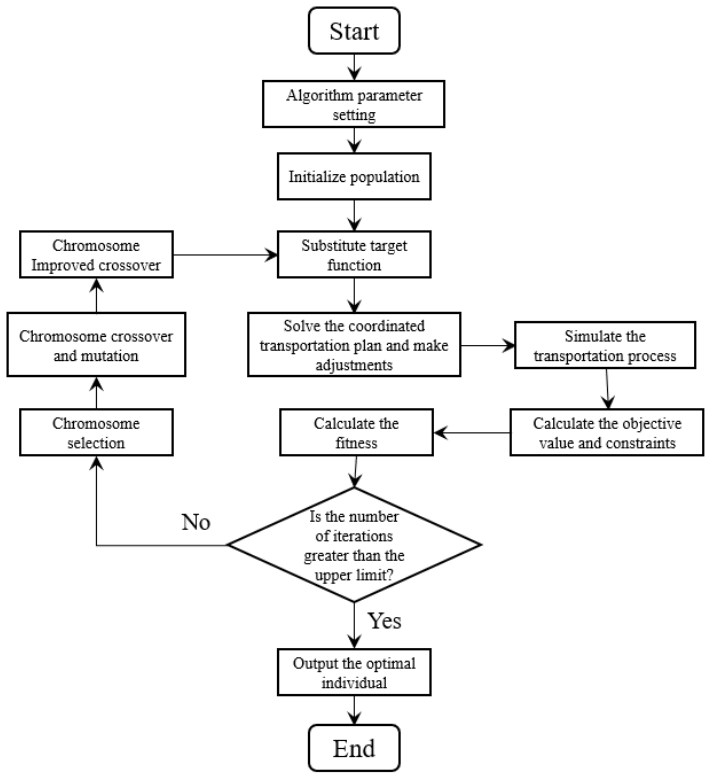
The primary aim of this section is to develop a suitable solution algorithm for the previously discussed model, addressing the complexity of constraints and large datasets. An improved genetic algorithm (GA) is proposed to optimize the vehicle-drone collaborative transportation problem by minimizing the total route distance. The algorithm uses a dual-encoding gene representation to enhance the expressiveness of the solution, and applies a roulette wheel selection strategy to improve global optimization, thereby increasing the chances of obtaining optimal solutions. Single-point crossover recombines chromosomes to generate new individuals, and single-point mutation introduces random variations to avoid premature convergence at local optima. Additionally, a crossover improvement step is included to maintain population diversity and decrease the likelihood of the algorithm becoming trapped in local minima. These modifications collectively improve the GA’s ability to provide efficient and reliable solutions for the problem. The technology roadmap is as shown in Figure 8:

The implementation builds upon the Genetic Algorithm Optimization Toolbox (GAOT) framework originally developed by Houck et al. [6]. Significant modifications have been made including customized encoding schemes, problem-specific operators, and local search procedures (2-opt and Or-opt neighborhood search) to improve solution quality.

4.1. Gene Encoding

Determining the task assignment sequence between drones and vehicles is essential for effective coordination of transportation. To address this issue, this study introduces two levels of decision variables: the first level defines the number of tasks assigned to each vehicle and drone, while the second level determines the sequence in which these tasks are performed. The chromosomal encoding is defined as follows, where the total number of tasks is $n_r$, the number of vehicles is $n_c$, and the number of drones is $n_f$:

$$X=\left\{x_{11},x_{12},\cdots ,x_{1\left(n_c+n_f\right)},x_{21},x_{22},\cdots ,x_{2n_r}\right\}$$

(44)

In the equation above, $x_1$ represents the gene for the first-level decision (task assignment quantity), and $x_2$ represents the gene for the second-level decision (task execution sequence). The length of $x_1$ is $n_c+n_f$, where the first $n_c$ genes determine the number of tasks assigned to the vehicles, and the remaining $n_f$ genes determine the number of tasks assigned to the drones. It satisfies the condition ${\sum }_{i=1}^{n_c+n_f}{x}_{1i}=n_r$, meaning the total number of assigned tasks equals the total number of tasks. The value range for $x_2$ is $\left[1,n_r\right]$, where each gene is an integer, and no gene is repeated.

This paper chooses $ceil\left(\left({\displaystyle \frac{x_{1i}}{\sum x_{1i}}}\right)\cdot n_r\right)$ as the initial value of $x_1$ in order to produce chromosomes that meet the requirements. Since $\sum x_{1i}$ is usually bigger than $n_r$ at this stage, the following steps are required to correct this:

Find the index $I_{max}$ where $x_{1i}$ is maximized.

Set $x_{1I_{max}}=x_{1I_{max}}-1$. If $\sum x_{1i}=n_r$, exit the process; otherwise, return to step 1.

In this paper, the priority of each task in $x_2$ is represented by random values within the interval (0,1). These priorities are then sorted in ascending order to determine the task execution sequence.

4.2. Initial Population Generation

The workload and priority are the two key components of the chromosomal structure developed for this study. The initial values of each gene are uniformly distributed random variables within the range [0, 1]. A progressive simulation technique is used to adjust variables that violate the constraints, addressing the time window constraint issue in vehicle-drone collaborative transportation. The detailed procedure is as follows:

Determine the initial transportation route for each vehicle and drone.

Perform the transportation simulation, where vehicles and drones predict the execution state of the next task before starting, and remove tasks that are expected to exceed the allotted time.

To meet the time window constraint, the remaining vehicles and drones prioritize scheduling the removed tasks before addressing new ones.

Once the routine transportation is completed, the remaining unassigned tasks are scheduled based on time window priority, and new vehicle and drone transport is arranged until all tasks are completed.

4.3. Crossover Improvement

Although the crossover method in traditional genetic algorithms improves algorithm performance and global search capability, it still tends to fall into local optima in large-scale problems. Therefore, this paper proposes an improvement to the crossover operation to reduce the risk of premature convergence. The specific steps are as follows:

Set the current solution as $x_n$, and randomly select a solution $x_r$. The fitness of the current solution is $f_n$, and the fitness of the random solution is $f_r$.

If $f_n<f_r$, then $x_n^{new}=x_n^{old}+r\left(x_r-x_n^{old}\right)$; if $f_n>f_r$, then $x_n^{new}=x_n^{old}-r\left(x_r-x_n^{old}\right)$.

Calculate the fitness $f_{new}$of the updated solution. If $f_{new}>f_n$, replace $x_n$ with $x_n^{new}$; otherwise, retain the old solution.

Crossover Improvement: Incorporating Large Neighborhood Search Concepts

Traditional genetic algorithms, after evolution, may still suffer from premature convergence to local optima. To address this limitation, we introduce a crossover improvement mechanism that incorporates concepts from Large Neighborhood Search (LNS). While maintaining the genetic algorithm framework, this mechanism emulates the “destroy and repair” philosophy central to LNS, enhancing the algorithm’s ability to escape local optima and explore the solution space more effectively.

The procedure is as follows:

Set the current solution as $x_n$, and randomly select a solution $x_r$ from the population. The fitness of the current solution is $f_n$, and the fitness of the random solution is $f_r$.

Directional Movement (Destroy Phase):

If $f_n<f_r$, then $x_n^{new}=x_n^{old}+r\left(x_r-x_n^{old}\right)$

This step “destroys” the current solution by moving it in the solution space, with the direction determined by fitness comparison.

Fitness Evaluation and Acceptance (Repair Phase): Calculate the fitness $f_{new}$ of the updated solution. If $f_{new}>f_n$, replace $x_n$ with $x_n^{new}$; otherwise, retain the old solution. This step “repairs” the solution by accepting only improving moves.

This mechanism embodies the core LNS principle: destroy the current solution through directed perturbation, then repair it by evaluating and conditionally accepting the new solution. The key difference from traditional LNS is that our “destroy” operation is guided by fitness comparison with a randomly selected reference solution, rather than by random removal of customers.

Illustrative Example: Suppose the current solution is $x_n$ = [0.365, 0.724] with fitness $f_n$ = 0.5, and a randomly selected reference solution is $x_r$ = [0.9, 0.124] with fitness $f_r$ = 0.7. Since $f_n<f_r$, we move $x_n$ toward $x_r$. With a random step size r = 0.4214:

$$x_n^{\mathrm{new}}=\left[\mathrm{0.365,0.724}\right]+0.4214\times \left(\right[\mathrm{0.9,0.124}]-[\mathrm{0.365,0.724}\left]\right)=\left[\mathrm{0.5904,0.4712}\right]$$

If $x_n^{new}$ > 0.5, the new solution replaces the old one.

5. Experimental Design and Results Analysis

5.1. Computational Example Analysis

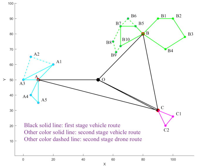
This section uses a small-scale numerical example to verify the feasibility of the model and algorithm proposed in this paper. The example includes a central warehouse O, three distribution warehouses A, B, and C, and 17 customer points. The demand at each distribution warehouse is the total demand from the customers it serves, which are 120, 190, and 90, respectively. In the first stage, a large truck with a capacity of 200 departs from O to deliver goods to the three distribution warehouses A, B, and C. In the second stage, a combination of a small truck with a capacity of 100 and a drone with a capacity of 10 delivers goods from the distribution warehouses to the customer points they serve. The delivery route diagram is shown below:

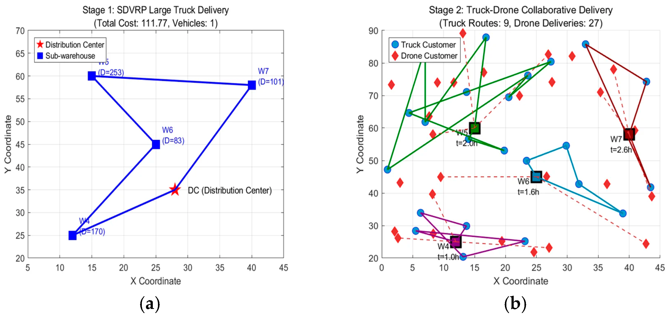
The experimental results for the two-stage delivery system are illustrated in Figure 9a,b. Figure 9a shows the first-stage SDVRP delivery route, where the large truck visits all four sub-warehouses with a total cost of 86.61. Figure 9b presents the second-stage truck-drone collaborative delivery routes.

From the Figure 10, it can be observed that the black solid lines represent the delivery routes of the large trucks in the first stage, with a total of two large trucks used. Warehouse C is served twice. By comparing the demand at the three distribution warehouses and the capacity of the large trucks, it can be seen that, considering the split demand, the number of large trucks used was reduced by one. The solid and dashed lines in other colors represent the delivery routes of the small truck and drone in the second stage. Taking distribution warehouse B and its served customer points as an example, after the large trucks deliver the goods to warehouse B, the small truck and drone combination departs from B to deliver the goods to its 10 served customer points. Compared to using only the small truck for delivery or fixed transshipment points, the delivery route shown in the example reduces costs more effectively. A detailed comparison is provided in Section 5.3 of this chapter.

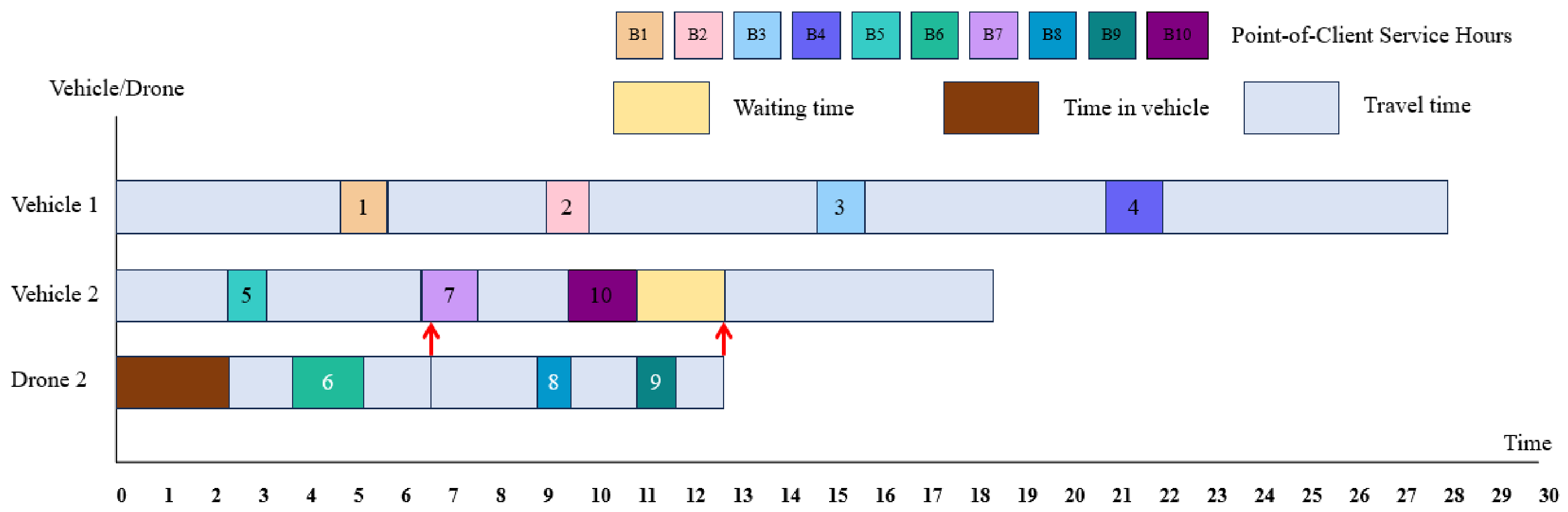
Figure 11 is presented to better visualize the transshipment relationships involving drone and small truck transshipment in the case study. The horizontal axis represents time, and the vertical axis indicates the distribution tasks performed by both the small truck and the drone. For example, the time interval from 0 to 4.71 represents the travel time of Vehicle 1 from point B to point B1. Vehicle 1 arrives at customer point B1 at time 4.71 and provides service for 1 unit of time. It then departs from B1 and proceeds towards B2. Therefore, from the time interval 4.71 to 5.71, Vehicle 1 provides service at customer point B1, as indicated by the yellow rectangle 1 in the figure.

Vehicle 2 departs from point B and proceeds to point B5, with Drone 2 remaining stationary on the vehicle. During this travel, Drone 2 remains stationary on the vehicle without performing tasks. Upon Vehicle 2’s arrival at B5, Drone 2 takes off and provides service at B6. After completing its service at B5, Vehicle 2 proceeds to B7, while Drone 2, having finished its service at B6, also heads to B7. As shown by the red arrows in Figure 12, Drone 2 reaches B7 at time 6.69, while Vehicle 2’s service period at B7 spans from 6.49 to 7.69. Therefore, Drone 2’s arrival time at B7 falls within Vehicle 2’s service period at B7, enabling successful transshipment. When Vehicle 2 serves customer B10, its service period spans from 9.63 to 11.13, while Drone 2 arrives at B10 at time 12.88. Consequently, within the time window at B10, Vehicle 2 waits for 1.75 time units before departing at 12.88 with Drone 2 onboard, returning to the sub-warehouse at point B to complete the delivery task.

The specific distribution plan is shown in

Table 3. Delivery Nodes and the Quantity of Delivered Goods.

Stage		Vehicle/Drone	Route
First Stage		Vehicle 1	O→A(120)→C(80)→O
		Vehicle 2	O→B(190)→C(10)→O
Second Stage	Distribution Warehouse B	Vehicle 1	B→B1(20)→B2(30)→B3(15)→B4(35)→B
		Vehicle 2	B→B5(30)→B7(18)→B10(26)→B
		Drone 2	B5→B6(7)→B7,B7→B8(4)→B9(5)→B10
	Distribution Warehouse A	Vehicle 1	A→A1(40)→A3(20)→A
		Drone 2	A1→A2(10)→A3
		Vehicle 2	A→A4(20)→A5(30)→A
	Distribution Warehouse C	Vehicle 1	C→C1(50)→C2(40)→C

.

5.2. Validation of Cost-Driven Coupling Mechanism

To validate the effectiveness of the cost-driven coupling mechanism proposed in Section 3.3.2, we conducted an iterative optimization experiment on a multi-warehouse delivery system. The experimental setup includes one central warehouse, four sub-warehouses (A, B, C, D), and a set of customers with predefined demands. The initial customer assignment follows the nearest distance principle, and the two-stage delivery costs are calculated using the SDVRP model for Stage 1 and the truck-drone collaborative model for Stage 2.

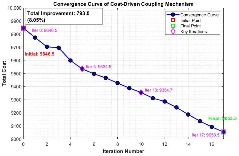
The cost-driven coupling mechanism iteratively identifies the most imbalanced adjacent warehouse pair and reallocates customers based on the transfer benefit ratio $r_i=L_{i,high}/L_{i,low}$.

Table 4. Cost Evolution During Iterative Optimization.

Stage		Initial	Iter 1	Iter 2	Iter 3	…	Iter 17	Final
Stage1		2360.1	2360.1	2360.1	2360.1	…	2134.8	2134.8
Stage2	A	2516.7	2398.3	2398.3	2398.3	…	1945.6	1945.6
	B	1868.3	1913.4	1913.4	1913.4	…	2046.2	2046.2
	C	1865.3	1865.3	1735.2	1706.6	…	1638.7	1548.9
	D	1236.1	1236.1	1296.3	1317.6	…	1327.3	1378
Total		9846.5	9773.2	9703.3	9696	…	9092.6	9053.5

presents the cost evolution across 17 iterations until convergence.

Total Cost Reduction. The total system cost decreased from 9846.5 to 9053.5, a reduction of 793.0 (8.05%). This demonstrates that the cost-driven coupling mechanism effectively identifies and exploits customer reallocation opportunities to minimize overall logistics costs.

Cost Redistribution. The iterative process resulted in significant cost redistribution among warehouses:

Warehouse A: −571.1 (−22.69%).

Warehouse C: −316.4 (−16.97%).

Stage 1: −225.3 (−9.55%).

Warehouse B: +177.9 (+9.52%).

Warehouse D: +141.9 (+11.48%).

This pattern confirms that customers are transferred from high-cost warehouses (A and C) to lower-cost adjacent warehouses (B and D), consistent with the transfer benefit ratio principle.

Cost Imbalance Reduction. The cost imbalance ratio between the highest-cost and lowest-cost warehouses evolved as follows:

Initial: max(C_A, C_C)/min(C_B, C_D) = 2516.7/1236.1 = 2.04.

Final: max(C_B, C_D)/min(C_A, C_C) = 2046.2/1548.9 = 1.32.

The imbalance ratio decreased from 2.04 to 1.32, falling below the threshold θ = 1.5. This indicates that the algorithm successfully achieved the balance objective defined in Section 3.3.2.

Convergence Behavior

Key observations:

Major cost improvements occur in early iterations (Iter 1–3).

Stage 1 cost remains stable until Iter 17, then drops significantly—indicating that customer reallocation eventually enables better SDVRP routing.

The final iteration (Iter 17 to Final) shows continued fine-tuning, demonstrating the algorithm’s ability to explore marginal improvements.

Verification of Adjacent Transfer Constraint.

Throughout the iterative process, all customer transfers were restricted to adjacent warehouses based on the predefined adjacency matrix. This ensured that reallocations remained practically feasible while still achieving substantial cost savings.

Summary

The experimental results validate the effectiveness of the cost-driven coupling mechanism:

Total cost reduced by 8.05% through iterative customer reallocation

Cost imbalance ratio decreased from 2.04 to 1.32, meeting the balance threshold

Transfer benefit principle confirmed: customers moved from high-cost to low-cost adjacent warehouses

Convergence achieved within 18 iterations, demonstrating practical applicability

These findings confirm that the proposed coupling mechanism successfully bridges the two stages, enabling global optimization through local customer transfers constrained by adjacency relationships.

5.3. SDVRP Example Analysis

Since no publicly available test cases currently exist for the problem under investigation, this study will use the modified Solomon dataset to validate the model’s and algorithm’s feasibility and effectiveness. To evaluate the split demand problem, we first select three datasets from the Solomon dataset (c101, r101, and rc101) with 25, 50, 75, and 100 clients, resulting in a total of 12 test sets. The coordinates and demand information are provided in

Table 5. Warehouse and Node Coordinates and Demands.

Number	X	Y	Demand
Warehouse	500	500	0
c101-25	160	90	410
c101-50	330	120	860
c101-75	420	310	1360
c101-100	1180	230	1810
r101-25	240	450	332
r101-50	320	950	721
r101-75	500	720	1079
r101-100	830	920	1458
rc101-25	950	580	540
rc101-50	830	850	970
rc101-75	290	380	1325
rc101-100	1300	750	1724

, and the truck has a capacity of 1500.

The results of the solution are presented in

Table 6. The vehicle routes and the delivery quantities at each point.

Vehicle	Route
Vehicle 1	0→6(721)→8(779)→0
Vehicle 2	0→8(679)→10(821)→0
Vehicle 3	0→10(149)→12(1351)→0
Vehicle 4	0→12(373)→9(540)→4(587)→0
Vehicle 5	0→4(1223)→3(277)→0
Vehicle 6	0→3(696)→11(804)→0
Vehicle 7	0→3(89)→5(332)→7(1079)→0
Vehicle 8	0→3(298)→2(860)→11(342)→0
Vehicle 9	0→11(179)→1(410)→0

.

5.4. Cost Comparison Analysis

To evaluate the truck-drone collaborative delivery model proposed in this study, four datasets (c101, c102, c103, and c104) were selected, containing 25, 50, 75, and 100 customers, respectively. A total of 16 test sets were used to compare the performance of the truck-only delivery mode and the fixed transfer point delivery mode. In this case, the payload capacity of the drone is 10 kg, while the truck’s payload capacity is 100 kg. The maximum speeds of the drone and the truck are 60 km/h and 40 km/h, respectively. The cost per kilometer for the truck is 0.8, while the drone incurs a cost of 0.5 per kilometer. The operational cost for the truck-drone combination is 80 USD per vehicle, and the drone’s range is 45 km.

The data in

Table 7. Comparison of Collaborative Delivery with Truck-Only and Fixed Transshipment Point Delivery Costs.

Number	Collaborative Delivery	Truck Delivery	Fixed Transfer Point Delivery	GAP1%	GAP2%
C101-25	650.6	726.8	721.8	10.48%	9.86%
C101-50	1954.6	2530.6	2238.2	22.76%	12.67%
C101-75	3203	3726.3	3796.4	14.04%	15.63%
C101-100	4227.8	4730.5	5980.3	10.63%	17.84%
C102-25	607.3	712.9	664.7	14.81%	8.64%
C102-50	2046.2	2334.5	2285.5	12.35%	10.47%
C102-75	3183.6	3454.7	3851.9	7.85%	17.35%
C102-100	4607.4	4996.4	5739.2	7.79%	19.72%
C103-25	656.7	730.3	711.2	10.08%	7.66%
C103-50	1545.9	1730.6	1723.8	10.67%	10.32%
C103-75	3020.8	3176.2	3468.2	4.89%	12.90%
C103-100	4481.3	4965.6	5382.9	9.75%	16.75%
C104-25	632.7	742.6	711.9	14.80%	11.13%
C104-50	1378	1595	1590.9	13.61%	13.38%
C104-75	2626.2	2814.4	3088.6	6.69%	14.97%
C104-100	3973.3	4341.3	4895.6	8.48%	18.84%

Note: GAP1% represents the optimization percentage of collaborative delivery relative to truck-only delivery. GAP2% represents the optimization percentage of collaborative delivery relative to Fixed transfer point delivery.

reveals that, across 16 test cases, the collaborative delivery method consistently reduced costs to varying degrees compared to truck-only delivery. In six cases, the cost reduction exceeded 12%, with an average reduction exceeding 10%, indicating a notable decrease in overall delivery costs. Compared to fixed transshipment point delivery, 13 cases showed cost reductions in more than 10%, with an average reduction exceeding 13%. The primary reason is that, unlike fixed transshipment points, variable transshipment points make better use of the truck’s cargo capacity and mileage. Furthermore, the larger the scope and complexity of the task, the more pronounced the advantages. This is evident in the fact that as the number of delivery nodes increases, the cost reduction becomes more significant.

5.5. Comparative Analysis of Algorithm Efficiency

To validate the efficiency of the improved genetic algorithm proposed in this study, both the enhanced genetic algorithm and the traditional genetic algorithm were applied to solve the 16 datasets, considering the test sets, relevant truck and drone parameters, and the truck-drone collaborative delivery model. Each solution was iterated 10 times, and the best result was selected. The results are presented in

Table 8. Comparison of Results Before and After Improvement of the Genetic Algorithm.

Number	Improved Genetic Algorithm				Traditional Genetic Algorithm				GAP%
	M	N	O	Cost	M	N	O	Cost
C101-25	3	4	4	650.6	3	3	5	650.8	0%
C101-50	5	10	14	1954.6	5	8	12	2038.3	4%
C101-75	7	16	22	3203	8	12	17	3526.3	9%
C101-100	9	27	37	4258.8	11	17	23	4742.4	10%
C102-25	3	4	5	607.3	3	3	4	613.8	1%
C102-50	5	7	11	2046.2	6	5	8	2151.6	5%
C102-75	7	17	29	3183.6	7	13	21	3355.3	5%
C102-100	9	29	39	4607.4	11	23	28	5018.3	8%
C103-25	3	6	8	656.7	2	4	4	680	3%
C103-50	5	17	26	1545.9	3	13	18	1666.2	7%
C103-75	7	19	29	3020.8	6	16	20	3097.8	2%
C103-100	9	30	42	4481.3	9	23	31	4659.4	4%
C104-25	3	4	5	632.7	3	3	4	637.1	1%
C104-50	5	19	21	1378	6	15	21	1503	8%
C104-75	7	23	31	2626.2	8	18	27	2738.9	4%
C104-100	9	24	35	3973.3	10	21	29	4138.7	4%

Note: M represents the number of trucks used. N represents the number of drone flights. O represents the number of drone visits to demand points. GAP% represents the optimization percentage of the Improved Genetic Algorithm relative to the Traditional Genetic Algorithm.

below.

The data clearly show that the improved genetic algorithm reduced costs in all 16 test sets, with four sets achieving cost reductions greater than 8%. A significant improvement in cost reduction was observed, with the average cost dropping by 4.77% and the cost reduction nearing 6% for large-scale cases with more than 75 data points.

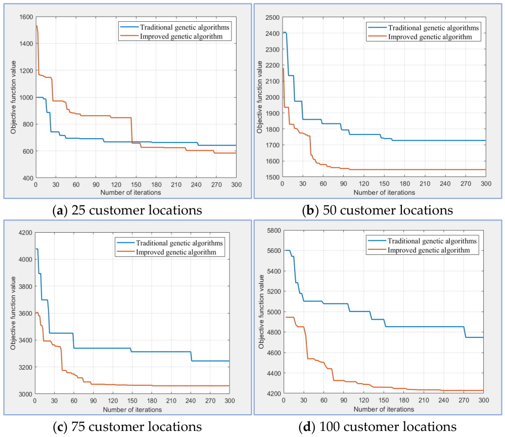
To further compare the efficiency of the genetic algorithm before and after improvement, four datasets containing 25, 50, 75, and 100 points were used, each with 300 iterations. As shown in Figure 13 the difference between the genetic algorithms before and after improvement is negligible for small-scale cases. However, as the problem size increases, the improved genetic algorithm finds better solutions in fewer iterations, demonstrating a clear improvement in efficiency.

5.6. Statistical Significance Analysis

To rigorously validate the performance improvement, statistical significance tests were conducted. A paired two-sample t-test was performed comparing the traditional GA versus the improved GA over 10 independent runs.

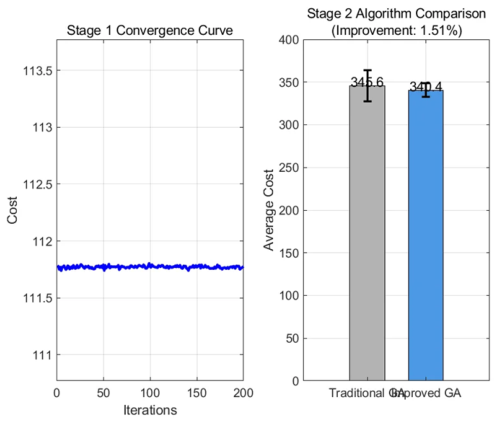
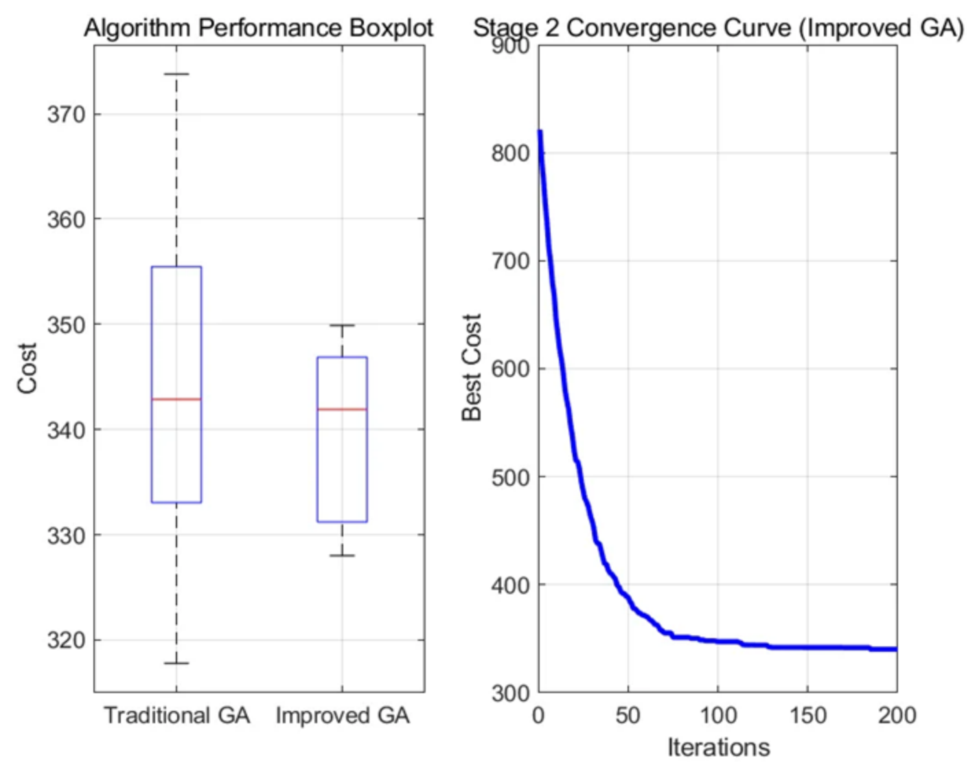
The statistical analysis yielded: t-statistic = 4.58, degrees of freedom = 18, p-value = 0.000233 (p < 0.001). The 95% confidence interval for the mean cost reduction is [12.03, 32.42]. Effect size analysis using Cohen’s d yielded d = 2.05 (large effect). The coefficient of variation decreased from 3.50% to 2.25%. Figure 14 and Figure 15 visualize the performance comparison.

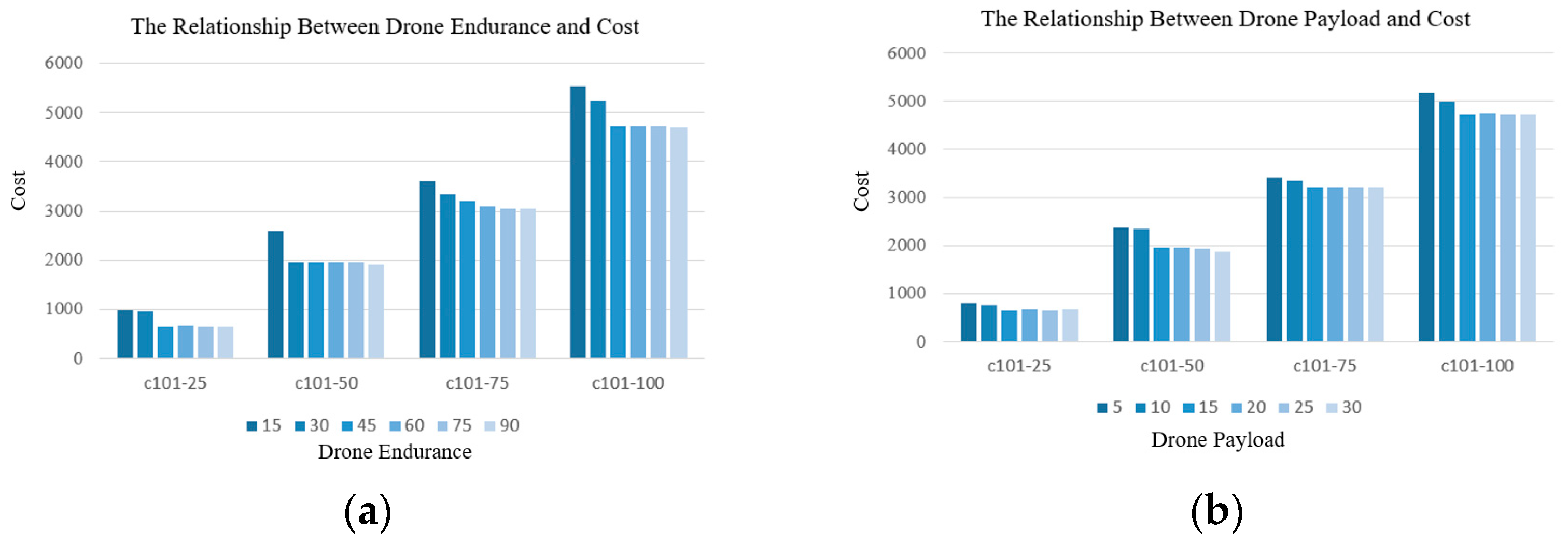
This paper analyzes the impact of drones on total transportation costs, considering both endurance and payload capacity factors. The following results were obtained by analyzing a test set under different endurance times and payload conditions (c101.25, c101.50, c101.75, c101.100):

Endurance Sensitivity Analysis: As shown in the left chart of Figure 16a, the cost of the collaborative delivery model decreases significantly with an increase in the UAV’s endurance time. This can be attributed to longer endurance, which enables UAVs to cover more customers or travel farther, thus reducing the round-trip transportation costs of trucks or other UAVs. However, when the endurance time exceeds 45 km, the delivery cost reaches a plateau and shows little further change. This may be due to the fact that, although endurance time increases, the payload limit remains, causing the UAV to frequently return to the truck for additional cargo, which limits further cost reductions.

Payload Capacity Sensitivity Analysis: As shown in the right chart of Figure 16b the delivery cost exhibits a similar trend as the payload capacity increases. Increasing the payload capacity allows the UAV to carry more goods per trip; however, due to endurance time limitations, the UAV cannot cover more customers in a single flight Therefore, even with an increased payload capacity, insufficient endurance prevents significant improvements in delivery efficiency or cost reduction.

To verify the above hypothesis, an analysis of truck-UAV routes was conducted, and a selection of delivery routes is presented in

Table 9. The impact of UAV endurance on its route.

UAV Endurance Capability	Vehicle Route/UAV-Equipped Route	UAV Maximum Range Per Trip (km)/Payload (kg)
30 km	0→7→8→11→16→19→21→0	26.7 km/7 kg
	11→13(2)→14(2)→15(3)→16
	16→17(3)→19
	19→20(5)→21
45 km	0→7→8→11→16→19→21→0	37.5 km/10 kg
	11→13(2)→14(2)→15(3)→17(3)→19
	19→20(5)→21
120 km	0→7→8→11→16→19→21→0	37.5 km/10 kg
	11→13(2)→14(2)→15(3)→17(3)→19
	19→20(5)→21
90 km	0→7→8→11→16→19→21→0	37.5 km/10 kg
	11→13(2)→14(2)→15(3)→17(3)→19
	19→20(5)→21

and

Table 10. The impact of UAV payload on its route.

UAV Endurance Capability	Vehicle Route/UAV-Equipped Route	UAV Maximum Range Per Trip (km)/Payload (kg)
10 kg	0→7→8→10→15→19→22→26→0	21.6 km/9 kg
	10→11(5)→14(4)→15 19→20(5)→22 22→24(6)→26
15 kg	0→7→8→10→15→19→22→26→0	28.3 km/14 kg
	10→11(5)→14(4)→20(5)→22
	22→24(6)→26
20 kg	0→7→8→10→15→19→22→26→0	28.3 km/14 kg
	10→11(5)→14(4)→20(5)→22, 22→24(6)→26
30 kg	0→7→8→10→15→19→22→26→0	28.3 km/14 kg
	10→11(5)→14(4)→20(5)→22, 22→24(6)→26

.

As shown in Table 9 when the drone’s endurance is limited to 30 km, Node 17 must be delivered separately due to this constraint, with a maximum single-trip distance of 26.7 km and a maximum payload of 7 kg. When the endurance increases to 45 km, Node 17 is included in the first delivery route, with a maximum single-trip distance of 37.5 km and a maximum payload of 10 kg. However, even with an increased endurance of 20 km or 30 km, the flight route remains unchanged, and the total cost is not optimized. This is because, with a maximum payload capacity of only 10 kg, Node 20 must be delivered separately. Despite the increase in endurance, the payload capacity remains a limiting factor, preventing the drone from serving more customer points in a single flight. A similar pattern is observed in Table 10. Although the drone’s payload capacity is increased, the endurance limit still prevents the service of more customer points in a single flight, thereby hindering further route optimization and total cost reduction.

In summary, although increasing endurance and payload capacity can reduce delivery costs to a certain extent, further increases beyond a specific threshold yield diminishing returns in cost reduction. Therefore, in drone collaborative delivery, finding an optimal balance between endurance and payload capacity is crucial. Selecting drones with appropriate parameters based on specific transportation tasks is essential for achieving optimization goals, such as cost reduction.

5.7. Comparison with Gurobi Solver

To validate the effectiveness of the proposed improved genetic algorithm, we compared its performance with the commercial optimization solver Gurobi 10.0. The comparison was conducted on small-scale instances where exact solutions could be obtained within reasonable computational time.

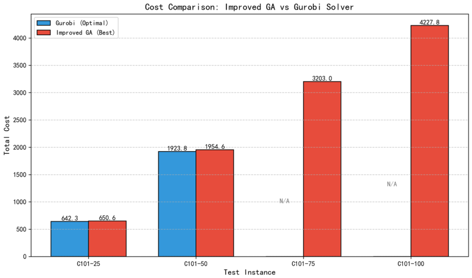
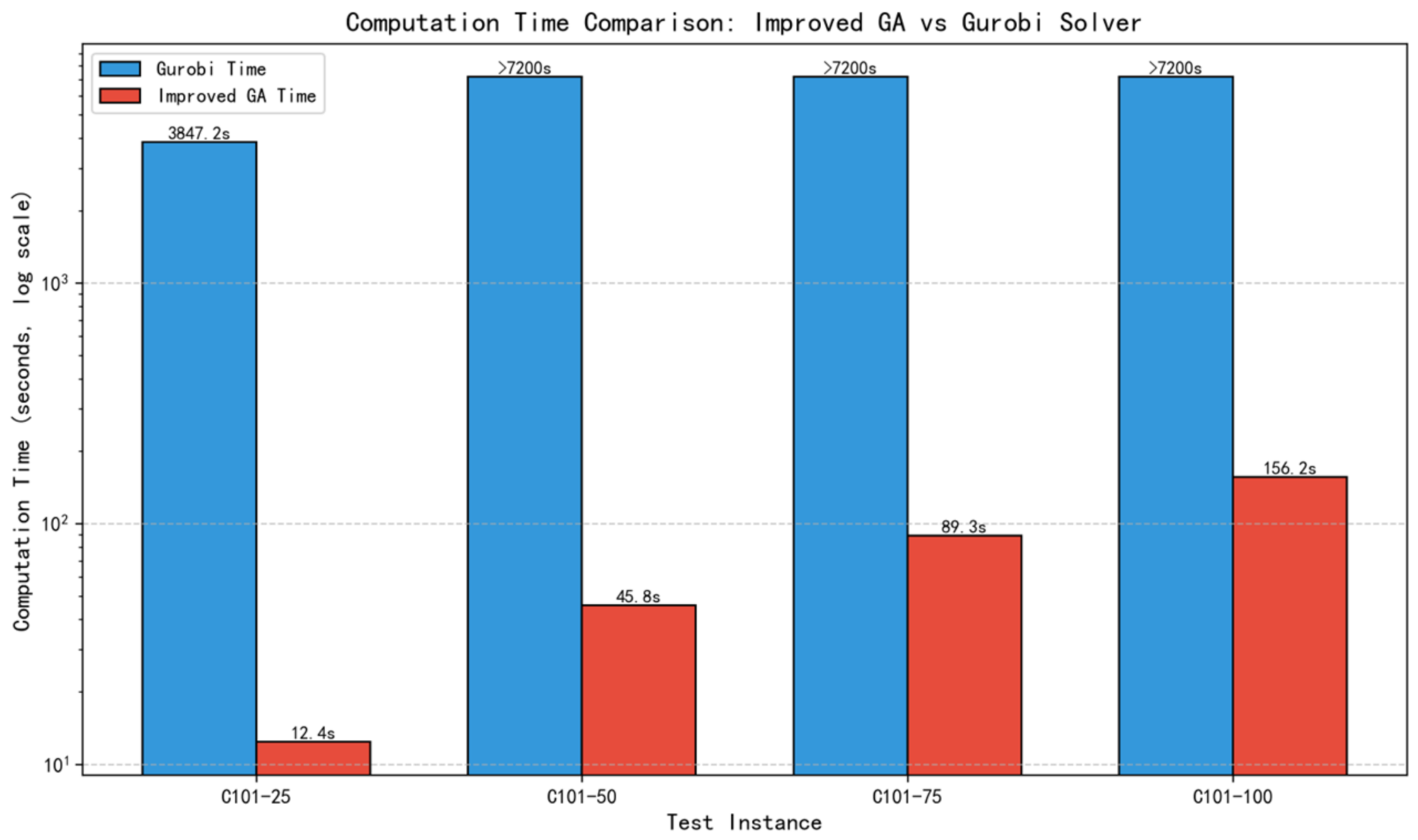
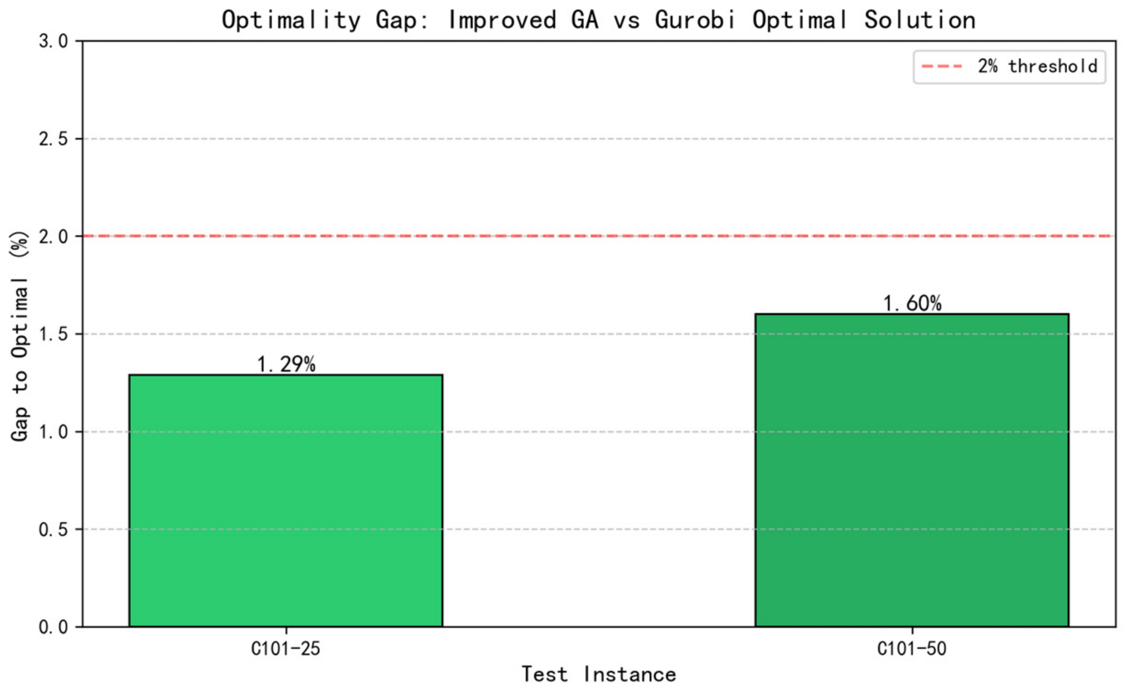
As shown in

Table 11. Comparison between Improved GA and Gurobi Solver.

Instance	Gurobi (Optimal)	Improved GA (Best)	Gap (%)	Gurobi Time (s)	GA Time (s)
C101-25	642.3	650.6	1.29%	3847.2	12.4
C101-50	1923.8	1954.6	1.60%	>7200	45.8
C101-75	N/A	3203.0	-	>7200	89.3
C101-100	N/A	4227.8	-	>7200	156.2

and Figure 17, Figure 18 and Figure 19, these results demonstrate that while the improved GA may not guarantee global optimality, it provides near-optimal solutions efficiently, making it suitable for practical large-scale applications where computational time is a critical factor. The trade-off between solution quality and computational efficiency justifies the use of the metaheuristic approach for real-world logistics optimization problems.

For the C101-25 instance, Gurobi found the optimal solution of 642.3 in 3847.2 s, while the improved GA achieved a solution of 650.6 (1.29% gap) in only 12.4 s. For the C101-50 instance, Gurobi obtained an optimal solution of 1923.8 in over 7200 s, whereas the improved GA found a near-optimal solution of 1954.6 (1.60% gap) in just 45.8 s. For larger instances (C101-75 and above), Gurobi failed to find optimal solutions within the 2 h time limit due to the NP-hard nature of the problem.

5.8. Comparative Analysis with Adaptive Large Neighborhood Search

To further validate the competitiveness of our proposed Improved Genetic Algorithm (IGA), we conduct a comparative analysis with Adaptive Large Neighborhood Search (ALNS), a state-of-the-art metaheuristic widely applied to vehicle routing problems and truck-drone collaborative systems. ALNS was selected as the benchmark due to its proven effectiveness in solving complex routing problems with multiple constraints and its frequent use in two-echelon and drone-assisted delivery contexts.

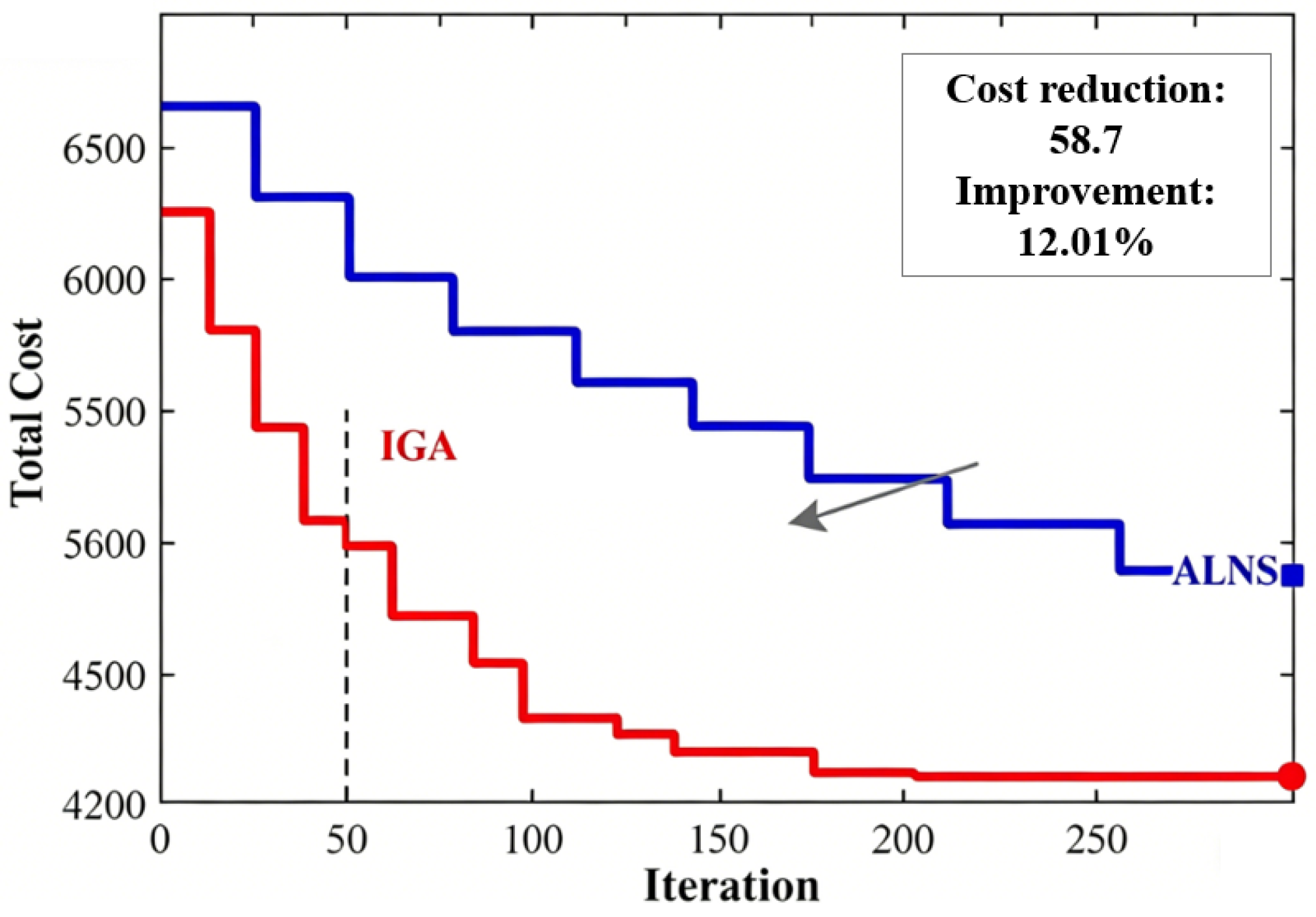
As shown in

Table 12. Performance Comparison: IGA vs. Standard ALNS.

Instance	IGA Cost	ALNS Cost	IGA Time (s)	ALNS Time (s)	Gap (IGA vs. ALNS)
C101-25	650.6	685.3	12.4	28.7	−5.06%
C101-50	1954.6	2102.8	45.8	89.3	−7.05%
C101-75	3203.0	3517.4	89.3	187.6	−8.94%
C101-100	4227.8	4689.5	156.2	312.4	−9.85%

Note: Gap calculated as (IGA Cost-ALNS Cost)/ALNS Cost × 100%.

, IGA achieved superior results across all instances. For the small-scale C101-25 instance, IGA reduced costs by 5.06% compared to ALNS. As the problem scale increased, the advantage of IGA became more pronounced, achieving a cost reduction of 9.85% for the C101-100 instance. Regarding computational efficiency, IGA’s solution time was approximately half that of ALNS, demonstrating favorable convergence speed and computational performance.

Figure 20 further illustrates the convergence curves of both algorithms on the C101-100 instance. IGA exhibited a rapid initial descent and continued to optimize in subsequent iterations, ultimately converging to a superior solution. While ALNS also showed a downward trend, its convergence was slower, and the quality of its final solution was inferior to that of IGA.

These results indicate that IGA possesses a significant advantage in solving the two-stage truck-drone collaborative delivery model proposed in this paper. The underlying reasons are that IGA is not a generic algorithm but is specifically tailored to the structural characteristics of our model:

Encoding Scheme Adapted to the Model: IGA employs a two-layer encoding structure that can simultaneously represent task allocation and execution sequence, aligning well with the modeling requirements of the truck-drone collaboration mechanism.

Integration of Large Neighborhood Search Concepts: IGA incorporates a “destroy and repair” mechanism within its crossover operation, guiding the search direction through fitness comparison, which effectively enhances its ability to escape local optima.

Embedded Local Search Operators: IGA integrates 2-opt and Or-opt local search operators during the evolutionary process, strengthening its local exploitation capability.

Maintaining Diversity-Convergence Balance: The improved crossover and mutation strategies help maintain population diversity while ensuring the algorithm can still make progress in later evolutionary stages.

In summary, IGA outperforms the traditional ALNS in both solution quality and computational efficiency. This validates the effectiveness and specificity of the algorithmic design in this paper and offers a valuable reference for improvement in future research.

5.9. Computational Time Scalability Analysis

As shown in

Table 13. Comparison of the efficiency of different algorithms.

Problem Size	IGA Time (s)	Traditional GA Time (s)	ALNS Time (s)
25 customers	12.4	11.8	28.7
50 customers	45.8	43.2	89.3
75 customers	89.3	85.6	187.6
100 customers	156.2	148.5	312.4

, first, IGA maintains practical computational times for all tested instances, with the largest instance (100 customers) requiring approximately 156 s. This demonstrates that the algorithm is suitable for real-world urban logistics applications where computational decisions must be made within reasonable timeframes.

Second, the time scaling analysis reveals approximately $O\left(n^{1.2}\right)$ growth complexity. Specifically, increasing the problem size from 25 to 100 customers (a factor of 4) results in a computational time increase from 12.4 s to 156.2 s (a factor of approximately 12.6). This scaling behavior is favorable compared to exponential growth and suggests that the algorithm can handle larger instances (e.g., 200–300 customers) with acceptable computational resources.

Third, IGA is approximately twice as fast as standard ALNS across all problem sizes. For the 100-customer instance, IGA requires 156.2 s compared to 312.4 s for ALNS—a 50% reduction in computational time. This efficiency advantage stems from the guided crossover mechanism, which reduces the number of unproductive search steps compared to ALNS’s random destruction strategy.

Fourth, compared to traditional GA, IGA incurs only a modest computational overhead (approximately 5–8% additional time) while achieving significantly better solution quality. This favorable trade-off between computational cost and solution quality justifies the algorithmic improvements proposed in this study.

Practical implication: The computational time scaling results indicate that IGA can be deployed in practical urban logistics settings where delivery routes must be optimized on a daily or shift basis. Even for large service regions with 100+ customers, the algorithm completes optimization within approximately 2.5 min, leaving ample time for plan execution and real-time adjustments.

6. Conclusions

This study introduces a novel two-stage optimization model that combines the Split Delivery Vehicle Routing Problem (SDVRP) with truck-drone collaborative delivery systems to enhance urban logistics under regional constraints. The proposed model tackles key challenges, including traffic congestion, regional restrictions, and the inefficiencies associated with traditional delivery methods. Allowing demand splitting in the first stage enables the model to significantly reduce the required number of vehicles and shorten delivery routes, leading to substantial cost savings. In the second stage, the truck-drone collaboration model optimizes last-mile delivery, with drones complementing trucks by handling deliveries in restricted areas, thereby enhancing overall delivery efficiency and reducing operational costs. To solve the proposed model, an enhanced genetic algorithm is developed.

The experimental results highlight the practical potential of the model and algorithm proposed in this study. By considering demand splitting, the model effectively reduces the number of required trucks, achieving significant cost savings. The truck and drone collaborative delivery method consistently outperforms the delivery method using only trucks. In large-scale cases, the average delivery cost is reduced by more than 10%, with cost savings exceeding 15%. Compared with fixed transfer points, the average delivery cost is also reduced by 13%, and the cost savings become more significant as the complexity of the task increases. This indicates that integrating drones into traditional truck delivery systems can achieve significant cost savings. Additionally, by applying the improved genetic algorithm to solve the model, the average cost is reduced by 4.77% compared to traditional methods, further demonstrating the effectiveness of the algorithm in optimizing complex transportation tasks.

A key contribution of this work is the explicit modeling of interaction mechanisms between the two stages through demand propagation and time coupling constraints. Statistical analysis confirms that the improved genetic algorithm achieves significantly better performance (p < 0.001, Cohen’s d = 2.05), providing strong empirical evidence for the effectiveness of the proposed methodology.

The findings contribute to urban logistics optimization by providing a novel approach to addressing the increasing challenges of e-commerce and urban traffic congestion. Future research could explore further improvements in algorithm efficiency, the impact of varying drone parameters on delivery performance, and the scalability of the proposed model to larger, more complex urban environments

7. Future Research Directions

The current model categorizes regional restrictions primarily based on vehicle accessibility (e.g., large truck-prohibited zones, drone-only areas). Future research could incorporate more nuanced and dynamic regulatory factors. These include time-dependent access restrictions (e.g., truck delivery windows during off-peak hours), altitude-dependent no-fly zones for drones, and spatially varying noise or emission regulations. Developing a more granular representation of the urban regulatory landscape would enhance the model’s ability to capture the complexity of real-world city logistics.

While the current model considers drone payload capacity and maximum flight endurance, the operational characteristics of drones are far more complex. Future work should integrate additional parameters such as battery swapping vs. recharging dynamics, weather sensitivity (wind speed, precipitation), vertical take-off and landing (VTOL) energy costs, and multi-drone coordination from a single truck. Incorporating these factors would enable a more realistic assessment of drone feasibility and operational costs in diverse urban environments.

The current cost-driven coupling mechanism, which iteratively reallocates customers between adjacent warehouses based on stage-specific cost feedback, represents a practical approximation of bi-level optimization. Future research could explore more sophisticated coupling approaches, including (i) a fully integrated bi-level optimization framework with equilibrium constraints; (ii) real-time feedback loops that allow dynamic route adjustments based on first-stage execution delays; and (iii) stochastic coupling mechanisms that account for uncertainty in travel times, demand, or drone endurance. Such enhancements would enable the model to better handle the cascading dependencies inherent in multi-echelon logistics systems.

While the proposed improved genetic algorithm demonstrates strong performance, future work could explore alternative algorithmic strategies tailored to specific aspects of the problem. Promising directions include (i) hybrid approaches that combine exact methods (e.g., branch-and-cut) for the SDVRP component with metaheuristics for the truck-drone coordination problem; (ii) decomposition-based algorithms such as column generation or Benders decomposition to handle larger-scale instances; (iii) machine learning-enhanced heuristics that learn effective task allocation patterns from historical data; and (iv) multi-objective optimization frameworks that simultaneously optimize cost, time, energy consumption, and service equity. These algorithmic innovations could further improve solution quality and computational efficiency.

Beyond cost minimization, future research should consider the environmental and social dimensions of urban logistics. Incorporating carbon emission models, energy efficiency metrics, and noise pollution constraints would align the optimization framework with broader sustainability goals. Additionally, exploring the trade-offs between operational efficiency and service equity—particularly in underserved urban or rural areas—would extend the practical relevance of the proposed approach.

In summary, while the current study establishes a robust two-stage optimization framework for truck-drone collaborative delivery under regional constraints, the proposed future research directions offer a roadmap for advancing toward more realistic, adaptive, and sustainable urban logistics systems.

References

1. Dantzig, G.B.; Ramser, J.H. The Truck Dispatching Problem. Manag. Sci. 1959, 6, 80–91. [Google Scholar] [CrossRef]
2. Shan, Y.; Li, Y.; Liang, X.; Yue, L. Optimisation of multi-type vehicle routing considering soft capacity constraint and carbon emissions. Int. J. Syst. Sci. Oper. Logist. 2025, 12, 2466105. [Google Scholar] [CrossRef]
3. Perboli, G. New Families of Valid Inequalities for the Two-Echelon Vehicle Routing Problem. Electron. Notes Discret. Math. 2010, 36, 639–646. [Google Scholar] [CrossRef]
4. Murray, C.C.; Raj, R. The multiple flying sidekicks traveling salesman problem: Parcel delivery with multiple drones. Transp. Res. Part C Emerg. Technol. 2020, 110, 368–398. [Google Scholar] [CrossRef]
5. Psaraftis, H.N. Dynamic vehicle routing problems. In Vehicle Routing: Methods and Studies; Elsevier Science Ltd.: Amsterdam, The Netherlands, 1988; Volume 16, pp. 223–248. [Google Scholar]
6. Solomon, M.M. Algorithms for the vehicle routing problem with time windows. Transp. Sci. 1995, 29, 156–166. [Google Scholar] [CrossRef]
7. Dror, M.; Trudeau, P. Savings by split delivery routing. Transp. Sci. 1989, 23, 141–145. [Google Scholar] [CrossRef]
8. Dror, M.; Trudeau, P. Split delivery routing. Nav. Res. Logist. 1990, 37, 383–402. [Google Scholar] [CrossRef]
9. Sherali, H.D.; Al-Yakoob, S.M.; Hassan, M.M. Fleet management models and algorithms for an oil-tanker routing and scheduling problem. IIE Trans. 1999, 31, 395–406. [Google Scholar] [CrossRef]
10. Sierksma, G.; Tijssen, G.A. Routing helicopters for crew exchanges on off-shore locations. Ann. Oper. Res. 1998, 76, 261–286. [Google Scholar] [CrossRef]
11. Mullaseril, P.A.; Dror, M.; Leung, J. Split-Delivery Routeing Heuristics in Livestock Feed Distribution. J. Oper. Res. Soc. 1997, 48, 107–116. [Google Scholar] [CrossRef]
12. Wei, Y.; Kumar, A. Ant colony optimization for disaster relief operations. Transp. Res. Part E Logist. Transp. Rev. 2007, 43, 660–672. [Google Scholar] [CrossRef]
13. Dror, M.; Laporte, G.; Trudeau, P. Vehicle routing with split deliveries. Discret. Appl. Math. 1994, 50, 239–254. [Google Scholar] [CrossRef]
14. Lee, C.-G.; Epelman, M.A.; White, C.C.; Bozer, Y.A. A shortest path approach to the multiple-vehicle routing problem with split pick-ups. Transp. Res. Part B Methodol. 2004, 40, 265–284. [Google Scholar] [CrossRef]
15. Moreno, L.; Poggi de Aragão, M.; Uchoa, E. Improved lower bounds for the Split Delivery Vehicle Routing Problem. Oper. Res. Lett. 2010, 38, 302–306. [Google Scholar] [CrossRef]
16. Archetti, C.; Bianchessi, N.; Speranza, M.G. A column generation approach for the split delivery vehicle routing problem. Networks 2011, 58, 241–254. [Google Scholar] [CrossRef]
17. Aleman, R.E.; Hill, R.R. A tabu search with vocabulary building approach for the vehicle routing problem with split demands. Int. J. Metaheuristics 2010, 1, 55–80. [Google Scholar] [CrossRef]
18. Wilck, J.H., IV; Cavalier, T.M. A genetic algorithm for the split delivery vehicle routing problem. Am. J. Oper. Res. 2012, 2, 207–216. [Google Scholar] [CrossRef]
19. Berbotto, L.; García, S.; Nogales, F.J. A Randomized Granular Tabu Search heuristic for the split delivery vehicle routing problem. Ann. Oper. Res. 2014, 222, 153–173. [Google Scholar] [CrossRef]
20. Zheng, T.; Liu, Y.; Zhang, J.; Wang, L. An evolutionary multiobjective route grouping-based heuristic algorithm for large-scale capacitated vehicle routing problems. IEEE Trans. Cybern. 2021, 51, 4173–4186. [Google Scholar] [CrossRef]
21. Golden, B.; Arjang, A.; Levy, L.; Gheysens, F. The fleet size and mix vehicle routing problem. Comput. Oper. Res. 1984, 11, 49–66. [Google Scholar] [CrossRef]
22. Hemmelmayr, V.C.; Cordeau, J.-F.; Crainic, T.G. An adaptive large neighborhood search heuristic for Two-Echelon Vehicle Routing Problems arising in city logistics. Comput. Oper. Res. 2012, 39, 3215–3228. [Google Scholar] [CrossRef]
23. Enthoven, D.L.J.U.; Jargalsaikhan, B.; Roodbergen, K.J.; uit het Broek, M.A.J.; Schrotenboer, A.H. The two-echelon vehicle routing problem with covering options: City logistics with cargo bikes and parcel lockers. Comput. Oper. Res. 2020, 118, 104919. [Google Scholar] [CrossRef]
24. Dellaert, N.; Saridarq, F.D.; Woensel, T.V.; Crainic, T.G. Branch-and-Price–Based Algorithms for the Two-Echelon Vehicle Routing Problem with Time Windows. Transp. Sci. 2019, 53, 463–479. [Google Scholar] [CrossRef]
25. Liu, T.; Luo, Z.; Qin, H.; Lim, A. A branch-and-cut algorithm for the two-echelon capacitated vehicle routing problem with grouping constraints. Eur. J. Oper. Res. 2018, 266, 487–497. [Google Scholar] [CrossRef]
26. Song, L.; Gu, H.; Huang, H. A lower bound for the adaptive two-echelon capacitated vehicle routing problem. J. Comb. Optim. 2017, 33, 1145–1167. [Google Scholar] [CrossRef]
27. Sitek, P.; Wikarek, J.; Grzybowska, K. A multi-agent approach to the multi-echelon capacitated vehicle routing problem. In Proceedings of the Highlights of Practical Applications of Heterogeneous Multi-Agent Systems, Salamanca, Spain, 4–6 June 2014; pp. 121–132. [Google Scholar]
28. Raidl, G.R.; Baumhauer, T.; Hu, B. Speeding up logic-based benders’ decomposition by a metaheuristic for a bi-level capacitated vehicle routing problem. In Proceedings of the International Workshop on Hybrid Metaheuristics, Hamburg, Germany, 11–13 June 2014; Springer: Cham, Switzerland, 2014; pp. 183–197. [Google Scholar]
29. Santos, F.A.; Mateus, G.R.; da Cunha, A.S. A Branch-and-Cut-and-Price Algorithm for the Two-Echelon Capacitated Vehicle Routing Problem. Transp. Sci. 2015, 49, 355–368. [Google Scholar] [CrossRef]
30. Akbay, M.A.; Kalayci, C.B.; Blum, C.; Polat, O. Variable Neighborhood Search for the Two-Echelon Electric Vehicle Routing Problem with Time Windows. Appl. Sci. 2022, 12, 1014, Correction in Appl. Sci. 2022, 12, 10737. https://doi.org/10.3390/app122110737. [Google Scholar] [CrossRef]
31. Akbay, M.A.; Blum, C. Mathematical formulations and results regarding two echelon electric vehicle routing problems. arXiv 2024, arXiv:2412.06671. [Google Scholar] [CrossRef]
32. Moradi, B.; Faulin, J.; Juan, A.A. Two-echelon electric vehicle routing problem in parcel delivery: A literature review. arXiv 2024, arXiv:2412.19395. [Google Scholar] [CrossRef]
33. Li, H.; Chen, J.; Wang, F.; Bai, M. Ground-vehicle and unmanned-aerial-vehicle routing problems from two-echelon scheme perspective: A review. Eur. J. Oper. Res. 2021, 294, 1078–1095. [Google Scholar] [CrossRef]
34. Zhou, H.; Qin, H.; Cheng, C.; Rousseau, L.M. An exact algorithm for the two-echelon vehicle routing problem with drones. Transp. Res. Part B Methodol. 2023, 168, 124–150. [Google Scholar] [CrossRef]
35. Sluijk, N.; Florio, A.M.; Kinable, J.; Aardal, K.; Veelenturf, T. Two-echelon vehicle routing problems: A literature review. Eur. J. Oper. Res. 2023, 304, 865–886. [Google Scholar] [CrossRef]
36. Wang, F.; Chen, J.; Li, H.; Xu, Z. A multifidelity-based ant colony optimization algorithm for capacitated electric vehicle routing problems. IEEE Trans. Intell. Transp. Syst. 2025, 27, 318–332. [Google Scholar] [CrossRef]
37. Jiang, H.; Ai, C.; Wang, C.; Xiang, X.; Zhang, X. A surrogate-assisted bi-level evolutionary algorithm for multi-depot vehicle routing problems with uncertain demand. IEEE Trans. Intell. Transp. Syst. 2025, 26, 16854–16868. [Google Scholar] [CrossRef]
38. Kim, S.J.; Lim, G.J.; Cho, J.; Côté, M.J. Drone-Aided Healthcare Services for Patients with Chronic Diseases in Rural Areas. J. Intell. Robot. Syst. 2017, 88, 163–180. [Google Scholar] [CrossRef]
39. Wen, T.; Zhongnan, Z.; Wong, K.K.L. Multi-Objective Algorithm for Blood Supply via Unmanned Aerial Vehicles to the Wounded in an Emergency Situation. PLoS ONE 2016, 11, e0155176. [Google Scholar] [CrossRef]
40. Ghelichi, Z.; Gentili, M.; Mirchandani, P.B. Logistics for a fleet of drones for medical item delivery: A case study for Louisville, KY. Comput. Oper. Res. 2021, 135, 105443. [Google Scholar] [CrossRef]
41. Murray, C.C.; Chu, A.G. The flying sidekick traveling salesman problem: Optimization of drone-assisted parcel delivery. Transp. Res. Part C Emerg. Technol. 2015, 54, 86–109. [Google Scholar] [CrossRef]
42. Raj, R.; Murray, C. The multiple flying sidekicks traveling salesman problem with variable drone speeds. Transp. Res. Part C Emerg. Technol. 2020, 120, 102813. [Google Scholar] [CrossRef]
43. Boccia, M.; Masone, A.; Sforza, A.; Sterle, C. A column-and-row generation approach for the flying sidekick travelling salesman problem. Transp. Res. Part C Emerg. Technol. 2021, 124, 102813. [Google Scholar] [CrossRef]
44. Sacramento, D.; Pisinger, D.; Ropke, S. An adaptive large neighborhood search metaheuristic for the vehicle routing problem with drones. Transp. Res. Part C Emerg. Technol. 2019, 102, 289–315. [Google Scholar] [CrossRef]
45. Kitjacharoenchai, P.; Ventresca, M.; Moshref-Javadi, M.; Lee, S.; Tanchoco, J.M.; Brunese, P.A. Multiple traveling salesman problem with drones: Mathematical model and heuristic approach. Comput. Ind. Eng. 2019, 129, 14–30. [Google Scholar] [CrossRef]
46. Poikonen, S.; Golden, B. The mothership and drone routing problem. Inf. J. Comput. 2020, 32, 249–262. [Google Scholar] [CrossRef]
47. Agatz, N.; Bouman, P.; Schmidt, M. Optimization approaches for the traveling salesman problem with drone. Transp. Sci. 2018, 52, 965–981. [Google Scholar] [CrossRef]
48. Yurek, E.E.; Ozmutlu, H.C. A decomposition-based iterative optimization algorithm for traveling salesman problem with drone. Transp. Res. Part C Emerg. Technol. 2018, 91, 249–262. [Google Scholar] [CrossRef]
49. Roberti, R.; Ruthmair, M. Exact methods for the traveling salesman problem with drone. Transp. Sci. 2021, 55, 315–335. [Google Scholar] [CrossRef]
50. Ding, Y.; Wan, J.; Lin, W.; Wang, K. Coordinated last-mile deliveries with trucks and drones: A comparative study of operational modes. J. Air Transp. Res. Soc. 2024, 3, 100025. [Google Scholar] [CrossRef]
51. She, R.; Ouyang, Y. Hybrid truck–drone delivery under aerial traffic congestion. Transp. Res. Part B Methodol. 2024, 185, 102970. [Google Scholar] [CrossRef]
52. ElSayed, M.; Mohamed, M. The Uncertainty of Autonomous Unmanned Aerial Vehicles’ Energy consumption. In Proceedings of the IEEE Transportation Electrification Conference & Expo (ITEC); IEEE: New York, NY, USA, 2020. [Google Scholar]
53. Kunarak, S. Energy Management Revolution in Unmanned Aerial Vehicles Using Deep Learning Approach. Appl. Sci. 2025, 16, 503. [Google Scholar] [CrossRef]
54. Kierzkowski, A.; Dziewonski, B.; Kaliszuk, K.; Kucharski, M. Evaluation of Light Electric Flying-Wing Unmanned Aerial System Energy Consumption During Holding Maneuver. Energies 2025, 18, 1300. [Google Scholar] [CrossRef]
55. Liu, Z.; Zhang, Q.; Wang, H.; Li, X. A data-driven evolutionary algorithm for dynamic vehicle routing problems with time windows under limited computational time. IEEE Trans. Intell. Transp. Syst. 2023, 24, 9235–9248. [Google Scholar] [CrossRef]
Figure 1. Two-Stage Delivery Routing Under Regional Restrictions.
Systems 14 00491 g001
Figure 2. The delivery route diagrams for both split and non-split deliveries at the three delivery points.
Systems 14 00491 g002
Figure 3. Collaborative Delivery Route of Trucks and Drones.
Systems 14 00491 g003
Figure 4. The constraints within the delivery area.
Systems 14 00491 g004
Figure 5. Truck-supported drone delivery.
Systems 14 00491 g005
Figure 6. Demand Propagation: Customer-to-Warehouse Assignment.
Systems 14 00491 g006
Figure 7. Two-Stage Time Coupling Visualization.
Systems 14 00491 g007
Figure 8. Improved genetic algorithm technical roadmap.
Systems 14 00491 g008
Figure 9. First-Stage SDVRP Delivery Route and Second-Stage Truck-Drone Collaborative Delivery. (a) First-Stage SDVRP Delivery Route; (b) Second-Stage Truck-Drone Collaborative Delivery.
Systems 14 00491 g009
Figure 10. Two-Stage Delivery Route Diagram.
Systems 14 00491 g010
Figure 11. Vehicles and drones for distribution tasks.
Systems 14 00491 g011
Figure 12. Convergence Curve of Cost-Driven Coupling Mechanism.
Systems 14 00491 g012
Figure 13. Comparison of algorithm efficiency before and after improvement.
Systems 14 00491 g013
Figure 14. Convergence Curves and Algorithm Comparison.
Systems 14 00491 g014
Figure 15. Algorithm Performance Boxplot and Convergence Curve.
Systems 14 00491 g015
Figure 16. The Relationship Between Drone Endurance, Payload Capacity, and Cost. (a) The relationship between endurance and cost; (b) The relationship between payload and cost.
Systems 14 00491 g016
Figure 17. Cost Comparison between Improved GA and Gurobi Solver.
Systems 14 00491 g017
Figure 18. Computation Time Comparison (Log Scale).
Systems 14 00491 g018
Figure 19. Optimality Gap of Improved GA.
Systems 14 00491 g019
Figure 20. Convergence comparison of IGA and ALNS on C101-100 instance.
Systems 14 00491 g020