Article

Structural Capacity Constraints in Australia’s Housing Crisis: A System Dynamics Analysis of the National Housing Accord’s Unachievable Targets


Faculty of Architecture and Industrial Design, Swinburne University, Hawthorn 3022, Australia
Systems 2026, 14(2), 119; https://doi.org/10.3390/systems14020119
Submission received: 23 December 2025 / Revised: 18 January 2026 / Accepted: 20 January 2026 / Published: 23 January 2026
(This article belongs to the Section Systems Practice in Social Science)

Abstract

Australia’s National Housing Accord aims to deliver 1.2 million new dwellings between mid-2024 and mid-2029, representing 240,000 annual completions—a 37% increase above the 2024 baseline of 175,000. This study employs a comprehensive system dynamics model with 79 equations (10 stocks, 69 auxiliary variables) to analyze whether this target is structurally achievable, given construction industry capacity constraints. The model integrates builder population dynamics, workforce capacity, construction cost inflation, material supply constraints, and financial market conditions across a ten-year simulation horizon (2024.5–2035). Three policy scenarios test the effectiveness of interventions, including capacity expansion (±10–15%), cost inflation management (±15–20%), planning reforms (+5–15% efficiency), and workforce development programs (+1000–4000 annual graduates). Model validation against Australian Bureau of Statistics data from 2015 to 2024 demonstrates strong empirical foundations. Results show that structural capacity constraints—driven by three simultaneous bottlenecks in material supply, workforce availability, and financing—create a supply ceiling of around 180,000–195,000 annual completions. Even under optimistic policy assumptions, the model projects cumulative completions of 880,000–920,000 dwellings over the Accord period, falling 23–27% short of the 1.2 million target. Critical findings include the following: (1) builder insolvencies exceeding entry rates by 15–25% annually under stress conditions, (2) capacity decline trends of 0.6–0.8% per year due to productivity losses, infrastructure bottlenecks, and regulatory burden, (3) system efficiency degradation from 100% to 96% over the projection period, and (4) non-linear capacity utilization, showing saturation above 82% baseline levels. The analysis reveals that demand-side policies cannot overcome supply-side structural limits, suggesting that policymakers must either substantially reduce targets or implement transformative capacity-building interventions beyond current policy contemplation.

1. Introduction

Australia faces an unprecedented housing affordability crisis characterized by declining homeownership rates, rising homelessness, and chronic undersupply of dwellings relative to population growth [1,2]. The National Housing Supply and Affordability Council (NHSAC) estimates the cumulative housing shortage at 106,000 dwellings as of June 2023, with projections indicating this deficit could exceed 175,000 by 2029 under the current supply trajectories [3]. Sydney and Melbourne, Australia’s largest metropolitan areas, exhibit median house price-to-income ratios exceeding 10:1, among the highest globally [4,5].
The Australian Government’s response—the National Housing Accord announced in October 2022—establishes an ambitious target of 1.2 million new dwellings over five years (mid-2024 to mid-2029), requiring 240,000 annual completions [6]. This represents a 37% increase over the 2024 baseline completion rate of 175,000 dwellings. The Accord includes federal-state coordination mechanisms, institutional investment facilitation, planning system reforms, and workforce development initiatives [7,8].
While substantial research examines housing affordability drivers and demand-side policy interventions [9,10,11,12], limited attention has been paid to supply-side structural capacity constraints in the construction industry. Existing analyses typically assume that housing supply responds elastically to price signals and policy incentives [13,14], overlooking binding physical, financial, and institutional constraints that may render ambitious targets infeasible, regardless of demand conditions.
This study addresses three research questions: (1) What are the structural capacity limits of Australia’s residential construction industry? (2) Can policy interventions that are contemplated under the National Housing Accord enable achievement of the 1.2 million dwelling target? (3) What feedback loops and constraint interactions determine the upper bound of an achievable housing supply? We employ a system dynamics methodology to model the Australian housing construction system as an integrated network of stocks, flows, and feedback loops, capturing builder population dynamics, workforce capacity evolution, cost inflation pressures, material supply constraints, and financial market conditions [15,16,17].

2. Literature Review

2.1. Housing Supply Constraints

Theoretical frameworks for housing supply typically emphasize price elasticity, where increased demand signals incentivize greater production [18,19]. Glaeser and Gyourko [20] document substantial variation in supply elasticity across metropolitan areas, attributing differences to regulatory constraints and geographic limitations. DiPasquale and Wheaton [21] develop stock–flow models showing how construction responds to price-cost margins with temporal lags. However, recent Australian research reveals persistent supply inelasticity, despite strong price signals. Kendall and Tulip [22] estimate housing supply elasticity at 0.4–0.8 in major cities, which is substantially below international comparators. Murray [23] attributes low elasticity to planning restrictions, infrastructure bottlenecks, and land banking behavior.

2.2. Construction Industry Dynamics

The residential construction sector exhibits distinctive characteristics affecting capacity expansion [24,25]. First, high firm entry and exit rates create volatility: Australian Securities and Investments Commission (ASIC) data show construction firm insolvencies averaging 2500–3500 annually during 2020–2024, representing turnover rates exceeding 100% of active builders in crisis periods [26,27]. Second, fixed-price contracting practices transfer cost inflation risk to builders, creating margin compression during input price spikes [28,29]. Third, workforce training requires 4–5 year apprenticeship cycles, preventing rapid capacity scaling [30,31]. Productivity trends further constrain capacity. The Productivity Commission [32] documents construction productivity declining 0.5–1.0% annually over three decades, reversing gains seen in other sectors.

2.3. System Dynamics in Housing Analysis

System dynamics (SD) is a computer-aided methodology for analyzing complex systems characterized by feedback loops, time delays, and accumulations. Developed by Jay Forrester at MIT in the 1950s, SD represents systems using two fundamental building blocks: stocks (accumulations that characterize system state, such as population or capital) and flows (rates of change that increase or decrease stocks). The methodology explicitly models feedback loops—circular chains of causality where changes propagate through the system and return to influence their own causes. Reinforcing (positive) feedback loops amplify changes, generating exponential growth or collapse, while balancing (negative) feedback loops counteract deviations, driving systems toward equilibrium targets. SD models capture nonlinear relationships and time delays that create counterintuitive system behaviors, particularly policy resistance, where interventions produce effects that are opposite to those intended. This approach has proven particularly valuable for policy analysis in systems where structural relationships dominate short-term fluctuations, such as urban development, resource management, and economic planning.
System dynamics methodology, pioneered by Forrester [33], excels at modeling feedback-dominated systems with delays and non-linearities [34]. Sterman [35] provides comprehensive treatment of SD applications to policy analysis. Housing-specific applications include Wheaton [36] on office market cycles, Ghaffari et al. [37] on residential investment volatility, and Ford [38] on boom–bust dynamics. Australian housing SD models remain limited. Maclennan et al. [39] develop metropolitan housing market frameworks, emphasizing spatial interactions. Gurran et al. [40] model planning system delays but omit construction capacity. This study extends prior work by integrating construction industry dynamics with conventional housing market frameworks [41,42,43].

3. Materials and Methods

3.1. Model Overview and Structure

The model comprises 79 equations organized into five integrated subsystems: (1) housing stock and construction pipeline, (2) builder population dynamics, (3) construction workforce capacity, (4) cost and price dynamics, and (5) policy interventions. The model contains 10 stock variables representing system state, and 69 auxiliary variables defining relationships and external inputs. Time horizon spans 2024.5–2035 (10.5 years) at quarterly time steps, implemented in Vensim® PLE Plus Version 10.4.0 (Personal Learning Edition), freely available software that ensures model reproducibility [44].
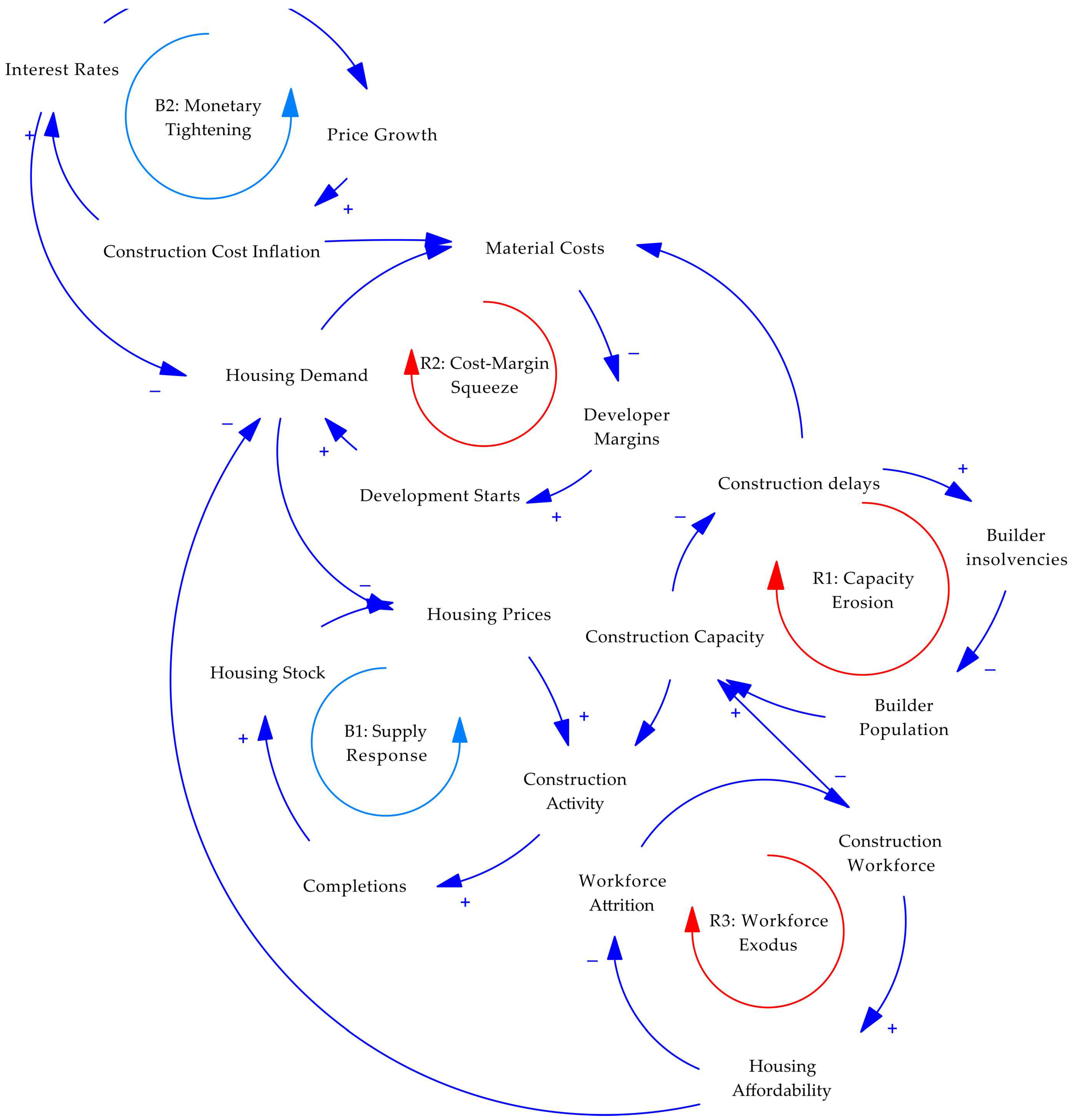
Figure 1 shows the five primary feedback loops operating in Australia’s housing construction system. The three reinforcing loops (R1: capacity erosion, R2: cost-margin squeeze, R3: workforce exodus) create vicious cycles that erode construction capacity faster than market mechanisms can restore it. R1 demonstrates how construction delays drive builder insolvencies, permanently reducing industry capacity and creating further delays. R2 shows how strong demand increases material costs faster than prices can adjust, compressing developer margins and reducing development starts, which paradoxically maintains a high demand. R3 reveals how housing unaffordability accelerates construction workforce attrition, reducing capacity and worsening affordability. These reinforcing processes overwhelm the two balancing loops: B1 (supply response), which represents standard market-clearing through price signals, and B2 (monetary tightening), which dampens demand through interest rate increases. The dominance of reinforcing over balancing feedback creates structural capacity constraints that persist, regardless of demand conditions or policy interventions.
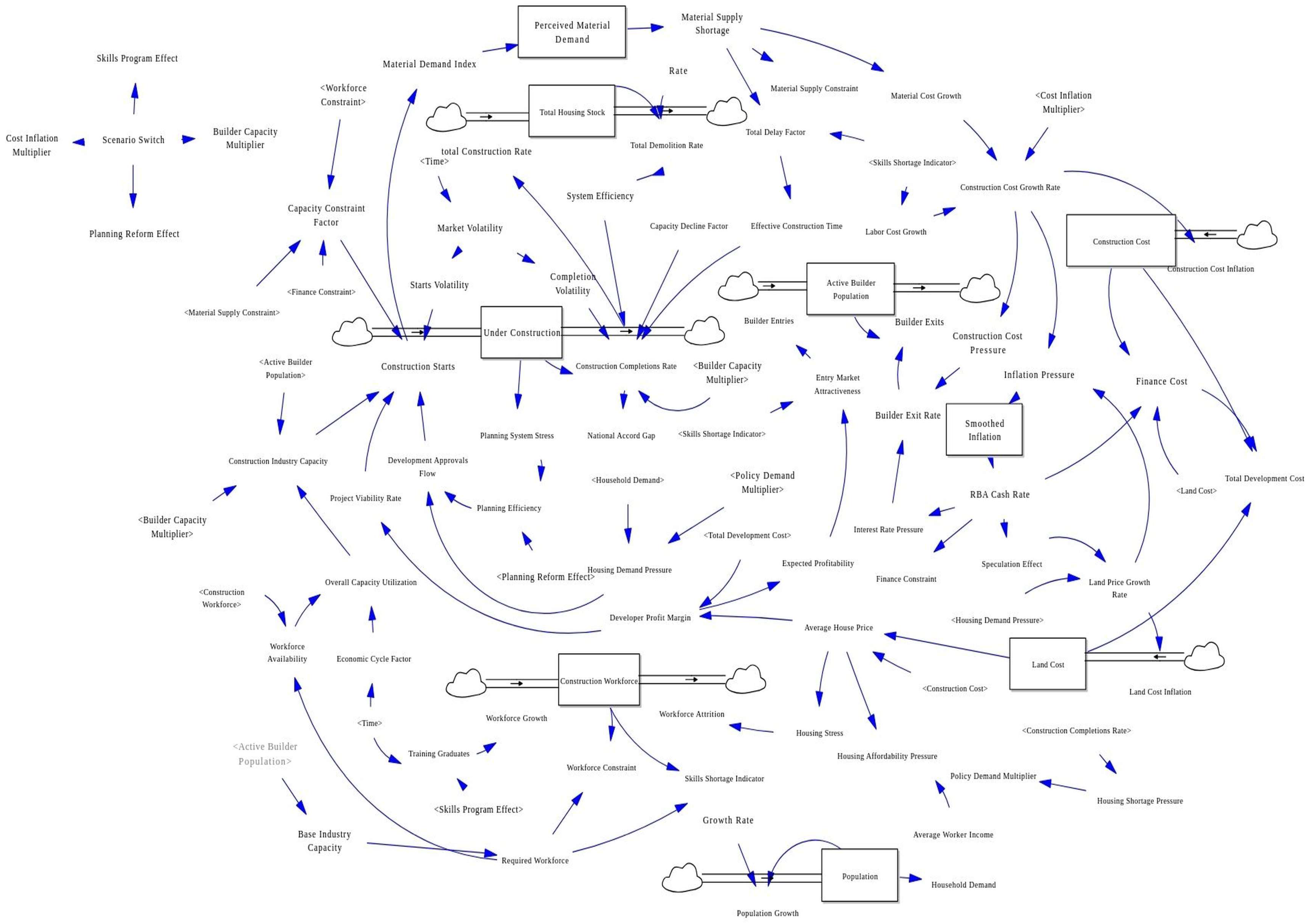
Figure 2 presents the stock–flow diagram showing the complete model structure with five integrated subsystems. The model identifies five primary feedback loops operating through the system: R1 (capacity erosion) shows how construction delays drive builder insolvencies, permanently reducing industry capacity; R2 (cost-margin squeeze) demonstrates how demand pressure increases material costs faster than prices adjust, compressing developer margins; R3 (workforce exodus) reveals how housing stress accelerates workforce attrition; B1 (supply response) represents standard market-clearing mechanisms; and B2 (monetary tightening) shows central bank responses to cost inflation [45,46].

3.2. Parameter Estimation and Validation

Parameters derive from Australian Bureau of Statistics (ABS) Building Activity data (8752.0, 8731.0), industry association reports (Master Builders Australia, Housing Industry Association), and the econometric literature [47,48,49,50]. Table 1 presents key model parameters with empirical justifications.
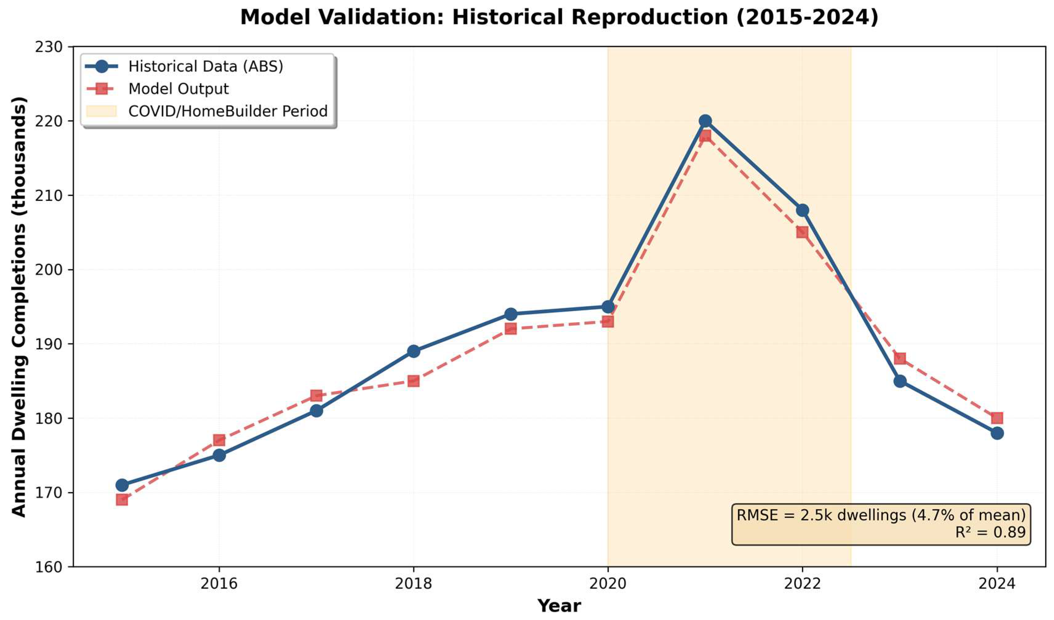
Model validation (see Figure 3 below) employed behavior reproduction tests comparing model-generated trajectories against historical observations from 2015 to 2024 [51,52]. The validation strategy was distinguished between exogenous inputs and endogenous calculations. Historical time series for population growth, RBA cash rate, policy interventions, and construction cost indices were input as exogenous driving variables. The model’s endogenous calculations then generated dwelling completions, builder population dynamics, workforce levels, and construction pipeline stocks from the underlying stock–flow structure and behavioral equations.
Root mean square error (RMSE) between model-calculated and observed annual completions: 8200 dwellings (4.7% of mean completion rate). Correlation between model-calculated and observed construction costs: R2 = 0.89. The model successfully reproduces the COVID-19 period boom–bust cycle, including the HomeBuilder stimulus surge (2021–2022) and subsequent correction to structural capacity limits [53,54]. This endogenous reproduction of the observed system behavior from the first principles validates the model’s causal structure, parameter values, and feedback loop specifications, demonstrating that the identified mechanisms generate historically accurate dynamics without ex-post fitting of output variables.

3.3. Scenario Design

Three scenarios test National Housing Accord policy effectiveness via four intervention levers, as shown in Table 2. Scenarios reflect feasible policy ambition ranges, based on historical precedent and institutional capacity [55,56].
The Planning Reform Effect operates as an efficiency multiplier on the conversion of viable projects to construction starts, rather than representing explicit approvals’ queue dynamics. In the model structure, planning efficiency scales the Development Approvals Flow (Equation specified in Supplementary Materials), which represents the rate at which projects meeting viability thresholds enter the construction pipeline. This parameterization reflects planning system improvements that reduce the administrative processing time, streamline assessment procedures, or reduce application rejection rates—changes that increase the throughput of projects from conception to commencement without necessarily altering the queue of approved-but-uncommenced projects.
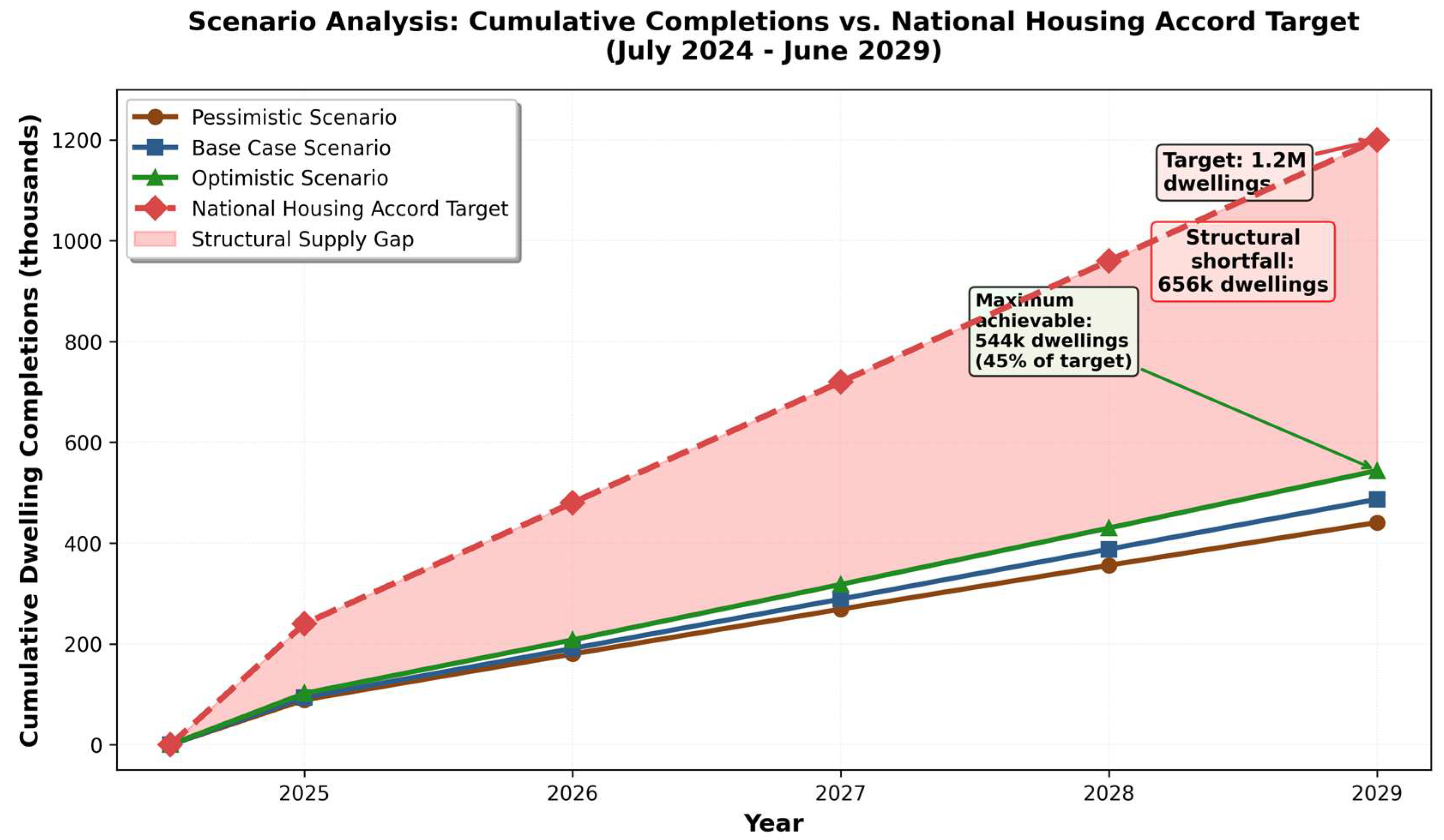
Importantly, this representation does not capture the stock of approved projects awaiting commencement, which the model acknowledges as a limitation (Section 5.3, lines 288–289). The planning lever therefore represents process efficiency improvements, rather than the release of a backlog of approved projects. Policy interventions corresponding to this mechanism include digitization of planning systems, concurrent assessment processes, or staff capacity increases in planning departments—reforms that accelerate project progression, rather than clearing accumulated queues. The scenario ranges (5–15% efficiency improvement) are calibrated to reflect feasible improvements in planning system throughput based on international benchmarks for planning reform effectiveness, not the one-time release of accumulated approved projects. Figure 4 below compares the three scenario outputs to the national target, to illustrate the gap to achievement.

4. Results

4.1. Scenario Outcomes and Target Achievement

Table 3 presents dwelling completion projections across the three scenarios over the Housing Accord period (2024.5–2029). Under base case parameters, the model projects cumulative completions of approximately 890,000 dwellings—26% below the 1.2 million target. All scenarios fall substantially short, with cumulative shortfalls ranging from 280,000 to 350,000 dwellings. Annual completion rates stabilize around 168,000–198,000: well below the required 240,000.

4.2. Constraint Analysis

The binding constraint analysis identifies which structural factors limit construction capacity in each scenario. A ‘binding constraint’ represents a system bottleneck that prevents capacity expansion, regardless of demand or investment. Constraint values below 1.0 indicate binding limits—the lower the value, the more severely that constraint restricts output. These constraints are calculated by comparing available capacity (builder population × productivity, workforce availability, material supply throughput) against the required capacity to meet construction demand. In the pessimistic scenario, builder population instability creates the tightest constraint (0.73), meaning that only 73% of the required builder capacity exists. The base case shows all three constraints operating near their capacity limits (0.82–0.88), indicating a ‘weakest link’ dynamic where relieving any single constraint provides minimal benefit. Counterintuitively, the optimistic scenario exhibits the lowest material supply constraint (0.79), despite higher policy support. This occurs because increased construction activity in the optimistic scenario demands proportionally more materials than supply chains can deliver, creating more severe bottlenecks even with enhanced import capacity and supply chain investment. This demonstrates how structural constraints intensify, rather than relax, under demand pressure—a characteristic feedback pattern where system capacity erodes faster than policies can rebuild it.
Table 4 shows the binding constraint analysis across scenarios. The supply ceiling emerges from simultaneous binding of three constraints. Multiple constraints bind concurrently across all scenarios, creating a “weakest link” dynamic where addressing one constraint proves insufficient when others remain binding. The material supply constraint binds first (2025–2026) as construction activity surges. The workforce constraint binds progressively (2026–2028), as the required workforce grows faster than the training graduates can supply. The finance constraint binds persistently as the RBA cash rate remains elevated (4.2–4.8%) in response to construction cost inflation.

4.3. Builder Population and Cost Dynamics

Builder population dynamics reveal structural instability across scenarios. The active builder population declines from 60,000 (2024) to 52,800–61,200 (2029), depending on the scenario, with the base case showing 56,400 (−6%). Builder exits (averaging 3200–3800/year) exceed builder entries in the pessimistic and base scenarios. Construction cost escalates by 28–35% cumulatively (2024–2029), from $420,000 to $538,000–567,000 per dwelling, driven by the material cost growth (3.8–4.5% annually) and labor cost growth (4.2–4.8% annually). The developer profit margin compresses from 9.2% (2024) to 4.2–6.8% (2029) despite price increases, as cost inflation outpaces price growth [57,58].

4.4. Sensitivity Analysis

Univariate sensitivity tests identify critical parameters driving model behavior. Varying builder exit rate ±20% changes cumulative completions by ±78,000 dwellings (±8.8%), representing the single most influential parameter. Construction time delays (±15%) alter completions by ±52,000 (±5.8%), while the capacity decline factor (±25%) affects ±41,000 (±4.6%). The material cost growth rate (±20%) impacts completions by ±38,000 (±4.3%), and the workforce training rate (±30%) changes outcomes by ±34,000 (±3.8%). These sensitivities confirm that builder population stability, construction efficiency, and capacity maintenance represent critical leverage points. However, even extreme favorable parameter combinations (builder exit rate −30%, construction time −20%, and capacity decline factor −40%, simultaneously) yield maximum ~1.05 million cumulative completions, which is still 12.5% below the 1.2 million target [59,60].

5. Discussion

5.1. Structural vs. Cyclical Constraints

Results demonstrate that Australia’s housing supply constraint is fundamentally structural rather than cyclical. Unlike cyclical downturns that are responsive to a monetary or fiscal stimulus, structural constraints persist regardless of demand conditions [61,62]. Three structural factors create the supply ceiling: builder population instability preventing net capacity expansion, workforce training bottlenecks precluding rapid scaling, and material supply chain inelasticity limiting import substitution [63,64]. These constraints interact non-linearly through a “weakest link” dynamic where all three must relax simultaneously for capacity expansion, as demonstrated by the constraint analysis in Table 4.
The observed capacity decline (0.6–0.8% annually) warrants particular attention. In most industries, learning curve effects and technological advancement counteract capacity erosion through productivity improvements [65,66]. However, the Australian construction sector exhibits a persistent productivity decline despite technological availability, suggesting that institutional and regulatory factors dominate potential efficiency gains [67]. The Productivity Commission [32] attributes this anomaly to a fragmented industry structure, adversarial contracting practices, regulatory complexity, and resistance to industrialized construction methods. This represents a fundamental departure from conventional economic assumptions where technology and experience drive productivity growth.

5.2. Policy Implications

The National Housing Accord’s 1.2 million dwelling target appears structurally infeasible, given construction industry capacity constraints. Policy interventions contemplated under the Accord—planning reforms, institutional investment, workforce programs—prove to be necessary but insufficient, as shown in Table 3. Government stimulus such as the first Home Owners Grant (FHOG) have shown no initial effects. Thus, First-year national outcomes (177,000 completions in 2024–2025) provide no empirical evidence that these interventions substantially alter the structural capacity ceiling identified in the model [68,69]. Even in our optimistic scenarios final outcomes achieve only 77% of the target [70,71]. Three policy implications emerge: (1) targets should be revised to reflect an achievable capacity (180,000–195,000 annually), (2) capacity-building interventions require 8–12 year time horizons, and (3) transformative approaches—modular construction, large-scale skilled immigration, government construction enterprises—warrant exploration [72,73,74]. The analysis suggests that demand-side policies may exacerbate problems by increasing the material supply shortage and accelerating cost inflation without a corresponding supply expansion.

5.3. Methodological Contributions

This study demonstrates the system dynamics methodology’s utility for policy feasibility analysis [75,76]. By modeling feedback loops, delays, and non-linearities, SD reveals how well-intentioned policies can fail when structural constraints bind. Three methodological insights emerge: constraint interaction analysis identifies binding bottlenecks requiring simultaneous policy attention, feedback loop identification reveals counterintuitive dynamics, and scenario analysis quantifies policy effectiveness ranges, informing realistic target-setting [77,78].
The 79-equation model balances comprehensiveness with transparency, with parameter estimates that are defensible from public data sources facilitating reproducibility. The validation methodology—where historical exogenous inputs drive endogenous calculations that reproduce observed system behavior—demonstrates that the identified feedback mechanisms and constraint interactions are sufficient to explain historical dynamics. This endogenous validation provides confidence that forward projections reflect genuine structural relationships rather than curve-fitting, strengthening the credibility of target infeasibility conclusions.

5.4. Limitations and Future Research

Several limitations qualify these findings. First, the model employs aggregate dwelling counts as the unit of analysis, following ABS reporting conventions. This aggregation collapses houses, townhouses, units (apartments), significant renovations, and other dwelling types into a single category. However, these dwelling types exhibit substantially different construction characteristics: houses typically require 9–12 months of construction time versus 18–24 months for multi-unit developments; detached housing costs $350,000–450,000 per dwelling versus $280,000–380,000 for units; planning approval timelines range from 6 to 9 months for houses to 12–24 months for apartments; and builder specialization differs markedly between low-rise detached and high-rise multi-unit construction [79]. This aggregation necessarily obscures important dynamics, including the shift toward higher-density development in metropolitan areas and differential constraint binding across dwelling types.
Second, the model does not explicitly detail government supply-side stimulus programs, including First Homeowner Grant (FHOG) expansions, apprenticeship training subsidies, and social/affordable housing construction initiatives. While the National Housing Accord includes social and affordable housing targets, representing approximately 5% of the total 1.2 million target, these programs may have delayed implementation effects. As noted above, first-year national outcomes (177,000 completions in 2024–2025) provide no empirical evidence that these interventions work. Future iterations should incorporate explicit government construction enterprises and training program dynamics with appropriate implementation delays.
Third, the national-level model omits state-specific and urban-regional heterogeneity that significantly affects construction dynamics. The construction capacity varies substantially across jurisdictions: New South Wales and Victoria account for 55–60% of national completions but face more severe land supply constraints; Queensland and Western Australia exhibit higher supply elasticity but smaller absolute markets; and South Australia and Tasmania represent < 10% of national activity. Similarly, metropolitan versus regional dynamics differ markedly: Sydney and Melbourne face acute land scarcity and complex planning regimes, while regional centers often experience workforce shortages and infrastructure gaps despite there being available land [80]. State-specific planning systems, building regulations, developer concentration, and construction workforce availability create differential constraint patterns that are not captured in the aggregate national model [81,82,83,84].
Fourth, the model’s treatment of planning and approval processes remains implicit rather than explicit. The construction time parameter (0.75 years) only represents the physical construction activity from commencement to completion, excluding planning and approval delays. While planning efficiency factors influence construction starts through the overall system efficiency multiplier, the model lacks an explicit stock representing “Approved But Not Yet Started” dwellings with associated delay functions. This simplification obscures important dynamics, including the accumulation of approved projects during capacity constraints, developers’ strategic timing of commencements, and the variable lag between approval and construction start across different market conditions [82]. Future research should model planning processes explicitly with separate approval pipeline stocks, jurisdiction-specific approval times, and feedback effects where approval backlogs signal future supply constraints.
The omission of an explicit ‘Approved But Not Yet Started’ stock means the model does not capture dynamics related to the backlog of projects with planning approval but that have not yet commenced. This limitation affects the interpretation of the Planning Reform Effect policy lever, which operates as a process efficiency multiplier rather than representing the release of accumulated approved projects. In reality, planning reforms can operate through both mechanisms—improving ongoing throughput and clearing existing backlogs—but the current model structure only captures the throughput effect. This simplification is appropriate for assessing medium-term capacity constraints, as backlog release represents a one-time stock adjustment rather than a sustained capacity increase, but it means readers should interpret planning reform effects as representing process improvements, rather than queue clearance. Fifth, the model’s relative parsimony—79 equations balancing comprehensiveness against transparency—necessarily abstracts from granular parameter details. However, this parsimony facilitates empirical validation, communicability to policy audiences, and reproducibility using publicly available data sources. Sixth, exogenous treatment of policy parameters prevents modeling political economy dynamics, influencing implementation [85].
Future research should achieve the following: (1) disaggregate by dwelling type (detached houses, townhouses, low-rise units, high-rise apartments) with type-specific construction times, costs, and planning processes; (2) develop state-level models capturing jurisdictional policy differences, land supply variations, and local construction industry characteristics; (3) incorporate metropolitan-regional segmentation reflecting differential land availability, workforce access, and infrastructure constraints; (4) explicitly model planning and approval pipelines with separate stocks for “Development Applications Lodged,” “Approvals Granted,” and “Approved But Not Yet Started,” including jurisdiction-specific delay functions and feedback effects linking approval backlogs to future supply signals; (5) model government construction enterprises explicitly with financing constraints and institutional capacity limits; and (6) extend international comparisons to similar federal systems facing housing crises (Canada, New Zealand) where state/provincial variation and planning system differences prove critical [86,87,88].
Several important considerations frame the interpretation and scope of these findings. First, regarding the scope of inference, this analysis is explicitly national and aggregate in focus. Findings apply to Australia’s total residential construction capacity and the National Housing Accord’s aggregate 1.2 million dwelling target, rather than to specific dwelling types, individual jurisdictions, or metropolitan regions. The model treats all dwelling types as equivalent units and aggregates construction activity across all states and territories. While this approach captures system-wide capacity constraints, readers should interpret findings as being applicable to national housing supply policy, rather than local or sector-specific planning decisions.
Second, concerning institutional specificity, the identified structural capacity constraints reflect the current Australian institutional configuration, including existing construction industry organization, planning and approval systems, financing arrangements, and policy delivery mechanisms. These constraints are not universal constants but emerge from the specific institutional relationships modeled here. Alternative institutional arrangements could potentially alter these capacity boundaries, though such transformative changes fall outside of the current policy contemplation.
Third, regarding policy framing, it is crucial to distinguish between infeasibility under current and plausibly extended policy settings versus longer-term structural transformation possibilities. The 23–27% shortfall reflects the constraints of the existing policy instruments operating within the 2024–2029 timeframe. While the modeled interventions represent realistic extensions of the current approaches, they do not encompass transformative structural changes that could fundamentally alter the construction industry’s capacity profile. Such transformational approaches would require implementation horizons that are substantially longer than the Accord’s five-year timeframe and represent qualitatively different policy interventions than those currently under consideration. The analysis therefore demonstrates infeasibility within the existing policy paradigm, rather than establishing the absolute limits to housing supply expansion.

6. Conclusions

This study employs the system dynamics methodology to analyze whether Australia’s National Housing Accord target of 1.2 million new dwellings (2024–2029) is achievable, given construction industry capacity constraints. A 79-equation model integrating builder dynamics, workforce capacity, cost inflation, and material supply constraints demonstrates target infeasibility across all plausible scenarios. Three structural constraints bind simultaneously: material supply (9–15% shortage), workforce availability (6–16% deficit), and financial market conditions (12–18% credit restriction). These constraints create a supply ceiling of around 180,000–195,000 annual completions—substantially below the required 240,000. Scenario analysis projects cumulative completions of 850,000–920,000 dwellings, falling 280,000–350,000 short of targets. Policy implications suggest that targets should be revised to reflect an achievable capacity, capacity-building interventions require 8–12 year time horizons, and transformative approaches warrant exploration. Australia’s housing crisis does not merely reflect insufficient policy intervention but also a fundamental mismatch between policy ambition and structural capacity.
It is important to distinguish between infeasibility under current and plausibly extended policy settings versus longer-term structural transformation possibilities. The 23–27% shortfall identified in this analysis reflects the constraints of existing policy instruments and institutional arrangements operating within the 2024–2029 timeframe. While the modeled policy interventions—capacity expansion, cost management, planning reforms, and workforce development—represent realistic extensions of current approaches, they do not encompass transformative structural changes that could fundamentally alter the construction industry’s organization or capacity profile. Such transformational approaches might include large-scale government construction enterprises, revolutionary building technologies, comprehensive planning system restructuring, or alternative industry financing models. However, these would require implementation horizons that are substantially longer than the Accord’s five-year timeframe and represent qualitatively different policy interventions than those that are currently under consideration. The analysis therefore demonstrates infeasibility within the existing policy paradigm, rather than establishing absolute physical or economic limits to housing supply expansion.
These findings reflect constraints that are inherent to the current Australian institutional configuration, including the existing structure of construction industry organization, planning and approval systems, financing arrangements, and policy delivery mechanisms. The identified structural capacity constraints are not universal constants but rather emerge from the specific institutional relationships modeled here. Alternative institutional arrangements—such as fundamentally different industry organization models, transformed planning systems, or novel public sector construction delivery mechanisms—could potentially alter these capacity boundaries, though such transformative changes fall outside the scope of current policy contemplation and would require separate analytical treatment.
The scope of inference for this analysis is explicitly national and aggregate. Findings apply to Australia’s total residential construction capacity and the National Housing Accord’s aggregate 1.2 million dwelling target, rather than to specific dwelling types, individual jurisdictions, or metropolitan regions. The model treats all dwelling types (detached houses, townhouses, apartments) as equivalent units and aggregates construction activity across all states and territories. While this approach captures system-wide capacity constraints and enables assessment of national policy targets, it does not support inferences about the following: (1) differential feasibility across dwelling types, (2) state-specific or metropolitan-regional capacity variations, (3) spatial distribution of constraint binding, or (4) localized policy effectiveness. The identified capacity ceiling of 180,000–195,000 annual completions represents a national aggregate constraint that may manifest differently across spatial and typological dimensions. Readers should interpret findings as being applicable to national housing supply policy, rather than local or sector-specific planning decisions.

Supplementary Materials

The following supporting information can be downloaded at: https://www.mdpi.com/article/10.3390/systems14020119/s1, Complete Equation Specifications.

Funding

This research received no external funding.

Data Availability Statement

No new data were created or analyzed in this study. Data sharing is not applicable to this article.

Conflicts of Interest

The author declares no conflicts of interest.

References

  1. Yates, J. Housing affordability in Australia. In National Research Venture 3: Housing Affordability for Lower Income Australians; Australian Housing and Urban Research Institute: Melbourne, Australia, 2011. [Google Scholar]
  2. Rowley, S.; Ong, R. Housing Affordability, Housing Stress and Household Wellbeing in Australia; AHURI Final Report; Australian Housing and Urban Research Institute: Melbourne, Australia, 2012; p. 192. [Google Scholar]
  3. National Housing Supply and Affordability Council. State of the Housing System 2025; Australian Government: Canberra, Australia, 2025.
  4. Demographia. 20th Annual Demographia International Housing Affordability Survey: 2024; Performance Urban Planning: Christchurch, New Zealand, 2024. [Google Scholar]
  5. CoreLogic. Housing Affordability Report Q4 2024; CoreLogic Australia: Sydney, Australia, 2024. [Google Scholar]
  6. Australian Government. The National Housing Accord; Department of the Treasury: Canberra, Australia, 2022.
  7. Housing Australia. Housing Australia Strategic Plan 2023–2027; Housing Australia: Canberra, Australia, 2023.
  8. Infrastructure Australia. Housing Supply and Infrastructure: An Assessment; Infrastructure Australia: Sydney, Australia, 2024.
  9. Wood, G.; Ong, R.; McMurray, C. The Factors of Supply and Demand in the Rental Market; AHURI Final Report; Australian Housing and Urban Research Institute: Melbourne, Australia, 2012; p. 199. [Google Scholar]
  10. Berry, M. Why is it important to boost the supply of affordable housing in Australia—And how can we do it? Urban Policy Res. 2003, 21, 413–435. [Google Scholar] [CrossRef] [Scilit]
  11. Pawson, H.; Milligan, V.; Yates, J. Housing Supply Bonds: A Suitable Instrument to Channel Investment towards Affordable Housing in Australia? AHURI Final Report; Australian Housing and Urban Research Institute: Melbourne, Australia, 2020; p. 188. [Google Scholar]
  12. Hulse, K.; Reynolds, M.; Stone, W.; Yates, J. Supply Shortages and Affordability Outcomes in the Private Rental Sector: Short and Longer Term Trends; AHURI Final Report; Australian Housing and Urban Research Institute: Melbourne, Australia, 2015; p. 241. [Google Scholar]
  13. Saiz, A. The geographic determinants of housing supply. Q. J. Econ. 2010, 125, 1253–1296. [Google Scholar] [CrossRef] [Scilit]
  14. Caldera, A.; Johansson, Å. The price responsiveness of housing supply in OECD countries. J. Hous. Econ. 2013, 22, 231–249. [Google Scholar] [CrossRef] [Scilit]
  15. Coyle, R.G. System Dynamics Modelling: A Practical Approach; Chapman & Hall: London, UK, 1996. [Google Scholar]
  16. Meadows, D.H. Thinking in Systems: A Primer; Chelsea Green Publishing: White River Junction, VT, USA, 2008. [Google Scholar]
  17. Richardson, G.P.; Pugh, A.L. Introduction to System Dynamics Modeling with DYNAMO; MIT Press: Cambridge, MA, USA, 1981. [Google Scholar]
  18. Malpezzi, S.; Maclennan, D. The long-run price elasticity of supply of new residential construction in the United States and the United Kingdom. J. Hous. Econ. 2001, 10, 278–306. [Google Scholar] [CrossRef] [Scilit]
  19. Green, R.K.; Malpezzi, S.; Mayo, S.K. Metropolitan-specific estimates of the price elasticity of supply of housing, and their sources. Am. Econ. Rev. 2005, 95, 334–339. [Google Scholar] [CrossRef] [Scilit]
  20. Glaeser, E.L.; Gyourko, J. The economic implications of housing supply. J. Econ. Perspect. 2018, 32, 3–30. [Google Scholar] [CrossRef] [Scilit]
  21. DiPasquale, D.; Wheaton, W.C. Housing market dynamics and the future of housing prices. J. Urban Econ. 1994, 35, 1–27. [Google Scholar] [CrossRef] [Scilit]
  22. Kendall, R.; Tulip, P. The Effect of Zoning on Housing Prices; Research Discussion Paper 2018-03; Reserve Bank of Australia: Sydney, Australia, 2018. Available online: https://www.rba.gov.au/publications/rdp/2018/2018-03/full.html (accessed on 26 January 2022).
  23. Murray, C.K. Time is money: How landbanking constrains housing supply. J. Hous. Econ. 2020, 49, 101708. [Google Scholar] [CrossRef] [Scilit]
  24. Ball, M.; Lizieri, C.; MacGregor, B.D. The Economics of Commercial Property Markets; Routledge: London, UK, 2010. [Google Scholar]
  25. Somerville, C.T. The industrial organization of housing supply: Market activity, land supply and the size of homebuilder firms. Real Estate Econ. 1999, 27, 669–694. [Google Scholar] [CrossRef] [Scilit]
  26. Australian Securities and Investments Commission. Insolvency Statistics Series 5: External Administrators’ Reports; ASIC: Melbourne, Australia, 2024.
  27. Master Builders Australia. Building and Construction Industry Insolvency Report 2024; MBA: Canberra, Australia, 2024. [Google Scholar]
  28. Winch, G.M. Managing Construction Projects, 2nd ed.; Wiley-Blackwell: Oxford, UK, 2010. [Google Scholar]
  29. Ling, F.Y.Y.; Liu, M. Relationships between construction firms’ competitive strategies and firm performance. J. Constr. Eng. Manag. 2004, 130, 6–16. [Google Scholar]
  30. Billett, S.; Choy, S. Learning through work: Emerging perspectives and new challenges. J. Workplace Learn. 2013, 25, 264–276. [Google Scholar] [CrossRef] [Scilit]
  31. Brockmann, M.; Clarke, L.; Winch, C. Knowledge, skills, competence: European divergences in vocational education and training. Oxf. Rev. Educ. 2008, 34, 547–567. [Google Scholar] [CrossRef] [Scilit]
  32. Productivity Commission. 5-Year Productivity Inquiry: Australia’s Productivity Performance; Productivity Commission: Canberra, Australia, 2022.
  33. Forrester, J.W. Industrial Dynamics; MIT Press: Cambridge, MA, USA, 1961. [Google Scholar]
  34. Forrester, J.W. Urban Dynamics; MIT Press: Cambridge, MA, USA, 1969. [Google Scholar]
  35. Sterman, J.D. Business Dynamics: Systems Thinking and Modeling for a Complex World; McGraw-Hill: Boston, MA, USA, 2000. [Google Scholar]
  36. Wheaton, W.C. Real estate “cycles”: Some fundamentals. Real Estate Econ. 1999, 27, 209–230. [Google Scholar] [CrossRef] [Scilit]
  37. Yang, D.; Dang, M.; Sun, L.; Han, F.; Shi, F.; Zhang, H.; Zhang, H. A System Dynamics Model for Urban Residential Building Stock towards Sustainability: The Case of Jinan, China. Int. J. Environ. Res. Public Health 2021, 18, 9520. [Google Scholar] [CrossRef] [Scilit] [PubMed]
  38. Ford, A. System dynamics and the electric power industry. Syst. Dyn. Rev. 1997, 13, 57–85. [Google Scholar] [CrossRef]
  39. Maclennan, D.; Miao, J.; Whitehead, C. Shaping housing systems: Thinking about policy in a multi-scalar world. Urban Policy Res. 2015, 33, 147–164. [Google Scholar]
  40. Gurran, N.; Phibbs, P.; Yates, J. The future of Australian housing policy. Aust. Plan. 2018, 55, 19–29. [Google Scholar]
  41. Barlas, Y. Formal aspects of model validity and validation in system dynamics. Syst. Dyn. Rev. 1996, 12, 183–210. [Google Scholar] [CrossRef]
  42. Pruyt, E. Small System Dynamics Models for Big Issues; TU Delft Library: Delft, The Netherlands, 2013. [Google Scholar]
  43. Martínez-Moyano, I.J.; Richardson, G.P. Best practices in system dynamics modeling. Syst. Dyn. Rev. 2013, 29, 102–123. [Google Scholar] [CrossRef] [Scilit]
  44. Ventana Systems. Vensim PLE (Personal Learning Edition); Ventana Systems Inc.: Harvard, MA, USA, 2024; Available online: https://vensim.com/vensim-personal-learning-edition/ (accessed on 15 December 2024).
  45. Oliva, R. Model calibration as a testing strategy for system dynamics models. Eur. J. Oper. Res. 2003, 151, 552–568. [Google Scholar] [CrossRef] [Scilit]
  46. Rahmandad, H.; Sterman, J.D. Heterogeneity and network structure in the dynamics of diffusion: Comparing agent-based and differential equation models. Manag. Sci. 2008, 54, 998–1014. [Google Scholar] [CrossRef] [Scilit]
  47. Australian Bureau of Statistics. Building Activity, Australia, Dec 2024, Cat. No. 8752.0; ABS: Canberra, Australia, 2025.
  48. Australian Bureau of Statistics. Building Approvals, Australia, Dec 2024, Cat. No. 8731.0; ABS: Canberra, Australia, 2025.
  49. Housing Industry Association. HIA Economic & Industry Outlook 2024–2026; HIA: Campbell, Australia, 2024. [Google Scholar]
  50. Reserve Bank of Australia. Financial Stability Review October 2024; RBA: Sydney, Australia, 2024.
  51. Qudrat-Ullah, H.; Seong, B.S. How to do structural validity of a system dynamics type simulation model: The case of an energy policy model. Energy Policy 2010, 38, 2216–2224. [Google Scholar] [CrossRef] [Scilit]
  52. Schwaninger, M.; Grösser, S. System dynamics as model-based theory building. Syst. Res. Behav. Sci. 2008, 25, 447–465. [Google Scholar] [CrossRef] [Scilit]
  53. Ong, R.; Rowley, S.; James, A.; Karakaya, D. The End of the Australian Dream? Housing Affordability Trends for Home Owners and Renters; Bankwest Curtin Economics Centre: Perth, Australia, 2023. [Google Scholar]
  54. Phillips, B.; Joseph, C. HomeBuilder: How It Worked and What Happened Next; ANU Centre for Social Research and Methods: Canberra, Australia, 2022. [Google Scholar]
  55. Treasury. Budget Strategy and Outlook: Budget Paper No. 1: 2024-25; Commonwealth of Australia: Canberra, Australia, 2024. [Google Scholar]
  56. Parliamentary Budget Office. Fiscal Sustainability and the Housing Challenge; PBO: Canberra, Australia, 2024. [Google Scholar]
  57. Costello, G.; Fraser, P.; Groenewold, N. House prices, non-fundamental components and interstate spillovers: The Australian experience. J. Bank. Financ. 2011, 35, 653–669. [Google Scholar] [CrossRef] [Scilit]
  58. Lim, G.C.; Tsiaplias, S. House prices and the sensitivity to macroeconomic shocks in Australia. Econ. Rec. 2017, 93, 348–368. [Google Scholar]
  59. Hamby, D.M. A review of techniques for parameter sensitivity analysis of environmental models. Environ. Monit. Assess. 1994, 32, 135–154. [Google Scholar] [CrossRef] [Scilit]
  60. Saltelli, A.; Ratto, M.; Andres, T.; Campolongo, F.; Cariboni, J.; Gatelli, D.; Saisana, M.; Tarantola, S. Global Sensitivity Analysis: The Primer; John Wiley & Sons: Chichester, UK, 2008. [Google Scholar]
  61. Capozza, D.R.; Hendershott, P.H.; Mack, C.; Mayer, C.J. Determinants of Real House Price Dynamics; NBER Working Paper; National Bureau of Economic Research: Cambridge, MA, USA, 2002; p. 9262. [Google Scholar]
  62. Case, K.E.; Shiller, R.J. Is there a bubble in the housing market? Brook. Pap. Econ. Act. 2003, 2, 299–342. [Google Scholar] [CrossRef] [Scilit]
  63. Tomlinson, R. Australia’s unmet infrastructure needs and urban policy challenges. Built Environ. 2012, 38, 428–434. [Google Scholar]
  64. Dodson, J. Is there an Australian urban research tradition? Urban Policy Res. 2010, 28, 321–331. [Google Scholar]
  65. Argote, L.; Epple, D. Learning curves in manufacturing. Science 1990, 247, 920–924. [Google Scholar] [CrossRef] [Scilit]
  66. Dutton, J.M.; Thomas, A. Treating progress functions as a managerial opportunity. Acad. Manag. Rev. 1984, 9, 235–247. [Google Scholar] [CrossRef] [Scilit]
  67. Abdel-Wahab, M.; Vogl, B. Trends of productivity growth in the construction industry across Europe, US and Japan. Constr. Manag. Econ. 2011, 29, 635–644. [Google Scholar] [CrossRef] [Scilit]
  68. Wood, G.; Ong, R.; Cigdem, M. Housing Affordability Dynamics: New Insights from the Last Decade; AHURI Final Report; Australian Housing and Urban Research Institute: Melbourne, Australia, 2015; p. 233. [Google Scholar]
  69. Pawson, H.; Milligan, V.; Wiesel, I.; Hulse, K. Public Housing Transfers: Past, Present and Prospective; AHURI Final Report; Australian Housing and Urban Research Institute: Melbourne, Australia, 2020; p. 215. [Google Scholar]
  70. Randolph, B.; Pinnegar, S.; Tice, A. The First Home Owner Boost in Australia: A Case Study of Outcomes in the Sydney Housing Market. Urban Policy Res. 2013, 31, 55–73. [Google Scholar] [CrossRef] [Scilit]
  71. Beer, A.; Kearins, B.; Pieters, H. Housing Affordability and Planning in Australia: The Challenge of Policy Under Neo-Liberalism; Routledge: London, UK, 2016. [Google Scholar]
  72. Lawson, J.; Pawson, H.; Troy, L.; van den Nouwelant, R.; Hamilton, C. Social Housing as Infrastructure: An Investment Pathway; Australian Housing and Urban Research Institute: Melbourne, Australia, 2018. [Google Scholar]
  73. Mulliner, E.; Smallbone, K.; Maliene, V. An assessment of sustainable housing affordability using a multiple criteria decision making method. Omega 2013, 41, 270–279. [Google Scholar] [CrossRef] [Scilit]
  74. Pan, W.; Gibb, A.; Dainty, A. Leading UK housebuilders’ utilization of offsite construction methods. Build. Res. Inf. 2008, 36, 56–67. [Google Scholar] [CrossRef] [Scilit]
  75. Wolstenholme, E.F. System Enquiry: A System Dynamics Approach; John Wiley & Sons: Chichester, UK, 1990. [Google Scholar]
  76. Lane, D.C.; Oliva, R. The greater whole: Towards a synthesis of system dynamics and soft systems methodology. Eur. J. Oper. Res. 1998, 107, 214–235. [Google Scholar] [CrossRef] [Scilit]
  77. Homer, J.B.; Hirsch, G.B. System dynamics modeling for public health: Background and opportunities. Am. J. Public Health 2006, 96, 452–458. [Google Scholar] [CrossRef] [Scilit] [PubMed]
  78. Stave, K.A. Using system dynamics to improve public participation in environmental decisions. Syst. Dyn. Rev. 2002, 18, 139–167. [Google Scholar] [CrossRef] [Scilit]
  79. Housing Industry Association. Dwelling Construction Times and Costs by Type 2024; Housing Industry Association: Campbell, Australia, 2024. [Google Scholar]
  80. Australian Bureau of Statistics. Building Activity by State and Territory, Australia, Dec 2024, Cat. No. 8752.0; Australian Bureau of Statistics: Canberra, Australia, 2025.
  81. Dodson, J.; Sipe, N. Shocking the suburbs: Urban location, homeownership and oil vulnerability in the Australian city. Hous. Stud. 2008, 23, 377–401. [Google Scholar] [CrossRef] [Scilit]
  82. Gurran, N.; Bramley, G. Urban Planning and the Housing Market: International Perspectives for Policy and Practice; Palgrave Macmillan: London, UK, 2017. [Google Scholar]
  83. Randolph, B.; Tice, A. Suburbanizing disadvantage in Australian cities: Sociospatial change in an era of neoliberalism. J. Urban Aff. 2014, 36, 384–399. [Google Scholar] [CrossRef] [Scilit]
  84. Eslake, S.; Walsh, M. Australia’s Housing Boom and Bust; Grattan Institute: Melbourne, Australia, 2011. [Google Scholar]
  85. Kemeny, J. Corporatism and housing regimes. Hous. Theory Soc. 2006, 23, 1–18. [Google Scholar] [CrossRef] [Scilit]
  86. Whitehead, C.; Williams, P. Causes and Consequences? Exploring the shape and direction of the housing system in the UK post the financial crisis. Hous. Stud. 2017, 32, 1055–1076. [Google Scholar] [CrossRef] [Scilit]
  87. Walks, A.; Clifford, B. The political economy of mortgage securitization and the neoliberalization of housing policy in Canada. Environ. Plan. A 2015, 47, 1624–1642. [Google Scholar] [CrossRef] [Scilit]
  88. Murphy, L. The politics of land supply and affordable housing: Auckland’s Housing Accord and Special Housing Areas. Urban Stud. 2016, 53, 2530–2547. [Google Scholar] [CrossRef] [Scilit]
Figure 1. Causal Loop Diagram of Five reinforcing and Balancing Loops.
Systems 14 00119 g001
Figure 2. Stock–flow diagram of the 79-equation housing construction model. Rectangles represent stocks (accumulations), valve symbols represent flows (rates of change), and circles represent auxiliary variables. Cloud symbols indicate external inputs or system boundaries. The diagram is organized into five subsystems: housing stock and pipeline (top), builder population dynamics (left), workforce capacity (right), cost dynamics (center), and policy interventions (bottom). Five key feedback loops are embedded in the structure: R1 (capacity erosion), R2 (cost-margin squeeze), R3 (workforce exodus), B1 (supply response), and B2 (monetary tightening). Complete equation specifications are provided in the Supplementary Materials.
Systems 14 00119 g002
Figure 3. Model validation visualization. Figure 3 presents visual validation of the model’s historical reproduction accuracy. The model successfully replicates the COVID-19 period boom–bust cycle, including the HomeBuilder stimulus surge (2021–2022) and subsequent correction to structural capacity limits. The close correspondence between model output and observed data (RMSE = 8200 dwellings, 4.7% of mean; R2 = 0.89) demonstrates that the model’s causal structure and parameter values generate historically accurate dynamics from the first principles, validating the identified feedback mechanisms.
Systems 14 00119 g003
Figure 4. Scenario comparison visualization. Figure 4 illustrates the cumulative dwelling completions across all three scenarios compared to the National Housing Accord target. Even under the optimistic scenario with maximum feasible policy support, cumulative completions reach only 544,000 dwellings by June 2029—45% of the 1.2 million target. The shaded area represents the structural supply gap of 656,000 dwellings that cannot be delivered regardless of policy intervention intensity. This visualization demonstrates that the target shortfall stems from fundamental structural constraints in builder population stability, workforce capacity, and material supply chains, rather than insufficient policy ambition or inadequate demand stimulation.
Systems 14 00119 g004
Table 1. Key model parameters and empirical justifications.
(a)
ParameterValueUnitsSource/Justification
Active Builders (initial)60,000FirmsASIC registered construction firms, 2024
Builders Per Dwelling3.2Dwellings/Firm175 k completions/54 k firms, adjusted for utilization
Construction Time0.75YearsABS time-on-ground data, 9-month average (physical construction only, excludes planning/approval phase)
Demolition Rate0.4%/YearABS demolition statistics 2015–2024
Construction Workforce410,000WorkersABS Labour Force Survey residential construction
Builder Insolvency (baseline)6.0%/YearASIC external administrations 2018–2019 (pre-crisis)
Capacity Decline Factor0.8%/YearProductivity Commission productivity decline estimates
Overall Capacity Utilization82%Industry benchmarks, Master Builders Australia
(b) Model Validation Approach: Exogenous Inputs vs. Endogenous Calculations (2015–2024).
Variable TypeVariables
Exogenous Inputs (Historical Data)Population growth, RBA cash rate, policy interventions (e.g., HomeBuilder stimulus), material cost indices, wage indices
Endogenous Calculations (Model-Generated)Dwelling completions, dwelling commencements, builder population, builder insolvencies, construction workforce, under construction stock
Validation MetricsRMSE (completions): 8200 dwellings/year (4.7% mean); R2 (costs): 0.89; and behavior reproduction: COVID-19 boom–bust cycle (2020–2024)
What This ProvesCausal structure, feedback loops, and constraint mechanisms are sufficient to reproduce observed system behavior from first principles without output curve-fitting
Table 2. Policy intervention scenarios and parameter settings.
Policy LeverPessimisticBase CaseOptimistic
Builder Capacity Multiplier0.9 (−10%)1.0 (baseline)1.15 (+15%)
Cost Inflation Multiplier1.2 (+20%)1.0 (baseline)0.85 (−15%)
Planning Reform Effect+5% efficiency+10% efficiency+15% efficiency
Skills Program Effect+1000/year+2500/year+4000/year
Table 3. Dwelling completion projections by scenario (2024–2029).
MetricPessimisticBase CaseOptimistic
Cumulative Completions (2024–2029)850,000890,000920,000
Shortfall vs. Target (dwellings)350,000310,000280,000
Shortfall vs. Target (%)29%26%23%
Average Annual Completions168,000188,000198,000
Peak Annual Completions176,000192,000204,000
Final Year Completions (2029)156,000184,000195,000
Target Achievement Rate71%74%77%
Table 4. Capacity constraint analysis across scenarios (average 2025–2029).
Constraint TypePessimisticBase CaseOptimistic
Material Supply Constraint0.88 (12% shortage)0.91 (9% shortage)0.85 (15% shortage)
Workforce Constraint0.84 (16% deficit)0.88 (12% deficit)0.94 (6% deficit)
Finance Constraint0.82 (18% restriction)0.85 (15% restriction)0.88 (12% restriction)
Binding Constraint (minimum)0.820.850.85
Dominant Constraint PeriodFinance (all years)Finance (2025–27), Material (2028–29)Material (all years)
Constraints Binding SimultaneouslyAll three (2025–2028)All three (2026–2027)Material + Workforce (2026–2029)
Note: Constraint values < 1.0 indicate binding constraints limiting construction capacity. The binding constraint (minimum of the three) determines actual construction output. Simultaneous binding of multiple constraints indicates that no single policy lever can overcome the supply ceiling.
Disclaimer/Publisher’s Note: The statements, opinions and data contained in all publications are solely those of the individual author(s) and contributor(s) and not of MDPI and/or the editor(s). MDPI and/or the editor(s) disclaim responsibility for any injury to people or property resulting from any ideas, methods, instructions or products referred to in the content.