Article

Dynamics and Drivers of Ecosystem Service Values in the Qionglai–Daxiangling Region of China’s Giant Panda National Park (1990–2020)

1
School of Design, Southwest Jiaotong University, Chengdu 611756, China
2
School of Architecture, Southwest Jiaotong University, Chengdu 611756, China
*
Author to whom correspondence should be addressed.
Systems 2025, 13(9), 807; https://doi.org/10.3390/systems13090807
Submission received: 24 July 2025 / Revised: 28 August 2025 / Accepted: 6 September 2025 / Published: 15 September 2025
(This article belongs to the Special Issue Applying Systems Thinking to Enhance Ecosystem Services)

Abstract

Understanding the spatiotemporal dynamics and driving forces of ecosystem service values (ESVs) is essential for managing complex socioecological systems, particularly in biodiversity-rich mountainous protected areas. This study investigates the evolution and interactions of ESVs in the Qionglai–Daxiangling region (QDR) of China’s Giant Panda National Park (GPNP) from 1990 to 2020. Based on a revised equivalent factor method, we quantified ESV changes and analyzed trade-offs and synergies among provisioning, regulating, supporting, and cultural services. A Random Forest (RF) model integrated with SHapley Additive exPlanations (SHAP) was employed to assess the relative importance and interpretability of climatic, topographic, and socioeconomic drivers. The results show that elevation, wind speed, and sunshine duration are the most influential variables affecting ESVs. Notably, synergistic relationships among ecosystem services have increased over the past three decades, reflecting the impacts of national ecological restoration initiatives such as the Returning Farmland to Forest Program (RFFP). The SHAP-based analysis further revealed the complex, nonlinear contributions of both environmental and anthropogenic factors. This study provides an interpretable modeling framework for diagnosing ESV dynamics in protected mountainous landscapes. The findings offer practical insights for adaptive management and evidence-based policymaking in national parks under changing environmental and socioeconomic conditions. To better capture the anthropogenic influences on ecosystem functionality in mountainous regions, future studies should incorporate fine-scale land use data and broaden the socioeconomic indicator set to include variables such as ecological compensation and conservation enforcement levels.

1. Introduction

National parks, as critical components of national ecological security, play a pivotal role in maintaining ecosystem health, stability, and functionality, significantly contributing to enhancing the ecological environment and biodiversity conservation, and to preserving the integrity of typical ecosystems [1,2,3,4]. They are crucial for promoting the well-being of residents [5,6,7]. Approximately 8500 national parks worldwide [5] provide invaluable benefits to human societies, including the purification of air and water, disease regulation, and the enhancement of mental well-being. Costanza et al. [8] initially categorized the value of ecosystem services into 17 major types, such as atmospheric regulation and climate control, in their landmark paper titled “The Value of the World’s Ecosystem Services and Natural Capital” [9,10,11]. The Millennium Ecosystem Assessment (MA) in 2005 divided ecosystem services into four categories: provisioning services, regulating services, cultural services, and supporting services [12,13,14]. Building on earlier foundational classifications, the latest version (V5.1) of the Common International Classification of Ecosystem Services (CICES), developed by the European Environment Agency, represented a significant refinement and expansion of its predecessor (V4.3) [15,16,17]. This globally recognized framework categorized ecosystem services into three principal groups: provisioning services, regulation and maintenance services, and cultural services. By providing a standardized and systematic approach to the description and evaluation of ecosystem services, CICES V5.1 enhanced consistency across studies and facilitated the integration of ecological and socioeconomic perspectives. Its adoption in diverse research and policy contexts underscored its utility as a robust tool for advancing ecosystem service value (ESV) assessments and informing decision-making. Furthermore, researchers continued to examine the ecological, social, and cultural dimensions of ecosystem services, emphasizing their multifaceted significance in various environmental and socioeconomic contexts. National parks undertake the formidable task of supplying ESVs, with the Chinese government placing high importance on their development [18]. At the 19th National Congress, the establishment of a natural conservation system with national parks as the main component was proposed, highlighting their critical role in safeguarding key ecological security regions. On 12 October 2021, China’s government formally established China’s First Group of National Parks (CFGNP) [19]: Three Rivers Source, Giant Panda, Northeast Tiger and Leopard, Hainan Tropical Rainforest, and Wuyi Mountains [7,20,21,22]. Subsequently, the report from the 20th National Congress called for the advancement of the natural conservation system centered around national parks. According to the “National Park Spatial Layout Plan,” by 2035, China aims to fundamentally complete the construction of the national park spatial layout, establishing the world’s largest national park system.
International research on ESV assessment highlights diverse methodological advances and regional emphases. Expert-based assessments, for instance, have proven effective in data-scarce contexts for depicting the relative capacities of different land-use/land-cover (LULC) types to supply multiple ESVs in the Lawachara National Park [23]. Studies from the United States and German national parks show that recreational ESVs are significant but vary widely across parks, shaped by human–environment interactions, landscape features, and climate change [24,25]. In Southeast Asia, ESV has been pivotal in balancing conservation and development trade-offs [26,27]. Together, these insights situate ESV research as both a scientific and a management tool and highlight the need for integrated, transferable approaches applicable across regions.
Currently, there is no unified standard or method for assessing ESV globally [28,29]. The primary research methods include the value assessment method (VAM) [30] and physical assessment method (PAM) [31]. The VAM encompasses techniques such as the equivalent factor method, the replacement cost method, and the travel cost method, while PAM includes the emergy method and model method [32,33]. Among these, the equivalent factor method is the most commonly used value assessment method [34,35,36,37]. This method adjusts factors based on the value equivalents of ecosystem services proposed by scholars [38,39,40], calculating the ESVs for each study area, typically using a grid as the basic research unit.
Clearly, trade-offs and synergies exist among various ecosystem services. Accurately recognizing the trade-offs and synergistic relationships, influencing factors, and mechanisms among ecosystem services holds significant scholarly value for enhancing our understanding of these services. Globally, the body of research on the value of ecosystem services is extensive, encompassing studies on spatial patterns, influencing factors, and operational mechanisms. Some scholars have focused on techniques for creating thematic maps of ecosystem services [41]. Methodologically, a considerable amount of research employs models such as Integrated Valuation of Ecosystem Services and Trade-offs (InVEST), Artificial Intelligence for Ecosystem Services (ARIES), and Carnegie Ames Stanford Approach (CASA), integrated with statistical analysis, spatial analysis, and scenario simulation methods. Although recent research on the value of ecosystem services in national parks has made progress, a deep understanding of the dynamic changes, trade-offs, and synergistic relationships of ESVs remains limited. Despite substantial progress in ESV assessment and national park management, few studies integrate (1) multi-decadal ESV dynamics, (2) an explicit spatial diagnosis of trade-offs and synergies, and (3) an interpretable machine-learning analysis of biophysical and socioeconomic drivers within a single, portable workflow.
To address this gap, we focus on the Qionglai–Daxiangling region (QDR) of Giant Panda National Park (GPNP) and ask the following: (1) RQ1: What are the spatiotemporal patterns of ESV and their changes across 1990, 2005, and 2020 (and the intervals 1990–2005 and 2005–2020), as quantified by a revised equivalent factor approach? (2) RQ2: How have trade-offs and synergies among provisioning, regulating, supporting, and cultural services evolved in space and time, as identified by Spearman correlations and bivariate Local Moran’s I? (3) RQ3: Which climatic, topographic, and socioeconomic factors are most strongly associated with the 2020 spatial distribution of ESV, as inferred from the Random Forest (RF) model with SHAP explanations?
To answer these questions, the QDR was selected as a case study. Land use data from 1990, 2005, and 2020 were employed together with the revised equivalent factor method to systematically analyze the spatial patterns and temporal evolution of ecosystem service value (ESV). Furthermore, an ecosystem services trade-off and synergy model was applied to identify and characterize the interactions among different categories of services. In addition, RF combined with SHapley Additive exPlanation (SHAP) analysis was introduced to identify the dominant factors influencing ESV and to interpret how these factors are associated with spatial variations in service values.
The main contributions of this study are threefold: (1) it represents the initial application of the revised equivalent factor method in the GPNP, revealing the temporal trends and spatial distribution characteristics of ESVs across three benchmark years; (2) it integrates RF with SHAP explanatory techniques to quantitatively examine the key biophysical and socioeconomic drivers of ESVs, thereby enhancing the accuracy and interpretability of influence-factor analysis; and (3) it provides new insights into ecosystem service interactions through an integrated trade-off and synergy model, offering both theoretical and empirical support for the development of scientific national park management strategies. Collectively, these contributions not only provide a scientific basis for the long-term conservation and adaptive management of the GPNP but also establish referable methods and practical experience that can be transferred to the assessment and management of ESV in other conservation areas worldwide.

2. Study Area and Methods

2.1. Study Area

GPNP is located in the western region of China, spanning from 102°11′10″ to 108°30′52″ E and from 28°51′03″ to 34°10′07″ N, covering a total area of 27,134 km2. It comprises four sectors: (1) the Minshan region in Sichuan Province, (2) the QDR in Sichuan Province, (3) the Qinling region in Shaanxi Province, and (4) the Baishuijiang region in Gansu Province [42,43].
This park preserves a critical habitat for the giant panda (Ailuropoda melanoleuca) [43], spanning approximately 15,000 km2, which accounts for 58.48% of the total giant panda habitat in China and represents one of the global biodiversity hotspots [44]. The region features complex and varied topography, with most mountainous elevations ranging from 1500 to 3000 m, with deeply incised valleys and significant altitudinal variations, possessing abundant forest resources and intricate mountainous topographic relief. According to the master plan for the GPNP covering the period from 2019 to 2025, there are 77 natural conservation areas of national, provincial, and municipal levels within the park. The establishment of the GPNP aims to provide systematic conservation measures, not only to protect the giant panda but also to preserve the entire ecosystem and promote the ongoing provision of ecosystem services.
QDR, one of the four core conservation areas of the GPNP, serves as a crucial region for maintaining the normal reproduction and migration of existing giant panda populations, where the strictest management measures are implemented [45]. The study area has an elevation range of 602 to 7621 m, with an average elevation of 2855.21 m (Figure 1). The area experiences an average annual temperature of 12 to 16 °C, with extreme temperatures ranging from −28 °C to 37.7 °C. The annual precipitation varies between 500 and 1200 mm [18].

2.2. Methods

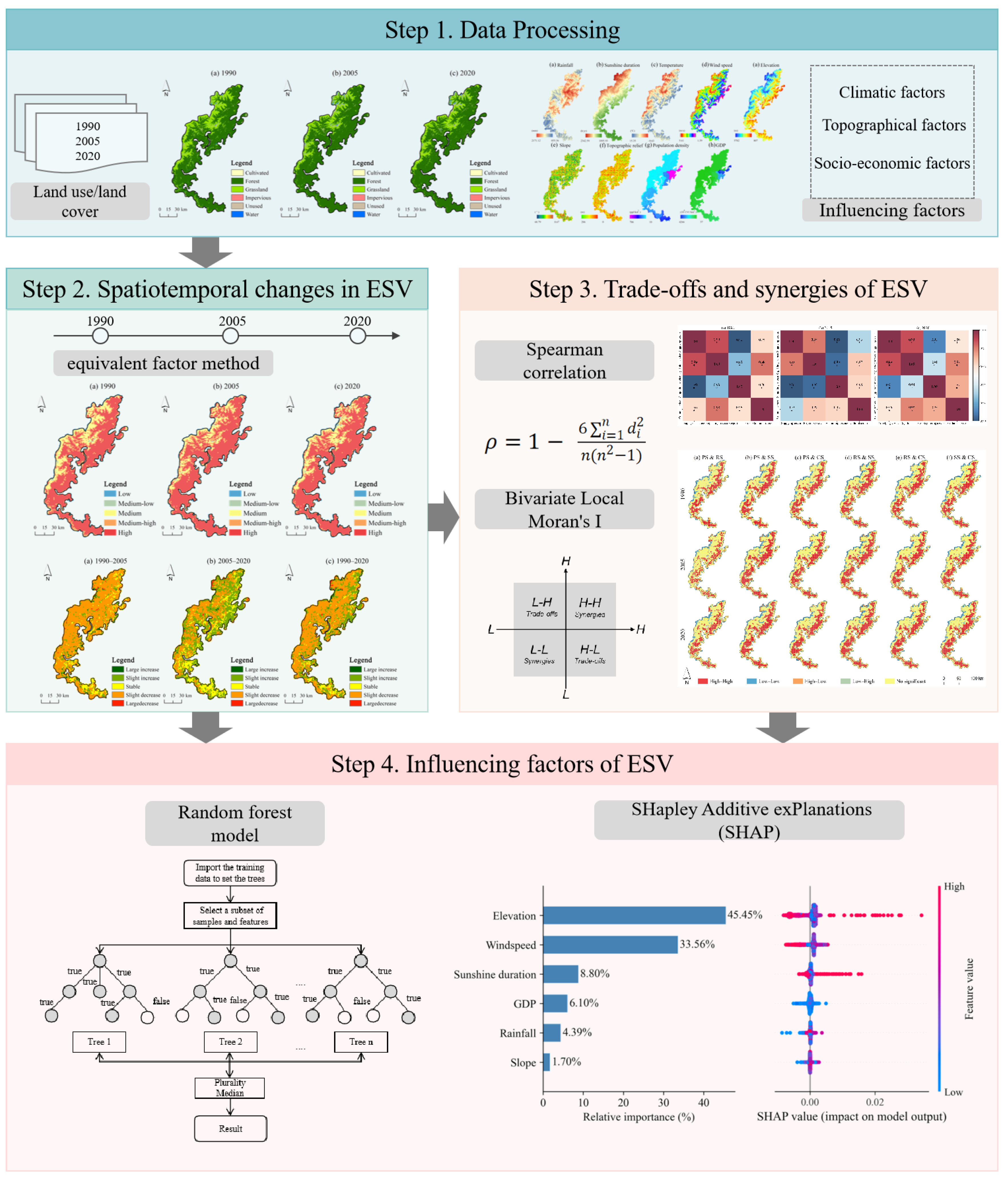
This study aimed to analyze the spatiotemporal evolution, trade-off and synergy relationships, and influencing factors of ESV in the GPNP. First, the ESVs were calculated using the equivalent factor method, and their variation characteristics were analyzed for three evaluation years (1990, 2005, 2020), two intervals (1990–2005, 2005–2020), as well as the overall study period (1990–2020). Second, spatial relationships were explored through linear correlation analysis and bivariate Local Moran’s I analysis to identify trade-offs and synergistic effects. Finally, the RF model and SHAP analysis were employed to identify influencing factors, and based on these analyses, relevant management strategies and recommendations were proposed. The flowchart is shown in Figure 2.

2.2.1. Coefficient Adjustment and Calculation of ESV

In this study, we utilized the equivalent factor method to calculate ESV, adapting the approach based on the land use characteristics of the study area and the findings of previous researchers [46,47]. Based on the ESV equivalent factor correction rules proposed by Xie et al. [48], one standard equivalent factor is defined as one-seventh of the per-area market value of grain (excluding human labor inputs). Then, the dimensionless coefficients were adjusted for each ESV under different land-use types to reflect regional conditions; these coefficients were listed in Appendix A Table A1. The derivation of the unit equivalent value used in monetization is documented in Appendix A Table A2 and Table A3.
To tailor the calculation to the Qionglai–Daxiangling region, we compute the per-area market value of grain as an area-weighted sum over four staple crops (rice, wheat, corn, and beans). The formula used for this calculation is presented as Equation (1).
P = 1 7 k i { r i c e ,   w h e a t ,   c o r n ,   b e a n s } ( s i y i q i )
where s i is Sichuan’s sown-area share of crop (dimensionless), y i is Sichuan’s yield of crop (kg/ha), and q i is the farm-gate price (Chinese yuan (CNY)/kg). The correction factor k captures regional productivity differences and is defined as the ratio of Sichuan’s area-weighted mean grain yield to the national area-weighted mean over the same set of crops and years:
k = i s i y i i s i n a t i o n a l y i n a t i o n a l
The benchmark years 1990, 2005, and 2020 were used (consistent with the study period). Sown areas and yields for Sichuan and China were compiled from the Sichuan Statistical Yearbook and the China Statistical Yearbook; prices were taken from the National Compilation of Costs and Returns of Agricultural Products (see Appendix A Table A2 for inputs). Using Equations (1) and (2), we calculated the unit equivalent value for each of the three benchmark years (1990, 2005, 2020). To mitigate inter-year price volatility, we adopted the geometric mean of these annual values, giving approximately 1057.74 CNY/ha/yr (Appendix A Table A3).
Further calculations were made to determine the mean coefficient of ESV per unit area, which are detailed in Table 1. Following the previous studies [46,47,48], the cultivated water supply service value was assigned a negative coefficient because cultivated evapotranspiration and irrigation demands generally exceed the capacity for water retention, leading to a net depletion of water resources (see Appendix A Table A1). Regarding the basic scale of the study units, researchers experimented with grid scales of 1 km, 1.5 km, 2 km, 2.5 km, and 3 km. After repeated comparisons, a grid size of 1.5 km × 1.5 km was selected because it provides a balance between computational efficiency and the accuracy of spatial heterogeneity representation, particularly for cultivated land and forest patches in the QDR of the GPNP. Ultimately, the study area was divided into 4947 grids. Using the following Equation (3), the ESV for each grid was calculated:
ESV = i = 1 m j = 1 n A j E i j
where A j denotes the area of the j type of land use within each grid, and E i j is the per unit area ESV equivalent for the i ecosystem service function of the j type of ecosystem, which has been adjusted (Table 1). Impervious areas were assigned zero ESV across all services.

2.2.2. Trade-Off and Synergy Analysis of ESV

(1)
Linear Correlation Analysis
In this study, we explored the interactions between different ecosystem services (provisioning services, regulating services, supporting services, and cultural services) in the Giant Panda National Park through linear correlation analysis. We utilized the Spearman correlation analysis method, a non-parametric approach that does not require the data to be normally distributed, suitable for assessing the correlation between two ranked variables [49]. The correlation coefficient ranges from −1 to +1, with values closer to ±1 indicating stronger correlations between the variables. The final results are displayed in the form of a heatmap. The formula was as follows:
ρ = 1   6 i = 1 n d i 2 n ( n 2 1 )
where i = 1 n d i 2 is the sum of the squares of the rank differences between the paired observations. This formula provides a measure of the strength and direction of the monotonic relationship between two ranked variables. d i represents the difference in ranks between the two variables, and n is the number of observations. Additionally, by calculating the p value for each pair of variables, we can assess the statistical significance of the correlations.
(2)
Bivariate Local Moran’s I (Bivariate LISA)
The Local Indicators of Spatial Association (LISA) method was applied to explore the spatial patterns of trade-offs and synergies between different ESVs. This approach not only considers the value of one variable at a specific location but also includes the values of another variable at adjacent locations, thus enabling the exploration of the interactions between two variables [46,50,51]. LISA maps visualize these interactions by mapping the values of local Moran’s I to spatial units. For example, in LISA maps, a high–high (H–H) cluster, where a location and its neighbors both have above-average values, or a low–low (L–L) cluster, where both have below-average values, may indicate a synergy effect. Conversely, high–low (H–L) or low–high (L–H) clusters, where a location and its neighbors have opposite deviations from the average, may suggest a trade-off relationship. The formulas were as follows:
I i ( x , y ) = z i ( x ) j = 1 n w i j z j ( y )
z i ( x ) = x i x ¯ s x ,   z i ( y ) = y i y ¯ s y
s x = i = 1 n ( x i x ¯ ) 2 n 1 ,   s y = i = 1 n ( y i y ¯ ) 2 n 1
where I i ( x , y ) is the bivariate Local Moran’s I for location i in the study area. x i and y j represent the values of two different ESVs for unit i   and its neighbors unit j , respectively. x ¯ and y ¯ are the corresponding means. s x and s y are the standardized deviations, and z i ( x ) and z i ( y ) are the standardized values.   w i j is the element of the spatial weight matrix, defined as First-order Queen Contiguity (FQC) with row standardization, and n is the total number of units. Statistical significance was assessed using 999 random permutations, and the Benjamini–Hochberg false discovery rate (FDR) correction (threshold set at 0.05) was applied to adjust for multiple comparisons. All analyses were conducted in GeoDa (version 1.6.7).

2.2.3. Factors Influencing ESV in the Study Area

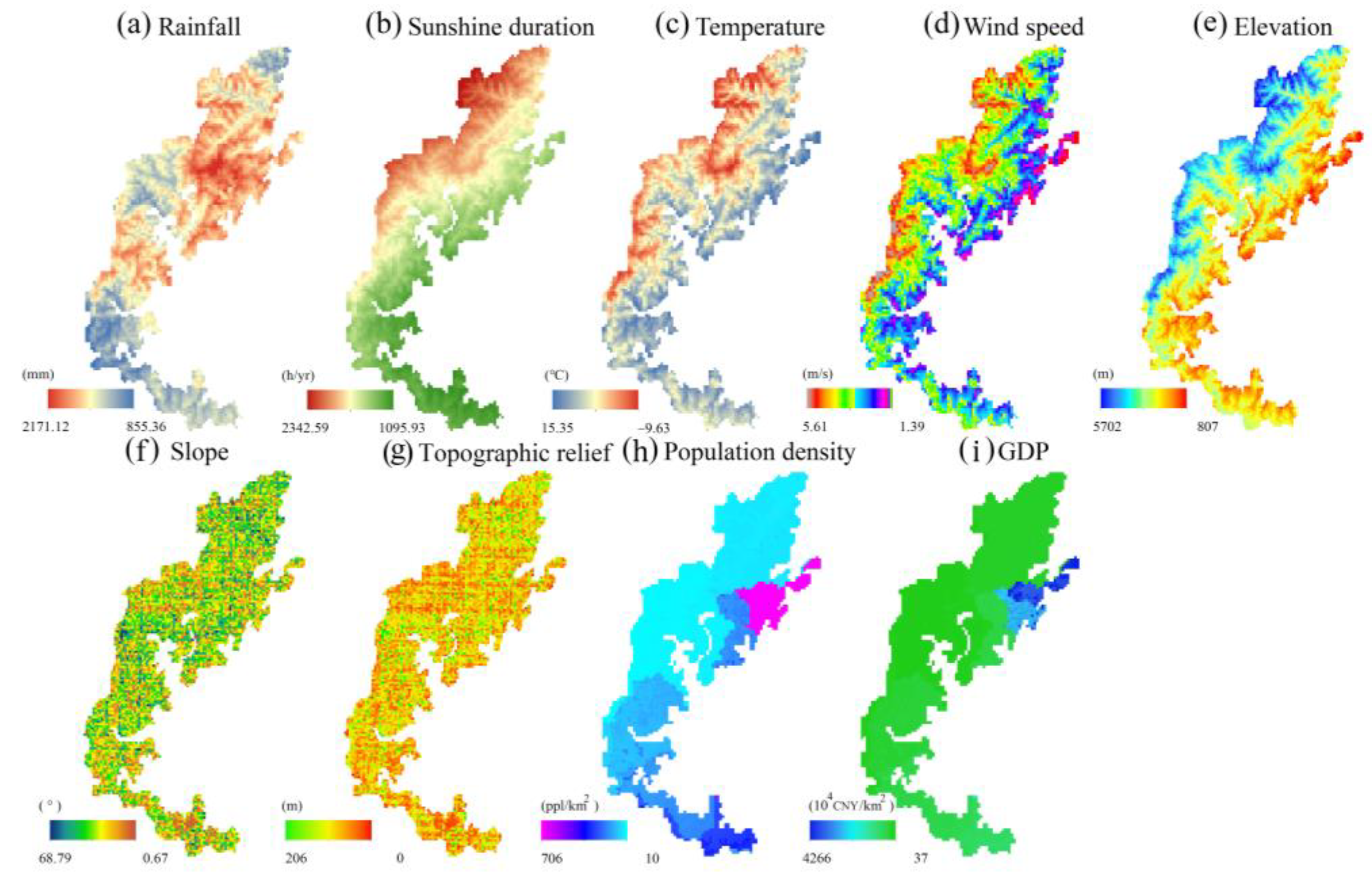
ESV was primarily influenced by natural and socioeconomic factors. Drawing on research from scholars [49], we selected nine influencing factors that cover aspects of climate, topography, and socioeconomics (Table 2, Appendix A Figure A1). These factors were integral to understanding the multifaceted impacts on ESVs and include the following:
(1)
Climatic factors
Rainfall: Influences water availability for various ecosystem services such as water supply and habitat moisture levels.
Sunshine duration: Plays a crucial role in photosynthesis and energy budgets within ecosystems. Longer sunshine duration can enhance plant growth and biodiversity by providing more energy for photosynthetic processes, but it can also increase evapotranspiration rates and potentially stress water resources in arid environments.
Temperature: Affects plant growth, water evaporation rates, and overall climatic conditions within the ecosystem.
Wind speed: Impacts pollination processes, seed dispersal, and microclimatic conditions.
(2)
Topographical factors
Elevation: Determines the type of vegetation and wildlife present, influences microclimates, and impacts the flow of surface and groundwater.
Slope: Affects soil erosion rates, runoff patterns, and the suitability of land for various uses.
Topographic relief: Influences solar radiation receipt, which can affect local temperatures and moisture conditions.
(3)
Socioeconomic factors
Population density: Indicates human pressure on the ecosystem, which can lead to habitat fragmentation and increased pollution.
Gross Domestic Product (GDP): Serves as an indicator of economic activities that can exert pressure on or contribute to the conservation of ESVs.
These factors were meticulously chosen to provide a comprehensive analysis of how both natural phenomena and human activities shape the dynamics of ESVs.
We utilized the RF model to assess the relative importance of all influencing factors [52,53] and then applied SHapley Additive exPlanations (SHAP) values to provide interpretability for the effects of these factors [54]. The SHAP framework, originally proposed by Lundberg and Lee [55], has been increasingly applied in environmental studies—for instance, in assessing hydrological drivers of water quality [56], identifying land degradation risks [57], unveiling environmental drivers of wind erosion [58,59], predicting spatial patterns of geological disasters [60,61], and the effects of the built environment of human activity [62]—demonstrating its effectiveness in enhancing model interpretability within complex socioecological systems. Hyperparameters were tuned via grid search under random K-fold cross-validation, while generalization performance was estimated using spatial K-means block cross-validation. To diagnose residual spatial dependence, we applied Moran’s I with 999 random permutations for global inference and employed BH-FDR correction (q = 0.05) to identify local significance.
For model evaluation, the model’s predictive capability was assessed using Root Mean Square Error (RMSE), the coefficient of determination (R2), and the Mean Absolute Percentage Error (MAPE), calculated as follows:
R M S E = 1 n i = 1 n ( y t r u e , i y p r e d , i ) 2
R 2 = 1 i = 1 n ( y t r u e , i y p r e d , i ) 2 i = 1 n ( y t r u e , i y ¯ t r u e ) 2
M A P E = 100 n i = 1 n | y t u r e , i y p r e d , i y t r u e , i |
where y t r u e , i is the observed value, y p r e d , i is the predicted value, y ¯ t r u e is the mean of the observed data, and n is the number of observations. This approach ensures a comprehensive assessment of how well the model performs in predicting ESV changes based on the selected factors, helping to guide future management decisions and policy formulations effectively.

2.3. Data Source and Processing

The datasets used in this study include multi-year LULC for ESV calculation and trend analysis and climatic, topographic, and socioeconomic data for driver analysis. Specifically, LULC was analyzed for three evaluation years (1990, 2005, 2020) and two intervals (1990–2005, 2005–2020). Climatic and socioeconomic variables were harmonized to 2020 only to focus on the most recent spatial distribution of ESV drivers. In addition, a time series of agricultural statistics (1990–2020) was used exclusively to adjust the ESV equivalence coefficients.
Land use data: Land use data for the years 1990, 2005, and 2020 were selected from the Resource and Data Science Platform (doi: 10.12078/2018070201) at a resolution of 1 km and were classified into six categories: cultivated, forest, grassland, impervious, water, and unused land based on the features in the study area.
Topographic data, including elevation, slope, and topographic relief, were derived from a 30 m Digital Elevation Model (DEM) obtained from the Geospatial Data Cloud (https://www.gscloud.cn/) accessed on 25 August 2025. Topographic relief was calculated as the range of elevation values within each analysis grid cell.
Climatic data: Climatic variables, including precipitation, sunshine duration, temperature, and wind speed, were sourced from the China Meteorological Annual Spatial Interpolation Dataset (doi: 10.12078/2017121301; 1 km resolution). This dataset is produced using the ANUSPLIN thin-plate smoothing spline method with elevation as a covariate, based on annual observations from over 2400 meteorological stations nationwide.
Socioeconomic data: Two types of socioeconomic data were used for different purposes: (a) For ESV equivalence-coefficient adjustment (1990–2020): agricultural statistics (sown area; grain yield per unit area for rice, wheat, corn, and beans; and average grain prices) were gathered from the Sichuan Statistical Yearbook, the Compilation of National Agricultural Product Costs and Returns, and the China Agricultural Product Price Survey Yearbook. These statistics were used to adjust the ESV equivalence coefficients. (b) For driver analysis: population density and GDP raster datasets at a 1 km resolution were obtained from the China Population Spatial Distribution Dataset (doi: 10.12078/2017121101) and the China GDP Spatial Distribution Dataset (doi: 10.12078/2017121102), respectively. Both datasets are generated by spatializing county-level statistics using land-use types, night-time light intensity, and settlement density via a multi-factor weighting approach.
All datasets were projected to the Albers Conic Equal Area coordinate system (units: m) and mapped to the 1.5 km × 1.5 km analysis grid. For LULC data, the nearest-neighbor method was used to aggregate values to the analysis grid, preserving categorical integrity. For partial pixels at the boundaries of the study area, the majority land-cover class within each grid cell was retained without proportional area weighting, consistent with the discrete nature of LULC data. For continuous variables (e.g., climatic variables and DEM-derived metrics), raster layers provided by the data sources were directly clipped to the study area and reprojected to match the analysis grid. No additional interpolation method replacement or topographic adjustment was applied. Missing or anomalous records were handled according to the quality-control procedures of the data providers, and no further gap filling was conducted. Climatic and socioeconomic variables were harmonized to the year 2020 to focus on the most recent spatial distribution of ESV drivers, to avoid redundancy from multi-year driver analyses, and because the relative importance ranking of drivers is assumed to remain relatively stable over the study period.

3. Results

3.1. Spatiotemporal Variation in Land Use and ESV

3.1.1. Changes in Land-Use/Land-Cover (LULC)

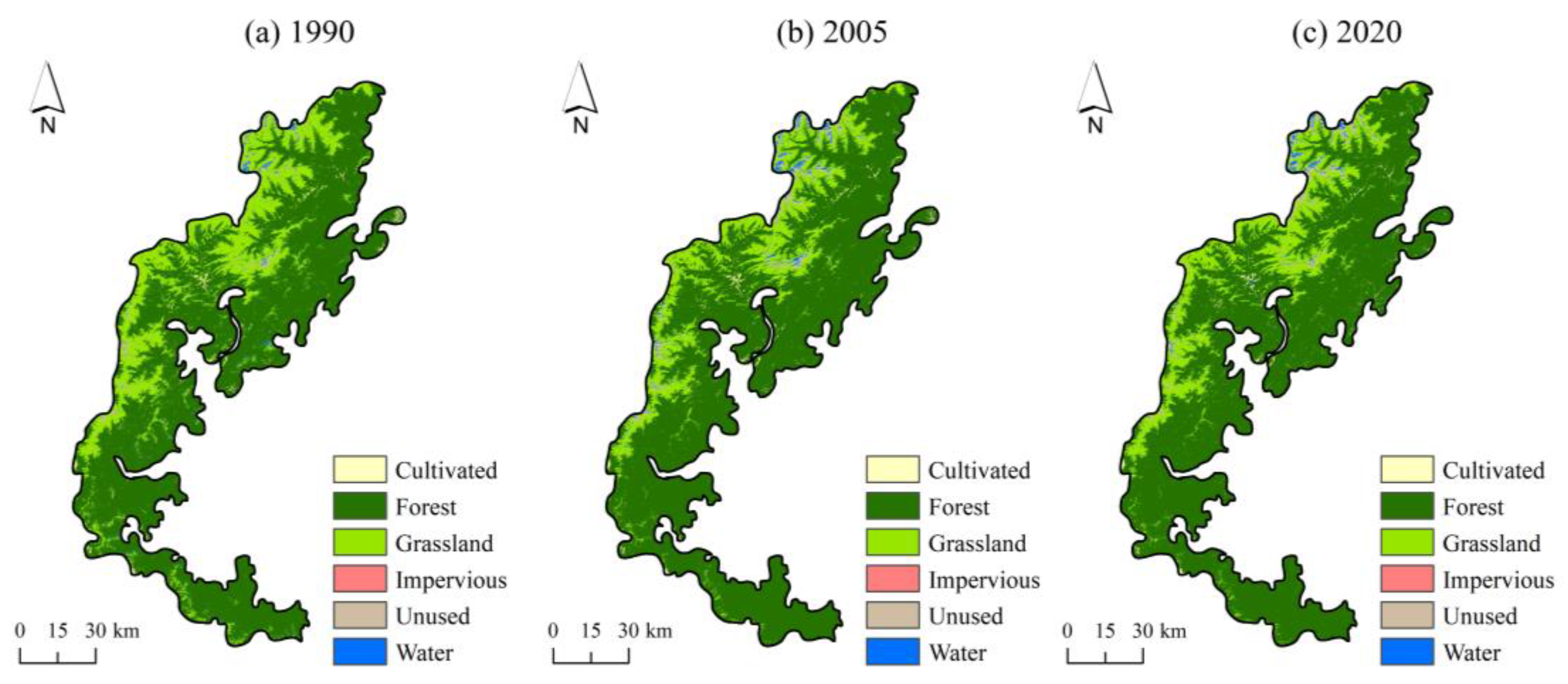
Table 3 indicated that forest and grassland were the predominant land use types in the study area, together accounting for over 95% of the total area, thereby providing significant support for ecosystem services. According to the 2020 land use statistics, forested areas constitute 78.21% of the study area, followed by grasslands at 18.31%. Over time, from 1990 to 2020, forested areas exhibited a steady increase, growing by 407.62 km2, representing a growth of 5.46%. In contrast, grassland areas decreased by 479.69 km2, a reduction of 20.66%. Similar to cultivated areas, the areas of water and unused land displayed fluctuating trends but generally increased. Notably, the area of impervious surfaces continuously expanded; although it only increased by 1.17 km2 over the past 30 years, the increase amounted to 205.26%, reflecting significant urban development in the study area. Regarding temporal changes, the cultivated area overall showed fluctuating trends: from 1990 to 2005, a significant decrease of 14.65 km2, whereas from 2005 to 2020, a notable increase of 13.82 km2, reflecting the significant impact of national policies such as RFFP and cultivated protection on land use changes. Spatial distribution analysis (Figure 3) reveals that forested areas cover the vast majority of the study region; grasslands were concentrated on the northwestern side, while cultivated, water, unused land, and impervious areas were dispersed throughout the area. Such a land use pattern exhibited significant spatial heterogeneity, reflecting a substantial influence from the topographic features of the landscape.

3.1.2. Changes in ESV

Table 4 shows the changes in ESV from 1990 to 2020 in the QDR of the GPNP. The overall change in ESV during this period was minimal, displaying an inverted V-shape, with the peak value reaching CNY 195.11 billion in 2005. In 1990 and 2020, the ESVs were CNY 190.61 billion and CNY 193.23 billion, respectively. Regarding the contributions by land use type, forests and grasslands contributed the highest to the ESV, followed by water, cultivated, and unused lands. For instance, in 2020, the ESV of forested areas was CNY 163.53 billion, accounting for 84.63% of the total ESV, followed by grasslands, with a value of CNY 23.51 billion, which constituted 12.17% of the total. This highlighted the unique significance of forests and grasslands in the ESV of the QDR, underscoring their critical role in this region.
Figure 4 and Figure 5 illustrate the spatial patterns and evolution of ESVs over the past three decades. To enhance comparability, we adopted the Jenks natural breaks method to classify both the absolute values of ESVs and their changes into five categories. Specifically, ESV levels were divided into Low, Medium-low, Medium, Medium-high, and High (Figure 4), while ESV changes were categorized as Large decrease, Slight decrease, Stable, Slight increase, and Large increase (Figure 5). The natural breaks method was selected because it minimizes intra-class variance while maximizing inter-class variance, thereby ensuring that the classification boundaries are determined objectively by the data distribution itself. Compared with equal-interval or quantile methods, the natural breaks approach better captures the inherent heterogeneity of ESV data across complex mountain landscapes, making it more suitable for revealing spatial gradients and identifying areas with significant ecological change. Spatially, the high-value segments of ecosystem services occupied the majority of the study area. Over time, the spatial pattern significantly altered. In terms of the evolution of ESV from 1990 to 2020, despite overall fluctuations, the majority of the area experienced a Slight decrease in ESVs; however, from 2005 to 2020, most of the area showed a Slight increase in ESVs. These findings suggested that while there were periods of decline in ESVs across the study area, recent trends indicate a recovery, possibly reflecting effective conservation measures or changes in environmental management strategies. Such patterns highlight the dynamic nature of ESVs and underscore the importance of continuous monitoring and adaptive management to sustain and enhance these vital services.

3.2. Trade-Offs and Synergies Among ESVs

Figure 6 displays the correlations among four types of ecosystem services (provisioning, regulating, supporting, and cultural services) within the GPNP for the years 1990, 2005, and 2020. We computed pairwise Spearman correlations among service categories for each evaluation year and adjusted p-values using the Bonferroni correction within each year (α = 0.05). The diagram revealed that, at these three time points, most services exhibited strong positive correlations, particularly between provisioning and supporting services, which consistently show very high correlations (above 0.90). This indicated that as provisioning services (such as water and food supply) were enhanced, supporting services (such as soil formation and nutrient cycling) were also strengthened, reflecting the natural interconnections within ecological processes. The correlation between regulating services and other services was also high, illustrating the supportive role of regulating services (such as climate regulation and disease control) regarding other ecosystem services. The enhancement of such services further benefited other services, including provisioning and cultural services, which may encompass educational and recreational activities.
Notably, the correlation between provisioning and cultural services decreased from 1990 to 2020. This decline was likely due to changes over time in the way natural resources were utilized, driven by regional ecological protection policies and socioeconomic development, such as increased focus on the sustainable use of ecosystems and the enhancement of their cultural values.
Overall, these strong correlations indicate that the synergistic interactions among provisioning, regulating, supporting, and cultural services have strengthened over time. This enhancement was likely linked to the Chinese government’s efforts in ecological protection and sustainable management. As policies such as RFFP were implemented, natural habitats were restored and the multifunctionality of ecosystems was enhanced. This not only increased the value of individual services but also strengthened the mutual support among various services. Such enhanced synergy aids in achieving the overarching goals of ecosystem management, namely, improving ecosystem functionality and its capacity to withstand external pressures.
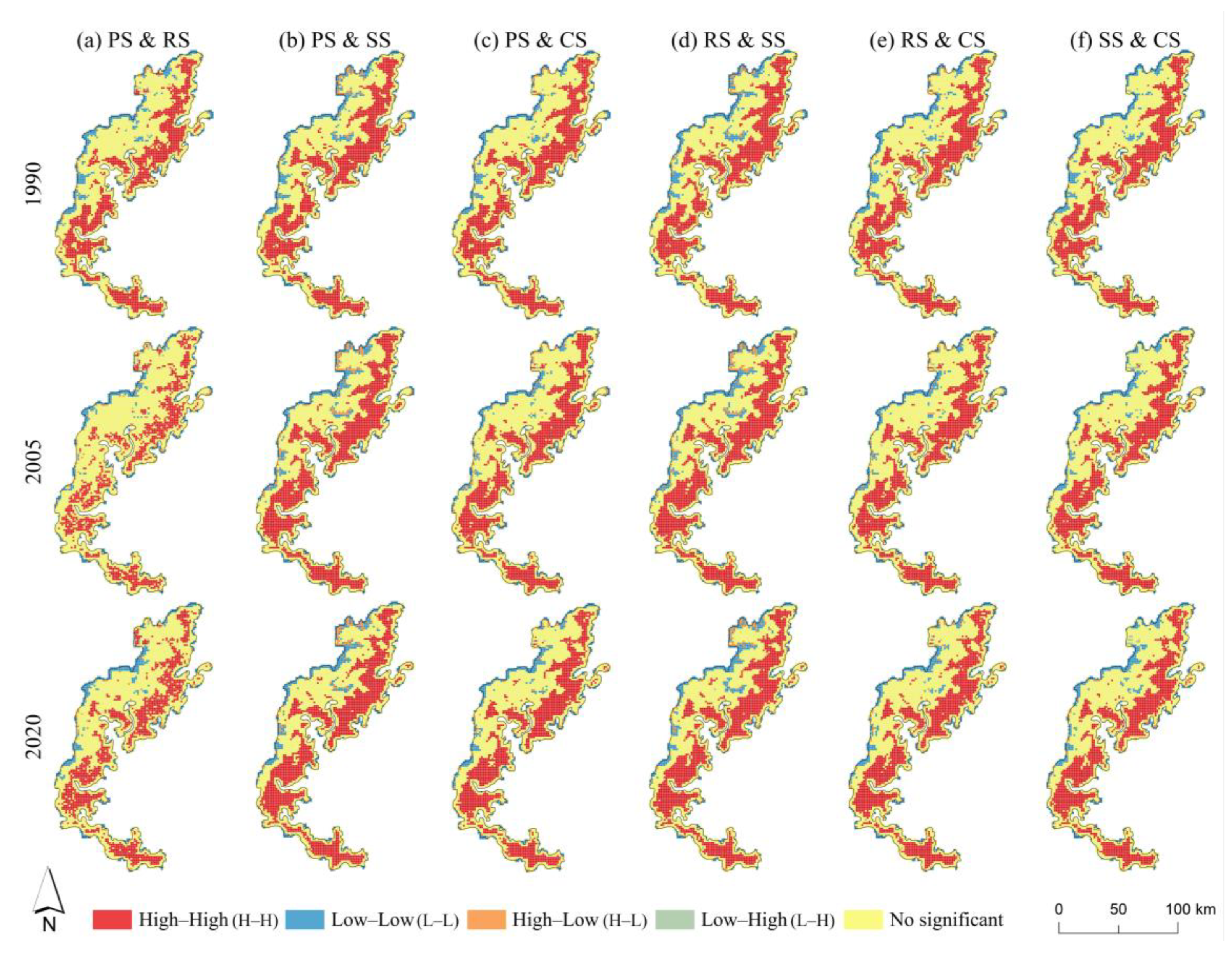
Figure 7 presents the results of the Local Moran’s I analysis, which examined the interactions between different ESVs in the GPNP for 1990, 2005, and 2020. The “H–H” (red) areas indicated that both services are above average, showing enhanced synergy; the “L–L” (blue) areas indicated that both services are below average, which suggested a deficiency in these services or a reduction in their synergy. “High–High” (H–H, red) clusters indicate areas where both services are above average, reflecting strong synergistic effects; “Low–Low” (L–L, blue) clusters represent areas where both services are below average, suggesting weakened or deficient synergies. “High–Low” (H–L, brown) and “Low–High” (L–H, green) clusters illustrate trade-offs, where one service exhibits higher values while the other remains relatively low. Regions shown in yellow indicate statistically insignificant spatial associations.
From 1990 to 2020, the spatial configuration of these clusters changed considerably. H–H clusters were concentrated in high-altitude mountainous areas characterized by dense vegetation and low human activity, where ecological integrity supported strong synergies. In contrast, L–L clusters were primarily found in low-altitude plains and hilly regions with high population density and intensive land use, where provisioning services often expanded at the expense of regulating services, generating stronger trade-offs. Notably, some areas that displayed significant H–H synergy in 1990 shifted to non-significant patterns by 2020, reflecting the dynamic interplay of ecological processes and policy interventions.
These dynamics are closely linked to both natural factors and ecological restoration programs. For example, the Returning Farmland to Forest Program (RFFP, tuigeng huanlin gongcheng) altered land-use structures by converting cultivated land into forest and grassland, which enhanced vegetation cover, increased carbon sequestration, and improved water regulation. This policy-driven vegetation recovery played a pivotal role in strengthening synergies between provisioning and regulating services. By contrast, areas with persistent L–L clustering were often those where population growth and urban expansion intensified land use pressure, leading to ecological degradation and reduced service synergies. Overall, these results highlight the spatial heterogeneity of trade-offs and synergies, shaped jointly by terrain constraints and anthropogenic drivers.

3.3. Influencing Factors of ESV

To assess and mitigate multicollinearity, we computed the pairwise Pearson correlations and Variance Inflation Factor (VIF) for all predictors. Variables with a VIF > 10 were iteratively removed until all remaining predictors had a VIF < 10. The final predictor set consisted of GDP (1.38), Sunshine duration (2.90), Rainfall (1.47), Slope (1.02), Elevation (9.83), and Wind speed (6.94). Then, a correlation matrix of the selected predictors was presented (Figure 8). The optimal parameters of the RF model were determined through grid search with random fivefold cross-validation (CV) (‘max_depth’: 9, ‘max_features’: 3, ‘n_estimators’: 60), after which model performance was evaluated under three schemes: random K-fold, spatial Grid, and spatial K-means partitions, respectively (Table 5).
To avoid the potential overestimation of predictive performance caused by random partitioning in spatial data, the K-means spatial block cross-validation was adopted as the final evaluation scheme. Finally, the RF model was refitted on the full dataset for SHAP interpretation, and the results were illustrated with a relative importance bar plot and a beeswarm plot. Finally, under the final K-means spatial CV, out-of-fold residuals exhibited a Moran’s I of 0.209, p = 0.005, indicating that spatial autocorrelation in residuals was significant (see Appendix A Figure A2). This result suggests that although the spatial K-means partitioning approach reduced autocorrelation compared with random K-fold and spatial Grid partitions, spatial dependence in the residuals remained, implying that additional spatial processes not captured by the predictors may still be influencing the model outcomes. The diagnostic plots in Figure A2 further illustrate the global significance and the lack of localized clusters after BH-FDR correction.
Figure 9 presents the relative importance of the selected predictors (left) and a beeswarm plot illustrating their marginal contributions (right). From the bar chart, elevation (45.45%) and wind speed (33.56%) emerged as the dominant drivers of ESV variation, jointly accounting for nearly 80% of the total importance. Elevation exerted the strongest effect: higher elevation values generally increased predicted ESV, suggesting that less human disturbance and better ecological preservation in mountainous areas may favor ecosystem service provision. Wind speed also showed a strong positive contribution, reflecting the role of regional climatic dynamics in shaping ESV distribution. Other variables, including sunshine duration (8.80%), GDP (6.10%), rainfall (4.39%), and slope (1.70%), contributed modestly to model performance. Their relatively lower importance indicates that while socioeconomic and secondary environmental factors influence ESV, their impact is substantially weaker compared with topographic and climatic determinants. The beeswarm plot provides further insights into the direction and distribution of feature effects. High elevation and high wind speed values are consistently associated with positive SHAP contributions, while low values of these predictors drive negative contributions. Sunshine duration also tends to have a positive effect, although with a smaller magnitude. Interestingly, GDP, rainfall, and slope exhibit both positive and negative SHAP values, suggesting context-dependent influences in different locations. Together, these results highlight that topography (elevation) and climate (wind speed and sunshine duration) are the primary determinants of ESV patterns in 2020, whereas socioeconomic drivers play only a secondary role. This underscores the critical importance of natural geographic constraints in shaping ecosystem service capacity.
Additionally, climatic factors had a significant impact on ESV. This finding aligned with research by Yang et al. [63] conducted in the source region of the Yellow River, underscoring the need for greater scholarly attention to how climate change poses a potential yet often overlooked challenge to the protection and management of ecosystem services.

4. Discussion

4.1. The Importance of ESV in National Parks

National parks, as key regions for maintaining national ecological security, play a crucial role in global ecological conservation and biodiversity preservation [6,22]. Especially in the face of ecological degradation and climate change, the ESV in national parks is significantly important for the protection of biodiversity and for socioeconomic benefits [22,27]. Establishing protected areas provides many species with relatively undisturbed habitats, which is particularly vital for species that require large living spaces or are especially sensitive to environmental changes. The biodiversity within national parks also helps maintain ecosystem functionality, playing an irreplaceable role in resisting and adapting to environmental changes. Moreover, national parks play an indispensable role in maintaining water quality, air quality, and soil health. The GPNP, as an important conservation area for biodiversity in Southwest China, carries the critical mission of protecting the endangered giant panda and its ecological environment. The survival of the giant panda depends on continuous and stable bamboo forest habitats. However, these habitats often face the threat of fragmentation due to natural environmental changes and human activities. In this context, constructing ecological networks, especially ecological corridors, becomes an effective way to connect isolated habitats and ensure the free migration of giant pandas and other species. These findings underscore that ecological corridors should be prioritized in future management planning for the GPNP.
While these ecological insights highlight the importance of enhancing connectivity and sustaining ESVs in the GPNP, it is equally important to position our findings within the broader research context. Previous studies on the GPNP have provided valuable insights but differ in scope and methodological emphasis. For instance, previous research on ecological sensitivity employed an indicator-based system, which provided spatial insights but did not capture the long-term ESV dynamics of the GPNP [20]. Similarly, another study examined the relationship between giant panda populations and ecosystem services [44], but their analysis was primarily correlation-based and confined to relatively short timeframes. In contrast, this study introduces a distinctive methodological integration of the modified equivalent factor method with an RF model and SHAP analysis, which enables both the quantification of ESV and the interpretation of nonlinear drivers. Moreover, by investigating the 30-year dynamics from 1990 to 2020, our research adds temporal depth that has been largely absent from previous work, thereby providing a novel contribution to understanding ecosystem service changes in the GPNP.

4.2. Changes in ESV and Their Responses to Land Use Changes

Land use change is a major factor affecting ESV, directly altering the structure and function of ecosystems, with different types of land use contributing and impacting ecosystem services in varied ways [6,9,22,29,36,63,64]. In this study, we observed significant changes in the land use structure in the QDR from 1990 to 2020, particularly the reduction in cultivated land and grassland and the increase in forested land, reflecting major adjustments in regional ecological protection and land management strategies. By deeply analyzing these changes and their association with ESV, we can better understand the long-term impacts of land management policies on the ecological environment. Over the past thirty years, the significant reduction in cultivated land in the area has been closely linked to the RFFP, implemented in 1999. This important ecological restoration initiative aims to restore forests and grasslands by reducing cultivated land, minimizing soil erosion, and improving the ecological environment [65,66,67]. We found that this policy not only increased forested areas but also facilitated the restoration of biodiversity and the enhancement of ecosystem functions, a conclusion supported by related research [29,68]. However, the implementation of this policy also led to a reduction in grassland area, especially in areas where topographic relief and climatic conditions are suitable for forest growth. The increase in forested land has significantly influenced ESV, bringing both substantial benefits and certain trade-offs. Forest ecosystems, known for their role as crucial carbon storage sites, provide diverse ecological services, including regulating water cycles, maintaining soil stability, and supporting biodiversity. These services have been notably enhanced with the expansion of forested areas, particularly in regions where topographic relief and climatic conditions favor forest growth. However, the replacement of grasslands by forests may alter water retention dynamics and habitat availability, potentially leading to shifts in ecosystem functions. While forests contribute positively to many ecological processes, it is important to recognize that these changes may also reflect a reconfiguration of ecosystem service provisioning rather than a uniform improvement across all dimensions. Additionally, the recreational and aesthetic values of forests have brought new economic opportunities to local communities, especially in terms of ecotourism. Nevertheless, while the increase in forested areas has brought many positive effects, the reduction in grassland has also triggered a series of environmental issues. Grassland ecosystems play a crucial role in maintaining local climate balance, protecting soil from erosion, and supporting specific herbivorous animal populations. Moreover, the reduction in grassland could lead to the partial loss of ecosystem services, potentially affecting functions such as water retention and biodiversity maintenance.
Importantly, this study reveals the specific impacts of land use changes on ESV, and we call for more scholars and policymakers to focus on the significant impacts of land management and ecological restoration on ESV. These results highlight the need for the careful consideration of land-use policies, as both positive and negative ecological outcomes may arise. Specific recommendations for management practice are provided in the Practical Implications section.

4.3. Implications of ESV Trade-Offs and Synergies

In ecosystem management, the relationships among services, trade-offs, synergies, and independencies form a complex network of interactions [69,70]. Trade-offs occur when the enhancement of one service comes at the expense of another; for example, increased agricultural production may lead to a decline in water quality. Synergies, on the other hand, occur when the enhancement of one service also enhances another, such as forest conservation, which supports carbon storage, water retention, and biodiversity protection. Independent relationships imply that changes in one service do not significantly affect others. A deep understanding of these trade-offs and synergies is crucial to ensuring the maximization of overall ecosystem functionality and services, as overlooking these relationships can threaten the functionality and safety of the entire ecosystem [71,72,73]. Moreover, these relationships are affected by spatial scale effects, displaying a high degree of uncertainty. For instance, services may exhibit synergistic relationships at a smaller spatial scale, which might shift to trade-offs at a larger scale, adding complexity and challenges to ecosystem service management [49,74,75].
It is commendable that the Chinese government places high importance on Ecological Civilization Construction (ECC, Shengtai Wenming Jianshe), a framework emphasizing ecological protection, sustainable development, and harmony between socioeconomic systems and the natural environment, significantly improving the overall condition of ecosystems through a series of innovative policies and mechanisms. These policies include the renowned RFFP, wetland protection plans, and ecological compensation mechanisms, which not only directly enhance the quality of specific ecosystem services but also promote synergistic effects among different services. In this study, analyzing data from 1990 to 2020 for the Giant Panda National Park, we observed that the synergistic effects of ecosystem services not only strengthened year by year but also became the dominant trend in the region’s ecological protection achievements. This positive change is underpinned by the Chinese government’s firm commitment to and actions towards ecological civilization. The implementation of the RFFP policy, for example, has successfully transformed a large amount of overcultivated land into forests and grasslands with richer ecological functions, aiding in soil conservation and water retention and enhancing biodiversity protection. Meanwhile, wetland protection measures ensure the purity of water and the integrity of habitats, thus enhancing the ecosystem’s self-recovery capabilities and functionality nationwide. The introduction of ecological compensation mechanisms further motivates local governments and communities to actively participate in ecological conservation. Economic compensation ensures that local communities, which might lose income due to conservation measures, are adequately supported, enhancing their enthusiasm for participating in ecological conservation and helping them understand and support long-term ecological restoration goals. Overall, the implementation of these policies has not only improved the ecological environment of the Giant Panda National Park and its surrounding areas but also provided valuable experiences and examples for global ecological conservation.
This study reveals how different ecosystem services interact within the GPNP and how they change over time and across spatial scales. For instance, the increase in forested areas not only boosts carbon storage but also improves water quality and biodiversity, showing strong synergistic relationships among ecological services. These findings provide a crucial scientific basis for future ESV management, particularly in developing strategies that maximize synergistic benefits and minimize trade-off losses. Given the uncertainty and complexity in the relationships among ecosystem services, future research needs to further explore the dynamic changes in different ecosystem services under various environmental conditions and policy contexts. Additionally, studies should expand to more scales and ecosystem types to fully understand the trade-offs and synergies of ecosystem services, ensuring the effectiveness and adaptability of ecosystem management strategies.

4.4. Interpretation of Influencing Factors of ESV

ESVs are subject to the complex influences of natural environments, socioeconomic factors, and human activities [76]. For instance, climatic conditions such as temperature, precipitation, and wind speed directly affect plant growth, water availability, and the material cycles of ecosystems. Geographic location determines the amount of solar radiation an ecosystem receives and the characteristics of the regional climate, thereby influencing vegetation cover and ecosystem types. These factors interact to shape the patterns of ESV. For example, global warming may increase the value of certain services such as carbon storage by altering vegetation types and distribution while simultaneously reducing the value of other services, such as the glacial water supply. Socioeconomic development can provide resources for ecological protection and restoration, but it may also increase the consumption of natural resources and damage ecosystems [77]. The implementation of policies and management acts as a critical intermediary that can coordinate the impacts of natural and socioeconomic factors, enhancing the maximization of ESV.
Additionally, our findings exhibit consistencies with international evidence while providing context-specific insights. First, similar to studies in Southeast Asia, forests in the QDR were identified as key providers of multiple services, reinforcing the importance of natural land cover types for maintaining ecological integrity and supporting opportunities such as ecotourism [26,27]. Second, evidence from Germany and the United States indicates that recreational and cultural values vary widely across parks, influenced not only by ecological attributes but also by landscape settings and stakeholder engagement [25]. This resonates with our finding that climatic and topographic gradients strongly shape ES provision in mountainous parks. Collectively, these connections indicate that while our study is grounded in the QDR of the GPNP, its workflow and findings are also relevant to broader discussions on ESV assessment in protected landscapes.
In this study, we employed a combination of RF models and SHAP value analysis not only to assess the relative importance of each factor but also to provide interpretability for the specific impact of each factor on ESV. Elevation, wind speed, and sunshine duration emerged as the dominant factors influencing ecosystem services, an insight crucial for understanding how ecosystems respond to changes in the natural environment. This finding is consistent with the research by Zhang et al. [49], which identified climatic conditions as key drivers of growth for agricultural and forestry crops, positively influencing ESV. Notably, we integrated advanced machine learning techniques with classical ESV assessment methods, providing a comprehensive analytical framework for the changes in ESV. Our approach offers new tools and perspectives for future research on ecosystem services and environmental management, capable of revealing more complex causative relationships and dynamic changes. Compared to related studies, our work emphasizes the interpretability of model predictions, a factor often underconsidered in previous ecosystem service research. The application of SHAP values enhanced our analysis, enabling us to precisely identify which factors are most critical to changes in ESV and to quantitatively analyze how these factors interact. However, it is important to note that in such large-scale studies, the effects of influencing factors are subject to scale effects, meaning that the drivers may exhibit spatial heterogeneity [9,78]. This topic will be a forward-looking subject in research on factors affecting ecosystem services in national parks. In addition, uncertainties may arise from the static equivalent factor method and the resolution of input datasets. Therefore, SHAP results should be regarded as relative rather than absolute measures of factor importance. Future research could combine SHAP with spatially explicit statistical approaches, such as Geographically Weighted Regression (GWR), spatial lag/error models, or multi-scale GWR, to better account for spatial non-stationarity and heterogeneity in ESV dynamics [79].

4.5. Limitations and Future Directions

This study selected nine key factors for evaluating the impacts of land use changes on ESVs. We acknowledge that in complex social-ecological systems, a limited number of factors may not fully capture the dynamic characteristics of these systems. However, including too many factors could increase model complexity, leading to potential multicollinearity issues and overfitting. Additionally, incorporating a larger number of factors often requires higher-quality and more extensive data, which may not always be available for our study area in particular. Future studies could refine variable selection processes and incorporate additional relevant factors.
Although this study adopted a traditional ecosystem services classification system (including supporting services), we recognize that this approach may appear outdated in modern ecosystem services research. For example, the CICES framework no longer categorizes supporting services as a standalone group, as they are considered inherent to other services. However, in the context of the GPNP, the traditional classification demonstrates specific advantages. The park is dominated by mountainous ecosystems where biodiversity maintenance, soil conservation, and hydrological regulation are critical to sustaining the habitat of giant pandas and other rare species. These functions are explicitly represented under “supporting services” in the traditional system but are less directly emphasized in CICES. Moreover, the equivalent factor method employed in this study was originally designed to match the traditional classification, which allows us to capture the contribution of biodiversity support, soil stabilization, and nutrient cycling—processes that are fundamental to maintaining ecosystem stability in fragile alpine and forest environments. Future research could consider adopting or integrating the CICES framework to improve international comparability while retaining the advantages of explicitly accounting for supporting services in protected areas.
In addition, the study acknowledges a limitation in not fully addressing the spatial heterogeneity of ecological compensation policies. In the GPNP, the intensity of the RFFP has varied significantly between regions. For example, subsidies were typically higher in the steep mountain valleys of western Sichuan, where cultivated conversion was ecologically urgent, compared to the relatively low-intensity implementation in the eastern foothills and plains. This uneven distribution of compensation intensity is likely to have contributed to the differentiated patterns of ESV change observed in our results. However, the present study did not explicitly incorporate quantitative measures of subsidy allocation into the analysis. Future work should integrate ecological compensation variables, such as regional subsidy intensity and coverage, to better reveal how policy interventions shape spatially heterogeneous ESV dynamics within national parks.
Beyond methodological considerations, the results of this study provide several practical insights for the management of the GPNP and other protected mountainous regions. First, high-value and high-synergy clusters should be prioritized for strict protection and ecological connectivity maintenance, as these areas simultaneously deliver multiple services and support biodiversity conservation. Second, low-value and low-synergy zones represent potential targets for ecological restoration, such as vegetation enhancement and soil improvement, depending on local feasibility. Third, given the strong associations between ESV and climatic/topographic factors such as temperature and elevation, managers should strengthen monitoring in climate-sensitive areas to anticipate possible service fluctuations under environmental change. Fourth, regularly updating land-use data is essential to detecting newly emerging trade-off hotspots, ensuring timely adjustments in conservation and zoning strategies. Finally, the integrated workflow of multi-temporal ESV assessment, trade-off/synergy mapping, and interpretable driver analysis is readily transferable to other protected areas by adapting equivalence factors and incorporating region-specific drivers. These implications complement the findings discussed in Section 4.1, Section 4.2 and Section 4.3, offering more actionable recommendations for management practice.

5. Conclusions

This study provides a comprehensive understanding of ESVs and their driving factors, offering valuable guidance for the management and conservation of national parks. By integrating the revised equivalent factor table method, RF models, and SHAP value analysis, the research presents a detailed exploration of changes in ESVs and their underlying mechanisms in the QDR of the GPNP. The results show that elevation, wind speed, and sunshine duration are most strongly associated with ESV variation, reflecting the dominant roles of topographic and climatic controls in mountainous environments. Moreover, the study identifies increasing synergies among ecosystem services over the past three decades, suggesting land-use policies, such as the RFFP, contributed to these trends.
Overall, this study underscores the importance of understanding the interactions between natural and anthropogenic factors in shaping ESVs, particularly in ecologically sensitive and biodiversity-rich regions. The insights gained provide a foundation for the sustainable management of national parks and offer valuable lessons for global conservation efforts amid the challenges of climate change and human activities. In addition to theoretical contributions, this study also provides practical recommendations: managers should prioritize high-synergy clusters for protection, target low-value zones for ecological restoration, strengthen monitoring in climate-sensitive areas, and regularly update land-use information to detect emerging trade-offs. These recommendations highlight the transferability of the proposed workflow and its value as a decision support tool for other protected mountainous regions worldwide.

Author Contributions

Conceptualization, Y.C. and M.A.-B.; methodology, Y.C. and R.Z.; software, Y.C. and L.D.; validation, Y.C., L.D. and M.A.-B.; formal analysis, Y.C. and R.Z.; investigation, Y.C., R.Z. and M.A.-B.; data curation, Y.C.; writing—original draft preparation, Y.C., R.Z. and M.A.-B.; writing—review and editing, Y.C. and M.A.-B.; visualization, Y.C. and L.D.; supervision, M.A.-B.; funding acquisition, Y.C. and M.A.-B. All authors have read and agreed to the published version of the manuscript.

Funding

This research was supported by the National Natural Science Foundation of China (Grant No. 52308081), the Philosophy and Social Science Foundation in Chengdu City (Grant No. 2024BS059), the Key Research Institution of Philosophy and Social Science in Sichuan Province: Research Center for Rural Development in Sichuan province (Grant No. CR2411), and the Fundamental Research Funds for the Central Universities (Grant No. 2682024CX126).

Data Availability Statement

The data presented in this study are available from the corresponding author upon request.

Conflicts of Interest

The authors declare no conflict of interest.

Abbreviations

CICESCommon International Classification of Ecosystem Services
CVcross-validation
DEMdigital elevation model
ESVecosystem service value
GDPgross domestic product
GPNPGiant Panda National Park
LISALocal Indicators of Spatial Association
LULCland use/land cover
MAPEmean absolute percentage error
MEAMillennium Ecosystem Assessment
PAMphysical assessment method
QDRQionglai–Daxiangling region
RFFPReturning Farmland to Forest Program
RMSEroot mean square error
SHAPShapley Additive exPlanations
VAMvalue assessment method
VIFvariance inflation factor

Appendix A

Figure A1. Spatial distribution of the nine influencing factors affecting ESV.
Systems 13 00807 g0a1
Table A1. Adjusted equivalent factor coefficients of ecosystem services for different land-use types (dimensionless).
Primary ServicesSecondary ServicesCultivatedForestGrasslandWaterUnused
Provisioning ServicesFood production1.000.250.230.440.00
Raw material production0.310.580.340.240.00
Water supply−0.780.300.194.350.00
Regulating ServicesGas regulation0.801.911.210.950.02
Climate regulation0.425.713.192.140.00
Purifying the environment0.121.671.053.100.10
Hydrological regulation1.013.742.3444.530.03
Supporting ServicesSoil conservation0.722.321.471.080.02
Maintaining nutrient circulation0.140.180.110.080.00
Biodiversity0.152.121.343.480.02
Cultural
Services
Aesthetic landscape0.070.930.592.240.01
Table A2. Input data for computing the unit equivalent value P (benchmark years 1990, 2005, 2020).
YearStatistical ScopeRiceWheatCornBeans
Sown Area
(ha)
Grain Yield
(kg/ha)
Price
(CNY/kg)
Sown Area
(ha)
Grain Yield
(kg/ha)
Price
(CNY/kg)
Sown Area
(ha)
Grain Yield
(kg/ha)
Price
(CNY/kg)
Sown Area
(ha)
Grain Yield
(kg/ha)
Price
(CNY/kg)
1990Sichuan Province 2,300,0007394.78 1,680,0003398.21 1,199,0004054.21 343,0001848.40
China (national)33,064,0006211.950.5830,753,0003454.950.6121,401,0005374.280.449,163,0001506.221.17
2005Sichuan Province 1,995,0007655.22 1,360,0003993.53 1,185,0005414.58 520,0002364.51
China (national)28,847,00064651.5522,793,00048871.3826,358,00063391.1112,901,00019832.57
2020Sichuan Province 18660007904.95 597,0004134.37 1,839,0005790.02 599,0002316.08
China (national)30,076,0007016.852.7523,380,0006454.952.2841,264,0007539.32.3111,593,0002003.44.86
Note: Scope denotes the statistical scope of the data source: “Sichuan Province” refers to provincial-level statistics; “China (national)” refers to national averages. Units: sown area (ha), yield (kg/ha), price (CNY/kg). Data sources: Sichuan Statistical Yearbook; China Statistical Yearbook; National Compilation of Costs and Returns of Agricultural Products. National average prices were uniformly used for the calculation.
Table A3. Derived correction factor k and unit equivalent value P (benchmark years 1990, 2005, 2020).
Yeark (−)P (CNY/ha/yr)
19901.10459.60
20051.041214.87
20200.912059.65
Geometric mean 1057.74
Figure A2. Spatial diagnostic plots of model residuals under the final spatial cross-validation. In the Moran’s I scatterplot, the points represent the standardized residuals, and the line indicates the fitted spatial trend.
Systems 13 00807 g0a2

References

  1. Lahon, D.; Meraj, G.; Hashimoto, S.; Debnath, J.; Baba, A.M.; Farooq, M.; Islam, M.N.; Singh, S.K.; Kumar, P.; Kanga, S. Projected Trends in Ecosystem Service Valuation in Response to Land Use Land Cover Dynamics in Kishtwar High Altitude National Park, India. Landsc. Ecol. Eng. 2025, 21, 81–106. [Google Scholar] [CrossRef]
  2. Wang, Y.; Xue, H.; Li, A.; Ma, X.; Sun, A.; Zhang, J. Spatial-Temporal Differentiation and Influencing Factors of Ecosystem Health in Three-River-Source National Park. Ecol. Indic. 2025, 171, 113183. [Google Scholar] [CrossRef]
  3. Meetei, K.B.; Tsopoe, M.; Chandra, G.; Mukhopadhyay, D.; Giri, K. Ecosystem Productivity and Carbon Dynamics in Keibul Lamjao National Park, Manipur, India: A Gray Relational Analysis Perspective. Environ. Monit. Assess. 2025, 197, 140. [Google Scholar] [CrossRef] [PubMed]
  4. Simeon, M.; Wana, D. Synergies and Trade-Offs among Key Ecosystem Services in Maze National Park and Its Environs, Southwestern Ethiopia. Glob. Ecol. Conserv. 2025, 57, e03398. [Google Scholar] [CrossRef]
  5. Loomis, J.; Richardson, L.; Dara, P.K.; Mueller, J.; Zabel, J.; Smalley, P.; Fitch, R.; Nolte, C.; Paterson, R. Ecosystem Service Values Provided by National Parks to Residential Property Owners. Ecol. Econ. 2024, 220, 108175. [Google Scholar] [CrossRef]
  6. Li, L.; Tang, H.; Lei, J.; Song, X. Spatial Autocorrelation in Land Use Type and Ecosystem Service Value in Hainan Tropical Rain Forest National Park. Ecol. Indic. 2022, 137, 108727. [Google Scholar] [CrossRef]
  7. Zhai, Y.; Li, W.; Shi, S.; Gao, Y.; Chen, Y.; Ding, Y. Spatio-Temporal Dynamics of Ecosystem Service Values in China’s Northeast Tiger-Leopard National Park from 2005 to 2020: Evidence from Environmental Factors and Land Use/Land Cover Changes. Ecol. Indic. 2023, 155, 110734. [Google Scholar] [CrossRef]
  8. Costanza, R.; D’Arge, R.; De Groot, R.; Farber, S.; Grasso, M.; Hannon, B.; Limburg, K.; Naeem, S.; O’neill, R.V.; Paruelo, J. The Value of the World’s Ecosystem Services and Natural Capital. Nature 1997, 387, 253–260. [Google Scholar] [CrossRef]
  9. Sannigrahi, S.; Chakraborti, S.; Joshi, P.K.; Keesstra, S.; Sen, S.; Paul, S.K.; Kreuter, U.; Sutton, P.C.; Jha, S.; Dang, K.B. Ecosystem Service Value Assessment of a Natural Reserve Region for Strengthening Protection and Conservation. J. Environ. Manag. 2019, 244, 208–227. [Google Scholar] [CrossRef]
  10. Jin, T.; Chen, Y.; Shu, B.; Gao, M.; Qiu, J. Spatiotemporal evolution of ecosystem service value and topographic gradient effect in the Da-Xiao Liangshan Mountains in Sichuan Province, China. J. Mt. Sci. 2023, 20, 2344–2357. [Google Scholar] [CrossRef]
  11. Fang, X.; Li, J.; Ma, Q. Integrating green infrastructure, ecosystem services and nature-based solutions for urban sustainability: A comprehensive literature review. Sustain. Cities Soc. 2023, 98, 104843. [Google Scholar] [CrossRef]
  12. Xu, D.; Ding, X. Assessing the Impact of Desertification Dynamics on Regional Ecosystem Service Value in North China from 1981 to 2010. Ecosyst. Serv. 2018, 30, 172–180. [Google Scholar] [CrossRef]
  13. Millennium Ecosystem Assessment. Ecosystems and Human Well-Being; Island Press: Washington, DC, USA, 2005; Volume 5. [Google Scholar]
  14. Häyhä, T.; Franzese, P.P. Ecosystem Services Assessment: A Review under an Ecological-Economic and Systems Perspective. Ecol. Modell. 2014, 289, 124–132. [Google Scholar] [CrossRef]
  15. Haines-Young, R.; Potschin-Young, M. Revision of the Common International Classification for Ecosystem Services (CICES V5. 1): A Policy Brief. One Ecosyst. 2018, 3, e27108. [Google Scholar] [CrossRef]
  16. Tymchenko, I.V.; Havryliuk, R.B.; Stankiewicz-Volosianchuk, O.I.; Savchenko, S.A. Assessment of the Economic Value of Ecosystem Services of the Oleksandrivskyi Reservoir of the South Bug River Basin. J. Geol. Geogr. Geoecol. 2024, 33, 387–397. [Google Scholar] [CrossRef]
  17. Grima, N.; Jutras-Perreault, M.-C.; Gobakken, T.; Ørka, H.O.; Vacik, H. Systematic Review for a Set of Indicators Supporting the Common International Classification of Ecosystem Services. Ecol. Indic. 2023, 147, 109978. [Google Scholar] [CrossRef]
  18. Xu, Y.; Liu, R.; Xue, C.; Xia, Z. Ecological Sensitivity Evaluation and Explanatory Power Analysis of the Giant Panda National Park in China. Ecol. Indic. 2023, 146, 109792. [Google Scholar] [CrossRef]
  19. Chen, X.; Yu, L.; Cao, Y.; Xu, Y.; Zhao, Z.; Zhuang, Y.; Liu, X.; Du, Z.; Liu, T.; Yang, B.; et al. Habitat Quality Dynamics in China’s First Group of National Parks in Recent Four Decades: Evidence from Land Use and Land Cover Changes. J. Environ. Manag. 2023, 325, 116505. [Google Scholar] [CrossRef]
  20. Xu, Y.; Yang, B.; Dai, Q.; Pan, H.; Zhong, X.; Ran, J.; Yang, X.; Gu, X.; Yang, Z.; Qi, D. Landscape-Scale Giant Panda Conservation Based on Metapopulations within China’s National Park System. Sci. Adv. 2022, 8, eabl8637. [Google Scholar] [CrossRef]
  21. Cao, W.; Wu, D.; Huang, L.; Liu, L. Spatial and Temporal Variations and Significance Identification of Ecosystem Services in the Sanjiangyuan National Park, China. Sci. Rep. 2020, 10, 6151. [Google Scholar] [CrossRef]
  22. Lin, S.; Hu, X.; Chen, H.; Wu, C.; Hong, W. Spatio-Temporal Variation of Ecosystem Service Values Adjusted by Vegetation Cover: A Case Study of Wuyishan National Park Pilot, China. J. For. Res. 2022, 33, 851–863. [Google Scholar] [CrossRef]
  23. Sohel, M.S.I.; Ahmed Mukul, S.; Burkhard, B. Landscape’s Capacities to Supply Ecosystem Services in Bangladesh: A Mapping Assessment for Lawachara National Park. Ecosyst. Serv. 2015, 12, 128–135. [Google Scholar] [CrossRef]
  24. Bennett, D.; McGinnis, D. Coupled and Complex: Human–Environment Interaction in the Greater Yellowstone Ecosystem, USA. Geoforum 2008, 39, 833–845. [Google Scholar] [CrossRef]
  25. Mayer, M.; Woltering, M. Assessing and Valuing the Recreational Ecosystem Services of Germany’s National Parks Using Travel Cost Models. Ecosyst. Serv. 2018, 31, 371–386. [Google Scholar] [CrossRef]
  26. Loc, H.H.; Irvine, K.N.; Suwanarit, A.; Vallikul, P.; Likitswat, F.; Sahavacharin, A.; Sovann, C.; Ha, L. Mainstreaming Ecosystem Services as Public Policy in South East Asia, from Theory to Practice. In Sustainability and Law: General and Specific Aspects; Mauerhofer, V., Rupo, D., Tarquinio, L., Eds.; Springer: Cham, Switzerland, 2020; pp. 631–665. [Google Scholar] [CrossRef]
  27. Kibria, A.S.M.G.; Behie, A.; Costanza, R.; Groves, C.; Farrell, T. The Value of Ecosystem Services Obtained from the Protected Forest of Cambodia: The Case of Veun Sai-Siem Pang National Park. Ecosyst. Serv. 2017, 26, 27–36. [Google Scholar] [CrossRef]
  28. Bagstad, K.J.; Semmens, D.J.; Waage, S.; Winthrop, R. A Comparative Assessment of Decision-Support Tools for Ecosystem Services Quantification and Valuation. Ecosyst. Serv. 2013, 5, 27–39. [Google Scholar] [CrossRef]
  29. Song, W.; Deng, X.; Yuan, Y.; Wang, Z.; Li, Z. Impacts of Land-Use Change on Valued Ecosystem Service in Rapidly Urbanized North China Plain. Ecol. Model. 2015, 318, 245–253. [Google Scholar] [CrossRef]
  30. Jia, Y.; Liu, Y.; Zhang, S. Evaluation of Agricultural Ecosystem Service Value in Arid and Semiarid Regions of Northwest China Based on the Equivalent Factor Method. Environ. Process. 2021, 8, 713–727. [Google Scholar] [CrossRef]
  31. Mancini, M.S.; Galli, A.; Coscieme, L.; Niccolucci, V.; Lin, D.; Pulselli, F.M.; Bastianoni, S.; Marchettini, N. Exploring Ecosystem Services Assessment through Ecological Footprint Accounting. Ecosyst. Serv. 2018, 30, 228–235. [Google Scholar] [CrossRef]
  32. Harrison, P.A.; Dunford, R.; Barton, D.N.; Kelemen, E.; Martín-López, B.; Norton, L.; Termansen, M.; Saarikoski, H.; Hendriks, K.; Gómez-Baggethun, E.; et al. Selecting Methods for Ecosystem Service Assessment: A Decision Tree Approach. Ecosyst. Serv. 2018, 29, 481–498. [Google Scholar] [CrossRef]
  33. Valencia Torres, A.; Tiwari, C.; Atkinson, S.F. Progress in Ecosystem Services Research: A Guide for Scholars and Practitioners. Ecosyst. Serv. 2021, 49, 101267. [Google Scholar] [CrossRef]
  34. Li, T.; Li, W.; Qian, Z. Variations in Ecosystem Service Value in Response to Land Use Changes in Shenzhen. Ecol. Econ. 2010, 69, 1427–1435. [Google Scholar] [CrossRef]
  35. Fu, B.; Li, Y.; Wang, Y.; Zhang, B.; Yin, S.; Zhu, H.; Xing, Z. Evaluation of Ecosystem Service Value of Riparian Zone Using Land Use Data from 1986 to 2012. Ecol. Indic. 2016, 69, 873–881. [Google Scholar] [CrossRef]
  36. Baniya, B.; Tang, Q.; Pokhrel, Y.; Xu, X. Vegetation Dynamics and Ecosystem Service Values Changes at National and Provincial Scales in Nepal from 2000 to 2017. Environ. Dev. 2019, 32, 100464. [Google Scholar] [CrossRef]
  37. Kianmehr, A.; Lim, T.C. Quantifying Interactive Cooling Effects of Morphological Parameters and Vegetation-Related Landscape Features during an Extreme Heat Event. Climate 2022, 4, 60. [Google Scholar] [CrossRef]
  38. Xie, G.; Zhang, C.; Zhen, L.; Zhang, L. Dynamic Changes in the Value of China’s Ecosystem Services. Ecosyst. Serv. 2017, 26, 146–154. [Google Scholar] [CrossRef]
  39. Zhang, B.; Li, W.; Xie, G. Ecosystem Services Research in China: Progress and Perspective. Ecol. Econ. 2010, 69, 1389–1395. [Google Scholar] [CrossRef]
  40. Gaodi, X.; Lin, Z.; Chunxia, L.; Yu, X.; Wenhua, L.I. Applying Value Transfer Method for Eco-Service Valuation in China. J. Resour. Ecol. 2010, 1, 51–59. [Google Scholar] [CrossRef]
  41. Palomo, I.; Martín-López, B.; Potschin, M.; Haines-Young, R.; Montes, C. National Parks, Buffer Zones and Surrounding Lands: Mapping Ecosystem Service Flows. Ecosyst. Serv. 2013, 4, 104–116. [Google Scholar] [CrossRef]
  42. Li, C.; Yu, J.; Wu, W.; Hou, R.; Yang, Z.; Owens, J.R.; Gu, X.; Xiang, Z.; Qi, D. Evaluating the Efficacy of Zoning Designations for National Park Management. Glob. Ecol. Conserv. 2021, 27, e01562. [Google Scholar] [CrossRef]
  43. Zhao, Y.; Chen, Y.; Ellison, A.M.; Liu, W.; Chen, D. Establish an Environmentally Sustainable Giant Panda National Park in the Qinling Mountains. Sci. Total Environ. 2019, 668, 979–987. [Google Scholar] [CrossRef]
  44. Zhang, J.; Pimm, S.L.; Xu, W.; Shi, X.; Xiao, Y.; Kong, L.; Fan, X.; Ouyang, Z. Relationship between Giant Panda Populations and Selected Ecosystem Services. Ecosyst. Serv. 2020, 44, 101130. [Google Scholar] [CrossRef]
  45. Huang, Q.; Fei, Y.; Yang, H.; Gu, X.; Songer, M. Giant Panda National Park, a Step towards Streamlining Protected Areas and Cohesive Conservation Management in China. Glob. Ecol. Conserv. 2020, 22, e00947. [Google Scholar] [CrossRef]
  46. Ai, M.; Chen, X.; Yu, Q. Spatial Correlation Analysis between Human Disturbance Intensity (HDI) and Ecosystem Services Value (ESV) in the Chengdu-Chongqing Urban Agglomeration. Ecol. Indic. 2024, 158, 111555. [Google Scholar] [CrossRef]
  47. He, Y.; Zhu, L.; Dou, L.; Wu, M.; Guo, Y. Estimation of Ecosystem Service Value in Huixian Karst National Wetland Park Based on Equivalent Factor Method. Int. J. Digit. Earth 2025, 18, 2494073. [Google Scholar] [CrossRef]
  48. Xie, G.; Zhang, C.; Zhang, L.; Chen, W.; Li, S. Improvement of the Evaluation Method for Ecosystem Service Value Based on Per Unit Area. J. Nat. Resour. 2015, 30, 1243–1254. [Google Scholar] [CrossRef]
  49. Zhang, J.; Wang, Y.; Sun, J.; Zhang, Y.; Wang, D.; Chen, J.; Liang, E. Trade-Offs and Synergies of Ecosystem Services and Their Threshold Effects in the Largest Tableland of the Loess Plateau. Glob. Ecol. Conserv. 2023, 48, e02706. [Google Scholar] [CrossRef]
  50. Zhou, R.; Chen, J.; Cui, S.; Li, L.; Qian, J.; Zhao, H.; Huang, G. A Data-Driven Framework to Identify Influencing Factors for Soil Heavy Metal Contaminations Using Random Forest and Bivariate Local Moran’s I: A Case Study. J. Environ. Manag. 2025, 375, 124172. [Google Scholar] [CrossRef]
  51. Ding, X.; Shu, Y.; Tang, X.; Ma, J. Identifying Driving Factors of Basin Ecosystem Service Value Based on Local Bivariate Spatial Correlation Patterns. Land 2022, 11, 1852. [Google Scholar] [CrossRef]
  52. Yang, L.; Ao, Y.; Ke, J.; Lu, Y.; Liang, Y. To Walk or not to Walk? Examining Non-linear Effects of Streetscape Greenery on Walking Propensity of Older Adults. J. Transp. Geogr. 2021, 94, 103099. [Google Scholar] [CrossRef]
  53. Yang, L.; Yu, B.; Liang, Y.; Lu, Y.; Li, W. Time-varying and Non-linear Associations Between Metro Ridership and the Built Environment. Tunn. Undergr. Space Technol. 2023, 132, 104931. [Google Scholar] [CrossRef]
  54. Cheng, Y.; Zhao, B.; Peng, S.; Li, K.; Yin, Y.; Zhang, J. Effects of Cultural Landscape Service Features in National Forest Parks on Visitors’ Sentiments: A Nationwide Social Media-Based Analysis in China. Ecosyst. Serv. 2024, 67, 101614. [Google Scholar] [CrossRef]
  55. Lundberg, S.M.; Lee, S.-I. A Unified Approach to Interpreting Model Predictions. Adv. Neural Inf. Process. Syst. 2017. [CrossRef]
  56. Kruk, M. SHAP-NET, a Network Based on Shapley Values as a New Tool to Improve the Explainability of the XGBoost-SHAP Model for the Problem of Water Quality. Environ. Model. Softw. 2025, 188, 106403. [Google Scholar] [CrossRef]
  57. Batunacun; Wieland, R.; Lakes, T.; Nendel, C. Using Shapley Additive Explanations to Interpret Extreme Gradient Boosting Predictions of Grassland Degradation in Xilingol, China. Geosci. Model Dev. 2021, 14, 1493–1510. [Google Scholar] [CrossRef]
  58. Nguyen Van, L.; Nguyen, G.V.; Yeon, M.; Thi-Tuyet Do, M.; Lee, G. Unveiling Environmental Drivers of Soil Erosion in South Korea through SHAP-Informed Machine Learning. Land Use Policy 2025, 155, 107592. [Google Scholar] [CrossRef]
  59. Gholami, H.; Darvishi, E.; Moradi, N.; Mohammadifar, A.; Song, Y.; Li, Y.; Niu, B.; Kaskaoutis, D.; Pradhan, B. An Interpretable (Explainable) Model Based on Machine Learning and SHAP Interpretation Technique for Mapping Wind Erosion Hazard. Environ. Sci. Pollut. Res. 2024, 31, 64628–64643. [Google Scholar] [CrossRef]
  60. Al-Najjar, H.A.H.; Pradhan, B.; Beydoun, G.; Sarkar, R.; Park, H.-J.; Alamri, A. A Novel Method Using Explainable Artificial Intelligence (XAI)-Based Shapley Additive Explanations for Spatial Landslide Prediction Using Time-Series SAR Dataset. Gondwana Res. 2023, 123, 107–124. [Google Scholar] [CrossRef]
  61. Li, M.; Tian, H. Insights from Optimized Non-Landslide Sampling and SHAP Explainability for Landslide Susceptibility Prediction. Appl. Sci. 2025, 15, 1163. [Google Scholar] [CrossRef]
  62. Yang, L.; Yang, H.; Yu, B.; Lu, Y.; Cui, J.; Lin, D. Exploring Non-linear and Synergistic Effects of Green Spaces on Active Travel Using Crowdsourced Data and Interpretable Machine Learning. Travel Behav. Soc. 2024, 34, 100673. [Google Scholar] [CrossRef]
  63. Yang, Y.; Qin, T.; Yan, D.; Liu, S.; Feng, J.; Wang, Q.; Liu, H.; Gao, H. Analysis of the Evolution of Ecosystem Service Value and Its Driving Factors in the Yellow River Source Area, China. Ecol. Indic. 2024, 158, 111344. [Google Scholar] [CrossRef]
  64. Chen, Y.; Amani-Beni, M.; Zhang, R.; Wei, D. Evolution of population distribution and its influencing factors in the poverty-stricken mountainous region of Southwest China from 2000 to 2020. Humanit. Soc. Sci. Commun. 2024, 11, 1659. [Google Scholar] [CrossRef]
  65. Zinda, J.A.; Trac, C.J.; Zhai, D.; Harrell, S. Dual-Function Forests in the Returning Farmland to Forest Program and the Flexibility of Environmental Policy in China. Geoforum 2017, 78, 119–132. [Google Scholar] [CrossRef]
  66. Li, W.; Wang, W.; Chen, J.; Zhang, Z. Assessing Effects of the Returning Farmland to Forest Program on Vegetation Cover Changes at Multiple Spatial Scales: The Case of Northwest Yunnan, China. J. Environ. Manag. 2022, 304, 114303. [Google Scholar] [CrossRef]
  67. He, Z.; Shang, X.; Zhang, T.; Yun, J. Coupled Regulatory Mechanisms and Synergy/Trade-off Strategies of Human Activity and Climate Change on Ecosystem Service Value in the Loess Hilly Fragile Region of Northern Shaanxi, China. Ecol. Indic. 2022, 143, 109325. [Google Scholar] [CrossRef]
  68. Zhao, Y.; Wang, M.; Lan, T.; Xu, Z.; Wu, J.; Liu, Q.; Peng, J. Distinguishing the Effects of Land Use Policies on Ecosystem Services and Their Trade-Offs Based on Multi-Scenario Simulations. Appl. Geogr. 2023, 151, 102864. [Google Scholar] [CrossRef]
  69. Zhong, L.; Wang, J.; Zhang, X.; Ying, L. Effects of Agricultural Land Consolidation on Ecosystem Services: Trade-Offs and Synergies. J. Clean. Prod. 2020, 264, 121412. [Google Scholar] [CrossRef]
  70. Cord, A.F.; Bartkowski, B.; Beckmann, M.; Dittrich, A.; Hermans-Neumann, K.; Kaim, A.; Lienhoop, N.; Locher-Krause, K.; Priess, J.; Schröter-Schlaack, C.; et al. Towards Systematic Analyses of Ecosystem Service Trade-Offs and Synergies: Main Concepts, Methods and the Road Ahead. Ecosyst. Serv. 2017, 28, 264–272. [Google Scholar] [CrossRef]
  71. Liu, J.; Jin, X.; Xu, W.; Yang, F.; Wang, S.; Zhou, Y. Assessing Trade-Offs and Synergies among Multiple Land Use Functional Efficiencies: Integrating Ideal Reference and Key Indicators for Sustainable Landscape Management. Appl. Geogr. 2023, 158, 103037. [Google Scholar] [CrossRef]
  72. Wu, J. Landscape Sustainability Science: Ecosystem Services and Human Well-Being in Changing Landscapes. Landsc. Ecol. 2013, 28, 999–1023. [Google Scholar] [CrossRef]
  73. Mahdi, M.; Xueqian, S.; Gai, Q.; Basirialmahjough, M.; Yuan, H. Improving Robustness of Water Supply System Using a Multi-Objective Robust Optimization Framework. Environ. Res. 2023, 232, 116270. [Google Scholar] [CrossRef]
  74. Moudi, M.; Galoie, M.; Yuan, H.; Motamedi, A.; Huang, P.; Shafi, M. Dynamic Multi-Objective Programming Model for Improving Consumer Satisfaction within Water Supply System under Uncertain Environment. J. Environ. Manag. 2021, 293, 112897. [Google Scholar] [CrossRef]
  75. Mahdi, M.; Xueqian, S.; Yuan, H.; Amani-Beni, M. Enhancing Equitable Water Distribution in Agriculture: A Novel Optimal Framework for Irrigation Equity Index Improvement Under Diverse Adaptation Strategies. Water Resour. Manag. 2024, 38, 2669–2685. [Google Scholar] [CrossRef]
  76. Zhao, H.; Xu, X.; Tang, J.; Wang, Z.; Miao, C. Understanding the Key Factors and Future Trends of Ecosystem Service Value to Support the Decision Management in the Cluster Cities around the Yellow River Floodplain Area. Ecol. Indic. 2023, 154, 110544. [Google Scholar] [CrossRef]
  77. Yang, L.; Lu, Y.; Cao, M.; Wang, R.; Chen, J. Assessing Accessibility to Peri-urban Parks Considering Supply, Demand, and Traffic Conditions. Landsc. Urban Plan. 2025, 257, 105313. [Google Scholar] [CrossRef]
  78. Zhang, X.; Han, R.; Yang, S.; Yang, Y.; Tang, X.; Qu, W. Identification of Bundles and Driving Factors of Ecosystem Services at Multiple Scales in the Eastern China Region. Ecol. Indic. 2024, 158, 111378. [Google Scholar] [CrossRef]
  79. Yang, L.; Chau, K.W.; Szeto, W.Y.; Cui, X.; Wang, X. Accessibility to Transit, by Transit, and Property Prices: Spatially Varying Relationships. Transport. Res. Part D-Transport. Environ. 2020, 85, 102387. [Google Scholar] [CrossRef]
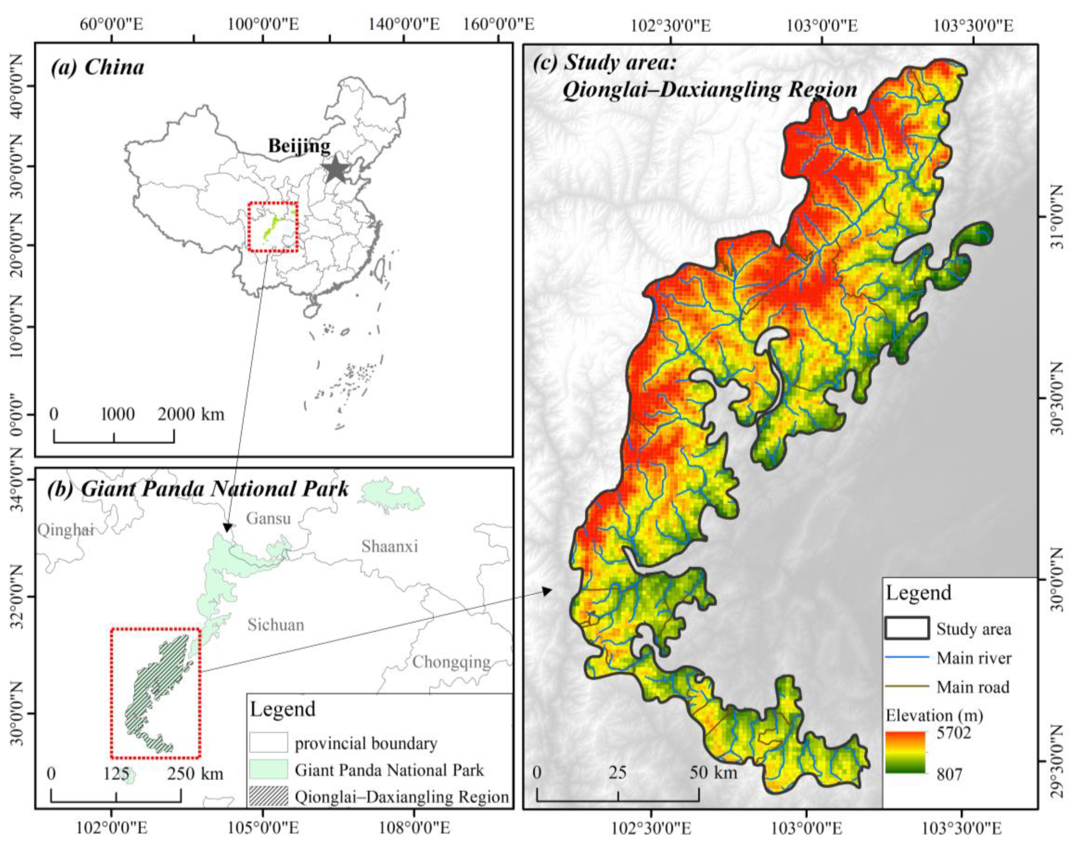
Figure 1. Location of the QDR of the GPNP.
Systems 13 00807 g001
Figure 2. Flowchart illustrating the methodology for evaluating ESV, spatial relationships, and influencing factors using various analytical methods.
Systems 13 00807 g002
Figure 3. Evolution of LULC in the QDR of GPNP from 1990 to 2020.
Systems 13 00807 g003
Figure 4. Spatial pattern of ESV in 1990, 2005, and 2020. ESV levels were classified into five categories using Jenks natural breaks (ArcMap 10.5), which minimizes within-class variance.
Systems 13 00807 g004
Figure 5. Spatial pattern of ESV changes: 1990–2005, 2005–2020, and 1990–2020. Changes in ESV were classified into five categories using Jenks natural breaks (ArcMap 10.5), which minimizes within-class variance.
Systems 13 00807 g005
Figure 6. Temporal trends and spatial correlations among ESVs from 1990 to 2020. * indicates significant correlations at p < 0.05 after Bonferroni correction.
Systems 13 00807 g006
Figure 7. Bivariate Local Moran’s I maps between ESVs from 1990 to 2020 (first-order Queen contiguity, row-standardized weights; 999 permutations). Significance was controlled using Benjamini–Hochberg FDR (q = 0.05); only significant cells are shown (H–H/L–L = synergy; H–L/L–H = trade-off). Results were produced in GeoDa (version 1.6.7).
Systems 13 00807 g007
Figure 8. Correlation matrix of the predictors.
Systems 13 00807 g008
Figure 9. Relative importance of predictors and their impact on ESV in 2020. The bar chart on the left shows the overall importance of each factor, measured by the mean absolute SHAP value. The beeswarm plot on the right illustrates both the magnitude and direction of each feature’s contribution: positive SHAP values indicate a positive effect on ESV, while negative values indicate a negative effect.
Systems 13 00807 g009
Table 1. The average value of ESV per unit area (unit: CNY/ha/yr).
Primary ServicesSecondary ServicesCultivated ForestGrasslandWaterUnused
Provisioning ServicesFood production1060.91267.08246.81461.880.00
Raw material production324.73613.49363.16257.380.00
Water supply−819.75317.32200.974597.640.00
Regulating ServicesGas regulation848.312017.641276.341004.8521.15
Climate regulation447.426037.053374.192267.090.00
Purifying the environment127.991769.071114.153282.52105.77
Hydrological regulation1063.033950.662471.5847,104.6731.73
Supporting ServicesSoil conservation765.802456.601554.881142.3621.15
Maintaining nutrient circulation149.14187.75119.8888.140.00
Biodiversity162.892237.121413.853677.4121.15
Cultural
Services
Aesthetic landscape72.98981.05624.072365.8110.58
Total4203.4620,834.8212,759.8666,249.75211.55
Table 2. Descriptive statistics of variables.
Influencing FactorsVariables (Unit)MinMaxMeanStd. Dev.
ClimaticRainfall (mm)855.362171.121576.33208.19
Sunshine duration (h/yr)1095.932342.581622.45284.04
Temperature (°C)−9.6315.355.504.55
Wind speed (m/s)1.395.623.300.75
TopographicalElevation (m)807.005702.002859.11896.96
Slope (°)0.6768.7928.0312.25
Topographic relief (m)020643.2423.28
SocioeconomicPopulation density (persons/km2)1070669.17105.15
GDP (104 CNY/km2)374266370.42592.17
Table 3. Changes in the area (km2) and share of total area (%) of LULC from 1990 to 2020.
Type199020052020Change
(1990–2020)
Area (km2)Percentage (%)Area
(km2)
Percentage (%)Area
(km2)
Percentage (%)Area (km2)Percentage (%)
Cultivated83.540.8368.890.6882.710.82−0.83−0.99
Forest7462.2074.167877.0578.287869.8278.21407.625.46
Grassland2322.1523.081818.2618.071842.4618.31−479.69−20.66
Water83.980.83119.221.1887.800.873.824.55
Unused109.781.09177.661.77177.691.7767.9161.86
Impervious0.570.011.140.011.740.021.17205.26
Table 4. Evolution of ESV of QDR from 1990 to 2020.
Ecosystem TypeESV (CNY billion)ESV Change
1990200520201990–2020
Cultivated0.350.290.34−0.54%
Forest155.06163.69163.535.46%
Grassland29.6223.2023.51−20.64%
Water5.567.905.824.62%
Unused0.020.040.0461.87%
Total190.61195.11193.231.38%
Table 5. Model performance between random and spatial CV.
Cross-Validation SchemesRMSER2MAPE (%)
Random CV K-fold0.00460.566.98
Spatial Grid Group K-fold (5 × 5)0.00490.467.70
Spatial K-means Group K-fold (k = 16)0.00490.397.92
Disclaimer/Publisher’s Note: The statements, opinions and data contained in all publications are solely those of the individual author(s) and contributor(s) and not of MDPI and/or the editor(s). MDPI and/or the editor(s) disclaim responsibility for any injury to people or property resulting from any ideas, methods, instructions or products referred to in the content.