Abstract
Accurate forecasting of language service demand is essential for language industry planning and resource allocation, yet it remains challenging due to small sample sizes, noisy data, and nonlinear dynamics in industry-level time series. To enhance forecasting accuracy, this study proposes a novel hybrid forecasting framework, called the Sine Cosine Algorithm-optimized wavelet analysis-based new information priority nonhomogeneous discrete grey model (SCA–WA–NIPNDGM). By integrating wavelet-based denoising with the NIPNDGM, the model effectively extracts intrinsic signals and prioritizes recent observations to capture short-term trends while addressing nonlinear parameter estimation via heuristic optimization. Empirical studies are conducted across three high-demand sectors in China from 2000 to 2024, including manufacturing; water conservancy, environmental, and public facilities management; and wholesale and retail. The findings show that the proposed model displays superior performance to 11 benchmark grey models and five optimization algorithms across six evaluation metrics, achieving test Mean Absolute Percentage Error (MAPE) values as low as 1.2%, with strong generalization, stable iterations, and fast convergence. These results underscore its effectiveness in forecasting complex time series and offer valuable insights for language service market planning under emerging AI-driven disruptions.
1. Introduction
Language services serve as an indispensable bridge for promoting international communication, facilitating global trade, fostering cultural exchange, and supporting national initiatives [1]. In an era of accelerating globalization and deepening international interconnectedness, the demand for high-quality and efficient language services has become increasingly critical [2]. Over the past two decades (2000–2024), China’s language service industry has undergone an extraordinary transformation and expansion driven by robust economic growth, the “going out” plan for enterprises, and an influx of foreign investment and collaboration [3]. The total number of language service companies has skyrocketed from approximately 2118 in 2000 to over 124,000 in 2023. This dynamic growth is reflected in the industry’s economic scale: the total output value of China’s language service industry exceeded CNY 198.2 billion in 2023, with the core translation industry itself reaching CNY 70.8 billion and achieving an impressive growth rate of 17.2% over 2021. The industry’s labor force has also grown significantly, employing an estimated 6.8 million people as of the end of 2024. This surge in demand for cross-linguistic services presents both unprecedented opportunities and unique challenges for the sector. The dynamic growth is particularly evident in key economic sectors integral to China’s international engagement. For example, the manufacturing industry has evolved from primarily needing translation for product export localization to requiring sophisticated language services for disseminating international standards, technical documentation for advanced technologies, and global brand building [4]. Similarly, the wholesale and retail sector has been revolutionized by the explosion of cross-border e-commerce, generating immense demand for the translation and localization of product descriptions, marketing content, and customer service communications [5]. The information and communication technology, education and training, and government foreign affairs sectors are identified as having the highest demand for language services, underscoring their critical role in China’s digital and international development. Furthermore, language services are a strategic enabler for major national initiatives. For example, under the Belt and Road Initiative (BRI), a 10% reduction in language barriers has been found to increase China’s trade with BRI countries by 20% and foreign direct investment by 10.61%. This highlights the industry’s crucial function in mitigating communication friction and driving economic gains. The importance of this field is also underscored by national policy, as China’s “14th Five-Year Plan for Digital Economy Development” explicitly lists “language intelligence” as a key emerging field for artificial intelligence, positioning the language service industry at the core of national technological and economic strategy. Understanding and accurately forecasting the development trends within these specific sectors, particularly the number of language service or translation companies serving them, is crucial for resource allocation, language industry planning, and talent cultivation at both industrial and national levels, especially amidst the disruptive impact of AI technology development.
In recent years, the number of language service companies across various industries has shown complex and dynamic growth patterns driven by globalization, technological advancements, and fluctuating market demands. However, the historical data associated with company counts often contains irregular fluctuations and stochastic noise, which may stem from reporting inconsistencies, seasonal effects, and abrupt policy or economic changes. Such noise can obscure the underlying trends and hinder the performance of forecasting models. To solve this problem, it is necessary to preprocess the raw time-series data to extract the intrinsic signal while suppressing random disturbances. A range of denoising techniques has been developed to enhance the quality of time-series data. Traditional methods, such as moving-average filtering [6], offer simplicity but may struggle to handle complex noise structures. More advanced approaches, including singular spectrum analysis [7] and variational-mode decomposition [8], aim to decompose the time series into underlying components, enabling better noise separation. Among these techniques, wavelet analysis (WA) stands out for its ability to perform multiscale decomposition, allowing the signal to be examined simultaneously in both the time and frequency domains [9]. This property makes wavelet-based denoising particularly effective for handling non-stationary and irregular time series, where noise patterns may vary across different time horizons.
Forecasting the number of translation companies is essentially a small-sample problem due to limited and irregular historical data. Grey system theory, designed for systems with insufficient information, is well-suited for such cases. It enables effective pattern extraction and trend forecasting from sparse and uncertain datasets. The foundation of grey prediction modeling is built upon continuous grey models, primarily the classical grey model introduced by Deng [10], which utilizes differential equations to model uncertain systems with limited data. However, it often lacks accuracy when dealing with complex nonlinear dynamics. To improve this, Wu et al. [11] introduced a conformable fractional nonhomogeneous grey model. Xiang et al. [12] proposed an Euler polynomial-driven grey model by driving the Euler polynomial as the grey input. Other improvements include the damping accumulated grey model by Liu et al. [13], which mitigates data randomness. Saxena [14] developed an optimized fractional-overhead power-term polynomial grey model. Nevertheless, continuous grey models exhibit inherent limitations when applied to discrete datasets, as the continuous differential equation approach may introduce structural inconsistencies and reduce model accuracy on volatile or short-term data. To overcome these issues, discrete grey models (DGMs) [15] have been developed, offering improved compatibility with the discrete nature of most real-world time-series data. Early studies focused on nonhomogeneous exponential structures to improve predictive accuracy. For example, Xie and Liu [16] developed a nonhomogeneous exponential DGM for interval grey numbers, and Xie et al. [17] applied a similar model to assess policy shocks in fertility, showing good adaptability to abrupt socioeconomic changes. Later improvements enhanced model structure and flexibility. Liu and Wu [18] proposed an adjacent nonhomogeneous DGM to forecast renewable energy demand. To capture periodicity, Zhou and Ding [19] added seasonal dummy variables to the DGM model, while Ding et al. [20] developed an adaptive DGM with time-varying parameters using genetic algorithms. Structural adaptability was further advanced by Qian and Sui [21], who incorporated nonlinear and periodic terms into the model. Additionally, Zhou et al. [22] addressed monotonicity issues in accumulation by proposing a three-parameter DGM, boosting performance in natural gas demand prediction.
Following the discussion on continuous and discrete grey models, accumulation operators remain key for reducing randomness and capturing system behavior, which smooth raw data to reduce randomness. Traditional first-order accumulation is straightforward but limited in flexibility. To improve this, Wu et al. [23] introduced fractional-order accumulation, enabling better modeling of nonlinear variations. Subsequent studies applied fractional accumulation to environmental and energy forecasting with enhanced accuracy [24,25]. Innovations include the fractional Hausdorff grey model [26] and weakened fractional operators for improved stability [27]. Time-delay and structural adaptations were introduced by Ma et al. [28,29] to further improve flexibility. To address equal weighting of past data, new information priority accumulation was proposed [30] and was later extended by Wang et al. [31] and Guo et al. [32] for improved renewable energy forecasts. Building on these advances, He et al. [33] and Li et al. [34], respectively, proposed structure-adaptive and new information priority generalized grey models. The incorporation of new information priority accumulation introduces nonlinear parameters that require effective optimization to ensure accurate model performance. Traditional optimization methods, such as gradient-based [35] and deterministic algorithms [36], often struggle with issues like local optima entrapment, sensitivity to initial conditions, and computational inefficiency when applied to these nonlinear grey models. To overcome these challenges, heuristic algorithms have gained prominence due to their robust global search capabilities and flexibility. Common examples include the Firefly Algorithm (FFA) [37], Bat Algorithm (BAT) [38], Salp Swarm Algorithm (SSA) [39], Particle Swarm Optimization (PSO) [40], Whale Optimization Algorithm (WOA) [41], and Sine Cosine Algorithm (SCA) [42]. Among these, the SCA stands out for its simple implementation, fast convergence, and strong balance between exploration and exploitation, making it particularly well-suited for optimizing complex nonlinear parameters in grey prediction models [43].
Accurate forecasting of language industry translation companies in the era of AI remains challenging due to the limitations of small sample sizes and noise interference. Although continuous grey models have been extensively studied in general forecasting tasks, their reliance on differential equations may lead to structural inconsistencies and reduced accuracy when applied to discrete, volatile, or short-term data. In contrast, discrete grey models, such as the nonhomogeneous discrete grey model (NDGM), are inherently more compatible with the discrete nature of industry-level time-series data. Moreover, traditional accumulation operators in grey modeling often assign equal weights to all historical data, potentially overlooking recent trends. The new information priority (NIP) accumulation operator offers a promising alternative by emphasizing recent observations, yet its integration with discrete models like the NDGM remains underexplored. Furthermore, the nonlinear nature of this operator introduces complexity into parameter optimization, necessitating the use of robust and efficient heuristic algorithms.
To bridge the above research gaps, this study develops a novel hybrid forecasting framework—the Sine Cosine Algorithm-optimized wavelet analysis-based new information priority nonhomogeneous discrete grey model (SCA–WA–NIPNDGM)—comprising wavelet-based denoising, the new information priority nonhomogeneous discrete grey model, and SCA-based parameter optimization, specifically designed for small-sample, noise-contaminated time-series forecasting. The main contributions of the present study are as follows:
- Wavelet-based time-series denoising is employed as a preprocessing step to extract the intrinsic signal and suppress stochastic fluctuations in the raw data, significantly improving the quality of the input series for grey modeling.
- A novel grey forecasting model, termed the new information priority nonhomogeneous discrete grey model (NIPNDGM) with wavelet analysis, is developed by incorporating the new information priority accumulation operator into the traditional nonhomogeneous discrete grey model. This is the first attempt to combine these two components, enhancing the model’s ability to adapt to recent data trends and capture short-term nonlinear dynamics.
- To address the parameter estimation challenges introduced by the nonlinear nature of the accumulation operator, this study adopts the SCA for automatic parameter optimization. This metaheuristic algorithm ensures global search capability and efficient convergence, enabling the model to achieve high prediction accuracy.
- The proposed hybrid SCA–WA–NIPNDGM is empirically validated on the time series of translation company counts across three representative industries: manufacturing; water conservancy, environmental, and public facilities management; and wholesale and retail. This is the first time it has been applied in the language service industry, and this application provides insight into the sectoral dynamics of language service demand, offering valuable evidence for regional language service planning and targeted policy support.
The remainder of this paper is structured as follows. Section 2 introduces the proposed new information priority nonhomogeneous discrete grey model combined with wavelet analysis, detailing the entire modeling process. Section 3 describes the hyperparameter optimization process using the Sine Cosine Algorithm. Section 4 presents case studies in which the proposed model is applied to forecast the number of translation companies in three key industries. Section 5 presents a discussion of the results. Finally, Section 6 summarizes the main findings and conclusions.
2. New Information Priority Nonhomogeneous Discrete Grey Model with Wavelet Analysis
In this section, the proposed wavelet analysis-based new information priority nonhomogeneous discrete grey model (WA–NIPNDGM) is presented. First, wavelet analysis is employed to denoise the time-series data. Then, a new information priority nonhomogeneous discrete grey model is constructed by incorporating a new information priority accumulation mechanism into the conventional nonhomogeneous discrete grey model.
2.1. Wavelet Analysis for Data Preprocessing
Given that the predictive accuracy of grey models can be affected by stochastic noise, wavelet analysis is employed in this study as a preprocessing filter. The technique functions by decomposing the original time series, allowing for the separation of the core, low-frequency signal (the trend) from high-frequency noise. By providing a smoother, denoised input series to the subsequent grey models, their capacity to accurately capture the underlying development trajectory is enhanced. The entire wavelet denoising procedure was implemented in Python 3.10.12, leveraging the open-source PyWavelets library [44].
To enhance the intrinsic signal-to-noise ratio and mitigate the impact of stochastic volatility within the original time series, a wavelet analysis-based denoising procedure is employed as a preprocessing step. The wavelet transform is exceptionally well-suited for analyzing non-stationary time series owing to its capability for multi-resolution analysis and time-frequency localization [45]. This study utilizes the discrete wavelet transform (DWT) to decompose the signal, isolate noise components, and reconstruct a smoothed series. Let the original time series be denoted as , where n is the total number of observations. The wavelet denoising process is implemented in three primary stages: decomposition, thresholding of detail coefficients, and reconstruction.
Wavelet Decomposition: The original signal is decomposed using the Daubechies 4 (‘db4’) mother wavelet, with the number of decomposition levels set to , a choice balancing signal preservation and noise removal. The DWT at level 2 decomposes the signal into one set of approximation coefficients () and two sets of detail coefficients ( and ). The coefficients represent the low-frequency, coarse structure (i.e., the underlying trend) of the signal. Conversely, and capture higher-frequency details at progressively finer scales, with corresponding to the finest scale, where noise is typically most prominent. The decomposition is formally represented as
Thresholding of Detail Coefficients: Following decomposition, a thresholding strategy is applied exclusively to the detail coefficients to attenuate noise, while the approximation coefficients are preserved unaltered to retain the core signal trend. This study adopts the VisuShrink methodology, which employs a universal threshold [46].
First, the noise standard deviation () is robustly estimated from the detail coefficients at the finest level (). This is based on the common assumption that the highest-frequency coefficients have the lowest signal-to-noise ratio and thus provide the most reliable estimate of the noise level. The estimation uses the median absolute deviation (MAD):
The denominator 0.6745 is a normalization factor that scales the MAD to be a consistent estimator for the standard deviation of an assumed Gaussian noise distribution.
Next, the universal VisuShrink threshold (T) is calculated using the following estimated noise level:
where N is the length of the original signal.
Crucially, this single universal threshold T is then applied to all sets of detail coefficients ( and ) using a soft thresholding rule. This rule shrinks coefficients toward zero, providing a smoother result than hard thresholding. For any given detail coefficient d, the thresholded coefficient is obtained by
where is the signum function. This process yields the sets of denoised detail coefficients, denoted as and .
Signal Reconstruction: Finally, the denoised time series, serving as the clean input sequence for the subsequent grey forecasting models, denoted as , is reconstructed using the inverse discrete wavelet transform (IDWT). The reconstruction combines the original, unmodified approximation coefficients () with the newly thresholded detail coefficients ():
2.2. New Information Priority Nonhomogeneous Discrete Grey Model
New information priority accumulation: The new information priority accumulation assigns greater weight to newer data, reflecting the idea that newer information carries more significance in dynamic systems. This enhances the model’s adaptability and improves forecasting accuracy, especially in non-stationary time series.
Assuming that the non-negative time series is , the first-order new information priority accumulation (1-NIPAGO) for is defined as and can be expressed as
where r is the accumulation-generation parameter. Equation (6) is referred to as new information priority accumulation.
Previous studies have demonstrated that the weight of the “new” 1-NIPAGO series is greater than that of the “old” ones. Analogous to the traditional grey model accumulation generation, can be accumulated and generated multiple times following the above accumulation rule. Through multiple new information operations on , the priority accumulation-generation sequence can be obtained.
Based on the above, assume that the first-order new information priority accumulation (1-NIPAGO) of is , where
It is noteworthy that new information priority accumulation and new information priority inverse accumulation have the following relationship:
Equation (8) is particularly significant when establishing grey forecasting models and calculating prediction values for the original sequence.
NIPNDGM: The nonhomogeneous discrete grey model was proposed by Xie and Liu [47] and is a widely used time-series forecasting method within grey system theory. Unlike traditional continuous grey models, the NDGM operates on discrete-time data and incorporates a nonhomogeneous term to enhance modeling flexibility. This structure allows the NDGM to better capture complex patterns in real-world systems, particularly those characterized by limited and uncertain information. This study integrates the new information priority accumulation with the NDGM to propose the new information priority nonhomogeneous discrete grey model. The modeling details are presented below.
Let the time series processed by wavelet analysis be denoted as , and then the 1-NIPAGO sequence is . The NDGM is given by
and the least squares estimate of its parameters satisfies
where
Equation (11) can be solved using the recursive method. First, the homogeneous form of Equation (11) is given by
where the first-order linear recurrence relation has the general solution
Second, for the nonhomogeneous term , assuming a linear particular solution
substituting into Equation (11) gives
Solving for A and B results in
Finally, the complete solution combines homogeneous and particular components, and is given by
The constant C is determined utilizing the initial condition , and the solution of the NDGM can be obtained as follows:
Finally, the predicted values of the original sequence can be obtained using Equation (8).
3. Hyperparameter Optimization Using the Sine Cosine Algorithm
Based on the proposed WA–NIPNDGM described in Section 2, the nonlinear model hyperparameter r is further optimized using the Sine Cosine Algorithm.
3.1. Optimization Process Using the Sine Cosine Algorithm
To identify the optimal hyperparameters for the proposed WA–NIPNDGM, a hold-out validation scheme is implemented. This approach is well-suited for time-series data, where the temporal order of observations is critical. The core principle involves training the model on the training portion of the time series and subsequently evaluating its predictive accuracy on a separate, succeeding validation segment. The primary criterion for hyperparameter selection is the minimization of the Mean Absolute Percentage Error (MAPE) calculated on this validation set.
The objective function for the hyperparameter optimization process, targeting the minimization of the validation MAPE, is formulated as
where r represents the set of hyperparameters to be optimized. The summation is performed over the m data points in the validation set. denotes the actual value of the j-th observation in the validation set, and is the corresponding forecast generated by the grey model configured with the hyperparameter set r.
The constraints involve
Given that the objective function (Equation (15)) often exhibits a complex, nonlinear relationship with the hyperparameters r, and the constraints are embedded within the grey model’s structural algorithms, conventional numerical optimization algorithms may struggle to find the global optimum. Therefore, this study employs intelligent optimization algorithms to effectively navigate the hyperparameter search space and identify the set r that yields the minimal MAPE on the validation data.
3.2. The Sine Cosine Algorithm
The Sine Cosine Algorithm is a population-based metaheuristic optimization algorithm proposed by Mirjalili in 2016 [48]. The SCA is inspired by the mathematical properties of sine and cosine functions and offers a conceptually simple yet effective approach for solving optimization problems. The algorithm iteratively updates a set of random candidate solutions, guiding them to fluctuate either outward from or toward the current best-known solution to explore and exploit the search space.
In the SCA, each candidate solution (agent) updates its position based on the position of the best solution found so far (destination point). The core position updating mechanism for the j-th dimension of a solution at iteration is defined as follows:
where is the position of the current solution in the j-th dimension at iteration t; is the position of the destination point (i.e., the best solution obtained so far) in the j-th dimension at iteration t; and are random numbers; is a random number in the range , determining how far the movement should be toward or outward from the destination; is a random number in the range , introducing a random weight for the destination to stochastically emphasize () or de-emphasize () its effect; and is a random number in the range , providing an equal probability to switch between the sine and cosine components.
The parameter plays a crucial role in balancing the exploration and exploitation phases of the search process. It dictates the next position’s region, which can be either between the solution and the destination or outside of it. The value of is adaptively updated during the iterations using the following align:
where t is the current iteration, T is the maximum number of iterations, and is a constant. This formulation ensures that decreases linearly from a to 0 over the course of iterations. Larger values of (when t is small) encourage exploration by allowing solutions to move further, potentially outside the space between the current solution and the best solution. Smaller values of (when t is large) promote exploitation by confining the search to regions closer to the best-known solution. This adaptive mechanism allows the SCA to gradually transition from a global search to a more localized refinement.
The SCA begins by initializing a population of random solutions. In each iteration, these solutions are evaluated, the best solution is updated, and then all other solutions update their positions using Equations (16) and (17). This iterative process continues until the maximum number of iterations is met. The pseudocode for applying SCA to optimize WA-NIPNDGM is presented in Algorithm 1.
| Algorithm 1: Hyperparameter optimization of the WA–NIPNDGM using the SCA |
 |
The computational complexity of a model serves as an essential metric for assessing its operational feasibility, directly influencing the model’s runtime. Complexity can be computed via the model’s structure and implementation. For the SCA–WA–NIPNDGM, the overall complexity is primarily determined by the complexities of the SCA, WA, and NIPNDGM. The following parts present a detailed analysis of the computational complexity of each component individually.
Complexity of the SCA: The computational complexity of the SCA is primarily determined by the iterative update of search agent positions and the iterative evaluation of fitness values. The complexity of updating search agent positions is , where denotes the maximum number of iterations, is the population size, and represents the number of parameters to be optimized. The complexity of evaluating the fitness values is , where F is the computational complexity of the fitness evaluation, which in this case depends on the complexity of the WA–NIPNDGM. Therefore, the total complexity of the SCA can be expressed as .
Complexity of WA: The computational complexity of WA is mainly governed by the wavelet decomposition, the thresholding of wavelet coefficients, and the signal reconstruction. The wavelet decomposition, implemented via the wavedec function, essentially performs a multi-level one-dimensional discrete wavelet transform (1D DWT). For an input time series of length n, the computational complexity of a single-level 1D DWT is , as the convolution operations use filters of fixed length independent of n. When the transform is applied up to a specified decomposition level L, the low-frequency approximation coefficients are further decomposed at each stage, resulting in a total operation count of
where L is typically a small constant relative to n. The complexity of thresholding all wavelet coefficients is , as it involves element-wise operations over approximately n coefficients. The complexity of the signal reconstruction is likewise , following the same reasoning as the decomposition. Therefore, the total computational complexity of wavelet denoising can be expressed as
Complexity of the NIPNDGM: The complexity of the NIPNDGM is primarily determined by the following steps:
1. Complexity of 1-NIPAGO: Computing each term according to Equation (6) requires j multiplications and additions. Therefore, calculating all n terms involves a total of operations, resulting in a computational complexity of .
2. Complexity of the least-squares estimate: According to Equations (10) and (11), B denotes the design matrix of size , and Y is the observation vector of size . The computation of the Gram matrix , which is a matrix, involves multiplying a matrix by an matrix. Each element of the resulting matrix requires multiplications and additions, and since there are nine such elements, this step incurs a time complexity of . The subsequent inversion of the matrix is a fixed-size operation; thus, its computational cost is constant: . Next, the product , which yields a vector, involves multiplying a matrix with an vector, entailing three dot products, each of length , resulting in a time complexity of . Finally, the multiplication of the inverse matrix with the vector is a fixed-dimension matrix–vector product, also of constant complexity: . Summing these steps, the overall time complexity for computing is dominated by the two matrix multiplications and thus is linear in the sample size n, that is, . This efficiency arises from the fixed number of parameters (three in this case), meaning the dimensional operations remain constant and only scale with the number of observations. Compared to a general least-squares problem with an design matrix, where the complexity typically scales as , the fixed parameter dimension here simplifies the complexity to linear in n. Therefore, the least-squares estimation problem considered exhibits a computational complexity of , reflecting a scalable and efficient calculation for large sample sizes.
3. Complexity of the time-response solution: For the NIPNDGM, the predicted sequence is given by Equation (13). When computing each term , the exponentiation can be obtained via j successive multiplications, requiring time. The summation involves j multiply–add operations, also incurring time. Since these operations dominate, the total cost for computing the j-th term is proportional to . Summing over all j from 1 to yields the total computational cost:
4. Complexity of the inverse accumulation: Similar to the 1-NIPAGO procedure, the computational complexity is .
In summary, the computational complexity of the NIPNDGM is approximately .
Complexity of the SCA–WA–NIPNDGM: By combining the complexities of the SCA, WA, and NIPNDGM, the overall complexity of the SCA–WA–NIPNDGM can be expressed as
Since the WA–NIPNDGM requires optimization of only a single nonlinear parameter r, , substituting this value yields the simplified complexity
Since grey models are specifically designed to handle small-sample data, n is usually small, and the value of is also typically set to be small, thereby resulting in a relatively low overall computational complexity for the SCA–WA–NIPNDGM.
4. Applications
4.1. Data Collection
For case studies, this study utilized annual data covering the total number of translation companies in three key sectors in China: manufacturing; water conservancy, environmental, and public facilities management; and wholesale and retail. The data were sourced from reports on the development of China’s language services industry and enterprise statistics. The dataset, covering the period from 2000 to 2024, was partitioned for the forecasting tasks. Specifically, annual observations from 2000 to 2020 (21 samples) constituted the training set, employed for initial model fitting. Data from 2021 to 2022 (two samples) formed the validation set, used for tuning model hyperparameters. Finally, data from 2023 to 2024 (two samples) comprised the testing set, utilized to evaluate the out-of-sample forecasting performance of the proposed models.
4.2. Benchmark Models and Algorithms for Comparisons and Evaluation Metrics
To rigorously evaluate the forecasting efficacy of the proposed Sine Cosine Algorithm-optimized wavelet analysis-based new information priority nonhomogeneous discrete grey model, its performance was benchmarked against eleven established grey system models (detailed in Table 1). This comparative analysis aimed to assess their respective capabilities in forecasting highly volatile and nonlinear time-series data. For a fair and robust comparison, the hyperparameters of these benchmark models, where applicable (i.e., excluding the parameter-free GM and DGM), were also systematically optimized using the SCA. It should be noted that as the foundational GM and DGM are parameter-free models, the validation set was not required for hyperparameter tuning. Therefore, the training and validation sets were combined to form a single in-sample set for fitting these two specific models. Furthermore, to investigate the impact of the optimization strategy itself, five distinct intelligent optimization algorithms (as listed in Table 2) were employed to optimize the core wavelet analysis-enhanced NIPNDGM. In the hyperparameter optimization process, the maximum number of iterations T was set to 500. This comparative study of optimization algorithms was conducted to ascertain which method most effectively identifies the optimal hyperparameters, thereby yielding a consistently stable and highly accurate forecasting model. Finally, a comprehensive suite of evaluation metrics, as presented in Table 3, was utilized to quantitatively measure and compare various aspects of the forecasting performance across all developed and benchmark models.

Table 1.
Proposed and benchmark models for comparison, along with their abbreviations.
Table 2.
Comparison of optimization algorithms: models and their abbreviations.
Table 3.
Evaluation metrics for quantitatively measuring and comparing forecasting performance across all developed and benchmark models.
4.3. Forecasting Results and Analysis
4.3.1. Case I: Prediction of the Total Number of Translation Companies in the Manufacturing Sector in China
Figure 1 presents the prediction results for the total number of translation companies in China’s manufacturing industry, encompassing both the training and testing phases. The raw data indicates a fluctuating yet generally increasing trend in the number of translation companies, with notable growth observed toward the latter part of the dataset, particularly between 2015 and 2020. This trend aligns with the broader context of China’s manufacturing industry transformation. As China moves up the global value chain, there is an increasing demand for sophisticated international collaboration, technology transfer, and export-oriented services, all of which necessitate specialized translation and localization. Furthermore, the “Made in China 2025” initiative and the “Belt and Road Initiative” have intensified global engagement, fueling the need for comprehensive translation and language services to facilitate cross-border communication, technical documentation, and regulatory compliance. Among the 12 forecasting models applied, the SCA–WA–NIPNDGM demonstrates a superior ability to describe the underlying dynamics within this time series. In the testing phase, the predicted values from the SCA–WA–NIPNDGM are remarkably close to the raw data compared to those from the other models. This indicates its robust generalization capability and higher accuracy in predicting future trends, reflecting its enhanced adaptability to the evolving landscape of China’s industrial services sector.
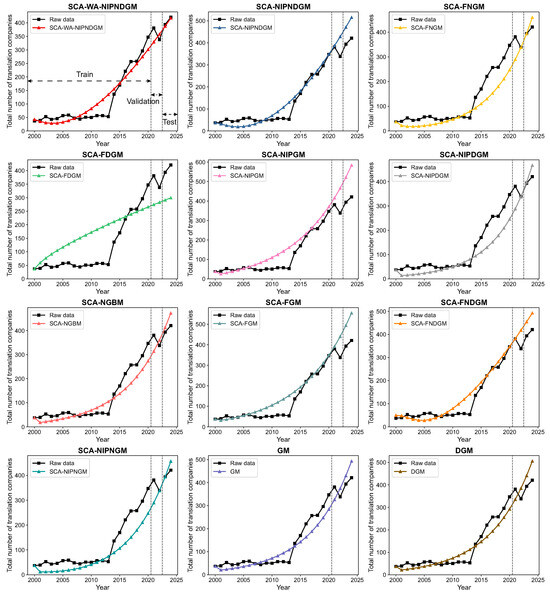
Figure 1.
Predicted total number of translation companies from all models for the manufacturing sector.
The performance evaluation metrics for the validation and test datasets, as detailed in Table 4, further underscore the predictive superiority of the proposed SCA–WA–NIPNDGM, particularly in the testing phase. While several models, such as SCA–FNGM and SCA–NIPNGM, show relatively good performance in the validation phase, the true strength of the SCA–WA–NIPNDGM becomes evident on the test dataset. In the testing phase, it consistently achieves the lowest error metrics across all indicators: MAPE (1.20%), MAE (4.84), MSE (25.95), RMSE (5.09), U1 (0.01), and U2 (0.01). This outstanding performance is significantly superior to that of the 11 comparison models, including the traditional GM and DGM. For instance, its MAPE of 1.20% is substantially lower than that of the next-best models (SCA–NIPNGM at 4.33% and SCA–FNGM at 4.69%) and superior to that of the SCA–NIPNDGM (20.99%) and the traditional GM (13.11%) and DGM (16.07%). The remarkably low U1 and U2 values further confirm that the SCA–WA–NIPNDGM exhibits minimal systematic error and provides highly accurate short-term forecasts on unseen data. This highlights the effectiveness of incorporating wavelet analysis and the improved NIPNDGM structure, optimized by the Sine Cosine Algorithm, in enhancing the model’s performance in capturing complex nonlinear patterns and discrete data characteristics with high precision. The robust performance on the test set validates the SCA–WA–NIPNDGM as a highly reliable and superior forecasting tool for the given time-series data.
Table 4.
Prediction performance metrics for the proposed and benchmark gray models in Case I.
Figure 2 presents the predicted values and convergence curves for six algorithms in Case I. As shown in Figure 2a, during the training phase, the model closely follows the overall trend of the raw data. Although some deviations are observed in the early period, the model adjusts in the mid-to-late stages, aligning more closely with the actual data. In contrast, models such as the PSO–WA–NIPNDGM and WOA–WA–NIPNDGM tend to overestimate values during periods of rapid growth, leading to visible divergence from the observed trend. During the validation phase (2021–2022), the model identifies the transition point between growth and decline and maintains relatively close agreement with the actual trend. Other models, including the SSA–WA–NIPNDGM and WOA–WA–NIPNDGM, show increasing overestimation, with the predicted curves deviating above the observed data. Figure 2b shows the convergence behavior of the optimization algorithms. The model converges within a relatively small number of iterations and exhibits a stable convergence curve. This suggests efficient convergence behavior with reduced susceptibility to local optima. In contrast, the BAT–WA–NIPNDGM and SSA–WA–NIPNDGM show slower convergence and more pronounced fluctuations, indicating potential instability and less effective parameter optimization.
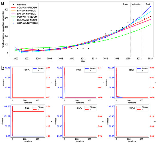
Figure 2.
Predicted values and convergence curves of the six algorithms in Case I. (a) Prediction results of the six algorithms compared to the raw data; (b) Convergence curves of the fitness and the hyperparameters for each algorithm.
The metrics for the six algorithms in the validation and test phases of Case I are listed in Table 5. In the validation phase, the SCA–WA–NIPNDGM achieves an MAPE of 9.75%, which is only marginally higher than that of the FFA–WA–NIPNDGM and BAT–WA–NIPNDGM (both at 9.38%) but significantly higher than that of the PSO–WA–NIPNDGM (27.71%), SSA–WA–NIPNDGM (11.56%), and WOA–WA–NIPNDGM (13.61%). More notably, the SCA–WA–NIPNDGM yields the lowest RMSE (39.17) and MSE (1534.43) among all models, indicating higher stability and accuracy. Moreover, it attains the best performance on Theil’s inequality coefficients, with U1 = 0.06 and U2 = 0.11, reflecting superior forecasting precision and lower bias. In the test phase, the proposed model demonstrates an even more prominent advantage. The SCA–WA–NIPNDGM achieves the lowest MAPE (1.20%), MAE (4.84), MSE (25.95), and RMSE (5.09), far surpassing all other models. For example, compared to the FFA–WA–NIPNDGM and BAT–WA–NIPNDGM, which both attain RMSE values above 34, and the PSO–WA–NIPNDGM with an RMSE of 95.90, the SCA-based model shows a remarkable reduction in prediction error. Additionally, the SCA–WA–NIPNDGM achieves U1 = 0.01 and U2 = 0.01, the lowest among all compared models, confirming its exceptional generalization capability and robustness in unseen data scenarios. Overall, the empirical results indicate that the SCA-based model outperforms all other hybrid models across both the validation and test sets, particularly excelling in minimizing error and enhancing predictive reliability.
Table 5.
Validation and test metrics for the six algorithms in Case I.
4.3.2. Case II: Prediction of Total Number of Translation Companies in the Water Conservancy, Environmental, and Public Facilities Management Sector in China
Figure 3 illustrates the prediction results for the total number of translation companies operating within China’s water conservancy, environmental, and public facilities management sector, covering both the training and testing phases. The raw data reveals a period of relatively modest growth in the initial years, followed by a significant acceleration, particularly from around 2017 onward, and a notably steep increase in the most recent years (2021–2022). This pronounced upward trend likely reflects China’s intensified focus and investment in environmental protection, sustainable water resource management, and the development of public infrastructure as national priorities. Initiatives such as the “Beautiful China” policy, extensive environmental regulations, and large-scale infrastructure projects necessitate substantial international collaboration, technology exchange, and a high volume of technical documentation and regulatory communication, thereby driving the demand for specialized translation services. Among the twelve forecasting models evaluated, the proposed SCA–WA–NIPNDGM adeptly captures this evolving dynamic. As observed in the testing phase (2023–2024), the predictions from the SCA–WA–NIPNDGM closely follow the sharp growth trajectory of the raw data, indicating its strong capability to model the rapidly expanding demand within this specialized service sector.
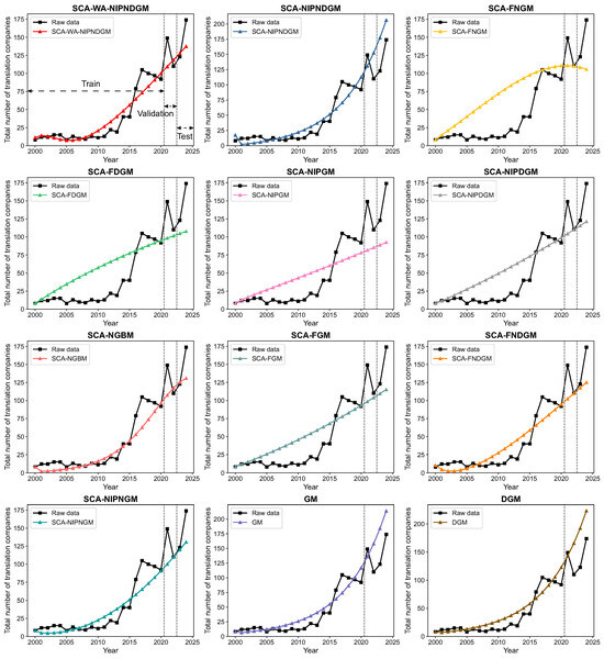
Figure 3.
Predicted total number of translation companies from all models for the water conservancy, environmental, and public facilities management sector.
The comprehensive performance evaluation metrics for both the validation and test datasets, as presented in Table 6, further substantiate the superior predictive accuracy of the SCA–WA–NIPNDGM, especially for forecasts on the test set. While models like the SCA–NGBM and SCA-NIPNGM exhibit competitive performance, the SCA–WA–NIPNDGM consistently outperforms all other models in the crucial test phase across all error indicators. Specifically, on the test dataset, the SCA–WA–NIPNDGM achieves the lowest MAPE (12.57%), MAE (20.81), MSE (680.86), RMSE (26.09), U1 (0.09), and U2 (0.17). This performance is markedly better than that of the next-best models on the test set, such as the SCA–NGBM (MAPE 13.39%, MAE 22.76) and SCA-NIPNGM (MAPE 13.52%, MAE 22.96), and significantly surpasses that of traditional models like the GM (MAPE 36.37%) and DGM (MAPE 42.40%). The exceptionally low U1 (0.09) and U2 (0.17) values for the SCA–WA–NIPNDGM affirm its minimal systematic error and its proficiency in delivering highly accurate short-term forecasts on previously unseen data. This robust performance underscores the efficacy of integrating wavelet analysis for data preprocessing with the enhanced NIPNDGM structure, optimized by the Sine Cosine Algorithm, in capturing the complex, nonlinear, and discrete characteristics inherent in the time-series data of this rapidly growing sector.
Table 6.
Prediction performance metrics for the proposed and benchmark grey models in Case II.
Figure 4 illustrates the temporal prediction performance of six hybrid forecasting models compared with the original data over the period 2000–2024, with the data segmented into training (2000–2020), validation (2021–2022), and test (2023–2024) phases. From Figure 4a, the predicted results indicate that the SCA–WA–NIPNDGM maintains close alignment with the observed data across most of the time series. Although some discrepancies appear in the early years, the model captures the nonlinear upward trend effectively, particularly from 2010 onward. Notably, the predicted curves of the FFA–WA–NIPNDGM and BAT–WA–NIPNDGM are nearly identical to those of the SCA-based model throughout the entire period, suggesting that these three models exhibit similar fitting behavior under this dataset and optimization framework. In contrast, the PSO–WA–NIPNDGM, SSA–WA–NIPNDGM, and WOA–WA–NIPNDGM show larger deviations from the actual trend, with consistent overestimation during periods of rapid growth or turning points. The SCA-based model, however, demonstrates stable performance even during the test phase and yields the smallest deviation from the observed values in the final year. This reflects its stronger generalization ability and more accurate trend tracking compared to other algorithms. As shown in Figure 4b, although the final forecasting results of the SCA–WA–NIPNDGM, BAT–WA–NIPNDGM, and SSA–WA–NIPNDGM are similar in magnitude, their optimization behavior differs considerably. The BAT–WA–NIPNDGM and SSA–WA–NIPNDGM exhibit slower convergence and more pronounced oscillations during iteration, indicating less stable optimization dynamics. In contrast, the SCA–WA–NIPNDGM converges more quickly and smoothly, suggesting relatively higher optimization efficiency and stability. When both prediction accuracy and convergence characteristics are considered, the SCA-based model demonstrates more consistent performance.
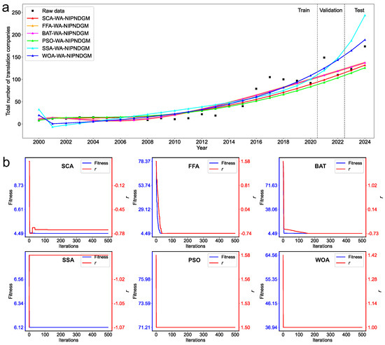
Figure 4.
Predicted values and convergence curves of the six algorithms in Case II. (a) Prediction results of the six algorithms compared to the raw data; (b) Convergence curves of the fitness and the hyperparameters for each algorithm.
The validation and test metrics for the six algorithms in Case II are summarized in Table 7. In the validation phase, SCA–WA–NIPNDGM achieves an MAPE of 17.24%, which is notably lower than that of the PSO–WA–NIPNDGM (21.69%), SSA–WA–NIPNDGM (26.78%), and WOA–WA–NIPNDGM (23.31%). It also attains the lowest MAE (24.14) and RMSE (28.63), matched only by the FFA–WA–NIPNDGM and BAT–WA–NIPNDGM, both of which exhibit identical performance across all error metrics. Regarding Theil’s inequality coefficients, the SCA–WA–NIPNDGM reports U1 = 0.12 and U2 = 0.22, slightly better than the values obtained by most other models, except for the WOA–WA–NIPNDGM, which yields U1 = 0.11. In the test phase, the SCA–WA–NIPNDGM continues to exhibit superior performance. It achieves the lowest MAPE (12.57%), MAE (20.81), and RMSE (26.09), indicating enhanced generalization ability on out-of-sample data. Although the FFA–WA–NIPNDGM and BAT–WA–NIPNDGM also exhibit nearly identical results, the SCA-based model obtains the lowest MSE (680.86), as well as the most favorable Theil’s U1 (0.09) and U2 (0.17), reflecting minimal deviation and reduced forecasting bias. In contrast, the SSA–WA–NIPNDGM yields significantly higher error levels, with an MAPE of 45.97% and an RMSE of 66.82, indicating poor adaptability in the test scenario.
Table 7.
Validation and test metrics for the six algorithms in Case II.
4.3.3. Case III: Prediction of the Total Number of Translation Companies in the Wholesale and Retail Sector in China
Figure 5 shows the prediction results for the total number of translation companies serving China’s wholesale and retail sector, covering both the training and testing phases. The raw data show a dramatic growth trajectory, beginning with a modest base and accelerating exponentially, especially in the later years of the observed period. This surge is directly attributable to the explosive boom in cross-border e-commerce, which has transformed the wholesale and retail landscape. This has created a massive and continuous demand for the translation and localization of product descriptions, marketing content, customer support communications, and regulatory information, often requiring high-volume, high-frequency, rapid-turnaround language services. The proposed SCA–WA–NIPNDGM demonstrates exceptional proficiency in tracking this steep, nonlinear growth. In the testing phase, its predictions align closely with the actual data points, effectively modeling the sector’s rapid expansion without the significant overestimation seen in many competing models.
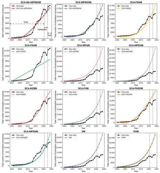
Figure 5.
Predicted number of translation companies from all models for the wholesale and retail sector.
The superior predictive capability of the SCA–WA–NIPNDGM is quantitatively confirmed by the performance metrics detailed in Table 8, particularly in the demanding test phase. On the test dataset, the SCA–WA–NIPNDGM unequivocally exhibits the best performance, recording the lowest error values across all six indicators: MAPE (8.65%), MAE (1093.84), MSE (1,233,627.24), RMSE (1110.69), U1 (0.05), and U2 (0.09). The MAPE of 8.65% represents a dramatic improvement over the next-best performers, such as the SCA–NGBM (22.23%) and SCA–NIPNGM (24.01%). Furthermore, it starkly outperforms its direct predecessor, the SCA–NIPNDGM (43.60%), and traditional benchmark models like the GM (139.08%) and DGM (142.15%), highlighting the significant limitations of these other models in handling such volatile, high-growth data. The remarkably low Theil’s U statistics, U1 (0.05) and U2 (0.09), further validate the model’s high precision, indicating minimal systematic error and a strong ability to forecast future values accurately. This robust and superior performance on the test set confirms that the integration of wavelet analysis for denoising, combined with the refined NIPNDGM structure and optimization by the Sine Cosine Algorithm, provides a powerful and reliable tool for forecasting in sectors characterized by rapid, exponential growth and high volatility.
Table 8.
Prediction performance metrics for the proposed and benchmark grey models in Case III.
Figure 6 presents the predicted and actual values from 2000 to 2024 across the six hybrid models. Overall, the proposed SCA–WA–NIPNDGM demonstrates a high degree of alignment with the observed data throughout the training (2000–2020), validation (2021–2022), and test (2023–2024) phases. Its forecast trajectory closely follows the trend of the original series, particularly in capturing key inflection points and growth patterns with minimal deviation. In contrast, several alternative models—most notably the PSO–WA–NIPNDGM, SSA–WA–NIPNDGM, and WOA–WA–NIPNDGM—exhibit substantial divergence from the actual data, particularly in the early training years. These models generate negative predictions for certain years (e.g., PSO–WA–NIPNDGM for 2001–2003), which are not physically plausible given the nature of the data, suggesting instability in their estimation under sparse or volatile conditions. Moreover, the trajectories of these models often show abrupt fluctuations or overestimated peaks, especially from 2021 onward. Although the FFA–WA–NIPNDGM and BAT–WA–NIPNDGM produce predictions similar to those of the SCA–WA–NIPNDGM in the mid-to-late periods (2010-2024), they tend to systematically underestimate the values during the earlier part of the series and lag behind in capturing the steep increases observed in the ground truth. By comparison, the SCA–WA–NIPNDGM maintains better consistency across all time segments, with smaller residuals and fewer directional mismatches relative to the observed data curve. As shown in Figure 6b, most optimization algorithms exhibit rapid convergence behavior, reaching stable objective values within a relatively small number of iterations. An exception is observed in the case of the BAT–WA–NIPNDGM, which demonstrates significantly slower convergence. The BAT-based model requires more iterations to stabilize and displays noticeable oscillations during the early stages of the optimization process, indicating reduced convergence efficiency and potential sensitivity to initial parameter settings.
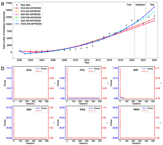
Figure 6.
Predicted values and convergence curves of the six algorithms in Case III. (a) Prediction results of the six algorithms compared to the raw data; (b) Convergence curves of the fitness and the hyperparameters for each algorithm.
The validation and test metrics for the six algorithms are summarized in Table 9. In the validation phase, the SCA–WA–NIPNDGM achieves an MAPE of 8.25%, which is substantially lower than that of the FFA–WA–NIPNDGM (12.02%), BAT–WA–NIPNDGM (12.02%), PSO–WA–NIPNDGM (12.52%), and WOA–WA–NIPNDGM (12.52%). It also attains the lowest MAE (924.62) and RMSE (1187.72), followed by SSA–WA–NIPNDGM with MAE = 1119.83 and RMSE = 1279.04. In terms of Theil’s inequality coefficients, the SCA–WA–NIPNDGM reports U1 = 0.06 and U2 = 0.11, which are among the most favorable across all models, matched only by those of the SSA–WA–NIPNDGM (U1 = 0.06, U2 = 0.12). In the test phase, the SCA–WA–NIPNDGM continues to demonstrate strong predictive capability. It achieves the lowest MAPE (8.65%) and MAE (1093.84), along with the smallest RMSE (1110.69), outperforming all other models. While the SSA–WA–NIPNDGM also shows relatively low errors (MAPE = 9.09%, RMSE = 1241.77), its performance remains slightly inferior to that of the SCA-based model. In addition, the SCA–WA–NIPNDGM achieves the lowest MSE (1,233,627.24) and favorable values of U1 = 0.05 and U2 = 0.09, indicating reduced forecasting bias and deviation. In contrast, the PSO–WA–NIPNDGM and WOA–WA–NIPNDGM exhibit considerably higher error levels in both the validation and test phases, with test-phase RMSE values exceeding 2600 and MAPE values close to 20%, reflecting reduced generalization ability. These results indicate that, among the six models, the SCA–WA–NIPNDGM offers the most stable and accurate forecasting performance across both datasets.
Table 9.
Validation and test metrics for the six algorithms in Case III.
5. Discussion
This section provides an in-depth analysis of the forecasting results, with a particular focus on the comparative performance of the proposed hybrid model against its non-wavelet-denoised counterpart and other benchmark models. The discussion also delves into the implications of the findings for understanding and predicting the development trends within China’s language service industry.
5.1. Effectiveness of Integrating Wavelet Analysis in Enhancing NIPNDGM Forecasting Accuracy
Experiments of the NIPNDGM with and without wavelet analysis under identical SCA-derived optimal hyperparameters were conducted to further investigate the effectiveness of wavelet analysis. The results show that the integration of wavelet analysis as a data preprocessing technique with the SCA-optimized NIPNDGM yields a consistent improvement in forecasting accuracy across all three investigated sectors of China’s language services. As illustrated in Figure 7, this enhancement is evident both in the alignment of predicted values with actual data and in the quantitative evaluation metrics, particularly during the testing phase.
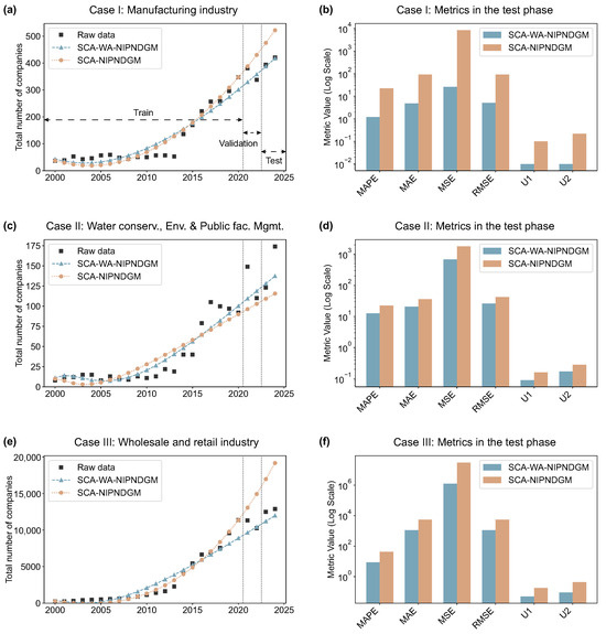
Figure 7.
Comparisons of the SCA-optimized NIPNDGM models with and without wavelet analysis. (a) Prediction results and (b) test-phase metrics for the manufacturing sector; (c) prediction results and (d) test-phase metrics for the water conservancy, environmental, and public facilities management sector; (e) prediction results and (f) test-phase metrics for the wholesale and retail sector.
In Case I, focusing on the manufacturing industry (Figure 7a), the SCA–WA–NIPNDGM, utilizing an optimal hyperparameter , more closely tracks the observed number of translation companies, especially in the validation and testing periods, compared to the SCA–NIPNDGM. While both models capture the general upward trend, the wavelet-enhanced model exhibits a smoother and more responsive predicted curve. This qualitative observation is also supported by the test phase metrics (Figure 7b). The SCA–WA–NIPNDGM achieved a remarkably low MAPE of 1.20%, MAE of 4.84, MSE of 25.95, and RMSE of 5.09. In contrast, the SCA–NIPNDGM, using the same SCA-optimized hyperparameter, yielded significantly higher errors in the test phase (MAPE: 22.27%, MAE: 90.97, MSE: 8374.29, RMSE: 91.51). The Theil’s U1 and U2 statistics further underscore this superiority, with values of 0.006 and 0.012 for the SCA–WA–NIPNDGM, compared to 0.101 and 0.224 for the SCA–NIPNDGM, respectively, indicating a substantially better predictive fit for the wavelet-integrated model. A similar pattern of improved performance is observed in Case II, which analyzes the water conservancy, environmental, and public facilities management sector (optimal ). As depicted in Figure 7c, the SCA–WA–NIPNDGM again provides a more accurate representation of the historical data trajectory, particularly in navigating the fluctuations present in the series. The corresponding test-phase metrics (Figure 7d) reveal a clear advantage for the wavelet-denoised model: the MAPE (12.57% vs. 22.35%), MAE (20.81 vs. 36.03), MSE (680.86 vs. 1794.86), and RMSE (26.09 vs. 42.37) values are all substantially lower for the SCA–WA–NIPNDGM. This suggests that the denoising process effectively filters out noise components that otherwise hamper the predictive capability of the standard NIPNDGM. Finally, in Case III, examining the wholesale and retail industry (optimal ), the benefits of wavelet preprocessing are again pronounced (Figure 7e,f). This sector’s data exhibits a more exponential growth pattern, and the SCA–WA–NIPNDGM demonstrates a superior ability to capture this dynamic. In the test phase, the SCA–WA–NIPNDGM achieves an MAPE of 8.65%, while the SCA–NIPNDGM yields an MAPE of 42.27%.
Across all three cases, the application of wavelet analysis prior to grey model forecasting, under identical SCA-derived optimal hyperparameters, consistently leads to more accurate and reliable out-of-sample predictions. This underscores the efficacy of wavelet denoising in extracting a clearer signal from raw time-series data, thereby enabling the NIPNDGM to more effectively capture the intrinsic developmental trends of translation company numbers within these diverse sectors of the Chinese economy.
5.2. Policy Implications for the Development of China’s Language Service Industry
The forecasting results obtained from the SCA–WA–NIPNDGM provide quantitative foresight into the developmental trajectory of key segments within China’s language service industry. The model’s demonstrated accuracy in predicting the number of translation companies in the manufacturing; water conservancy, environmental, and public facilities management; and wholesale and retail sectors offers valuable insights into the ongoing development and future trajectory of China’s language service industry. The empirical data and the model’s projections confirm that the sector’s expansion is intrinsically linked to China’s broader economic internationalization. The exponential growth in translation enterprises serving the wholesale and retail sector (from 247 in 2000 to 12888 in 2024) directly mirrors the boom in cross-border e-commerce. Similarly, the steady increase in firms supporting the manufacturing sector (from 37 to 421) reflects its evolution from requiring basic product localization to needing sophisticated language services for international standard-setting and technology exports. Even the consistent growth (from 8 to 174) in a niche area like the water conservancy, environmental, and public facilities management sector points to sustained demand driven by international cooperation on infrastructure and sustainability projects.
While China’s language service sector has achieved significant scale, evidenced by the growth to 6.808 million practitioners and a vast number of enterprises, its future trajectory is increasingly defined by the paradoxical influence of large AI models [58]. These models create a paradigm-shifting opportunity for the industry to provide high-value strategic communication services, yet they concurrently introduce formidable challenges related to talent displacement, data security, and the ethical integrity of AI-generated content. Based on our findings, the following policy recommendations are proposed:
- The lack of standardized data at both regional and sectoral levels remains a major obstacle to accurate forecasting in the language service industry. Establishing a unified statistical reporting standard, alongside secure and accessible data repositories, would enhance the reliability and geographic coverage of analyses.
- Government and industry associations should establish a unified statistical framework and create secure, high-quality language data repositories. This dual initiative would support accurate policymaking and enable Chinese enterprises to safely train domain-specific AI models, thereby enhancing global competitiveness.
- To support the small and medium-sized enterprises that constitute the majority of firms in the industry, policies should facilitate the ethical and effective adoption of AI through targeted measures. These include subsidies for privacy-compliant tools, AI literacy workshops, and funding for secure, pre-trained models to help these enterprises meet modern trade demands while mitigating data security risks.
- To ensure responsible innovation, industry associations, with governmental support, should develop a dedicated AI governance framework. This framework must establish a clear ethical code of conduct addressing data privacy, transparency, accountability for AI output, and intellectual property rights, thereby fostering trust and sustainable industry growth.
6. Conclusions
In the present study, a wavelet analysis-based new information priority nonhomogeneous discrete grey model was developed, in which the hyperparameter r is optimized using the Sine Cosine Algorithm, to enhance forecasting accuracy within China’s language service industry. Three distinct case studies were examined, focusing on the manufacturing; water conservancy, environmental, and public facilities management; and wholesale and retail sectors, to evaluate the proposed model against several benchmark grey system models. The results demonstrate that the SCA–WA–NIPNDGM outperformed traditional grey models and other optimized algorithms, particularly in minimizing testing errors. Notably, the model’s MAPE values were significantly lower, indicating its superior capability in capturing the complex trends inherent in the datasets. For instance, in the manufacturing sector, the SCA–WA–NIPNDGM achieved an MAPE of 1.20%, while other models exhibited substantially higher errors, reflecting the model’s robustness and adaptability to market fluctuations. Moreover, the integration of wavelet analysis proved to be a critical enhancement, effectively filtering noise and allowing the model to extract clearer signals from the raw data. This finding underscores the importance of employing advanced data preprocessing techniques in predictive modeling frameworks, particularly in dynamic sectors such as translation services. As the sector continues to evolve in response to global economic shifts, the findings suggest that the proposed model can serve as an effective tool for decision-making and planning in the translation services market. Future research could explore the applicability of this model across other sectors, further contributing to the development of sophisticated forecasting methods in complex, data-driven environments. Additionally, to address the prevalence of data gaps in this field, the NIPNDGM could be extended to a non-equidistant framework to handle unevenly spaced or missing data, thereby increasing its practical applicability.
Author Contributions
Conceptualization, X.L. and X.M.; Methodology, X.M.; Investigation, X.L.; Resources, X.L.; Data curation, X.L.; Writing—original draft, X.L.; Writing—review & editing, X.L. and X.M.; Supervision, X.M. All authors have read and agreed to the published version of the manuscript.
Funding
This research was funded by the project of Guangdong Provincial Key Research Institute of Humanities and Social Sciences/Center for Translation Studies at Guangdong University of Foreign Studies, “Research on the Development of Interpreting Strategic Competence in Student Interpreters” (Project No.: CTS202111).
Data Availability Statement
The original contributions presented in this study are included in the article. Further inquiries can be directed to the corresponding author.
Conflicts of Interest
The author declare no conflicts of interest.
References
- Wang, J. Exploring Chinese Economic Discourse and Translation Strategies in the Era of AI: A Digital-Tech Approach. Commun. Across Borders Transl. Interpret. 2024, 4, 13–19. [Google Scholar]
- Gao, Y.; La, T. A Frontier Exploration of Translation Industry Research in the Age of Artificial Intelligence. J. Humanit. Arts Soc. Sci. 2024, 8, 2852–2862. [Google Scholar] [CrossRef]
- Kunkel, S.; Matthess, M.; Xue, B.; Beier, G. Industry 4.0 in sustainable supply chain collaboration: Insights from an interview study with international buying firms and Chinese suppliers in the electronics industry. Resour. Conserv. Recycl. 2022, 182, 106274. [Google Scholar] [CrossRef]
- Huang, X. The roles of competition on innovation efficiency and firm performance: Evidence from the Chinese manufacturing industry. Eur. Res. Manag. Bus. Econ. 2023, 29, 100201. [Google Scholar] [CrossRef]
- Tang, W.; Li, G. Enhancing competitiveness in cross-border e-commerce through knowledge-based consumer perception theory: An exploration of translation ability. J. Knowl. Econ. 2024, 15, 14935–14968. [Google Scholar] [CrossRef]
- Zhao, Y.; Huang, S.; Wang, X.; Shi, J.; Yao, S. Energy management with adaptive moving average filter and deep deterministic policy gradient reinforcement learning for fuel cell hybrid electric vehicles. Energy 2024, 312, 133395. [Google Scholar] [CrossRef]
- Le, T.T.; Abed-Meraim, K.; Trung, N.L.; Ravier, P.; Buttelli, O.; Holobar, A. Tensor-based higher-order multivariate singular spectrum analysis and applications to multichannel biomedical signal analysis. Signal Process. 2026, 238, 110113. [Google Scholar] [CrossRef]
- Yang, W.; Zhang, H.; Wang, J.; Hao, Y. A new perspective on non-ferrous metal price forecasting: An interpretable two-stage ensemble learning-based interval-valued forecasting system. Adv. Eng. Inform. 2025, 65, 103267. [Google Scholar] [CrossRef]
- Moni, M.; Sreeraj; Sankararaman, S. Unveiling the interdependency of cryptocurrency and Indian stocks through wavelet and nonlinear time series analysis: An Econophysics approach. Phys. Stat. Mech. Its Appl. 2025, 670, 130643. [Google Scholar] [CrossRef]
- Deng, J.-L. Control problems of grey systems. Syst. Control Lett. 1982, 1, 288–294. [Google Scholar] [CrossRef]
- Wu, W.; Ma, X.; Zhang, Y.; Li, W.; Wang, Y. A novel conformable fractional non-homogeneous grey model for forecasting carbon dioxide emissions of BRICS countries. Sci. Total Environ. 2020, 707, 135447. [Google Scholar] [CrossRef] [PubMed]
- Xiang, X.; Ma, X.; Ma, M.; Wu, W.; Yu, L. Research and application of novel Euler polynomial-driven grey model for short-term PM10 forecasting. Grey Syst. Theory Appl. 2021, 11, 498–517. [Google Scholar] [CrossRef]
- Liu, L.; Chen, Y.; Wu, L. The damping accumulated grey model and its application. Commun. Nonlinear Sci. Numer. Simul. 2021, 95, 105665. [Google Scholar] [CrossRef]
- Saxena, A. Optimized Fractional Overhead Power Term Polynomial Grey Model (OFOPGM) for market clearing price prediction. Electr. Power Syst. Res. 2023, 214, 108800. [Google Scholar] [CrossRef]
- Xie, N.; Liu, S. Research on Discrete Grey Model and Its Mechanism. In Proceedings of the 2005 IEEE International Conference on Systems, Man and Cybernetics, Waikoloa, HI, USA, 12 October 2005; Volume 1, pp. 606–610. [Google Scholar]
- Xie, N.; Liu, S. Interval grey number sequence prediction by using non-homogenous exponential discrete grey forecasting model. J. Syst. Eng. Electron. 2015, 26, 96–102. [Google Scholar] [CrossRef]
- Xie, N.; Wang, R.; Chen, N. Measurement of shock effect following change of one-child policy based on grey forecasting approach. Kybernetes 2018, 47, 559–586. [Google Scholar] [CrossRef]
- Liu, L.; Wu, L. Forecasting the renewable energy consumption of the European countries by an adjacent non-homogeneous grey model. Appl. Math. Model. 2021, 89, 1932–1948. [Google Scholar] [CrossRef]
- Zhou, W.; Ding, S. A novel discrete grey seasonal model and its applications. Commun. Nonlinear Sci. Numer. Simul. 2021, 93, 105493. [Google Scholar] [CrossRef]
- Ding, S.; Li, R.; Tao, Z. A novel adaptive discrete grey model with time-varying parameters for long-term photovoltaic power generation forecasting. Energy Convers. Manag. 2021, 227, 113644. [Google Scholar] [CrossRef]
- Qian, W.; Sui, A. A novel structural adaptive discrete grey prediction model and its application in forecasting renewable energy generation. Expert Syst. Appl. 2021, 186, 115761. [Google Scholar] [CrossRef]
- Zhou, W.; Zeng, B.; Wu, Y.; Wang, J.; Li, H.; Zhang, Z. Application of the three-parameter discrete direct grey model to forecast Chinas natural gas consumption. Soft Comput. 2023, 27, 3213–3228. [Google Scholar] [CrossRef]
- Wu, L.; Liu, S.; Yao, L.; Yan, S.; Liu, D. Grey system model with the fractional order accumulation. Commun. Nonlinear Sci. Numer. Simul. 2013, 18, 1775–1785. [Google Scholar] [CrossRef]
- Wu, L.F.; Liu, S.F.; Cui, W.; Liu, D.L.; Yao, T.X. Non-homogenous discrete grey model with fractional-order accumulation. Neural Comput. Appl. 2014, 25, 1215–1221. [Google Scholar] [CrossRef]
- Hao, Y.; Wang, X.; Wang, J.; Yang, W. A new perspective of wind speed forecasting: Multi-objective and model selection-based ensemble interval-valued wind speed forecasting system. Energy Convers. Manag. 2024, 299, 117868. [Google Scholar] [CrossRef]
- Chen, Y.; Wu, L.; Liu, L.; Zhang, K. Fractional Hausdorff grey model and its properties. Chaos Solitons Fractals 2020, 138, 109915. [Google Scholar] [CrossRef]
- Zhu, H.; Liu, C.; Wu, W.Z.; Xie, W.; Lao, T. Weakened fractional-order accumulation operator for ill-conditioned discrete grey system models. Appl. Math. Model. 2022, 111, 349–362. [Google Scholar] [CrossRef]
- Ma, X.; He, Q.; Li, W.; Wu, W. Time-delayed fractional grey Bernoulli model with independent fractional orders for fossil energy consumption forecasting. Eng. Appl. Artif. Intell. 2025, 155, 110942. [Google Scholar] [CrossRef]
- Ma, X.; Yuan, H.; Ma, M.; Wu, L. A novel fractional Bessel grey system model optimized by Salp Swarm Algorithm for renewable energy generation forecasting in developed countries of Europe and North America. Comput. Appl. Math. 2025, 44, 98. [Google Scholar] [CrossRef]
- Zhou, W.; Zhang, H.; Dang, Y.; Wang, Z. New information priority accumulated grey discrete model and its application. Chin. J. Manag. Sci. 2017, 25, 140–148. [Google Scholar]
- Wang, Y.; Yang, Z.; Zhou, Y.; Liu, H.; Yang, R.; Sun, L.; Sapnken, F.E.; Narayanan, G. A novel structure adaptive new information priority grey Bernoulli model and its application in China’s renewable energy production. Renew. Energy 2025, 239, 122052. [Google Scholar] [CrossRef]
- Guo, X.; Dang, Y.; Ding, S.; Cai, Z.; Li, Y. A new information priority grey prediction model for forecasting wind electricity generation with targeted regional hierarchy. Expert Syst. Appl. 2024, 252, 124199. [Google Scholar] [CrossRef]
- He, X.; Wang, Y.; Zhang, Y.; Ma, X.; Wu, W.; Zhang, L. A novel structure adaptive new information priority discrete grey prediction model and its application in renewable energy generation forecasting. Appl. Energy 2022, 325, 119854. [Google Scholar] [CrossRef]
- Li, K.; Xiong, P.; Wu, Y.; Dong, Y. Forecasting greenhouse gas emissions with the new information priority generalized accumulative grey model. Sci. Total Environ. 2022, 807, 150859. [Google Scholar] [CrossRef]
- Pollini, N. A multi-objective gradient-based approach for prestress and size optimization of cable domes. Int. J. Solids Struct. 2025, 320, 113476. [Google Scholar] [CrossRef]
- Wan, Z.; Zhang, J.; Sun, X.; Zhang, Z. Efficient deterministic algorithms for maximizing symmetric submodular functions. Theor. Comput. Sci. 2025, 1046, 115312. [Google Scholar] [CrossRef]
- Yousif, A. An Adaptive Firefly Algorithm for Dependent Task Scheduling in IoT-Fog Computing. Cmes Comput. Model. Eng. Sci. 2025, 142, 2869–2892. [Google Scholar] [CrossRef]
- Masood, M.; Fouad, M.M.; Kamal, R.; Aurangzeb, K.; Aslam, S.; Ullah, Z.; Glesk, I. Enhanced optimisation of MPLS network traffic using a novel adjustable Bat algorithm with loudness optimizer. Results Eng. 2025, 26, 104774. [Google Scholar] [CrossRef]
- Sowmiya, M.; Banu Rekha, B.; Malar, E. Optimized heart disease prediction model using a meta-heuristic feature selection with improved binary salp swarm algorithm and stacking classifier. Comput. Biol. Med. 2025, 191, 110171. [Google Scholar] [CrossRef]
- Hu, G.; Wang, S.; Shu, B.; Wei, G. AEPSO: An adaptive learning particle swarm optimization for solving the hyperparameters of dynamic periodic regulation grey model. Expert Syst. Appl. 2025, 283, 127578. [Google Scholar] [CrossRef]
- Manafi, E.; Domenech, B.; Tavakkoli-Moghaddam, R.; Ranaboldo, M. A self-learning whale optimization algorithm based on reinforcement learning for a dual-resource flexible job shop scheduling problem. Appl. Soft Comput. 2025, 180, 113436. [Google Scholar] [CrossRef]
- Agrawal, S.P.; Jangir, P.; Abualigah, L.; Pandya, S.B.; Parmar, A.; Ezugwu, A.E.; Arpita; Smerat, A. The quick crisscross sine cosine algorithm for optimal FACTS placement in uncertain wind integrated scenario based power systems. Results Eng. 2025, 25, 103703. [Google Scholar] [CrossRef]
- He, Q.; Ma, X.; Zhang, L.; Li, W.; Li, T. The nonlinear multi-variable grey Bernoulli model and its applications. Appl. Math. Model. 2024, 134, 635–655. [Google Scholar] [CrossRef]
- Lee, G.; Gommers, R.; Waselewski, F.; Wohlfahrt, K.; O’Leary, A. PyWavelets: A Python package for wavelet analysis. J. Open Source Softw. 2019, 4, 1237. [Google Scholar] [CrossRef]
- Mallat, S. A theory for multiresolution signal decomposition: The wavelet representation. IEEE Trans. Pattern Anal. Mach. Intell. 1989, 11, 674–693. [Google Scholar] [CrossRef]
- Donoho, D.L. De-noising by soft-thresholding. IEEE Trans. Inf. Theory 2002, 41, 613–627. [Google Scholar] [CrossRef]
- Xie, N.M.; Liu, S.F. Discrete grey forecasting model and its optimization. Appl. Math. Model. 2009, 33, 1173–1186. [Google Scholar] [CrossRef]
- Mirjalili, S. SCA: A Sine Cosine Algorithm for solving optimization problems. Knowl.-Based Syst. 2016, 96, 120–133. [Google Scholar] [CrossRef]
- Duan, H.; Lei, G.R.; Shao, K. Forecasting crude oil consumption in China using a grey prediction model with an optimal fractional-order accumulating operator. Complexity 2018, 2018, 3869619. [Google Scholar] [CrossRef]
- Wu, L.; Liu, S.; Chen, H.; Zhang, N. Using a novel grey system model to forecast natural gas consumption in China. Math. Probl. Eng. 2015, 2015, 686501. [Google Scholar] [CrossRef]
- Chen, C.I.; Chen, H.L.; Chen, S.P. Forecasting of foreign exchange rates of Taiwan’s major trading partners by novel nonlinear Grey Bernoulli model NGBM (1, 1). Commun. Nonlinear Sci. Numer. Simul. 2008, 13, 1194–1204. [Google Scholar] [CrossRef]
- Cui, J.; Dang, Y.; Liu, S. Novel grey forecasting model and its modeling mechanism. Control Decis. 2009, 24, 1702–1706. [Google Scholar]
- Yang, X.S. Nature-Inspired Metaheuristic Algorithms; Luniver Press: Bristol, UK, 2010. [Google Scholar]
- Yang, X.S. A New Metaheuristic Bat-Inspired Algorithm. In Nature Inspired Cooperative Strategies for Optimization (NICSO 2010); González, J.R., Pelta, D.A., Cruz, C., Terrazas, G., Krasnogor, N., Eds.; Springer: Berlin/Heidelberg, Germany, 2010; pp. 65–74. [Google Scholar] [CrossRef]
- Mirjalili, S.; Gandomi, A.H.; Mirjalili, S.Z.; Saremi, S.; Faris, H.; Mirjalili, S.M. Salp Swarm Algorithm: A bio-inspired optimizer for engineering design problems. Adv. Eng. Softw. 2017, 114, 163–191. [Google Scholar] [CrossRef]
- Cui, Y.; Jia, L.; Fan, W. Estimation of actual evapotranspiration and its components in an irrigated area by integrating the Shuttleworth-Wallace and surface temperature-vegetation index schemes using the particle swarm optimization algorithm. Agric. For. Meteorol. 2021, 307, 108488. [Google Scholar] [CrossRef]
- Mirjalili, S.; Lewis, A. The Whale Optimization Algorithm. Adv. Eng. Softw. 2016, 95, 51–67. [Google Scholar] [CrossRef]
- Siu, S.C. ChatGPT and GPT-4 for professional translators: Exploring the potential of large language models in translation. SSRN Electron. J. 2023. [Google Scholar] [CrossRef]


Disclaimer/Publisher’s Note: The statements, opinions and data contained in all publications are solely those of the individual author(s) and contributor(s) and not of MDPI and/or the editor(s). MDPI and/or the editor(s) disclaim responsibility for any injury to people or property resulting from any ideas, methods, instructions or products referred to in the content. |
© 2025 by the authors. Licensee MDPI, Basel, Switzerland. This article is an open access article distributed under the terms and conditions of the Creative Commons Attribution (CC BY) license (https://creativecommons.org/licenses/by/4.0/).