Article

Integrated Operations Scheduling and Resource Allocation at Heavy Haul Railway Port Stations: A Collaborative Dual-Agent Actor–Critic Reinforcement Learning Framework

School of Traffic and Transportation, Beijing Jiaotong University, Beijing 100044, China
*
Author to whom correspondence should be addressed.
Systems 2025, 13(9), 762; https://doi.org/10.3390/systems13090762
Submission received: 25 July 2025 / Revised: 23 August 2025 / Accepted: 27 August 2025 / Published: 1 September 2025
(This article belongs to the Special Issue Scheduling and Optimization in Production and Transportation Systems)

Abstract

To enhance the overall operational efficiency of heavy haul railway port stations, which serve as critical hubs in rail–water intermodal transportation systems, this study develops a novel scheduling optimization method that integrates operation plans and resource allocation. By analyzing the operational processes of heavy haul trains and shunting operation modes within a hybrid unloading system, we establish an integrated scheduling optimization model. To solve the model efficiently, a dual-agent advantage actor–critic with Pareto reward shaping (DAA2C-PRS) algorithm framework is proposed, which captures the matching relationship between operations and resources through joint actions taken by the train agent and the shunting agent to depict the scheduling decision process. Convolutional neural networks (CNNs) are employed to extract features from a multi-channel matrix containing real-time scheduling data. Considering the objective function and resource allocation with capacity, we design knowledge-based composite dispatching rules. Regarding the communication among agents, a shared experience replay buffer and Pareto reward shaping mechanism are implemented to enhance the level of strategic collaboration and learning efficiency. Based on this algorithm framework, we conduct experimental verification at H port station, and the results demonstrate that the proposed algorithm exhibits a superior solution quality and convergence performance compared with other methods for all tested instances.

1. Introduction

As important hubs within the intermodal system, heavy haul railway port stations are responsible for facilitating efficient cargo transfers and managing train operations. Taking the rail–water intermodal transportation process of coal in China as an example, it begins with loading and combination operations at loading and marshaling stations within the collection system. Then heavy haul trains transport the load along the main line to the unloading end [1]. At the port station, coal is unloaded and conveyed to the corresponding storage yards, awaiting subsequent waterway transportation. Meanwhile, empty trains are combined and dispatched back to the loading stations. Improving the operational organization level of port stations and accelerating the efficiency of cargo handling are key priorities for promoting the high-quality development of rail–water intermodal transportation.
The core tasks of port station operations are to formulate unloading plans and schedule the return of empty trains based on cargo requirements and train timetables. Station dispatchers must contact railway transport departments to obtain train arrival and departure schedules while liaising with the port authorities to verify coal unloading requirements. Operation plans at heavy haul railway port station include splitting plans, unloading plans, combination plans, and shunting plans (see details in Section 2.1). The complexity and interdependencies among these operations present significant challenges in creating efficient operation plans. Furthermore, the effective allocation of station equipment resources (such as shunting engines, dumpers, and tracks) along with the level of integrated scheduling directly impact the overall operational efficiency.
In recent years, the implementation of intelligent operations and advanced equipment in the railway sector provides strong support for the development of integrated operation plans and efficient scheduling at port stations. Deep reinforcement learning (DRL) algorithms have been increasingly applied to scheduling problems [2], offering innovative approaches for the intelligent scheduling of port stations. Traditional scheduling methods often rely on manual experience and a single rule, which struggle to adapt to complex and dynamic operational environments and shifting demands. DRL establishes a dynamic interaction between agents and their operational environment, utilizing neural networks to extract state features and generate corresponding scheduling strategies. By continually training and optimizing agents based on accumulated experience and reward signals, the algorithms are capable of learning context-specific scheduling solutions, thereby enhancing the adaptability and efficiency of port station operations.
In this study, we propose an integrated scheduling mixed-integer linear programming (MILP) model and reformulate the scheduling problem as a Markov decision process (MDP). To address the complexities of port station operations, we design a dual-agent reinforcement learning framework based on the advantage actor–critic (A2C) method. This framework is tailored for intelligent scheduling by introducing two key agents: the train agent and the shunting agent. By transforming the unloading and shunting scheduling problem into a collaborative strategy problem between these two agents, knowledge-based joint actions are generated based on their local states to interact with the environment for feedback. In this context, the environment refers to the operational progress of all trains and the real-time utilization of equipment resources. During the training process, a shared experience replay buffer and reward shaping mechanism are employed to facilitate collaboration between agents, ensuring the convergence of their respective goals towards the Pareto optimal front. This mechanism facilitates the exploration and learning of collaborative strategies aligned with optimal objectives, ultimately enabling the intelligent generation of operation plans. The computational results demonstrate that the proposed algorithm is capable of generating a set of high-quality Pareto solutions, thereby offering decision-makers multiple alternatives across various scenarios.

1.1. Literature Review

This section provides a comprehensive review of three key areas that are related to our problem: heavy haul railway transportation organization, port station operation plans, and the application of reinforcement learning in transportation and scheduling.
The optimization of heavy haul railway transportation organization has been an important research direction in the field of rail freight transportation. Jing and Zhang [1] focused on the loading end of heavy haul transportation, developing a train flow organization optimization model using the immune clone algorithm. Zhou et al. [3] established train operation and scheduling models with the objectives of minimizing train operating costs and the dwell time, in order to obtain a combination plan and the train timetable. Wang et al. [4] researched the combination problem at marshaling stations for heavy haul trains and proposed a strategy that combines intensification search and neighborhood search to reduce the complexity of the large-scale problem. Chen et al. [5] proposed a group train operation for heavy haul trains to enhance transportation capacity. Their numerical experiments indicated that compared with traditional operation, group train operation can reduce transportation costs. Zhou et al. [6] analyzed the advantages of group train operation and employed a simulated annealing algorithm to maximize freight volume. Tian et al. [7] constructed a multi-objective optimization model to address the environmental challenges associated with heavy haul transportation, aiming to minimize carbon emissions while maximizing transport efficiency. They applied an improved pigeon-inspired optimization algorithm for efficient problem-solving.
Scholarly research trends reveal that, with the dual advancements in heavy haul railway infrastructure and technology, the focus of optimization has shifted from merely balancing freight demand with transportation system capacity to improving transportation efficiency through enhanced organizational strategies. Most of the cited studies primarily address train flow optimization, particularly at the loading end, while research on station operation and shunting operation plans largely focuses on railway technical stations [8]. Zhao et al. [9] proposed an integrated pattern-based optimization framework for simultaneous train and shunting engine routing and scheduling in railway marshaling yards to resolve resource conflicts and minimize operational deviations. Furthermore, Adlbrecht [10] aimed to minimize the total running distance of shunting engines and investigated the scheduling of shunting operation in a single shunting engine yard scenario. Deleplanque [11] provided a comprehensive review of theoretical and practical advancements in station operations over the past decade. These studies demonstrate that research on the optimization of technical station operation plans is extensive and complex, and the related modeling approaches could provide valuable insights for addressing port station operation plan problems.
Research on optimizing transportation organization and equipment resources scheduling at port stations has attracted widespread attention from scholars. The collaborative optimization of operation plans and equipment scheduling has been a current research hotspot [12]. Kizilay and Eliiyi [13] provided a comprehensive review covering crane assignment and scheduling, transport vehicle dispatching, and integrated scheduling challenges in container terminals. Jonker et al. [14] established a real-time coordinated scheduling model for container terminals using a bidirectional hybrid flow shop framework with job pairing constraints, a synchronized quay crane, an automated guided vehicle, and yard crane operations. Azab and Morita [15] proposed a proactive bi-objective scheduling model coordinating truck appointments with container relocation operations in terminals, significantly reducing relocation delays while minimally adjusting the preferred pickup times in their case studies. Yue et al. [16] established a two-stage integrated scheduling hierarchy for automated container terminals, combining multi-ship block-sharing with adaptive neighborhood algorithms to significantly improve yard crane and automated guided vehicle utilization. Yang et al. [17] developed an improved DRL simulation optimization method for automated guided vehicle charging strategies in U-shaped automated container terminals. Liu [18] considered both transshipment and containers, formulating a mixed-integer programming model to minimize total costs and optimize berth, quay crane, and yard allocations in transshipment hubs. Rosca et al. [19] employed discrete event simulation to assess the impact of equipment reliability on maritime container terminal operations and evaluated system state transitions under crane failure scenarios. Menezes et al. [20] described the product flow lines and operational systems in bulk ports, developing an integrated scheduling model for equipment such as conveyor belts, ore stackers, and reclaimers. Unsal and Oguz [21] considered berth allocation, reclaimer scheduling, and stockyard allocation problems in bulk terminals and proposed a logic-based Benders’ decomposition algorithm. These studies highlight that the optimization of operational organization in container port stations has mainly focused on the integrated scheduling of equipment such as loading and unloading, storage, and transportation resources, as well as the allocation of equipment and operational capacities. Some studies have aimed at optimizing the post unloading storage and loading processes in bulk ports, without giving much consideration to a series of operations such as unloading operations at the railway end.
DRL has frequently been employed to solve various production scheduling and optimization problems. Numerous researchers have reformulated machine scheduling problems as MDPs and applied reinforcement learning algorithms to solve them [22,23]. Lei et al. [24] introduced a hierarchical reinforcement learning framework that decomposes dynamic flexible job shop scheduling into static subproblems for real-time optimization. Luo [25] utilized deep Q-networks (DQNs) to select dispatching rules for solving the flexible job-shop scheduling problem under new job insertions. Huang et al. [26] proposed a DQN-based method for the online dynamic reconfiguration planning of digital twin-driven smart manufacturing systems with reconfigurable machine tools. Furthermore, multi-objective and multi-agent reinforcement learning have been applied to address optimization problems in complex environments [27]. Wang et al. [28] employed double DQN with a behavior analysis mechanism for two-stage hybrid flow shop scheduling, achieving effective collaboration between agents and significantly reducing total tardiness time compared with commonly used heuristic rules. Lowe et al. [29] proposed a multi-agent training framework based on the actor–critic method, where agents utilized an ensemble of policies during training to ensure algorithmic stability in iterations.
Concurrently, DRL has been applied by some scholars to optimize scenarios in intelligent transportation systems. Wang et al. [30] introduced a hybrid reward function model and the shared experience multi-agent advantage actor–critic (SEMA2C) algorithm, which optimized traffic efficiency by enabling agents to learn from adjacent intersections. Li and Ni [31] proposed a multi-agent advantage actor–critic (MAA2C) algorithm to effectively address train timetabling problems in both single-track and double-track railway systems, showing improved solution optimality and convergence over existing methods. Ying et al. [32] presented an adaptive control system employing a multi-agent deep deterministic policy gradient (MADDPG) algorithm for coordinated metro operations, which was tested on London’s Bakerloo and Victoria Lines. The results proved its effectiveness in real-time service regulation with flexible train composition.
Synthesizing the above literature helps identify gaps that contribute to the problem this paper seeks to address. In heavy haul railway research, there is a notable focus on the loading end with relatively less attention paid to the operational scheduling requirements of port stations at the unloading end. For port station optimization, existing work often centers on container terminals where operational logic differs from heavy haul railway port stations or tends to overlook the railway end processes and resource matching needs that are key to heavy haul operations. While multi-agent reinforcement learning has been applied to some transportation scheduling scenarios, existing frameworks rarely account for the discrete time dependencies, bi-objective demands, and equipment constraints specific to heavy haul port station scheduling. These gaps mean there is currently no specialized solution for integrating operation planning and resource allocation at such stations.

1.2. Contributions

Based on the synthesis of the above research, it is evident that there has been limited focus on studies related to the heavy haul railway unloading system at bulk cargo ports. Moreover, there is a lack of detailed analyses of operational processes within unloading systems. The main contributions of this paper are as follows:
Firstly, we conduct a comprehensive analysis of the operational processes within hybrid unloading systems. To describe scheduling more accurately, an MILP model is developed, aiming to minimize the total train dwell time and running time of light shunting engines. This model integrates all operation plans, including splitting, unloading, combination, and shunting operations. By applying a discrete time modeling technique, the model ensures both the sequential and non-conflicting execution of operations, while also providing a theoretical foundation for algorithm design.
Then, to address the integrated scheduling problem, we transform the model into an MDP and propose an A2C-based dual-agent reinforcement learning framework. The train agent and shunting agent collaborate to form joint actions that interact with the environment, ensuring the synchronized matching of assigned trains and shunting engines. To enhance feature extraction, local states are represented as a three-channel matrix and processed through a convolutional neural network (CNN). The design of the action space is guided by the objective function, and the knowledge-based composite scheduling rules are constructed from a system optimization perspective. Throughout the training process, we adopt a reward shaping mechanism that provides Pareto reward feedback based on global performance to promote collaboration between agents and guide strategy development toward achieving Pareto optimality.
Finally, the proposed method is applied to H port station in China, obtaining a set of high-quality Pareto solutions that fully meet the constraints. The analysis of the optimization results indicates that close collaboration has been achieved among various operation plans, with the rational division of equipment resources and the balanced allocation of workload in accordance with the system’s capacity. Both of two shunting operation modes meet the target, and the dispatcher can determine the utilization plan of shunting engines according to the operation status of the whole station. Compared with other DRL methods under different scenarios, the proposed intelligent scheduling algorithm demonstrates outstanding performance in terms of optimization effectiveness, stability, and convergence.
The remainder of this paper is structured to progressively build from problem definition to solution validation. Section 2 provides a detailed introduction to the operational processes at the port station and formulates the comprehensive scheduling problem, highlighting the challenges of integrating operation plans with equipment resources. Section 3 develops an MILP model that mathematically represents these interdependencies. Section 4 presents the proposed dual-agent DRL framework, emphasizing its design features such as state representation, action space construction, and reward function. Section 5 illustrates the applicability of the approach through a case study at H port station, with detailed computational results and comparative analysis. Finally, Section 6 concludes the paper by summarizing the main findings and discussing directions for future research.

2. Problem Description and Assumptions

To establish a clear foundation for the subsequent model formulation and algorithm design, this section first elaborates on the specific operational procedures, system components, and key tasks of heavy haul railway port stations. It then outlines the reasonable assumptions made to simplify the complex real-world scenarios while maintaining the practical relevance of the study.

2.1. Problem Description

In this paper, we analyze the operational organization of a heavy haul railway port station involved in coal rail–water intermodal transportation in China. The port station is located at the unloading end of the heavy haul railway, generally consisting of an arrival–departure yard and an unloading yard, as illustrated in Figure 1. The arrival yard is mainly responsible for the arrival inspection operation and splitting operation of inbound trains. To better address the practical challenges of port station operations, this paper considers a hybrid unloading system.
According to the combination type, inbound trains are categorized by weight class into 5 kt, 10 kt, 15 kt, and 20 kt [4]. The purpose of the splitting operation is to split the inbound train into unit trains weighing either 5 kt or 10 kt, in order to accommodate the process flow of different unloading systems. As shown in Table 1, each weight class corresponds to specific splitting plans. In a hybrid unloading system, ensuring that the splitting plan aligns with the system’s capacity is crucial for optimizing the station’s overall operational efficiency.
After the splitting operation, each unit train is assigned an unloading plan, specifying the dumper and unloading sequence, along with a corresponding shunting operation plan between the arrival and unloading yards. The entire specific operation process includes the following steps:
(1) Shunting to the unloading track: according to the shunting operation plan, the shunting engine pulls unit trains from the arrival track to the unloading track in front of the designated dumper.
(2) Unloading operation: coal is unloaded via dumpers onto conveyor belts for stacking.
(3) Shunting to the empty car track: the shunting engine transfers empty unit trains from the unloading track behind the dumper to the empty car track.
(4) Coal cleaning operation: empty unit trains need to be cleaned at the empty car track to remove residual coal.
(5) Shunting to the departure track: the shunting engine moves the empty unit trains to the departure track, in accordance with the shunting operation plan.
(6) Combination operation and departure inspection operation: based on the combination plan, empty unit trains of the same type that fulfill the departure conditions are combined on the departure track, and then the departure inspection operation is executed.
The description above indicates the complexity and diversity of port station operations, where a strong interdependence and coupling exists between various operation plans. Figure 1 illustrates the shunting processes, with red arrows indicating shunting routes. We have observed that shunting operations at the port station are characterized by a significant workload and distributed shunting areas [33]. Each unloading system involves three shunting operations, leading to a total of six types of shunting operations at the station. As a crucial resource, shunting engines must collaborate closely with relevant plans to complete train movement. Therefore, the implementation of an efficient shunting operation mode is crucial for effective operational organization. Considering the distribution of shunting operations at the port station, along with the constraint that shunting engines cannot cross over dumpers, the station can be divided into two operational regions, as shown in Figure 1. According to the division of work areas, the regional operation mode allows shunting engines to operate within specific regions.
As station automation and real-time monitoring technologies advance, operational data can be fed into intelligent scheduling systems, enabling more informed scheduling decisions. Accordingly, on the basis of intelligent control, developing a more refined shunting operation plan is essential for improving the level of station dispatching. We propose an adaptable operation mode that allows for reasonable cross-region shunting operations, facilitating the adjustment of shunting tasks based on workload and priority to alleviate local capacity constraints. This specialization leads to improved resource utilization and a more balanced workload across the entire station. The emphasis is that the adaptable operation mode does not imply unrestricted and flexible operations across the entire station at any time, but only applies when local bottlenecks occur.

2.2. Assumptions

The integrated scheduling problem for port station operations studied in this paper involves various constraints concerning both resource utilization and operational capacity. To achieve optimal scheduling results, we make the following assumptions:
(1) The arrival–departure yard and empty yard have sufficient tracks and capacity for respective operations, and the effective length of all tracks meets the operational requirements.
(2) The capacity of connecting lines between yards is sufficient to support shunting operations.
(3) The running time of shunting engines is proportional to the distance traveled.
(4) Each dumper is assigned one unloading track in front of it and one unloading track behind it.
(5) Considering the division of work in the hybrid unloading system, 5 kt unit trains are unloaded by the through-type unloading system, while 10 kt unit trains are handled by the loop-type system equipped with high-capacity dumpers.
From the assumptions, it is clear that this study heavily considers the utilization of unloading tracks. Since the unloading time of trains is longer compared with other station operations, and the number of dumpers and corresponding tracks is relatively limited, the station’s operational capacity is constrained by its unloading capacity. Therefore, the utilization of unloading tracks is regarded as a bottleneck in station operations.

3. Model Formulation

In this section, we present a bi-objective integer linear programming model for the integrated scheduling of port station operations. The sets, indices, and parameters are explained in Table 2, and the variables are defined in Table 3. To couple the interrelated information of operation objects, operation times, and operation locations, we adopt a discrete time modeling technique. Based on Figure 1 and our assumptions, it is obvious that the start locations for the three shunting operations of 5 kt and 10 kt unit trains are p 1 ,   p 5 ,   p 6 and p 1 ,   p 4 ,   p 7 , with their respective end locations at p 3 ,   p 6 ,   p 8 and p 2 ,   p 7 ,   p 8 . In order to distinguish operation locations, we use p 9 instead of p 1 in the model to represent the start location of the first shunting operation for the 10 kt unit train.

3.1. Objective Function

We aim to optimize both the operation plan and shunting engine utilization by minimizing two key objectives: the total train dwell time and the running time of light shunting engines. Train dwell time reflects the station’s efficiency and impacts the return of empty trains [4], while minimizing the running time of light shunting engines reduces associated costs and generates a reasonable allocation of shunting engines. Therefore, our objective function consists of two parts. The first part is the total train dwell time, defined as follows:
min   Z 1 = i I m M i c C δ i m c q c τ i   g i m
The second part is the running time of light shunting engines, defined as follows:
min   Z 2 = i , i I m M i m M i p P i m p P i m i i m m p p k K ψ i m p k i m p k l p * p

3.2. Constraints

(1)
Assignment of Unit Trains
m M i η i m g i m = n i       i I
f F i m x i m f = η i m       i I   ,         m M i
k K t τ i + j i , t 1 y k t i m p = η i m       i I   ,         m M i   ,         p P i m
Constraint (3) ensures that the total composition of the unit trains matches the original composition of the inbound train. This uniqueness constraint for the splitting plan of the inbound train determines the unit trains obtained after splitting. Constraint (4) indicates that each unit train must be assigned to only one corresponding dumper for unloading. Constraint (5) specifies that shunting operations for a unit train can only be carried out by a designated shunting engine after the earliest permissible shunting time.
(2)
Utilization of Shunting Engines
i I m M i p P i m y k t i m p 1       k K   ,         t t 0 , t 1
ξ k i m p = t τ i + j i , t 1 y k t i m p t       i I   ,         m M i   ,         p P i m   ,         k K
ξ k i m p + d i m p + l p * p ξ k i m p Q 3 t τ i + j i , t 1 y k t i m p t τ i + j i , t 1 y k t i m p ψ i m p k i m p k       i , i I   ,         m M i   ,         p P i m   ,         m M i   ,         p P i m   ,   i i m m p p   ,         k K
ψ i m p k i m p k 1 Q 2 y k t i m p y k t i m p i I m M i p P i m t t , t y k t i m p       i , i I   ,         m M i   ,         p P i m   ,         m M i   ,         p P i m   ,         k K   , i i m m p p   ,         t τ i + j i , t 1   ,         t τ i + j i , t 1   ,   t < t  
i I m M i p P i m i i m m p p ψ i m p k i m p k 1       i I   ,         m M i   ,         p P i m   ,         k K
ψ i m p k i m p k t τ i + j i , t 1 y k t i m p       i , i I   ,         m M i   ,         p P i m   ,         m M i   ,         p P i m   ,   i i m m p p   ,         k K
Constraints (6)–(8) are implemented to prevent conflicts in shunting operations. Constraint (6) ensures that each shunting engine can perform only one operation at a given time. Constraint (7) converts the binary variable representing shunting operations into a variable that denotes the start time of those operations. Constraint (8) specifies that the time interval between two consecutive shunting operations by the same shunting engine must be at least the sum of the running times from the end location of the previous operation and the start location of the subsequent operation. Constraints (9)–(13) ensure that   ψ   only indicates consecutive shunting operations by the same shunting engine. Constraint (9) states that if there are no other operations between two operations by the same shunting engine, the two operations are considered consecutive. Constraints (10) and (11) emphasize that each shunting operation can have at most one preceding operation and one subsequent operation. Constraints (12) and (13) define the coupling relationship between the binary variable of shunting operations and the sequence variable of shunting operations.
(3)
Sequence of Operations
ζ i m p = k K ξ k i m p       i I   ,         m M i   ,         p P i m
ζ i m p + d i m p η i m μ i m       i I   ,         m M i   ,   p = p 9   ,   if   g i m = 1 p 1   ,   if   g i m = 0.5  
ε i m f i m f + ε i m f i m f x i m f + x i m f 1       i , i I   ,         m M i   ,         m M i   , i i m m   ,         f F i m F i m
μ i m + e i m ζ i m p + d i m p Q 3 ε i m f i m f x i m f x i m f       i , i I   ,         m M i   ,           m M i   ,   i i m m   ,         f F i m F i m   ,   p = p 9   ,   if   g i m = 1 p 1   ,   if   g i m = 0.5  
μ i m + e i m η i m ζ i m p       i I   ,         m M i   ,   p = p 4   ,   if   g i m = 1 p 5   ,   if   g i m = 0.5  
ζ i m p μ i m Q 3 ε i m f i m f x i m f x i m f       i , i I   ,         m M i   ,         m M i   ,   i i m m   ,         f F i m F i m   ,   p = p 4   ,   if   g i m = 1 p 5   ,   if   g i m = 0.5  
ζ i m p + η i m d i m p + w i m ζ i m p       i I   ,         m M i   ,   p , p = p 4 , p 7   if   g i m = 1 p 5 , p 6   if   g i m = 0.5  
Constraint (14) is the conversion constraint for shunting operation time. Constraint (15) ensures that the unit train’s unloading start time is not earlier than its arrival time at the dumper. Constraint (16) couples the unloading sequence variable with the dumper assignment variable, ensuring a sequential order of unloading operations on the same dumper. Constraint (17) prevents conflicts regarding the occupation of the unloading track in front of the dumper by requiring the arrival time of a subsequent unit train to be later than the unloading completion time of the current train. Constraint (18) indicates that shunting operations to the empty car track do not start before the train’s unloading completion time. Constraint (19) is a non-conflict constraint for the occupation of the unloading track behind the dumper: the start time of unloading for a subsequent unit train must follow the start time of shunting operations for the current empty train. Constraint (20) guarantees that the start time of shunting operations to the departure yard is later than the train’s coal cleaning completion time.
(4)
Combination of Unit Trains
  c C δ i m c = η i m       i I   ,         m M i
ζ i m p + d i m p + h c q c Q 1 δ i m c       i I   ,         m M i   ,         c C   ,   p = p 7   ,   if   g i m = 1 p 6   ,   if   g i m = 0.5  
  u U φ c u = 1       c C
δ i m c φ c u       i I   ,         m M i   ,         c C   ,   u = u i
  n N λ c n = 1       c C
  i I m M i δ i m c g i m = n N λ c n n       c C
Constraint (21) dictates that each unit train is exclusively assignable to a single outbound train. Constraint (22) represents the train connection time constraint, specifying that the unit train must arrive at the departure yard before the latest combination and departure inspection time of the outbound train in order to be composed into that train. Constraints (23) and (24) ensure the uniqueness of the outbound train’s type, requiring that all unit trains assigned to the same outbound train must be of the same type. Constraints (25) and (26) enforce the composition requirements for outbound trains, meaning that the total formation of unit trains assigned to the same outbound train must match the composition of that specific train.

4. Dual-Agent Advantage Actor–Critic with Pareto Reward Shaping

Following the idea of discretizing the entire station operation process into time periods, the problem is transformed into an MDP. We propose a scheduling optimization algorithm based on the dual-agent advantage actor–critic framework with Pareto reward shaping (DAA2C-PRS). Given the need to match train scheduling and shunting operations simultaneously, we employ a dual-agent system: a train agent and a shunting agent. The train agent is responsible for selecting which train should be processed at each step, while the shunting agent assigns a specific shunting engine to execute the corresponding shunting operation. The outputs of both agents form a joint action, which interacts with the environment to guide the execution of the station operation plans. Through iterative training, these agents learn to optimize the collaborative scheduling strategy.

4.1. Markov Decision Process

Based on the problem characteristics, the real-time scheduling of trains and shunting engines is formulated as an MDP. The decision process is represented by a tuple S , A , R , π , γ and executed by two agents: a train agent and a shunting agent. The set of global state spaces is denoted by S , and s t = [ o t t r a i n , o t s h u n t i n g ] represents the global state at time step t , which is composed of the local observations o t t r a i n and o t s h u n t i n g from the train agent and the shunting agent, respectively. The joint action set A = A t r a i n × A s h u n t i n g is two-dimensional, where A t r a i n and A s h u n t i n g are the action subsets for the train and shunting agents, respectively. At time step t , the joint action a t = [ a t t r a i n , a t s h u n t i n g ] interacts with the environment, and both agents receive new local observations o t + 1 t r a i n and o t + 1 s h u n t i n g , along with a local reward r t t r a i n , r t s h u n t i n g = R s t , a t , where R represents the reward function. The discount factor is denoted by γ , and the policies of the train and shunting agents are represented by π t r a i n and π s h u n t i n g , respectively. The following sections explain the specific settings of state, action, and reward that make the algorithm more efficient.

4.2. State Representation

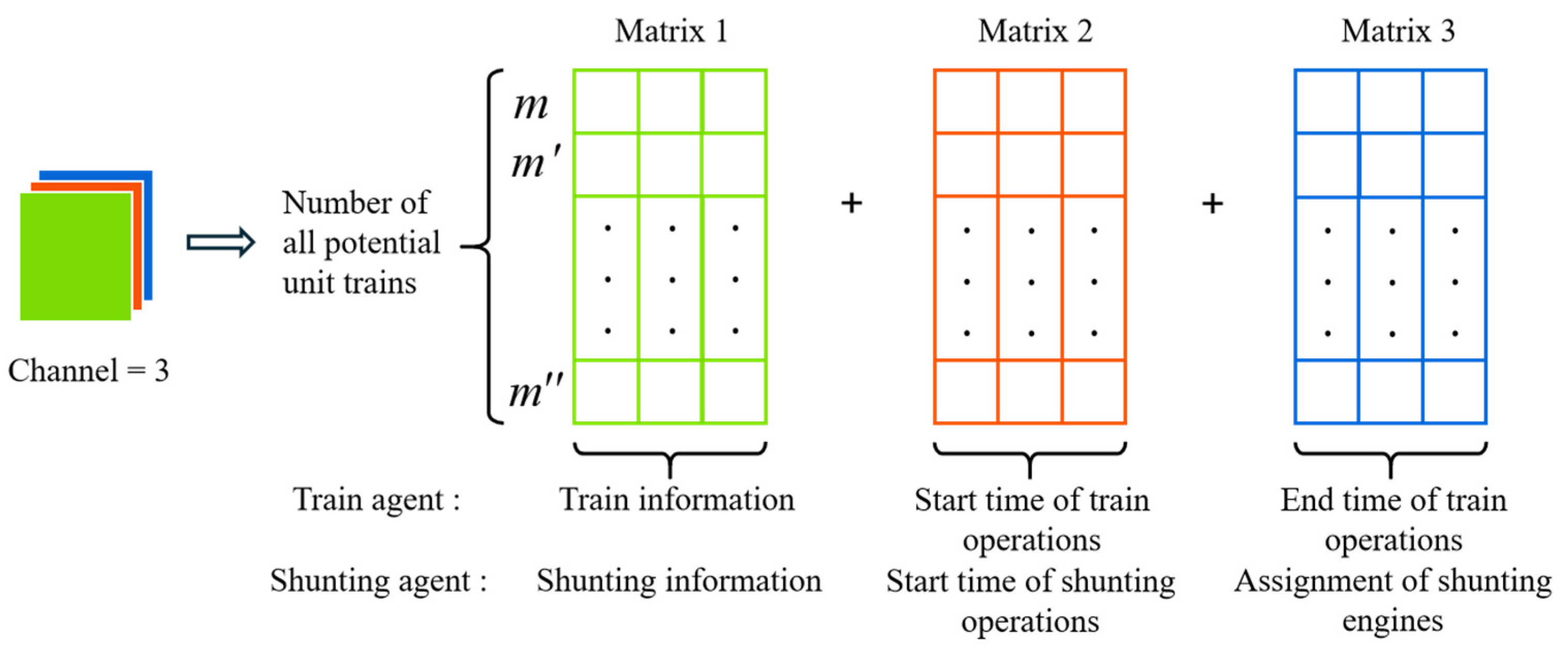
Considering the temporal and spatial dimensions of train movements, the local state of each agent is represented by a three-channel matrix, as depicted in Figure 2. This matrix integrates both static and dynamic information, including scheduling attributes such as operational types and times. The changes in the system’s local state and the station’s operational conditions are described from the perspectives of both the train agent and the shunting agent.
To account for all train splitting plans, the height of each matrix is set to match the number of potential unit trains. For the train agent, each channel includes scheduling features such as train information, and the start and end times of operations. The shunting agent focuses on observing the status of three shunting operations and the current locations of shunting engines. Its local state consists of three matrices: a shunting information matrix, a shunting operations start time matrix, and a shunting engines assignment matrix. All elements in the state matrix are initialized to zero, except for known information.
The two agents acquire their respective local state at each time step t , which are then input into their corresponding CNNs. This architecture design helps the agents to effectively utilize spatiotemporal information and make adaptive decisions in complex and dynamic environments.

4.3. Action Space

By extracting and learning state features, the two agents are required to jointly make decisions for the next step within the action space. This paper proposes a knowledge-based composite scheduling rule set as the action space. This set incorporates splitting plan rules and unloading system capacity distribution strategies into traditional heuristic scheduling, resembling the operational principles of marshaling yards [8], and integrates decision-making concepts aligned with the objective functions. Table 4 presents the scheduling rules for the train agent.
We define the action space in terms of the sequence of operation, train composition, and train type. In train composition scheduling, splitting plans are considered. The first composition rule allocates unit trains based on the unloading capacity to maximize the efficiency of the hybrid unloading system. To simplify calculations, the capacity of the unloading system is related to the number of dumpers F and the unloading time e . Therefore, we can use Equation (27) to compare the capacity of these two unloading systems.
Ω = H 1 H 2 F 1 / e 1 F 2 / e 2
The subscripts 1 and 2 represent the two unloading systems, and   H 1 and H 2 denote the number of unit trains assigned to each respective system. The Ω represents the difference in the ratio of operational quantity to capacity between the two unloading systems. When Ω > 0 , it signifies that unloading system 2 has a higher capacity, making it preferable to select trains corresponding to this system. When Ω < 0 , the situation is exactly the opposite. The train type scheduling rule focuses on comprehending the objective function and the constraints of combination. The combination of the above three types of rules forms the composite action set for the train agent.
The action set for the shunting agent, detailed in Table 5, includes two categories: selecting the shunting engine with the earliest availability to reduce train waiting time, and selecting the nearest engine to minimize running time. These rules focus on optimizing each objective function, and by incorporating regional operations, the action space can adapt to various shunting operation modes, which is consistent with the operational rules in marshaling yards [8].

4.4. Reward Function

When the two agents generate joint actions and interact with the environment, they receive corresponding local rewards that guide their optimization. To achieve Pareto optimality in this bi-objective problem, a reward shaping mechanism incorporates Pareto rewards into local rewards, improving the overall decision-making process [34]. Local rewards focus on each agent’s objectives, while Pareto reward shaping promotes strategic collaboration. In order to illustrate the calculation of rewards, we introduce the symbols shown in Table 6.

4.4.1. Local Reward for the Train Agent

The train agent’s local rewards correspond to the objective function   Z 1   and are divided into two parts: step rewards for each shunting operation and terminal rewards for outbound train combinations. Step rewards update based on the completion times of the three shunting operations in each schedule, calculated using the principle of earliest availability. To illustrate this, the step reward calculation process for the train agent is explained in Algorithm 1, using a unit train m with specific start operation locations p 1 ,   p 5 ,   p 6 as an example.
Algorithm 1 Step rewards for the train agent
Input :   τ i , c i , g i m , e i m , w i m , d i m p , l p * p , t f 1 * , t f 2 * , t k 1 , t k 2 , t k 3 , p k 1 , p k 2 , p k 3
Output :   r t 1 i m t r a i n , r t 2 i m t r a i n , r t 3 i m t r a i n
1 :   for   i ,   m     from   a t t r a i n    do
2:     if 1st shunting operation then
3 :                     Select   the   dumper   f * = arg min f F i m t f 1 ;
4 :                     Calculate   start   shunting   operation   time   by   comparing   earliest   available   time   of   train ,   shunting   engine   and   unloading   track   ζ i m p 1 = max τ i + c i , t k 1 + l p k 1 p 1 , t f 1 * d i m p 1 ;
5 :                     Calculate   start   unloading   time   by   comparing   earliest   available   time   of   train   and   unloading   track   μ i m = max ζ i m p 1 + d i m p 1 , t f 2 * ;
6 :                     Calculate   step   reward   r t 1 i m t r a i n = μ i m + e i m τ i g i m ;
7 :                     Update   t k 1 = ζ i m p 1 + d i m p 1 ,   p k 1 = p 2 ,   t f 1 * = μ i m + e i m ;
8:      end
9:      if 2nd shunting operation then
10 :                   Calculate   start   shunting   operation   time   by   comparing   earliest   available   time   of   train ,   shunting   engine   ζ i m p 5 = max μ i m + e i m , t k 2 + l p k 2 p 5 ;
11 :                   Calculate   step   reward   r t 2 i m t r a i n = ζ i m p 5 + d i m p 5 + w i m μ i m + e i m g i m ;
12 :                   Update   t k 2 = ζ i m p 5 + d i m p 5 ,   p k 2 = p 6 ,   t f 2 * = ζ i m p 5 ;
13:     end
14:     if 3rd shunting operation then
15:          Calculate   start   shunting   operation   time   by   comparing   earliest   available   time   of   train ,   shunting   engine   ζ i m p 6 = max ζ i m p 5 + d i m p 5 + w i m , t k 3 + l p k 3 p 6 ;
16:          Calculate   step   reward   r t 3 i m t r a i n = ζ i m p 6 + d i m p 6 ζ i m p 5 + d i m p 5 + w i m g i m ;
17:          Update   t k 3 = ζ i m p 6 + d i m p 6 ,   p k 3 = p 8 ;
18:     end
19: end
Once all train schedules have been completed, the problem becomes a train combination problem, also known as a static allocation problem with connection time and combination constraints. The terminal reward is calculated using a heuristic algorithm inspired by the greedy approach, which prioritizes maximizing outbound train combinations and employs a forward-looking window strategy to improve global optimization. The detailed calculation process is demonstrated in Algorithm 2.
Algorithm 2 Terminal rewards for the train agent
Input :   η i m , g i m , u i , q c , with the window size = 2, slide step size = 1
Output :   δ i m c , q i m , φ c u , λ c n , r t 4 t r a i n
1 :   for   c C = 1 , 2 , , C 1  do
2:       Calculate   n c 1 , n c 2 , , n c U ;
3:     Update the remaining unassigned trains after calculate combination of outbound train c   with   U types;
4 :           for   n c u n c 1 , n c 2 , , n c U  do
5 :                     Calculate   n c + 1 1 , n c + 1 2 , , n c + 1 U ;
6:                       u u + 1 ;
7:     end
8 :           if   c < C 1  then
9:          Select the combination plan of outbound train c   with   the   maximum   of   n c u * + n c + 1 u *   from   U × U   alternatives ,   φ c u * = 1 ,   λ c n c u * = 1 ;
10:      for unit trains m assigned to outbound train c  do
11 :                             δ i m c = 1   ,   q i m = q c ;
12:      end
13:      Update the remaining unassigned trains after determining combination of outbound train c ,     c c + 1 ;
14:   end
15:    if   c = C 1  then
16:      Select   the   combination   plan   of   outbound   train   c ,   c + 1 with the maximum n c u * + n c + 1 u * *   from   U × U   alternatives ,   φ c u * = 1 ,   λ c n c u * = 1 ,   φ c + 1 u * * = 1 ,   λ c + 1 n c + 1 u * * = 1 ;
17:           for   unit   trains   m , m   assigned   to   outbound   train   c ,   c + 1  do
18:                             δ i m c = 1   ,   q i m = q c   ,   δ i m c + 1 = 1   ,   q i m = q c + 1 ;
19:     end
20:           Calculate   terminal   reward   r t 4 t r a i n = i I m M i η i m q i m ζ i m p 6 + d i m p 6 g i m ;
21:   end
22: end
Equation (28) demonstrates that the total reward accumulated by the train agent during each episode is equivalent to the negative value of the objective function Z 1 , thereby fulfilling the algorithm’s requirements.
R train = i I m M i η i m r t 1 i m t r a i n + r t 2 i m t r a i n + r t 3 i m t r a i n + r t 4 t r a i n = i I m M i η i m μ i m + e i m τ i + ζ i m p 5 + d i m p 5 + w i m μ i m + e i m                                               + ζ i m p 6 + d i m p 6 ζ i m p 5 + d i m p 5 + w i m + q i m ζ i m p 6 + d i m p 6 g i m = i I m M i η i m q i m τ i   g i m = i I m M i c C δ i m c q c τ i   g i m = Z 1

4.4.2. Local Reward for the Shunting Agent

The local rewards for the shunting agent are determined by the change in the running time of light shunting engines after each shunting operation. For example, if shunting engine k is selected at time step t , and its assigned operation complies with the time interval requirements as depicted in Figure 3, then Equation (29) provides the calculation of the step reward.
r t s h u n t i n g = l p 2 p 6 + l p 8 p 1 l p 2 p 1
At the end of scheduling, the cumulative reward   R s h u n t i n g   corresponds to the negative of the running time of light shunting engines. Multiple experiments revealed that using only step rewards resulted in disorganized shunting operations. To address this, a terminal penalty mechanism has been introduced. After completing scheduling, penalties are imposed based on the number of cross-regional shunting operations performed. A reasonable number of cross-regional operations is permitted, but penalties increase with the number of such operations. Experimental comparisons have led to the determination of appropriate values for terminal penalties as shown in Table 7.

4.4.3. Pareto Reward Shaping

The application of Pareto reward shaping aims to encourage the collaboration and selection of Pareto optimal joint actions based on the overall feedback of the system, by modifying their respective rewards. This approach draws on the ideas of the non-dominated sorting and crowding distance calculation methods used for individual evaluation and selection in the non-dominated sorting genetic algorithm II (NSGA-II). By utilizing these two values, we derive the formulation for Pareto reward shaping through the following equations:
r t P a r e t o = 1 rank R t r a i n , R s h u n t i n g + χ crowding_distance R t r a i n , R s h u n t i n g
r t z = r t z + r t P a r e t o 1 + ρ z r t z / r t P a r e t o z train ,   shunting
χ is a weight factor used to balance the importance of crowding distance relative to rank. To align the Pareto reward with the scale of local rewards, ρ t r a i n and ρ s h u n t i n g are calibrated based on the range of local rewards observed during early training episodes.

4.5. Algorithm Framework

In this algorithm, each agent z train , shunting employs an A2C network for state learning and decision-making. During the interaction between the agents and the environment, experience tuples b are stored in a shared experience replay buffer B . Once the replay buffer accumulates a batch size B , it turns into a training process to update the actor network π z o t z , a t z ; θ z and critic network v z s t ; ω z .
The first step is to compute the loss function for the critic network L ω z . To enhance the stability of the training process, a target network v z s t ; ω z with an identical structure to the critic network is employed to compute the target value Y b as follows:
Y b = r b z + γ v z s b + 1 ; ω z
L ω z = 1 2 B b = 1 B v z s b ; ω z Y b 2
The critic network parameters are optimized using the batch gradient descent algorithm with learning rate α z , and the target network’s parameters are smoothly updated using factor σ as follows:
ω z L ω z = 1 B b = 1 B v z s b ; ω z Y b   ω z v z s b ; ω z
ω z = ω z α z   ω z L ω z
ω z = σ ω z + 1 σ ω z
The parameters of the actor network must be updated synchronously to ensure the effective guidance of the agent’s behavior. The policy gradient θ z D θ z and actor network parameter θ z updates are calculated as follows:
θ z D θ z = 1 B b = 1 B Y b v z s b ; ω z   θ z log π z o t z , a t z ; θ z
θ z = θ z + β z   θ z D θ z
The actor network continuously refines its strategy based on the agent’s experiences, enabling better adaptation to the environment and more optimal behavior. Iterative training leads to the convergence of both the actor and critic networks. The interaction and training processes alternate iteratively until the algorithm meets the termination condition. An overview of the algorithm framework is shown in Figure 4.

5. Case Study

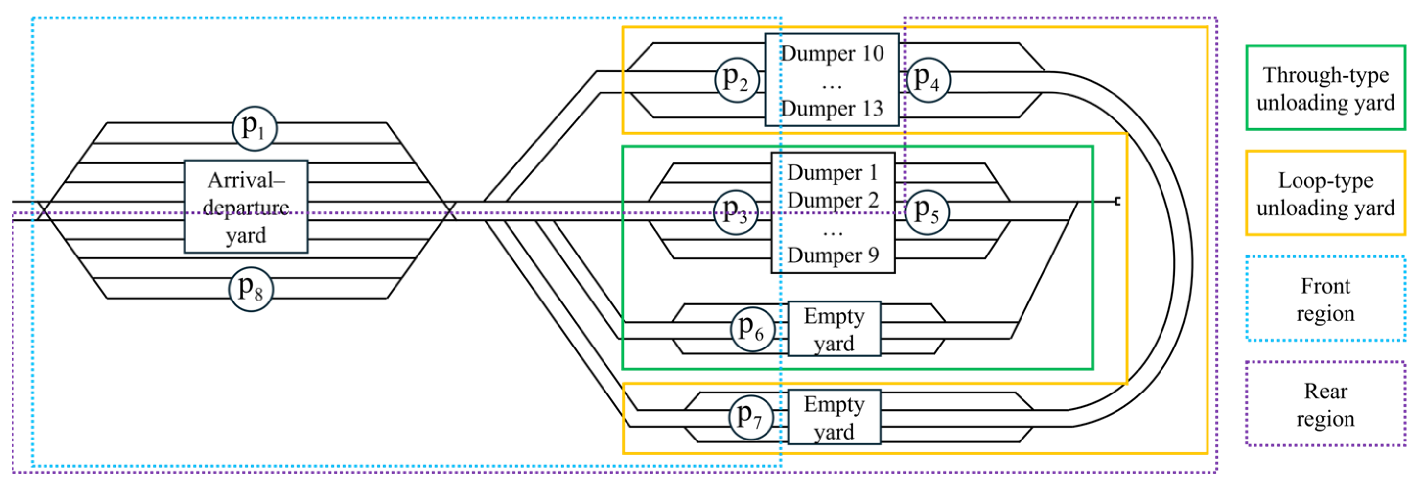
In this section, we demonstrate the effectiveness and applicability of the proposed algorithm by implementing it within the context of the H port station, located at a heavy haul railway in China. As a crucial hub for sea–rail intermodal transport, H port station handles substantial coal unloading and transfer tasks. With the increasing transportation demands and station workloads, the coordination between different operational plans has become more complex. Therefore, the intelligent generation of an integrated operation plan for H port station is essential for improving operation efficiency.

5.1. Background and Parameters

The layout of H port station is shown in Figure 5. The station employs a hybrid unloading system: a through-type system with nine double-dumper sets for unloading 5 kt unit trains (shown in green box), and a loop-type system with four quadruple-dumper sets for unloading 10 kt unit trains (shown in orange box). According to operational time standards, the arrival inspection and splitting time for inbound trains, as well as the combination and departure inspection time for outbound trains, are each 30 min. The unloading time for 5 kt and 10 kt unit trains is 60 min, with coal cleaning times of 20 min and 30 min, respectively. Based on the yard’s scale and operational requirements, the shunting operation times are listed in Table 8.
The station’s three-hour stage plan is the core element guiding its operations. For this study, 14 inbound trains arriving between 10:00 and 13:00 on a specific day were selected as research subjects. Table 9 lists their arrival times, weights, types, and corresponding unit trains, forming a set of 53 candidate unit trains.
Considering operational durations, 13 outbound trains scheduled between 13:40 and 16:40 on the same day were selected. Factoring in routine maintenance tasks for the dumpers and shunting engines, the following configurations are established: seven sets of double-dumpers (f1, f2, f3, f4, f5, f6, and f7) and three sets of quadruple-dumpers (f10, f11, and f12) were available for unloading, along with a total of nine available shunting engines (k1, k2, k3, k4, k5, k6, k7, k8, and k9).
Considering the scale of the problem, extensive experiments were conducted to determine the optimal parameter combination for this problem. The optimal parameters were determined as follows: the total number of episodes was set to 10,000, with the experience buffer size encompassing all steps from 15 complete episodes. The discount factor for target value calculation was 0.99. During experience replay, the Adam optimizer was used, and the learning rates for both actor and critic networks were set to 1 × 10⁻⁴. The target network update parameter was also set to 1 × 10⁻⁴. All computations were performed on a personal computer with an Intel Core i7-11800H 2.3 GHz CPU and 16 GB RAM.

5.2. Results and Analysis

5.2.1. Computational Results

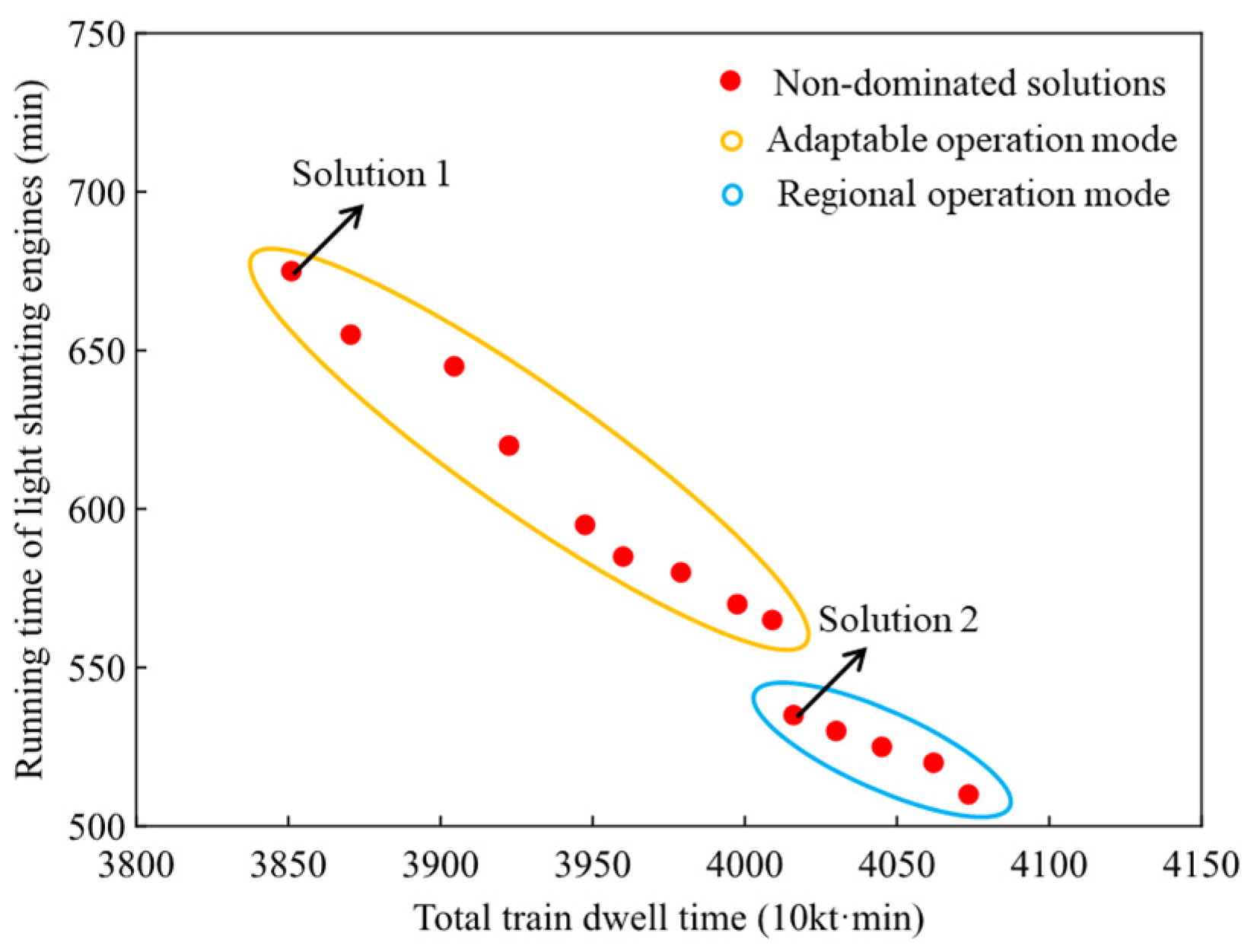
This section analyzes the results of applying the proposed algorithm. Figure 6 shows the Pareto non-dominated set, which is divided into two parts: one corresponding to the adaptable operation mode and the other to the regional operation mode. Comparing the two solution sets, it is evident that the adaptable operation mode minimizes the total train dwell time but increases the running time of light shunting engines due to additional penalties. In contrast, the regional mode results in more stable running routes but increases train dwell time. The widespread distribution of the Pareto front provides decision-makers with flexibility in balancing train dwell time with shunting operation modes.
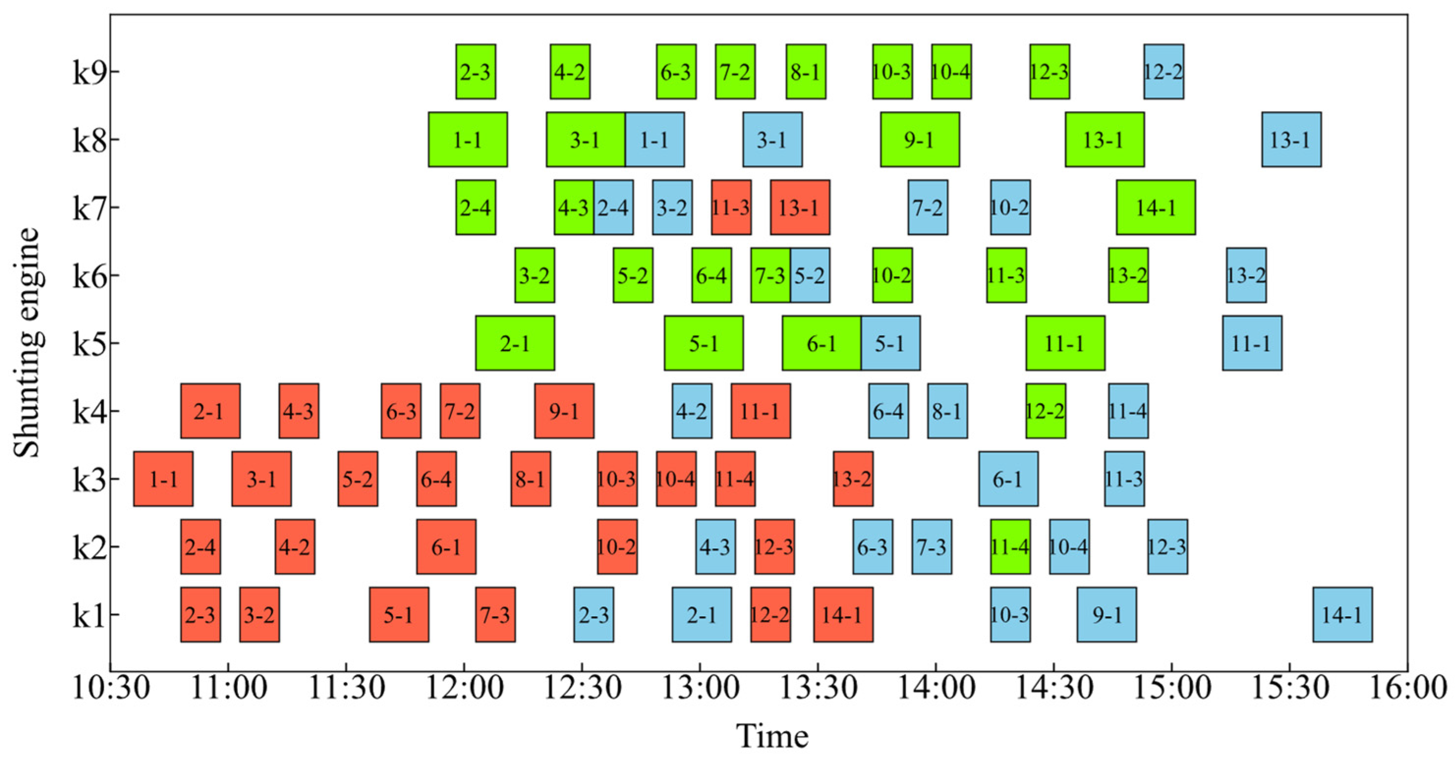
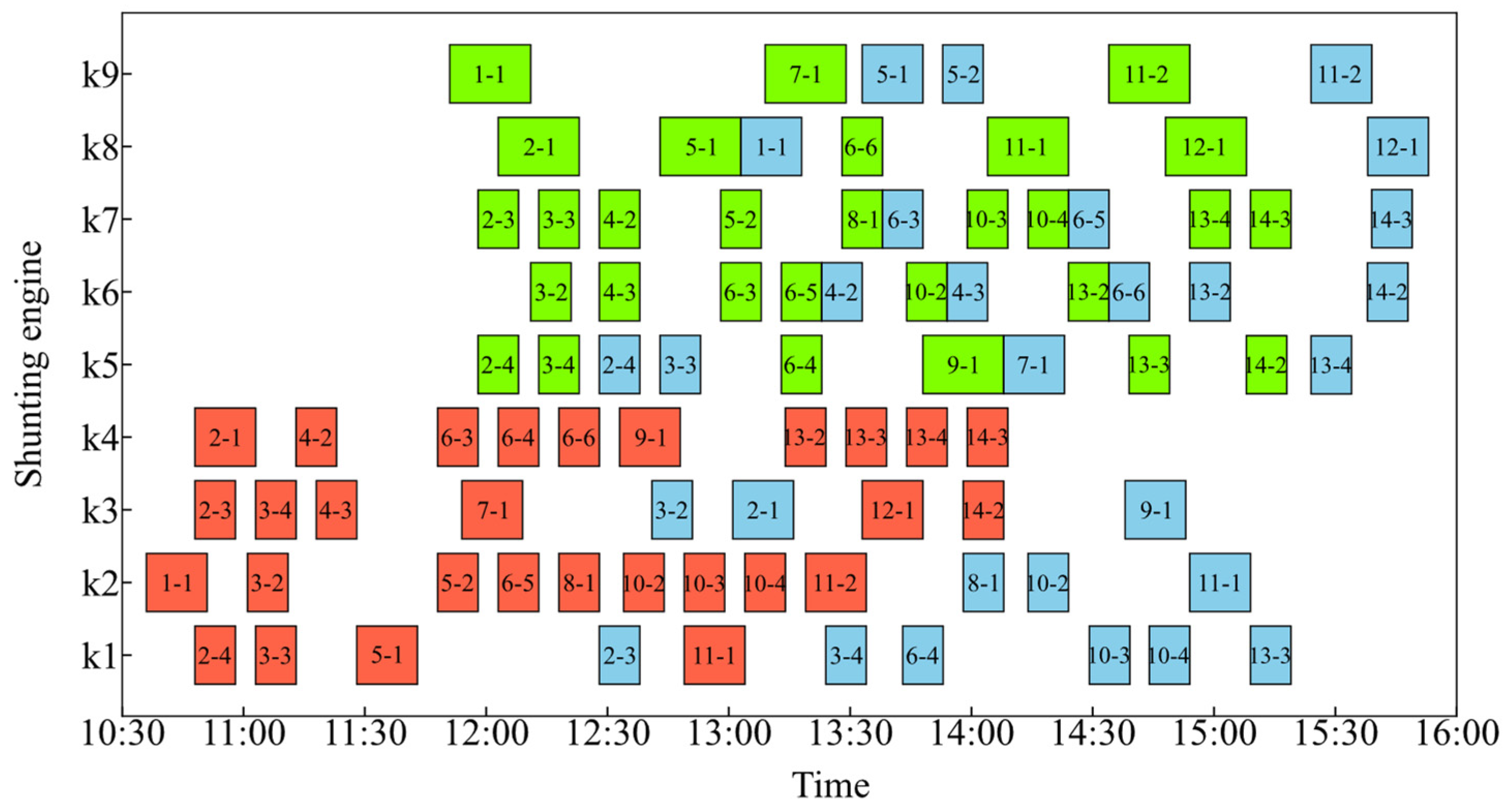
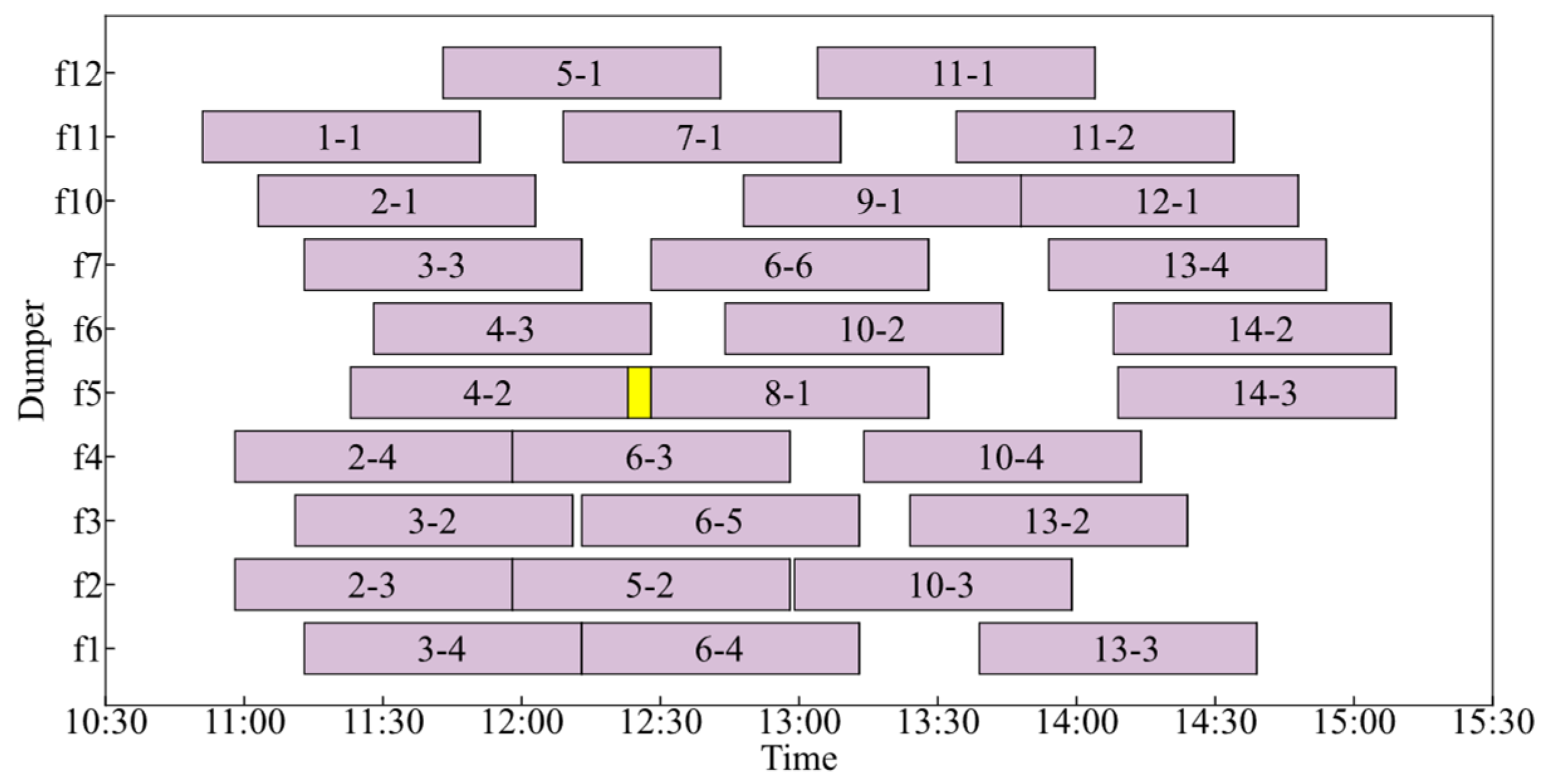
For further analysis, each representative solution of the two parts was selected. The objective values for Solution 1 are 3851 (10 kt·min) and 675 (min), while for Solution 2 they are 4016 (10 kt·min) and 535 (min). Figure 7, Figure 8, Figure 9 and Figure 10 show the Gantt charts for shunting engines and dumpers for both solutions. The charts reflect equipment utilization, with the horizontal axis representing time and the vertical axis indicating equipment. The numbers in the charts denote the unit train numbers. In the Gantt charts of the shunting operations, red, green, and blue represent the first, second, and third shunting operations, respectively. The gaps between consecutive operations of the same shunting engine satisfy the time required for movement between locations.
First of all, from Figure 7 and Figure 8, the splitting plans of the two solutions can be observed. The ratio of 10 kt trains to 5 kt trains in both splitting plans are close to the capacity ratio of the two unloading systems: Ω s o l u t i o n 1 0.045 , Ω s o l u t i o n 2 0.048 , with a difference of less than 5%, indicating an effective workload balance between the systems.
In Solution 1, as shown in Figure 7, the division of shunting engines is as follows: k1, k2, k3, and k4 handle the front region, while k5, k6, k8, and k9 are responsible for the rear region. Specifically, k6 and k9 are fixed in the through-type unloading system, while k5 and k8 are fixed in the loop-type system. Shunting engines k2 and k4 utilize gaps to assist k6 and k9, accelerating empty train shunting. While k7 operates flexibly across the station, particularly when multiple inbound trains arrive in quick succession. Its ability to shift between regions ensures continuous shunting capacity and operational fluidity, balancing workloads between the systems. This flexibility makes k7 a key factor in maintaining operational resilience.
In the regional operation mode, shown in Figure 8, k1, k2, k3, and k4 are assigned to the front region, while k5, k6, k7, k8, and k9 handle the rear region, with no cross-region operations. Moreover, k5, k6, and k7 operate within the through-type system, while k8 and k9 are assigned to the loop-type system, ensuring optimal alignment with system requirements. This clear regional division further specifies their respective roles and reduces the running time of light shunting engines.
Figure 9 and Figure 10 demonstrate that the workload of each dumper is balanced, with minimal idle time between operations, indicating high utilization efficiency. The yellow segments represent periods when trains that have completed unloading occupy tracks but have not been shunted. Only a few instances of track occupation are observed, showing effective collaboration between unloading and shunting, thereby maximizing unloading efficiency.
The combination plan for outbound trains is shown in Table 10. All outbound trains meet the requirements for connection time, train combination, and train type. In Solution 1, an extra outbound train remains, which can be allocated to the next stage. Additionally, the proposed forward-looking strategy optimizes the local combination plan. Taking the combination plans for outbound trains 8 and 9 in Solution 1 as an example, unit trains 9-1, 11-3, and 11-4 meet the connection time requirements for outbound train 8, while unit trains 12-2 and 12-3 meet the requirements for outbound train 9. Although the operation completion time of 9-1 is the earliest, its train type matches that of unit trains 12-2 and 12-3 and meets the requirements for the combination. Therefore, 9-1 is combined with unit trains 12-2 and 12-3 to form outbound train 9. If 9-1 were used as outbound train 8, 11-3, 11-4, 12-2, and 12-3 could not be included in the same outbound train due to inconsistent train types. This demonstrates that the combination algorithm in this paper maximizes the number of cars in adjacent outbound trains while satisfying the combination requirements, resulting in a combination plan that minimizes the total train dwell time.
According to the comprehensive analysis of the two solutions above, we can conclude that both solutions are satisfactory in terms of system resource capability configuration and equipment collaborative scheduling. The collaboration between operations and assignments significantly reduces waiting times and accelerates train movements. The station dispatcher adjusts the specific shunting operation mode flexibly based on the next stage workload and the real-time progress of station operations.

5.2.2. Algorithm Evaluation

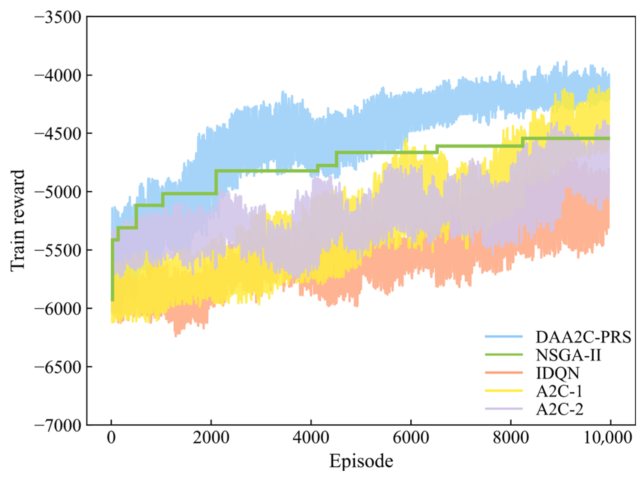
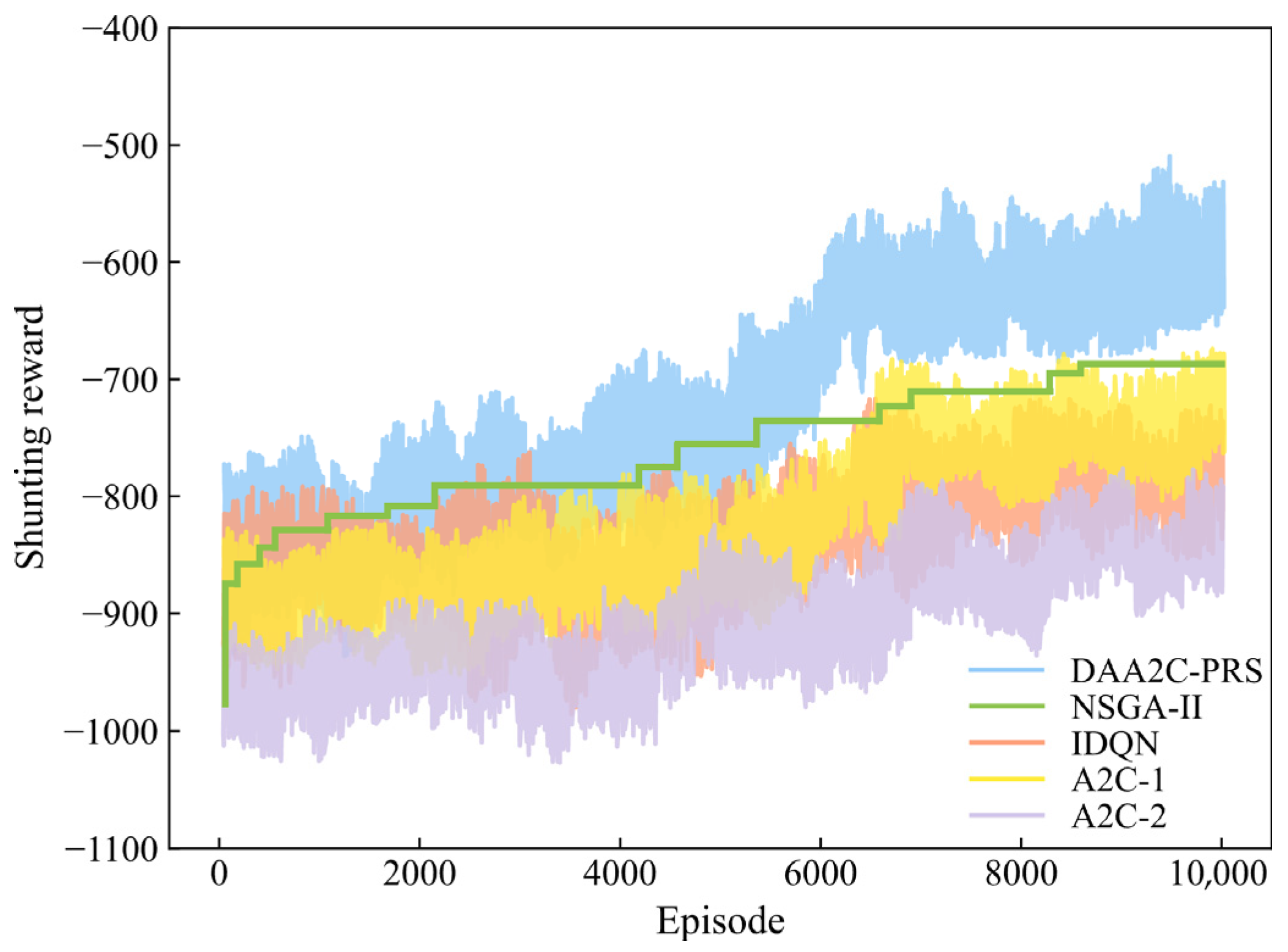
To verify the solution quality and learning efficiency of the proposed algorithm, we conducted a comparative analysis against benchmark methods, including the multi-objective evolutionary algorithm NSGA-II and other DRL methods: independent deep Q-network (IDQN), A2C-1, and A2C-2. IDQN addresses large-scale action spaces by independently estimating Q-values for each action. The A2C-1 and A2C-2 share the foundational framework of our proposed method but differ in their action space design and reward function. Specifically, A2C-1 incorporates a predefined set of 18 heuristic scheduling rules into its action space [35], while A2C-2 excludes the Pareto reward shaping during the training process. These setups are designed to separately explore the impact of knowledge-based scheduling rules and the reward reshaping mechanism on algorithm performance.
The cumulative reward curves for the train and shunting agents during the training process of five algorithms are depicted in Figure 11 and Figure 12, respectively. First of all, our proposed DAA2C-PRS converges to the optimal solution and maintains stability over time. The fluctuations in the trends of the two reward curves are inevitable during the training process, which reflect the exploration process of optimal strategies. Meanwhile, the incorporation of the reward shaping mechanism in DAA2C-PRS plays a pivotal role in mitigating the risk of agents being trapped in local optima and facilitating a balance between the two objective functions. NSGA-II demonstrates certain optimization capabilities but tends to converge prematurely, failing to explore the solution space thoroughly. Furthermore, the slower ascent of the reward curves for A2C-1 compared with DAA2C-PRS indicates the critical importance of action space design in optimizing scheduling strategies. The tailored action space of DAA2C-PRS enables agents to quickly identify promising strategies, thereby minimizing ineffective exploration and enhancing training efficiency.
As training progresses, A2C-2 and IDQN exhibit inferior optimization results, even showing unstable learning behavior. IDQN’s reliance on individual value networks limits the potential for information sharing. On the other hand, A2C-2’s absence of reward shaping and inter-agent communication hampers the development of collaborative strategies, resulting in the incomplete convergence of the reward curve. In contrast, DAA2C-PRS possesses a smooth learning behavior facilitated by the shared experience buffer and reward shaping mechanism, which helps agents to effectively perceive changes in each other’s states and behaviors, leading to dynamic strategy adjustments. Consequently, the agents develop a stable collaborative relationship, which is critical for achieving optimal performance.
To further evaluate the performance of the proposed algorithm on different scale problems, we conducted experiments on three different operation plan horizons (3 h, 6 h, and 12 h) with various numbers of inbound trains. The computational results of these five methods are listed in Table 11, where we selected the solution with the minimum total train dwell time for each result as a representative for comparison.
As the planning horizon expands, the complexity of the scheduling problem significantly increases, with more interactions between agents and a larger decision space to explore. Moreover, the increased number of trains highlights the need for collaboration among trains. In scenarios with a high train density, the efficient utilization of limited resources becomes essential. Without effective collaboration mechanisms, trains may end up competing for the same resources, leading to delays, increased dwell times, and overall inefficiency.
The proposed DAA2C-PRS algorithm demonstrates remarkable superiority and adaptability in addressing these challenges across different scenarios. Its shared experience buffer facilitates information sharing among agents, enabling them to learn from each other’s experiences and adapt their strategies dynamically. The reward shaping mechanism further enhances this by providing agents with a more comprehensive understanding of the long-term consequences of their actions, guiding them towards more efficient and collaborative behavior. This mechanism is vital in environments with a high train density, guiding agents away from local optima and towards globally optimal solutions.
Overall, DAA2C-PRS is able to maintain stable and efficient train scheduling even in environments with a high train density and limited resources, primarily due to its innovative collaborative optimization framework that aligns with the specific characteristics of the scheduling problem.

6. Conclusions

This paper presents an integrated optimization method for heavy haul railway port station operations and formulates an MILP model using a discrete time modeling technique, which incorporates the scheduling of operation plans and equipment resources. To address this complex scheduling problem, we transform it into an MDP and propose a novel DRL approach called DAA2C-PRS. The collaborative behavior of two agents’ interactions with the environment simulates the process of formulating operation plans. State feature representation and the knowledge-based action space are applied to enhance decision-making. Considering that the problem involves a bi-objective approach, a shared experience replay buffer and reward shaping mechanism are introduced to facilitate the information transmission and collaboration between agents, effectively guiding them towards achieving Pareto optimality.
Applying the proposed algorithm to optimize operations at H port station has obtained a set of high-quality Pareto non-dominated solutions. The optimization reveals the alignment of operational workload with resource allocation, achieving a balanced state commensurate with the system’s capabilities. The division of shunting engines is rational under different shunting operation modes, providing flexible scheduling decisions to accommodate real-time operational demands. Furthermore, the results from various scenarios indicate that DAA2C-PRS exhibits superior learning behavior and solution quality in comparison with benchmark methods. The collaborative optimization strategy and framework that conforms to the characteristics of the problem improves convergence performance. This integrated framework fills a gap in existing research, which often separates operation scheduling and resource allocation. Its effectiveness in practical scenarios demonstrates its potential to serve as a reference for optimizing similar heavy haul railway port stations and other transportation hubs, such as container ports and intermodal stations, that face similar integrated operations and resource scheduling challenges, thereby promoting the application of collaborative optimization strategies.
Considering the uncertainties present in real operations, such as weather variations and equipment failures, constructing more flexible and reliable scheduling systems is a vital direction for research. However, the current model has limitations that hinder its ability to fully address these challenges. It assumes a relatively stable operational environment, leaving its performance in handling large-scale sudden disruptions untested. To enhance adaptability and robustness, examining scheduling strategies across different operational contexts is essential. Future work will focus on integrating robust optimization to better handle extreme uncertainties, scaling the algorithm to suit larger stations and exploring transfer learning to improve its adaptability across diverse contexts.

Author Contributions

Conceptualization, Y.W. and S.H.; methodology, Y.W. and S.H.; software, Y.W. and H.T.; validation, Y.W. and Z.L.; formal analysis, H.T.; investigation, S.H.; resources, Y.W.; data curation, Z.L.; writing—original draft preparation, Y.W. and Z.L.; writing—review and editing, Y.W. and S.H.; visualization, H.T.; supervision, S.H.; project administration, Y.W. and S.H.; funding acquisition, S.H. All authors have read and agreed to the published version of the manuscript.

Funding

This research was funded by the Fundamental Research Funds for the Central Universities of Ministry of Education of China (2024JBZX038) and the Research Project of China State Railway Group (N2024X022).

Data Availability Statement

The original contributions presented in this study are included in the article. Further inquiries can be directed to the corresponding author.

Conflicts of Interest

The authors declare no conflicts of interest.

References

  1. Jing, Y.; Zhang, Z. A Study on Car Flow Organization in the Loading End of Heavy Haul Railway Based on Immune Clonal Selection Algorithm. Neural Comput. Appl. 2019, 31, 1455–1465. [Google Scholar] [CrossRef]
  2. Esteso, A.; Peidro, D.; Mula, J.; Diaz-Madronero, M. Reinforcement Learning Applied to Production Planning and Control. Int. J. Prod. Res. 2023, 61, 5772–5789. [Google Scholar] [CrossRef]
  3. Zhou, H.; Zhou, L.; Guo, B.; Bai, Z.; Wang, Z.; Yang, L. A Scheduling Approach for the Combination Scheme and Train Timetable of a Heavy-Haul Railway. Mathematics 2021, 9, 3068. [Google Scholar] [CrossRef]
  4. Wang, D.; Zhao, J.; Peng, Q. Optimizing the Loaded Train Combination Problem at a Heavy-Haul Marshalling Station. Transp. Res. Part E Logist. Transp. Rev. 2022, 162, 102717. [Google Scholar] [CrossRef]
  5. Chen, W.; Zhuo, Q.; Zhang, L. Modeling and Heuristically Solving Group Train Operation Scheduling for Heavy-Haul Railway Transportation. Mathematics 2023, 11, 2489. [Google Scholar] [CrossRef]
  6. Zhuo, Q.; Chen, W.; Yuan, Z. Optimizing Mixed Group Train Operation for Heavy-Haul Railway Transportation: A Case Study in China. Mathematics 2023, 11, 4712. [Google Scholar] [CrossRef]
  7. Tian, A.-Q.; Wang, X.-Y.; Xu, H.; Pan, J.-S.; Snasel, V.; Lv, H.-X. Multi-Objective Optimization Model for Railway Heavy-Haul Traffic: Addressing Carbon Emissions Reduction and Transport Efficiency Improvement. Energy 2024, 294, 130927. [Google Scholar] [CrossRef]
  8. Boysen, N.; Fliedner, M.; Jaehn, F.; Pesch, E. Shunting Yard Operations: Theoretical Aspects and Applications. Eur. J. Oper. Res. 2012, 220, 1–14. [Google Scholar] [CrossRef]
  9. Zhao, J.; Xiang, J.; Peng, Q. Routing and Scheduling of Trains and Engines in a Railway Marshalling Station Yard. Transp. Res. Part C Emerg. Technol. 2024, 167, 104826. [Google Scholar] [CrossRef]
  10. Adlbrecht, J.-A.; Hüttler, B.; Zazgornik, J.; Gronalt, M. The Train Marshalling by a Single Shunting Engine Problem. Transp. Res. Part C Emerg. Technol. 2015, 58, 56–72. [Google Scholar] [CrossRef]
  11. Deleplanque, S.; Hosteins, P.; Pellegrini, P.; Rodriguez, J. Train Management in Freight Shunting Yards: Formalisation and Literature Review. IET Intell. Transp. Syst. 2022, 16, 1286–1305. [Google Scholar] [CrossRef]
  12. Yu, F.; Zhang, C.; Yao, H.; Yang, Y. Coordinated Scheduling Problems for Sustainable Production of Container Terminals: A Literature Review. Ann. Oper. Res. 2024, 332, 1013–1034. [Google Scholar] [CrossRef]
  13. Kizilay, D.; Eliiyi, D.T. A Comprehensive Review of Quay Crane Scheduling, Yard Operations and Integrations Thereof in Container Terminals. Flex. Serv. Manuf. J. 2021, 33, 1–42. [Google Scholar] [CrossRef]
  14. Jonker, T.; Duinkerken, M.B.; Yorke-Smith, N.; de Waal, A.; Negenborn, R.R. Coordinated Optimization of Equipment Operations in a Container Terminal. Flex. Serv. Manuf. J. 2021, 33, 281–311. [Google Scholar] [CrossRef]
  15. Azab, A.; Morita, H. Coordinating Truck Appointments with Container Relocations and Retrievals in Container Terminals under Partial Appointments Information. Transp. Res. Part E Logist. Transp. Rev. 2022, 160, 102673. [Google Scholar] [CrossRef]
  16. Yue, L.-J.; Fan, H.-M.; Fan, H. Blocks Allocation and Handling Equipment Scheduling in Automatic Container Terminals. Transp. Res. Part C-Emerg. Technol. 2023, 153, 104228. [Google Scholar] [CrossRef]
  17. Yang, Y.; Liang, J.; Feng, J. Simulation and Optimization of Automated Guided Vehicle Charging Strategy for U-Shaped Automated Container Terminal Based on Improved Proximal Policy Optimization. Systems 2024, 12, 472. [Google Scholar] [CrossRef]
  18. Liu, C. Iterative Heuristic for Simultaneous Allocations of Berths, Quay Cranes, and Yards under Practical Situations. Transp. Res. Part E Logist. Transp. Rev. 2020, 133, 101814. [Google Scholar] [CrossRef]
  19. Rosca, E.; Rusca, F.; Carlan, V.; Stefanov, O.; Dinu, O.; Rusca, A. Assessing the Influence of Equipment Reliability over the Activity Inside Maritime Container Terminals Through Discrete-Event Simulation. Systems 2025, 13, 213. [Google Scholar] [CrossRef]
  20. Menezes, G.C.; Mateus, G.R.; Ravetti, M.G. A Hierarchical Approach to Solve a Production Planning and Scheduling Problem in Bulk Cargo Terminal. Comput. Ind. Eng. 2016, 97, 1–14. [Google Scholar] [CrossRef]
  21. Unsal, O.; Oguz, C. An Exact Algorithm for Integrated Planning of Operations in Dry Bulk Terminals. Transp. Res. Part E Logist. Transp. Rev. 2019, 126, 103–121. [Google Scholar] [CrossRef]
  22. Kayhan, B.M.; Yildiz, G. Reinforcement Learning Applications to Machine Scheduling Problems: A Comprehensive Literature Review. J. Intell. Manuf. 2023, 34, 905–929. [Google Scholar] [CrossRef]
  23. Yuan, E.; Cheng, S.; Wang, L.; Song, S.; Wu, F. Solving Job Shop Scheduling Problems via Deep Reinforcement Learning. Appl. soft Comput. 2023, 143, 110436. [Google Scholar] [CrossRef]
  24. Lei, K.; Guo, P.; Wang, Y.; Zhang, J.; Meng, X.; Qian, L. Large-Scale Dynamic Scheduling for Flexible Job-Shop With Random Arrivals of New Jobs by Hierarchical Reinforcement Learning. IEEE Trans. Ind. Inform. 2024, 20, 1007–1018. [Google Scholar] [CrossRef]
  25. Luo, S. Dynamic Scheduling for Flexible Job Shop with New Job Insertions by Deep Reinforcement Learning. Appl. Soft Comput. 2020, 91, 106208. [Google Scholar] [CrossRef]
  26. Huang, J.; Huang, S.; Moghaddam, S.K.; Lu, Y.; Wang, G.; Yan, Y.; Shi, X. Deep Reinforcement Learning-Based Dynamic Reconfiguration Planning for Digital Twin-Driven Smart Manufacturing Systems With Reconfigurable Machine Tools. IEEE Trans. Ind. Inform. 2024, 20, 13135–13146. [Google Scholar] [CrossRef]
  27. Liu, C.; Xu, X.; Hu, D. Multiobjective Reinforcement Learning: A Comprehensive Overview. IEEE Trans. Syst. Man Cybern.-Syst. 2015, 45, 385–398. [Google Scholar]
  28. Wang, M.; Zhang, J.; Zhang, P.; Cui, L.; Zhang, G. Independent Double DQN-Based Multi-Agent Reinforcement Learning Approach for Online Two-Stage Hybrid Flow Shop Scheduling with Batch Machines. J. Manuf. Syst. 2022, 65, 694–708. [Google Scholar] [CrossRef]
  29. Lowe, R.; WU, Y.; Tamar, A.; Harb, J.; Abbeel, P.; Mordatch, I. Multi-Agent Actor-Critic for Mixed Cooperative-Competitive Environments. In Proceedings of the Advances in Neural Information Processing Systems, Long Beach, CA, USA, 4–9 December 2017. [Google Scholar]
  30. Wang, Z.; Yang, K.; Li, L.; Lu, Y.; Tao, Y. Traffic Signal Priority Control Based on Shared Experience Multi-Agent Deep Reinforcement Learning. IET Intell. Transp. Syst. 2023, 17, 1363–1379. [Google Scholar] [CrossRef]
  31. Li, W.; Ni, S. Train Timetabling with the General Learning Environment and Multi-Agent Deep Reinforcement Learning. Transp. Res. Part B Methodol. 2022, 157, 230–251. [Google Scholar] [CrossRef]
  32. Ying, C.; Chow, A.H.F.; Nguyen, H.T.M.; Chin, K.-S. Multi-Agent Deep Reinforcement Learning for Adaptive Coordinated Metro Service Operations with Flexible Train Composition. Transp. Res. Part B Methodol. 2022, 161, 36–59. [Google Scholar] [CrossRef]
  33. Rusca, A.; Popa, M.; Rosca, E.; Rosca, M.; Dragu, V.; Rusca, F. Simulation Model for Port Shunting Yards. IOP Conf. Ser. Mater. Sci. Eng. 2016, 145, 082003. [Google Scholar] [CrossRef]
  34. Mannion, P.; Devlin, S.; Mason, K.; Duggan, J.; Howley, E. Policy Invariance under Reward Transformations for Multi-Objective Reinforcement Learning. Neurocomputing 2017, 263, 60–73. [Google Scholar] [CrossRef]
  35. Han, B.-A.; Yang, J.-J. Research on Adaptive Job Shop Scheduling Problems Based on Dueling Double DQN. IEEE Access 2020, 8, 186474–186495. [Google Scholar] [CrossRef]
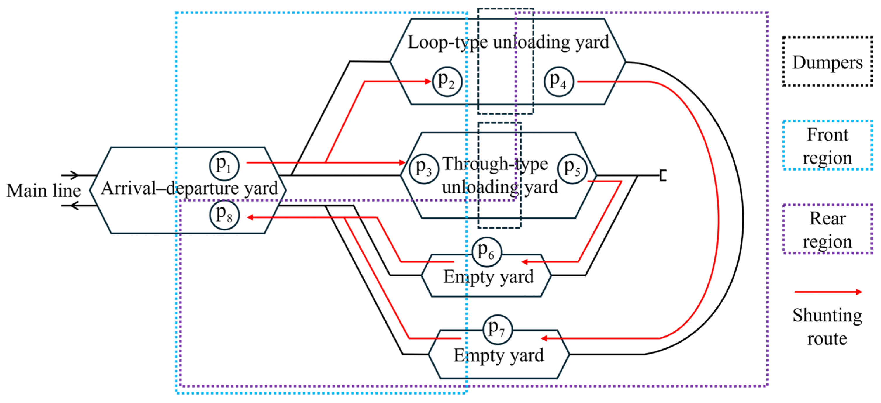
Figure 1. Representative layout of hybrid unloading system.
Systems 13 00762 g001
Figure 2. The local state of the train agent and the shunting agent.
Systems 13 00762 g002
Figure 3. Step reward for the shunting agent.
Systems 13 00762 g003
Figure 4. Overview of the algorithm framework.
Systems 13 00762 g004
Figure 5. Layout of H port station.
Systems 13 00762 g005
Figure 6. Pareto non-dominated set.
Systems 13 00762 g006
Figure 7. Shunting operation Gantt chart of Solution 1. The red, green, and blue segments represent the first, second, and third shunting operations, respectively.
Systems 13 00762 g007
Figure 8. Shunting operation Gantt chart of Solution 2. The red, green, and blue segments represent the first, second, and third shunting operations, respectively.
Systems 13 00762 g008
Figure 9. Dumper Gantt chart of Solution 1. The purple segments represent the unloading operations. The yellow segments represent periods when trains that have completed unloading occupy tracks but have not been shunted.
Systems 13 00762 g009
Figure 10. Dumper Gantt chart of Solution 2. The purple segments represent the unloading operations. The yellow segments represent periods when trains that have completed unloading occupy tracks but have not been shunted.
Systems 13 00762 g010
Figure 11. Training process of train agent.
Systems 13 00762 g011
Figure 12. Training process of shunting agent.
Systems 13 00762 g012
Table 1. Splitting plans of inbound trains.
Weight of Inbound TrainsOptions for Splitting Plans
5 kt(1) 5 kt unit train
10 kt(1) 10 kt unit train
(2) 5 kt unit train + 5 kt unit train
15 kt(1) 10 kt unit train + 5 kt unit train
(2) 5 kt unit train + 5 kt unit train + 5 kt unit train
20 kt(1) 10 kt unit train + 10 kt unit train
(2) 10 kt unit train + 5 kt unit train + 5 kt unit train
(3) 5 kt unit train + 5 kt unit train + 5 kt unit train + 5 kt unit train
Table 2. Definitions of sets, indices, and parameters.
SymbolsDescriptions
I Set   of   inbound   trains ,   indexed   by   i , i , i I .
M i Set of all potential unit trains in inbound train i ,   indexed   by   m , m , m M i .
F i m , f Set of dumpers correspond to unit train m in inbound train i ,   indexed   by   f F i m .
K , k Set   of   shunting   engines ,   indexed   by   k K .
P Set of operation locations, indexed by p , p , p P .
P i m Set of start locations of the shunting operation for unit train m in inbound train i .
p * The end location corresponds to the start location p of the shunting operation.
g i m Weight and formation of unit train m in inbound train i , g i m { 0.5 , 1 } .
t 0 , t 1 The start time and end time of the scheduling period.
t , t , t Index of discretized times within the scheduling period.
τ i Arrival time of inbound train i .
j i Arrival inspection and splitting time of inbound train i .
d i m p Shunting operation time of unit train m in inbound train i at shunting operation location p .
l p * p Running time of shunting engine from the end location p * of last operation to the start location p of the next operation.
e i m Unloading time of unit train m in inbound train i .
w i m Coal cleaning time of unit train m in inbound train i .
C Set of outbound trains, indexed by c C .
q c Departure time of outbound train c .
h c Combination and departure inspection time of outbound train c .
U , u Set of types of railcars, indexed by u U .
u i Type of railcars in inbound train i .
N , n Set of weight and composition of trains, indexed by n { 0 . 5 ,   1 ,   1 . 5 ,   2 } .
n i Composition of inbound train i .
Q A maximum positive constant.
Table 3. Definitions of decision variables.
VariablesDescriptions
η i m Binary variable, 1 if inbound train i split into unit train m , 0 otherwise.
x i m f Binary variable, 1 if unit train m in inbound train i is assigned to dumper f , 0 otherwise.
y k t i m p Binary variable, 1 if unit train m in inbound train i starts shunting operation at location p by shunting engine k at time t , 0 otherwise.
ψ i m p k i m p k Binary variable, 1 if shunting operation at location p by shunting engine k for unit train m in inbound train i   is   the   preceding   operation   of   shunting   operation   at   location   p by shunting engine k for   unit   train   m   in   inbound   train   i , 0 otherwise.
ε i m f i m f Binary variable, 1 if unit train m in inbound train i unloads at dumper f before   unit   train   m   in   inbound   train   i , 0 otherwise.
δ i m c Binary variable, 1 if unit train m in inbound train i is assigned to outbound train c , 0 otherwise.
φ c u Binary variable, 1 if type of railcars in outbound train c is u , 0 otherwise.
λ c n Binary variable, 1 if composition of outbound train c is n , 0 otherwise.
ξ k i m p Nonnegative integer variable, unit train m in inbound train i starts shunting operation time at location p by shunting engine k .
ζ i m p Nonnegative integer variable, unit train m in inbound train i starts shunting operation time at location p .
μ i m Nonnegative integer variable, unit train m in inbound train i starts unloading operation time.
Table 4. Scheduling rules for the train agent.
RulesDescriptions
Sequence 1Select the unit train with the maximum number of remaining shunting operations.
Sequence 2Select the unit train with the minimum number of remaining shunting operations.
Sequence 3Select the unit train that completes unloading operations earliest.
Composition 1Select the unit train composition with greater capacity in the unloading system.
Composition 2Select the unit train composition with relatively idle resources in the unloading system.
Type 1Select the unit train type with the maximum number of types at the station currently.
Type 2Select the unit train type with the same type of outbound trains waiting for departure.
Table 5. Scheduling rules for the shunting agent.
RulesDescriptions
Regional 1Select the shunting engine with the earliest available time in the specific region.
Regional 2Select the shunting engine with the shortest running time to the start location in the specific region.
Cross-regional 1Select the shunting engine with the earliest available time among regions.
Cross-regional 2Select the shunting engine with the shortest running time to the start location among regions.
Table 6. Definitions of symbols in reward calculations.
SymbolsDescriptions
k 1 , k 2 , k 3 The shunting engines corresponding to the 1st, 2nd, and 3rd shunting operations for the unit train are determined by the shunting agent.
t k 1 , t k 2 , t k 3 The   earliest   available   time   of   shunting   engines   k 1 , k 2 , k 3 .
p k 1 , p k 2 , p k 3 The   end   location   of   the   last   operation   of   shunting   engines   k 1 , k 2 , k 3 .
f * The selected dumper.
t f 1 , t f 2 The earliest available time of unloading track in front of and behind the dumper f .
r t 1 i m t r a i n , r t 2 i m t r a i n , r t 3 i m t r a i n The step rewards obtained by the train agent for the 1st, 2nd, and 3rd operations of unit train m .
n c u Maximum combination of outbound train c with type u .
u c Type of outbound train c .
q i m Departure time of unit train m .
n * , n * * The   selected   combinations   of   outbound   train   c , c + 1 .
u * , u * * The   selected   types   of   outbound   train   c , c + 1 .
r t 4 t r a i n The terminal reward of the train agent.
r t s h u n t i n g The step rewards obtained by the shunting agent.
r t P a r e t o Pareto reward.
χ Weight factor.
ρ t r a i n Scaling factor of the train agent.
ρ s h u n t i n g Scaling factor of the shunting agent.
G Number of cross-regional operations.
R t r a i n The cumulative reward of the train agent.
R s h u n t i n g The cumulative reward of the shunting agent.
Table 7. Terminal penalty for the shunting agent.
Number of Cross-Regional OperationsTerminal Penalty
G 0 , 1 , 2 , 3 , 4 , 5 30 × G
G 6 , 7 , 8 , 9 , 10 50 × G
Other 100 × G
Table 8. Shunting operation times.
Shunting OperationOperation Time (min)
5 kt Unit Train10 kt Unit Train
Arrival yard to unloading yard 10   ( p 1 p 3 ) 15   ( p 1 p 2 )
Unloading yard to empty yard 10   ( p 5 p 6 ) 20   ( p 4 p 7 )
Empty yard to departure yard 10   ( p 6 p 8 ) 15   ( p 7 p 8 )
Table 9. Inbound trains information.
No.Inbound Train NumberArrival TimeWeightTypeCandidate Set of Unit Train
10 kt5 kt
116,16510:0610 ktC641-11-2, 1-3
228,05310:1820 ktC802-1, 2-22-3, 2-4, 2-5, 2-6
316,74910:2915 ktC703-13-2, 3-3, 3-4
415,68310:4210 ktC644-14-2, 4-3
516,82710:5815 ktC805-15-2, 5-3, 5-4
627,14111:0920 ktC706-1, 6-26-3, 6-4, 6-5, 6-6
716,17711:2410 ktC647-17-2, 7-3
8650311:345 ktC64-8-1
915,72911:4810 ktC709-19-2, 9-3
1016,84512:0415 ktC8010-110-2, 10-3, 10-4
1128,10312:1920 ktC8011-1, 11-211-3, 11-4, 11-5, 11-6
1215,74112:3110 ktC7012-112-2, 12-3
1316,86712:4415 ktC8013-113-2, 13-3, 13-4
1415,77912:5910 ktC7014-114-2, 14-3
Table 10. Combination plans of two solutions.
No.Departure TimeSolution 1Solution 2
TypeFormationCombinationTypeFormationCombination
113:40C6020 kt1-1, 4-2, 4-3C7010 kt3-2, 3-3
213:55C8020 kt2-1, 2-3, 2-4C8020 kt2-1, 2-3, 2-4
314:08C7015 kt3-1, 3-2C6015 kt1-1, 4-2
414:27C8015 kt5-1, 5-2C7015 kt3-4, 6-3, 6-4
514:42C6015 kt7-2, 7-3, 8-1C8015 kt5-1, 5-2
614:56C7020 kt6-1, 6-3, 6-4C6020 kt4-3, 7-1, 8-1
715:12C8015 kt10-2, 10-3, 10-4C8010 kt10-2, 10-3
815:29C8010 kt11-3, 11-4C7020 kt6-5, 6-6, 9-1
915:43C7020 kt9-1, 12-2, 12-3C8020 kt10-4, 11-1, 13-2
1016:04C8015 kt11-1, 13-2C8010 kt13-3, 13-4
1116:14C8010 kt13-1C8010 kt11-2
1216:22C7010 kt14-1C7010 kt14-2, 14-3
1316:34---C7010 kt12-1
Table 11. Performance comparison for five algorithms on different scale problems.
HorizonsNumbers of Inbound Trains ( Z 1   10   kt · min ;   Z 2 min)
DAA2C-PRSNSGA-IIIDQNA2C-1A2C-2
3 h13(3690.5; 580)(3925; 610)(3904; 610)(3841.5; 585)(3836; 600)
14(3851; 675)(4562.5; 690)(4636; 760)(4092.5; 725)(4394; 835)
15(4076; 695)(4503; 720)(4727.5; 805)(4568; 735)(4610.5; 840)
6 h26(7621; 1285)(7910.5; 1360)(7828; 1390)(7885.5; 1395)(7846; 1395)
28(7964; 1400)(8406.5; 1520)(8640.5; 1605)(8587.5; 1630)(8651.5; 1705)
30(8430.5; 1615)(8991.5; 1805)(9289; 1755)(9276; 1790)(9195; 1840)
12 h52(15,943; 2615)(16,775; 2885)(16,796.5; 2905)(16,642; 2890)(16,581; 2920)
56(16,789.5; 2955)(17,542.5; 3105)(17,602; 3220)(17,324; 3215)(17,751.5; 3195)
60(18,196.5; 3140)(19,268; 3305)(19,317.5; 3375)(19,244.5; 3365)(19,405; 3410)
Disclaimer/Publisher’s Note: The statements, opinions and data contained in all publications are solely those of the individual author(s) and contributor(s) and not of MDPI and/or the editor(s). MDPI and/or the editor(s) disclaim responsibility for any injury to people or property resulting from any ideas, methods, instructions or products referred to in the content.