Abstract
Global supply chains often face uncertainties in production lead times, fluctuating exchange rates, and varying tariff regulations, all of which can significantly impact total profit. To address these challenges, this study formulates a multi-country supply chain problem as a Semi-Markov Decision Process (SMDP), integrating both currency variability and tariff levels. Using a Q-learning-based method (SMART), we explore three scenarios: (1) wide currency gaps under a uniform tariff, (2) narrowed currency gaps encouraging more local sourcing, and (3) distinct tariff structures that highlight how varying duties can reshape global fulfillment decisions. Beyond these baselines we analyze uncertainty-extended variants and targeted sensitivities (quantity discounts, tariff escalation, and the joint influence of inventory holding costs and tariff costs). Simulation results, accompanied by policy heatmaps and performance metrics, illustrate how small or large shifts in exchange rates and tariffs can alter sourcing strategies, transportation modes, and inventory management. A Deep Q-Network (DQN) is also applied to validate the Q-learning policy, demonstrating alignment with a more advanced neural model for moderate-scale problems. These findings underscore the adaptability of reinforcement learning in guiding practitioners and policymakers, especially under rapidly changing trade environments where exchange rate volatility and incremental tariff changes demand robust, data-driven decision-making.
1. Introduction
Managing multi-country production systems involves dealing with random production times, transportation times, uncertain exchange rates, and tariff costs. A typical approach is to formulate a Semi-Markov Decision Process (SMDP) [1,2] and solve it under the average reward criterion. Pontrandolfo et al. [3] demonstrated how a reinforcement learning (RL) technique can be applied to a GSCM context. Early studies further emphasized the strategic importance of integrating distributed supply chain activities under global conditions, with a particular focus on tariffs and currency gaps [3,4].
In this study, we build on the global supply chain management (GSCM) framework proposed by Pontrandolfo et al. [3], which employed an RL technique within an SMDP context to coordinate production, distribution, and sourcing across multiple countries. Our primary objective is to investigate how shifts in exchange rates and tariff policies influence both overall profitability and the allocation of orders among various production and distribution options. Leveraging an average-reward SMART learning framework that is cross-validated with a Deep Q-Network, we combine a baseline-versus-uncertainty scenario exploration with targeted sensitivity tests on quantity discounts, tariff escalation, and the joint influence of inventory holding costs and duties; our core contribution is to quantify—under realistic parameters and in light of prior studies—how tariffs in the 25–30% range interact with exchange rate movements to establish a practical ceiling beyond which cross-border procurement rarely remains economically attractive.
To achieve this, we consider a three-country GSCM setting, where each country exhibits distinct exchange rate behavior modeled through random distributions, and shipping options include both within-country and cross-border modes (the latter featuring slow or fast transit choices). We assign typical cost parameters reflecting production expenses, pipeline and inventory costs, and a late delivery penalty if total lead times exceed a threshold. Additionally, when goods cross national borders, a tariff is imposed to capture international trade costs. Both production and transportation lead times follow probability distributions, reflecting real-world variability in manufacturing and logistics processes.
Within this broad setup, we define three main scenarios to systematically explore the impact of altering currency and tariff conditions. In the first scenario, we closely match the conditions and parameter settings originally proposed by Pontrandolfo et al. [3], effectively replicating their base case. Next, we narrow the currency gaps among countries to see how more closely aligned exchange rates affect sourcing strategies. Finally, we vary tariff structures so that each country has a different duty rate, revealing how policy interventions can drive substantial changes in global supply chain decisions. Through these scenarios, we highlight how small or large policy levers—such as incremental tariff adjustments or exchange rate shocks—lead to different strategies in production location, shipping mode selection, and inventory management. In doing so, we aim to offer insights for both practitioners (facing rapidly evolving trade conditions) and policymakers (examining broader effects of tariff changes).
Following the spirit of Pontrandolfo et al. [3], we model customer-demand arrivals in each country as an Erlang (Gamma) process with shape and scale (medium variability, CV ); the uncertainty-extended scenarios re-run the model under (heavy-tailed, CV ) and (light-tailed, CV ) to stress test policy robustness against demand variance. Unlike the original study—which compared local heuristics (LH, BH) and an RL-based SMART policy under multiple uncertainty levels—we focus exclusively on a Q-learning-based (SMART) SMDP in our core experiments. At the same time, to validate the model and confirm that the learned policy aligns with a more advanced, neural network approach, we also implement a Deep Q-Network (DQN). The DQN is thus deployed primarily as a verification step, showing that the tabular RL outcomes remain robust under a known problem size, one widely used in the literature to capture tariff effects. Consequently, while DQN results corroborate the viability of our Q-learning solution, we continue with Q-learning for the main analyses in order to more clearly illustrate how tariff variations impact the near-optimal sourcing and shipping decisions.
2. Literature Review
2.1. Reinforcement Learning for Logistics Optimization
Efforts to operationalize learning algorithms for supply chain optimization have been extensive. Researchers indicate that reinforcement learning can facilitate coordination in competitive supply chains, yet achieving convergence to truly optimal policies across distributed settings remains challenging [5]. A reinforcement learning-based model was applied to the beer game to improve coordination and reduce inventory costs across supply chain members, showing significant performance advantages over traditional ordering policies [6]. Multi-agent reinforcement learning has been applied to supply chain coordination problems. Zhao and Sun [7] developed a coordination framework for multi-agent systems, focusing on improving supply chain decision-making through real-time learning. Puskás et al. (2020) applied reinforcement learning to optimize vehicle platoon coordination in a physical internet-based supply chain, demonstrating cost-efficient logistics through dynamic reconfiguration [8]. A comprehensive survey by Rolf et al. [9] reviewed RL in supply chain management (SCM) and underscored the gap between research prototypes and industrial-scale implementations. Zou et al. [10] further extended logistics-oriented RL by integrating a graph-attention network into a deep RL framework that jointly minimized carbon taxes, cooling costs, and travel distance for fresh food distribution under tight delivery windows, demonstrating the sustainability potential of DRL-based routing. Liu [11] developed a reinforcement learning-based model to optimize coordination and negotiation in cross-border e-commerce supply chains, improving efficiency and reducing decision time.
Recent work further highlights how pricing, financing, and inventory decisions interact under uncertainty. Li and Zheng [12] analyzed an online dynamic pricing problem with unknown, information-driven demand, proving tight revenue bounds relative to clairvoyant and deterministic benchmarks. Complementing that stream, Gurkan et al. [13] showed that a static replenishment pricing policy can rival the profit-optimal dynamic rule when demand variability is moderate. Capital constraints add another layer of complexity: Li and Li [14] designed a revenue-sharing and buy back (RSBB) contract that coordinates a cash-strapped new-energy-vehicle supply chain, with the revenue share decreasing in the retailer’s acceptable bankruptcy risk, whereas the buy back price moves in the opposite direction. Beyond single-product settings, Bergemann et al. [15] characterized the welfare frontier of third-degree price discrimination, establishing that any surplus split between consumers and a monopolist is attainable within well-defined bounds. Finally, industry-specific studies such as that by Gomes et al. [16] demonstrate how tailored scheduling models (e.g., for fabric dyeing) can reduce inventories and set-up times, reinforcing the managerial value of jointly optimizing operational and pricing levers.
2.2. Reinforcement Learning for Inventory Management and Supply Chain Security
Beyond mainstream production and distribution concerns, specialized domains within supply chains have also benefited from RL. Lu and Wu [17] applied multi-agent reinforcement learning to optimize logistics information systems, focusing on improving stability, security, and decision efficiency in supply chain data processing. Kavididevi et al. (2024) [18] utilized IoT-integrated reinforcement learning to enhance the efficiency and reliability of refrigerated transport in cold chain logistics, enabling real-time environmental monitoring and dynamic decision-making to reduce spoilage and energy use. Zhou et al. [19] highlight RL’s capacity to address volatile supply and demand, demonstrating how policy iterations outperform traditional methods in uncertain inventory settings. Liu et al. [20] applied a deep reinforcement learning approach to multi-echelon inventory management, showing that multi-agent learning architectures can effectively reduce total costs and respond dynamically to demand fluctuations. Meanwhile, Aboutorab et al. [21] integrated natural language processing with RL to proactively uncover and mitigate global supply chain disruptions, underscoring the importance of automated, data-driven resilience strategies. Focusing on a capital-intensive domain, Ma et al. [22] proposed a hierarchical RL framework for upstream crude oil scheduling, revealing superior performance relative to conventional operation research techniques in reducing penalties and transportation costs under dynamic supply–demand conditions. Complementing these efforts, Piao et al. [23] formulated a civil aircraft spares network as a partially observable MDP and achieved a 45% efficiency gain via dual-policy multi-agent RL, while Ma et al. [24] coupled Soft Actor–Critic with a blockchain-based zero-trust architecture to optimize inventory under demand uncertainty and ensure tamper-proof traceability. Collectively, these studies illustrate how RL—especially when coupled with domain-specific heuristics, hierarchical structures, or real-time analytics—can flexibly adapt to operational complexities, yielding robust decision-making tools even under high degrees of uncertainty and scale.
2.3. Deep RL and Multi-Agent/Process Control Applications
Reinforcement learning has also seen significant advances through Deep Q-Networks (DQN), introduced initially by Mnih et al. [25], wherein a neural network function approximator replaced the traditional Q-table. Subsequent studies have extended DQN to handle more advanced RL challenges; for instance, Wang and Wang [26] applied it in international logistics for dynamic decision-making under uncertainty, while Double DQN [27], Dueling DQN [28], and Prioritized Experience Replay [29] have further improved stability and performance. Zhu et al. [30] provided a comprehensive survey on transfer learning within deep reinforcement learning, showing how knowledge from external tasks can accelerate learning when faced with new or complex scenarios. Padhye and Lakshmanan [31] focused on a ranking problem and proposed an actor–critic framework that utilizes deep networks to handle large action spaces (i.e., extensive item sets) and reduce variance via advanced policy-gradient techniques. Complementing these algorithmic advances is the safety-critical perspective highlighted by Norouzi et al. [32], who investigated “safe” deep reinforcement learning to manage diesel engine emissions. Their work incorporated a safety filter to enforce output constraints during training, thus reducing the risk of unacceptable solutions. Collectively, these studies underscore the growing sophistication of deep reinforcement learning approaches, whether through improved transfer-learning mechanisms, better handling of large-scale ranking tasks, or embedding explicit safety filters for real-world control systems. In this work, we primarily build our solution using a Q-learning-based SMDP framework; however, we also employ DQN as a secondary method to validate the outcomes of our Q-table approach. By comparing the two, we demonstrate that the Q-learning model’s decisions and results are consistent with and, in some scenarios, closely matched by a deep RL alternative, thus reinforcing confidence in the proposed tabular solution under the given problem constraints.
2.4. Broader Cyber-Physical and Data-Centric Applications of Deep Reinforcement Learning
Recent studies have illustrated the growing applicability of reinforcement learning (RL) in diverse, real-world domains. In mobile robotics, for example, DRL-based solutions have significantly enhanced autonomous navigation strategies and sensor integration, leading to more flexible, self-controlled robots under dynamic conditions [33]. Within sports analytics, offline RL approaches can now leverage large-scale event and tracking data to predict in-game outcomes or optimal decisions, outperforming traditional methods in both accuracy and efficiency [34]. Medical interventions, such as cardiovascular guidewire navigation, benefit from zero-shot RL techniques that generalize to unseen vascular anatomies without retraining [35]. Meanwhile, the financial sector has adopted RL frameworks to handle the challenges of dynamic datasets and market variability, enabling more robust and data-centric trading strategies [36]. Yu et al. [37] extended DQN and DDPG to dynamic edge-computing off-loading for fault diagnosis, showcasing DRL’s ability to orchestrate resource allocation across distributed cyber-physical nodes. These examples underscore RL’s versatility and its ongoing expansion into areas requiring adaptive, data-driven decision-making.
2.5. Research Gap
Taken together, this body of work highlights a rapidly enlarging frontier in which reinforcement learning—spanning both tabular and deep variants—consistently improves coordination, adaptability, and overall performance across an ever-broader array of operational settings. The same versatility positions RL as a particularly promising tool for tariff-sensitive global supply chains that must cope with compounded uncertainties such as currency shocks, shifting trade policies, and environmental pressures; by learning adaptively and scaling to higher complexities, RL frameworks can deliver robust, data-driven policies in precisely these volatile contexts. To the best of our knowledge, despite the breadth of applications reviewed, no prior study simultaneously integrated exchange rate volatility, heterogeneous tariff regimes, and variable decision intervals within a semi-Markov RL framework validated by both tabular and deep methods. The present study fills this gap by applying average-reward SMART learning and validating the resulting policy against a Deep Q-Network in a tariff-sensitive global sourcing setting. Furthermore, we embed the proposed SMART–DQN framework in a two-tier experimental program that extends well beyond static parameter settings. First, a baseline vs. uncertainty-extended scenario exploration introduces demand surges and random transport disruptions to test policy robustness under operational noise. Second, a suite of sensitivity analyses—spanning quantity discounts, systematic tariff escalation, and the joint inventory holding–tariff cost trade-off—demonstrate that the 25–30% tariff band consistently emerges as the tipping point at which cross-border sourcing loses its economic appeal. These layers of validation strengthen the methodological novelty of our study and confirm the managerial relevance of the identified policy threshold.
3. Methodology
In this section, we first formulate the Semi-Markov Decision Process (SMDP) model tailored to global supply chain management (GSCM) problems. We then describe the reinforcement learning (RL) approach, focusing on the SMART algorithm (a Q-learning-based method) to obtain near-optimal solutions under variable transition times. Finally, we introduce Deep Q-Networks (DQNs) as a powerful extension for dealing with larger or more complex state spaces. Although our core experiments relied on a tabular Q-learning approach, we employed DQN primarily as a validation tool, confirming that the policy learned by the SMART algorithm aligns well with results from a deep neural network function approximator in moderate-scale scenarios.
All experiments were executed on the same personal computer (Intel® Core™ i5-6200U @ 2.30 GHz, 8 GB RAM) running Microsoft Windows 10 Pro (22H2). The computational environment comprised Python 3.10.18, JupyterLab 4.3.4, NumPy 1.26.4, SimPy 4.1.1, and Matplotlib 3.10.3.
3.1. Semi-Markov Decision Processes (SMDP)
A Semi-Markov Decision Process (SMDP) is defined by a state space S, an action set A, transition probabilities, rewards, and random transition times. Unlike a standard Markov Decision Process (MDP) that operates in fixed time steps, an SMDP allows variable intervals between decisions. Let be a Markov renewal process, where denotes the state of the system at the m-th decision epoch and is the time of the m-th epoch. The defining property of the SMDP is expressed as
where t represents the random duration until the next decision epoch. In this framework, a policy is a rule prescribing which action to choose when the system is in a particular state . The goal is typically to optimize a performance criterion—commonly the long-run average reward in semi-Markov settings—by selecting the actions that maximize the expected return over time, given the variable transition intervals.
In other words, while (1) shows how the evolution of states and times satisfies the semi-Markov (memoryless) property, the policy indicates the action to be taken once the system enters state s. Although the variable time intervals do not explicitly appear in the notation for , they are inherently accounted for in the process dynamics via the random variable t, as well as in the resulting long-run objective function (e.g., average reward) under time-varying transitions.
3.2. Reinforcement Learning (RL)
Reinforcement Learning (RL) offers a model-freeframework for solving SMDPs by forgoing explicit transition probabilities and instead learning policies through trial-and-error interaction with the environment [2]. Concretely, an RL agent observes states s, selects actions a, and receives rewards r over many episodes. As it gathers experience, the agent refines its action-value function —the estimated long-term value of choosing action a in state s—toward the optimal .
During learning, the agent balances exploration (trying actions that are uncertain) with exploitation (selecting high-value actions found so far). As more transitions are sampled, converges to accurate value estimates, guiding the agent to near-optimal decisions under varying state transitions and rewards. This model-free property is especially advantageous in SMDPs with uncertain or complex dynamics since it dispenses with having to pre-specify detailed transition probabilities or reward structures.
3.3. Smart Algorithm (Average Reward Q-Learning)
In this study, we employed a value iteration-based RL variant for average reward SMDPs, often referred to as the SMART (Semi-Markov Average Reward Technique) algorithm. Unlike discount-based Q-learning, which optimizes the discounted sum of rewards, average reward Q-learning focuses on maximizing , the long-run average reward. The general update rule is
where
- is the learning rate,
- r is the immediate reward received after taking action a in state s,
- is the current estimate of the average reward,
- t is the elapsed time for the transition,
- is the next state, and
- b iterates over all possible actions from .
This update is repeated until convergence, at which point approximates the maximum achievable average reward and the policy is nearly optimal.
3.4. Deep Q-Networks (DQNs)
Deep Q-Networks (DQNs) were first introduced by Mnih et al. [25] as a powerful extension of classical Q-learning, enabling reinforcement learning (RL) to scale to larger or more complex state spaces via deep neural network function approximation. In their pioneering work, the authors demonstrated that a convolutional neural network (CNN) trained end-to-end could learn effective policies from raw images in Atari 2600 games, surpassing many previous hand-engineered approaches. This breakthrough showed that combining standard Q-learning updates [38] with deep function approximators could achieve human-level (and sometimes super-human) performance in high-dimensional tasks.
DQN builds on tabular Q-learning by introducing three main concepts:
- Neural Network Function Approximation: A deep neural network , parameterized by weights , approximates the action-value function . This approach avoids the exponential growth of a tabular Q-learning when the state space becomes large or continuous.
- Experience Replay: Transition tuples collected from the environment are stored in a replay buffer. During training, mini-batches are sampled randomly from this buffer, breaking the strong correlations often present in sequential data and improving the stability of training.
- Target Networks: DQN maintains a separate set of network parameters for the target Q function, which is updated more slowly (e.g., every fixed number of steps) to reduce oscillations and divergence in learning.
In small to medium-sized problems, DQN often achieves good results quickly without requiring exhaustive enumeration of all states, making it especially suitable for preliminary or proof-of-concept experiments in RL-based supply chain models. As problem dimensions increase (e.g., due to larger stock level ranges, additional countries, or more complex dynamics), DQN’s capacity for function approximation becomes even more critical, allowing it to generalize where a tabular Q table would become intractably large.
3.5. Implementation Outline
A high-level summary of the SMART-based procedure applied to this GSCM model is as follows:
- Initialize: Set to some initial value for all states s and actions a. Initialize , the average reward estimate, to 0 or a small number.
- Observe State: Determine the current system state .
- Action Selection: Choose an action a (e.g., shipping mode) using an -greedy or softmax policy based on the current Q-values.
- Simulate: Generate a random production time and shipping time, apply the chosen action, and calculate the realized reward r.
- Update: Compute the transition time t. Update using (2). Periodically adjust via , where is a small step size.
- Transition: Observe the next state . Repeat until convergence or until a predefined number of iterations.
Once the algorithm converges, the resulting Q-table (or function) captures the near-optimal policy dictating how orders should be allocated among shipping modes and production locations. In the following sections, we apply this methodology to three main scenarios differing in exchange rate distributions and tariff structures.
3.6. Modeling Assumptions
The SMART-based simulation rests on the following assumptions, which match or extend the settings used by Pontrandolfo et al. [3] and enable tractable average-reward learning:
- Exchange rate processes. Currency conversion factors for the three countries are independently and stationarily drawn from the scenario-specific uniform intervals. Cross-country correlations are neglected to isolate tariff effects.
- Demand arrivals. Customer orders follow a stationary Erlang (Gamma) arrival process with parameters ; demand is therefore independent of exchange rate fluctuations and inventory levels.
- Lead times. Production and transportation times are mutually independent and identically distributed (i.i.d.) across episodes, each following the uniform distributions.
- Inventory costs. Holding costs are linear in time and quantity, with no economies of scale; stockouts are not back-ordered but incur lost sales penalties implicit in the reward function. A late arrival penalty of L = 3 monetary units per unit shipped late.
- Capacity. Warehouse capacities are finite and fixed (five equivalent stock-keeping units in all runs); production capacity is assumed to be sufficient to meet demand on average, consistent with [3].
- Tariffs and prices. Tariff rates and selling prices are deterministic within each scenario.
Robustness checks. To test the impact of relaxing the above assumptions, Section 6 introduces (i) uncertainty-extended scenarios with demand surges and random transport disruptions and (ii) three sensitivity suites: quantity discounts, systematic tariff escalation, and the joint tariff–inventory cost grid. All robustness experiments confirm that the main finding remains stable under these perturbations.
4. Experimental Results
In this section, we illustrate our proposed GSCM framework in the context of a three-country network adapted from Pontrandolfo et al. [3]. We first describe the network structure and then detail the key cost components, parameter settings, and action choices in our SMDP model.
4.1. Network Structure
As depicted in Figure 1, each country i () includes
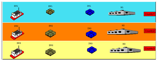
Figure 1.
Illustration of the three-country supply chain (adapted from [3]).
- A production plant (PPi),
- An export warehouse (EWi),
- An import warehouse (IWi),
- A final market ().
Customerdemands originate at each market . When a demand arrives, the decision-maker must choose between two broad fulfillment routes:
- Domestic route—ship directly from the same country’s export warehouse EWi; this option avoids tariffs and involves only short, low-cost transport, but is limited by the available stock in EWi.
- Cross-border route—import the item from another country’s export warehouse EWj (). This choice triggers additional transportation time, tariff charges at the destination country, and extra pipeline inventory costs.
Both routes are further constrained by finite warehouse capacities; once a warehouse is full, incoming production must wait, and once it is empty, certain routing options become infeasible. These capacity limits are explicitly captured in the stock component of the SMDP state, making inventory management an integral part of the reinforcement learning decision process.
4.2. Cost Formulation and Parameter Settings
To capture the principal trade-offs in this global network, we modeled production costs, transportation costs, inventory holding costs, and late delivery penalties, alongside tariff expenses for cross-border movements. The total time to fulfill an order encompassed both production lead time and transportation time, each of which followed a specified probability distribution. Our baseline exchange rate intervals and the uniform 15% tariff were taken directly from the benchmark study of Pontrandolfo et al. [3], so that subsequent scenario variations remained comparable to an established data set.
Below, we summarize the primary parameters and their role in our SMDP model:
- Exchange Rates (). Each country’s currency converts into the reference monetary unit (MU) via
- Sale Price (P). The list price is fixed at MU (monetary unit); selling in country j therefore yields .
- Production Cost (M). A unit produced in country i costs in MU with LU (local currency units).
- Inventory Holding Cost (). Baseline carrying charge MU per unit-time, rescaled by the country-specific storage factors and the sensitivity multiplier introduced in Section 6.
- Transportation Cost and Time. Let be the shipping charge for an order routed from origin i to destination j and be its transit time:
- Domestic (): , .
- Cross-border, slow (): , .
- Cross-border, fast (): , .
- Pipeline Cost Rate (C). A running charge of MU per time unit is applied while the shipment is in transit.
- Tariff Rate (). A uniform ad-valorem duty applies to every cross-border movement (). Baseline for Scenarios 1 and 2; Scenario 3 adopts country-specific rates .
- Late-Delivery Penalty (L). If total lead time tu, a penalty of with MU is incurred.
- Production Lead Time (). Drawn i.i.d. from time units.
Revenue/Reward Calculation. Suppose an item is produced in country i and shipped to country j. The net gain in the implementation is derived by the following equation. In (3) the large bracket groups together (i) the production cost, (ii) the pre- and post-production inventory charges and , (iii) the fixed freight fee , and (iv) the time-proportional pipeline cost incurred while the item is in transit. The two indicator functions and evaluate to 1 when the shipment is, respectively, cross-border and late; they are 0 otherwise. All symbols appearing in the reward expression are summarized in Table 1.

Table 1.
Notation used in the landed-cost and reward expressions.
Illustrative Calculation
Using the baseline values , , , , , , and and the instance with , with , , and tu, while assuming that the shipment arrives on time (), (3) becomes
Even after accounting for production, two holding phases, pipeline cost, and a 15% tariff, the high destination exchange rate () still yields a healthy profit of ≈649 MU for this single order.
4.3. SMDP States and Actions
- Destination Country Logic:
Let i be the originating country and a the chosen action. We define the destination country j as follows:
- Action 0: Local Shipping.
- If (Country 1):
- Action 1 or 2 → shipping from Country 2 (), where Action 1 indicates slow shipping and Action 2 indicates fast shipping.
- Action 3 or 4 → shipping from Country 3 (), where Action 3 is slow and Action 4 is fast.
- If (Country 2):
- Action 1 or 2 → shipping from Country 1 (), with Action 1 for slow and Action 2 for fast.
- Action 3 or 4 → shipping from Country 3 (), with Action 3 for slow and Action 4 for fast.
- If (Country 3)::
- Action 1 or 2 → shipping from Country 1 (), with Action 1 for slow and Action 2 for fast.
- Action 3 or 4 → shipping from Country 2 (), with Action 3 for slow and Action 4 for fast.
4.4. Scenario Setup
Using these parameters and definitions, we investigated how an RL-based SMDP model adapted under different global conditions. Specifically, we examined three key scenarios:
- Replication of Pontrandolfo et al. [3] —adopting their original exchange rate distributions and a uniform tariff of 0.15.
- Narrowed Currency Gap—modifying the exchange rate ranges to be more closely aligned among the three countries.
- Differentiated Tariffs—imposing distinct duty rates per country to assess how tariff disparities shape sourcing decisions.
By contrasting these scenarios, we demonstrate how even moderate shifts in exchange rates or import duties can significantly alter global supply chain strategies. In the next section, we detail our RL-based methodology (SMART) for deriving near-optimal policies within this SMDP framework.
4.5. Setup and Implementation
We began our analysis with a three–country baseline in which each country’s demand process followed the same Erlang distribution with moderate variability. Specifically, we set the shape parameter and scale , yielding an average inter-arrival time of and a coefficient of variation . For the robustness experiments introduced later, we additionally explored “heavy-tailed’’ demand with () and “light’’ demand with (); the implementation merely replaced the shape parameter k when launching those runs. The code leveraged the simpy simulation library to generate demand arrivals, applied a Q-learning (RL) update (SMART-style) for each incoming demand, and ran the simulation for time units.
Each demand arrival triggers a state lookup: we identified the state; selected an action via -greedy; computed the resulting reward based on production and shipping costs, tariffs, and inventory holding; and then updated the Q-table.
5. Comparisons and Overall Discussion
We investigated three scenarios, each reflecting a different combination of exchange rate distributions and tariff structures. Below, we recap the findings from each scenario and then discuss the overarching insights, including a validation experiment using Deep Q-Networks (DQNs).
All simulation notebooks, trained models, and auxiliary artifacts underlying the present work are archived on Zenodo (Yilmaz Eroglu (2025)) [39].
5.1. Validation
Although our main solution utilized a Q-learning method, we also employed a Deep Q-Network (DQN) to validate that the learned policy was robust, aligning with more advanced function-approximation approaches [25]. DQN replaced the Q-table with a neural network and used experience replay and target networks to stabilize training [27,28,29]. We tested the same three scenarios using both Q-learning and DQN under identical cost structures and demand processes, comparing their average rewards () over simulation time.
The tabular-versus-DQN run reported below was executed under Scenario 1. We fixed the demand process at and ran each learner for a 500 tu horizon.
- Quantitative comparison (Table 2).
Table 2 brings together six performance indicators for the stock-level grid . The SMART lookup table () out-earns its neural counterpart () at every size, with absolute gaps of 4–7 MU. Overlap% is the share of the 450 state–action pairs whose greedy action under DQN matched the SMART optimum; even when the reward gap was large, DQN still agreed with SMART on at least one state in eight and on almost 60% of the states at . MSE quantifies the mean-squared deviation between the two Q–tables (reported in ); its sharp fall from to confirmed that the network approximation improved as the state grid became denser. Both learners converged within a single 10 k epoch episode (Conv. ep.) across the full range, indicating efficient learning for problems up to .
Table 2.
Quantitative comparison of tabular Q-learning vs. DQN (500 tu horizon, ≈300 arrivals).
Table 2.
Quantitative comparison of tabular Q-learning vs. DQN (500 tu horizon, ≈300 arrivals).
| Overlap (%) | MSE | Conv. Ep. (T/D) | |||
|---|---|---|---|---|---|
| 5 | 20.82 | 16.10 | 13.3 | 21.6 | 1/1 |
| 10 | 25.25 | 21.05 | 40.0 | 5.1 | 1/1 |
| 20 | 20.63 | 13.93 | 11.7 | 2.2 | 1/1 |
| 30 | 21.09 | 15.60 | 57.8 | 1.2 | 1/1 |
- Dynamic behavior (Figure 2).
Figure 2 tracks the on-line estimate of the long-run average reward over the first 300 demand arrivals (≈500 simulation time units). Solid lines show SMART; dashed lines show the corresponding DQN runs. All trajectories exhibit an initial exploration spike followed by damped oscillations and stabilization. For every , the SMART curve settled earlier and higher, illustrating its sample-efficiency advantage: each interaction updated the exact state–action cell, whereas the DQN needed to rely on mini-batch gradients to shape its value function.
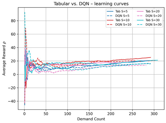
Figure 2.
Learning curves of tabular Q-learning (solid) versus DQN (dashed) for stock level sizes . Horizontal axis: cumulative Demand Count; vertical axis: on-line estimate of .
Figure 2.
Learning curves of tabular Q-learning (solid) versus DQN (dashed) for stock level sizes . Horizontal axis: cumulative Demand Count; vertical axis: on-line estimate of .
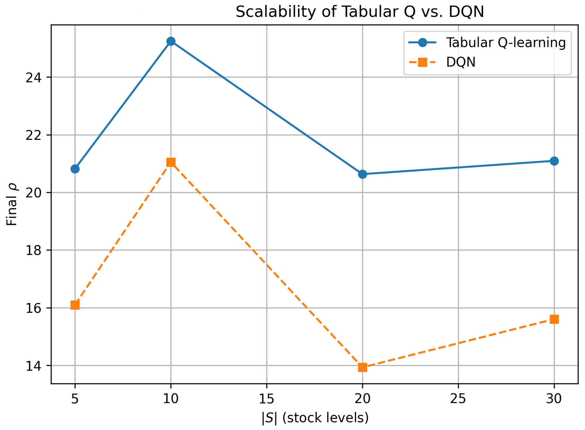
- Scalability snapshot (Figure 3).
Figure 3 distils the end-point data of Figure 2 into a single scalability plot: final versus . SMART dominated across the entire range, peaking at and losing only four MU when the state space tripled to . DQN peaked at the same point but its profit dropped sharply (by more than 7 MU) at and recovered only marginally at . Hence, within realistic warehouse capacities () a tabular policy was simultaneously more interpretable and more profitable than a deeper, data-hungry alternative.
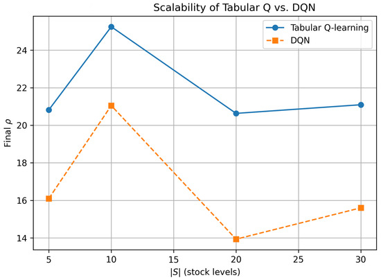
Figure 3.
Scalability of tabular Q vs. DQN: final average reward after 500 tu as a function of .
Figure 3.
Scalability of tabular Q vs. DQN: final average reward after 500 tu as a function of .
The long-run average rewards in Table 2 and Figure 2 and Figure 3 are purposely higher (about 20– for tabular) than those reported in the subsequent scenario analyses (about 8–). This is because the DQN-vs.-tabular benchmark was run for only 500 simulated time units (≈300 demand arrivals) under Scenario 1’s wide exchange rate gap and a modest tariff, with no demand surges or transport disruptions. The short horizon limited inventory holding and late delivery penalties, while the large FX arbitrage inflated gross margins, together yielding a “best–case, warm-up snapshot” that was well suited for algorithmic comparison but not indicative of the steadier, lower-margin values observed over the 60,000–100,000 tu horizons analyzed later.
Given that warehouse policy limited stock discretization to and since tabular Q-learning outperformed DQN throughout this range, we retained the tabular SMART agent as the primary optimizer in all subsequent tariff and scenario analyses. DQN remained a secondary verification tool and a scalability reserve for potential future extensions where the state space would grow beyond the current operational bounds.
We analyzed three progressively restrictive policy experiments that varied exchange rate dispersion and tariff intensity in order to isolate their individual and joint effects on routing decisions. Scenario 1 adopted Pontrandolfo et al. [3]’s original settings—wide exchange rate bands (0.4–0.6, 0.9–1.1, 1.9–2.1) and a uniform 15% tariff—so that subsequent results were directly comparable to the seminal benchmark. Scenario 2 retained the 15% tariff but “compressed’’ the currency bands to (0.8–1.0, 0.9–1.1, 0.7–0.9), mirroring the purchasing power parity spreads typical of OECD and upper-middle-income currencies in the 2024 Big-Mac Index [40]. Frequent tariff interventions during the 2018–2019 U.S.–China dispute clustered around 10% and 15%, with 25% emerging as the upper end of actual policy moves [41]. Scenario 3 therefore retained 10% and 15% as “realistic” tiers and introduced a 30% ceiling—just above the observed 25%—to stress-test the model under a plausibly extreme, yet policy-relevant, shock.
Figure 4 shows that the tabular SMART learner reached a stable, long-run average reward under each exchange rate/tariff scenario before any policy comparisons were made, thus complementing the earlier DQN cross-validation and ensuring that subsequent results were based on steady-state, not transient, behavior. Figure 4 tracks the long-run average reward per episode, where one episode was defined as 10,000 consecutive decision epochs (production–shipment cycles). Bundling raw epochs into fixed-length episodes served two purposes: (i) it produced a smooth, interpretable curve that was independent of the highly variable physical time a single epoch may cover in a semi-Markov setting; (ii) it allowed us to apply a pragmatic stopping rule—training was halted once the absolute change in between two successive episodes fell below 1% of the previous value.
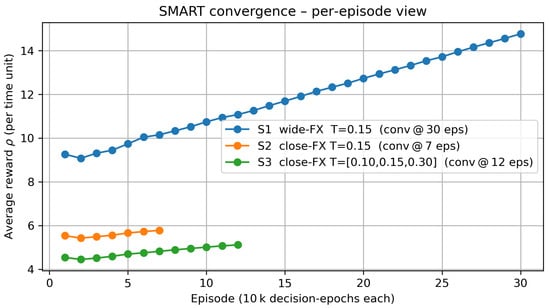
Figure 4.
Convergence behavior of the SMART learner. Each point represents the long-run average reward after one episode of 10,000 decision epochs (arrivals → actions → stochastic lead times). Convergence was declared once the drift between two consecutive episodes fell below 1 %.
To put the 100,000 simulated time-unit (tu) horizon used in the main experiments into perspective, recall that customer demand in each country followed an Erlang process with shape–scale parameters ; hence, the mean inter-arrival time was . Over 100,000 tu, each country therefore generated on average 100,000/5 = 20,000 arrivals. Because the three national markets operated independently, the system as a whole experienced approximately 3 × 20,000 ≈ 60,000 decision epochs, where one decision epoch was defined as“arrival → action choice → stochastic lead-time realization’’ and triggered a single Q-value update. For monitoring purposes, we bundled these raw epochs into fixed episodes of 10,000 decision epochs each; consequently, 100,000 tu corresponded to about 60,000/10,000 ≃ 6 episodes. This back-of-the-envelope calculation justified the six-episode convergence windows shown in Figure 4.
Under these conditions the SMART learner converged in 7, 12, and 30 episodes for Scenarios 2, 3, and 1, respectively. Scenario 1, which featured large exchange rate differentials, exhibited a prolonged upward drift because the agent continued to exploit profitable cross-border arbitrage as it received more experience. By contrast, Scenario 2 and Scenario 3 stabilized much earlier, reflecting a flatter cost landscape and the dampening effect of tariffs on exploratory re-routing. The steady-state reward hierarchy visible on the last points of each curve corroborated the policy performance comparisons. Note that the largest run (Scenario 1, 30 episodes) still fit well within the global simulation horizon of 100,000 time units adopted throughout this study, confirming that all performance metrics were obtained from a fully converged Q-table.
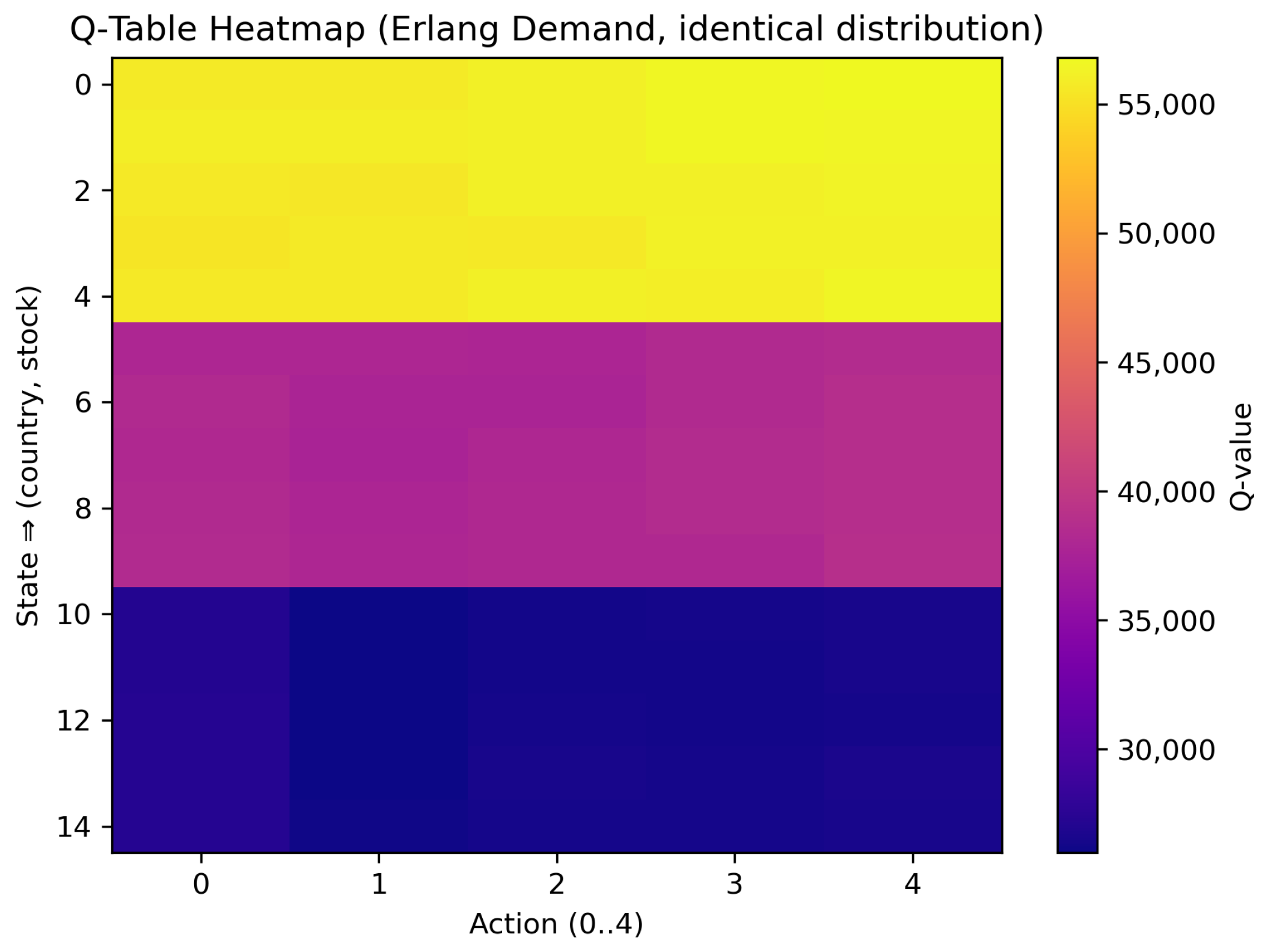
5.2. Scenario 1: Erlang Demand with Uniform Tariffs
In this baseline scenario, countries faced wide exchange rate gaps (e.g., 0.4–0.6, 0.9–1.1, 1.9–2.1) but a single uniform tariff (T = 0.15). The resulting Q-table is presented in Table 3 and a heatmap appears in Figure 5.
Table 3.
Scenario 1 Q-table results (uniform tariff, wide exchange gaps).

Figure 5.
Scenario 1 heatmap. Each row corresponds to one (country, stock) state; columns are actions . High values (yellow) favor shipping from or to high-exchange-rate regions.
In Table 3, the final column labeled bestAction gives , that is, the index of the action that yielded the highest long-run average reward for the corresponding state. Action 0 denoted local shipping, whereas Actions 1–4 denoted cross-border shipping with slow (1, 3) or fast (2, 4) transit, as defined in the previous subsection. Hence, bestAction 3 or 4 indicated that the agent preferred to import from the high-exchange-rate country via the specified mode. Figure 5 visualizes the same Q-learning table as a heatmap. A prominent block-wise gradient appears from rows 0–4 to rows 10–14: bright yellow bands correspond to Country 1 (the most favorable exchange rate range), magenta tones to Country 2, and deep indigo to Country 3. Within each five-row block (fixed country), color shades are almost uniform, confirming that, in this scenario, stock level had only a second-order effect on the learned Q-values; the dominant gradient was the block-wise shift caused by the large exchange rate differences across countries.
Our major observations were
- Country 1 and Country 2 frequently selected actions associated with cross-border shipping from Country 3 (e.g., bestAction = 3 or 4) to exploit Country 3’s high exchange rate, offsetting the uniform tariff cost.
- Country 3 predominantly used action 0, indicating that local fulfillment was most profitable when exchange rate advantages were already in its favor.
- The agent achieved an average reward consistent with the previous literature’s wide-gap scenarios, validating the RL approach in this baseline setting.
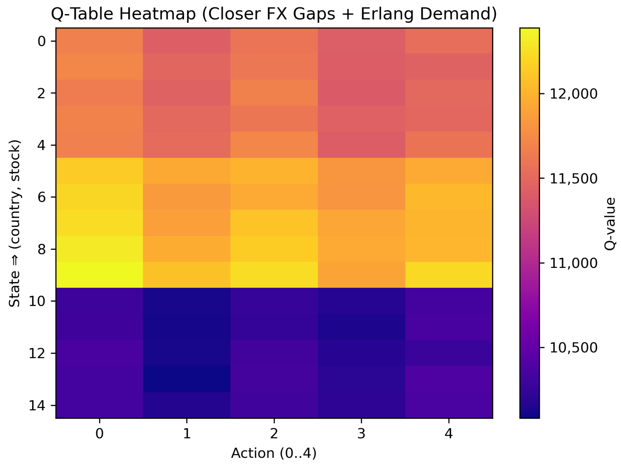
5.3. Scenario 2: Closer Exchange Rates
Here, we narrowed the currency ranges to while keeping the tariff rate at T = 0.15. As displayed in Table 4 and Figure 6, the net-revenue advantage of cross-border shipments was markedly smaller than in Scenario 1.
Table 4.
Scenario 2 Q-table results (closer exchange rates, uniform tariff).
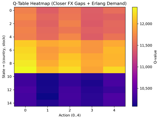
Figure 6.
Scenario 2 heatmap (closer exchange rates).
Table 4: The Q-values here lay in a much tighter band—roughly 10,100 to 12,400 monetary units—showing that exchange rate differences contributed less to overall profitability. The bestAction column revealed a strong shift toward local fulfillment: Country 1 selected Action 0 in three of five stock states; Country 2 chose local shipping in all states; Country 3 overwhelmingly chose the fast cross-border alternative (Action 4) in four out of five stock states; the sole exception was the mid-stock level (s = 2), where local fulfillment (action 0) became marginally more rewarding.
In Figure 6, the color scale ranged from around 10,100 (deep indigo) to 12,400 (bright yellow). Compared with Figure 5, the horizontal block-wise contrast across countries was less pronounced; instead, subtle vertical striations indicate that the choice between slow (actions 1, 3) and fast (actions 2, 4) cross-border modes was here cost-neutral in many states. Overall, the flattened Q-value landscape confirms that narrowing the currency gap reduced the economic incentive for cross-border sourcing, thereby encouraging more local or balanced strategies across the three-country network.
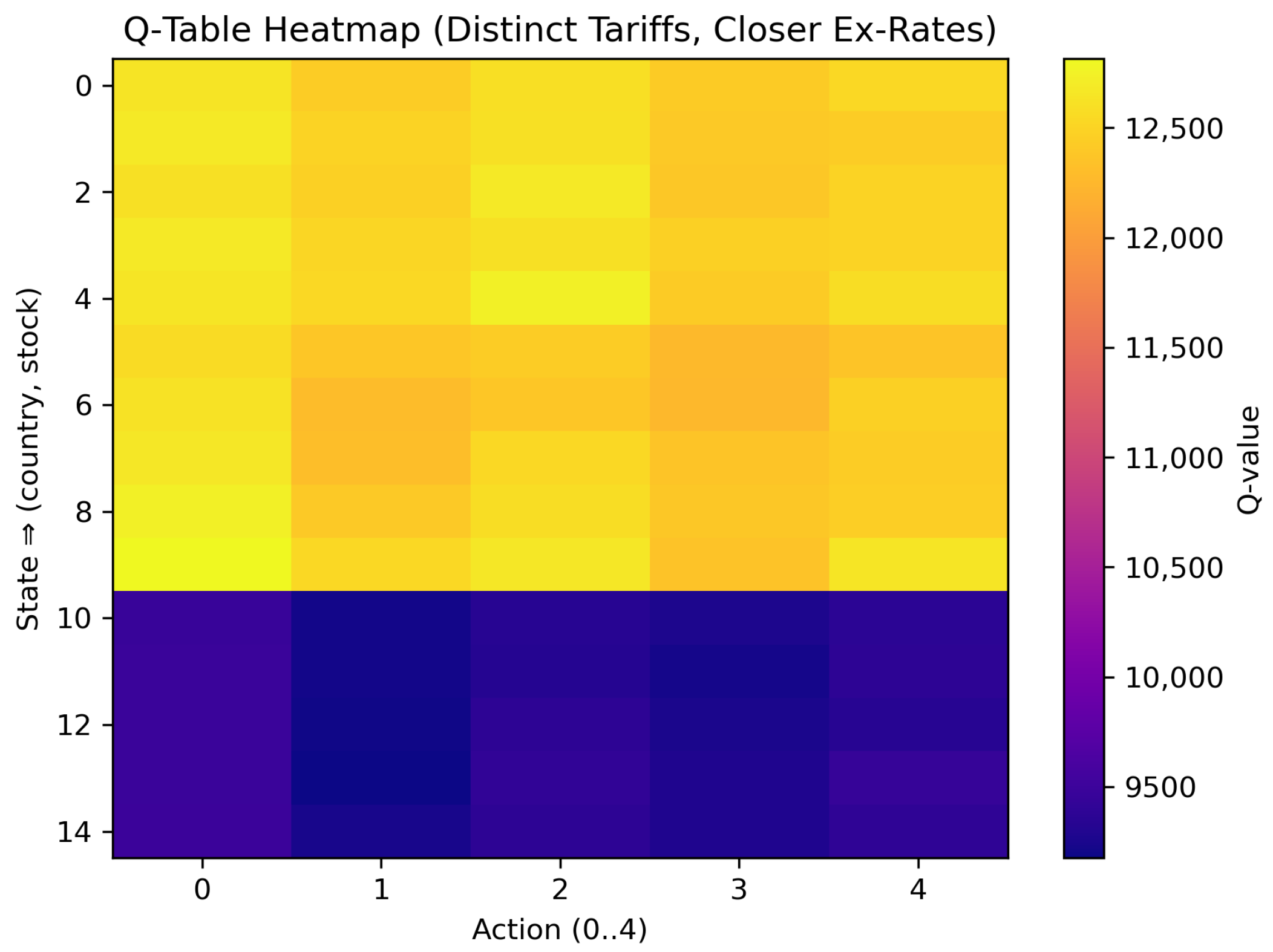
5.4. Scenario 3: Distinct Tariffs with Closer Exchange Rates
Finally, we introduced distinct tariffs for each origin country, e.g., , , while retaining the narrower currency intervals.
As summarized in Table 5 and visualized in Figure 7, the color scale now ran from roughly 9100 (deep indigo) to 12,750 (bright yellow) monetary units, representing a wider band than in Scenario 2. This broader spread confirmed that the introduction of heterogeneous tariffs—rather than the already-narrow exchange rate differences—became the dominant source of Q-value variation. The bestAction column shows a strong preference for local fulfillment (Action 0) in Countries 1 and 2, with only two fast cross-border selections (Action 2) for Country 1 at stock levels and . Country 3 never chose a cross-border option; its 30% export tariff fully canceled any residual currency edge. Correspondingly, rows 0–9 in Figure 7—representing Countries 1 and 2—display warm yellow or orange cells under Action 0, whereas rows 10–14 (Country 3) remain uniformly violet, highlighting the profitability gap induced by the tariff differential. Vertical shading differences between slow (Actions 1 and 3) and fast (Actions 2 and 4) cross-border modes are faint, indicating that these intra-origin transit-time effects were secondary to the tariff impact.
Table 5.
Scenario 3 Q-table results (closer exchange rates, distinct tariffs).
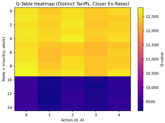
Figure 7.
Scenario 3 heatmap (distinct tariffs, closer exchange rates).
Table 5 and Figure 7 demonstrate how imposing heterogeneous origin tariffs reshaped the learned policy: the Q-value landscape was here segmented primarily by tariff level rather than by the modest exchange rate differences, leading to the following country-specific patterns.
- Country 1 showed significant variation between local (Action 0) and cross-border (particularly Action 2 or 4) shipping. The interplay of moderate exchange gain versus partial tariff led to nuanced decisions.
- Country 2 mostly remained local as the distinct tariff structure seldom warranted cross-border shipping unless a modest inventory shortage arose.
- Country 3, facing the highest tariff outflow (0.30), rarely found cross-border shipping profitable; nearly all states yielded bestAct = 0, preserving local supply.
6. Discussion and Conclusions
6.1. Baseline Design: Three Currency–Tariff Scenarios
Through the three scenarios presented, we demonstrate how a reinforcement learning (RL) approach (SMART) adapts its fulfillment strategy in response to varying exchange rate gaps and tariff rules.
- Wide exchange gaps + uniform tariffs (Scenario 1): Encourage cross-border shipping from the highest-exchange-rate country (Country 3), provided inventory or lead-time constraints do not override the advantage.
- Closer exchange rates (Scenario 2): Reduce the incentive for cross-border shipments, promoting more local or balanced sourcing while showing how a smaller currency gap can shift strategies away from a single dominant supplier.
- Distinct tariffs (Scenario 3): Further complicate the cost landscape by discouraging exports from countries with steep tariffs (e.g., 0.30 for Country 3), although local vs. global choices may still hinge on inventory levels and lead-time risks.
Although the baseline three-scenario matrix already captured the most salient cost drivers, exchange rate gaps, and tariff heterogeneity, real-world supply chains face additional stochastic shocks such as demand surges and in-transit disruptions. To verify that our RL controller remains effective under such noise, we augmented each baseline configuration with a carefully chosen set of uncertainty-extended variants. The resulting six-scenario suite, documented in Table 6 and visualized in Figure 8, allowed us to confirm that all qualitative insights obtained from the lean three-scenario design continued to hold once these extra uncertainties were switched on.
6.2. Scenario Exploration: Baseline vs. Uncertainty-Extended Variants
To probe the robustness of the Smart reinforcement learning controller, we expanded the original three scenarios (wide-gap exchange rates, closer exchange rates, and distinct tariffs) with three uncertainty-extended counterparts that injected (i) stochastic supply disruptions and (ii) demand-arrival variance via alternative parameters. The complete six-scenario design is summarized in Table 6.
All six scenarios shared the same cost structure, yet three extended variants injected additional randomness along two orthogonal axes:
- Demand . We modeled inter-arrival times with a Gamma distribution whose shape k directly controlled variance while leaving the mean unchanged.
- (baseline): moderate variability.
- (“light”): thinner tail → smoother workload.
- (“heavy”: thicker tail → bursty arrivals, mimicking demand shocks.
- Supply disruption (10 tu delay, p = 0.10). With a probability of , every shipment received an additional 10 time-unit transit penalty, representing port congestion, customs holds, or transport breakdowns. The penalty was large enough to trigger the model’s late delivery cost in many episodes, thereby stressing the learning agent.
Why these extensions matter. They broadened the uncertainty set from purely price-driven shocks (exchange rates and tariffs) to operational and market shocks: variable customer demand and stochastic pipeline delays. The red, violet, and brown trajectories in Figure 8 demonstrate that despite noticeably higher volatility in , the ordering of profit performance remained intact. Hence, the core managerial insights reported for the lean three-scenario design were robust to these extra real-world complications, justifying our decision to keep the subsequent policy experiments focused on Scenarios 1–3 only.
Table 6.
Definition of the six simulation scenarios.
Table 6.
Definition of the six simulation scenarios.
| Scenario Label | Exchange Rate Range | Tariff Rule | Demand | Supply Disruption |
|---|---|---|---|---|
| Scenario 1 | uniform 0.15 | (baseline) | – | |
| Scenario 2 | uniform 0.15 | – | ||
| Scenario 3 | same as Sc. 2 | [0.10, 0.15, 0.30] | – | |
| Scenario 1 (+Ext) | same as Sc. 1 | uniform 0.15 | (heavy) | 10 tu delay, |
| Scenario 2 (+Ext) | same as Sc. 2 | uniform 0.15 | (light) | 10 tu delay, |
| Scenario 3 (+Ext) | same as Sc. 2 | [0.10, 0.15, 0.30] | 10 tu delay, |
Figure 8.
Long-run average reward under six scenarios. Each curve tracks versus cumulative demand arrivals. Scenarios 1–3 (solid blue, orange, green) reproduced the baseline exchange rate/tariff settings; their uncertainty-extended counterparts (red, violet, brown) added heavy-tailed or light-tailed demand and a 10 time-unit (tu) disruption that occurred with a probability of .
- What the trajectories reveal.
Figure 8 confirms three consistent patterns.
- (i)
- Currency advantage dominated. After injecting heavy demand variance and 10 tu supply delay shocks, Scenario 1 (+Ext) still produced the highest long-run reward. Country 3 retained the strongest currency (exchange rate interval –), so shipping from Country 3 remained profitable enough to outweigh both the uniform tariff and the extra disruptions. The extended demand process () simply lengthened the horizontal axis—more demands were realized—thereby stretching the trajectory far to the right and letting climb above 9.7.
- (ii)
- Narrower gaps compressed profit. Both baseline and extended versions of Scenario 2 plateaued at around . Here, the three exchange rate intervals overlapped (–), so cross-border arbitrage was weak; the lighter arrival variance case () only added marginal noise without changing the level.
- (iii)
- Steep tariffs remained binding. Scenario 3 trajectories settled roughly one unit below Scenario 2. The country-specific tariffs [0.10, 0.15, 0.30] penalized exports from the high-currency regions, and the added disruption risk in the extended variant reduced a little further.
Because the extended variants preserved the qualitative ordering , we retained the lean three-scenario set to streamline the policy experiments, while Figure 8 shows that the conclusions were robust to additional real-world uncertainties.
6.3. Sensitivity Analysis
6.3.1. Sensitivity to Quantity Discounts
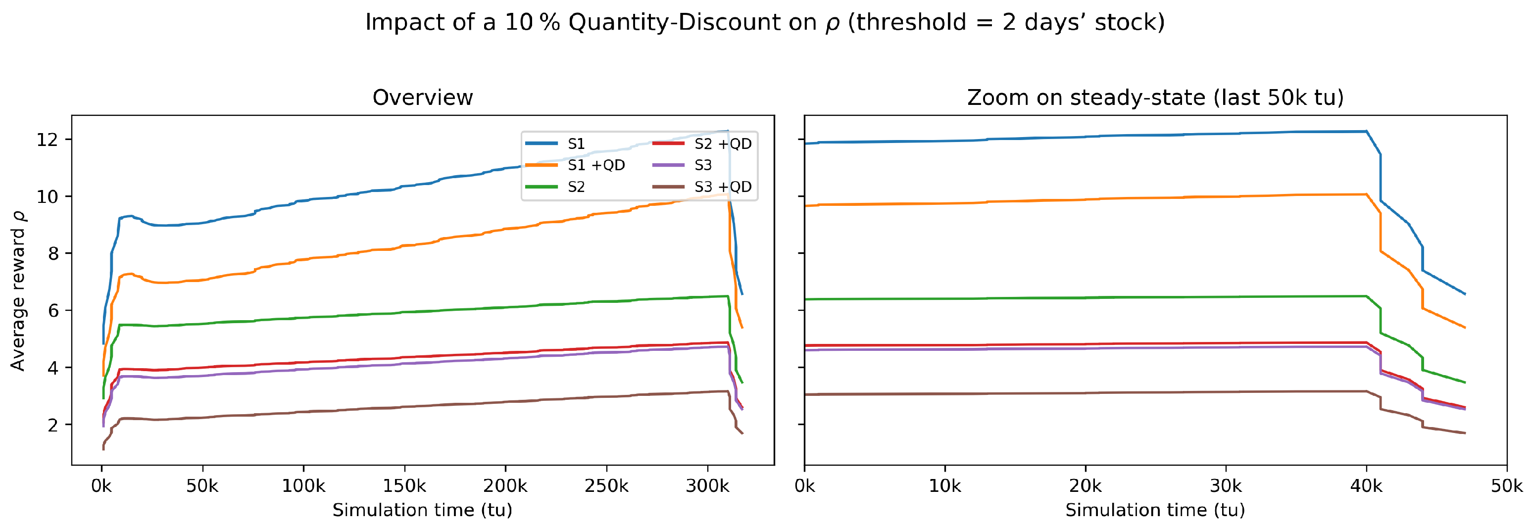
Real-world procurement contracts often feature volume-based rebates; to examine whether such price incentives altered our policy insights, we re-ran the baseline exchange rate/tariff design under a 10% quantity discount that was triggered once on-hand inventory exceeded two days of expected demand. The threshold = units, matching the Erlang- arrival rate. The six resulting trajectories—three original scenarios with and without a discount—are plotted in Figure 9. Across all cases, the discount depressed the long-run average reward by roughly 15–20% yet preserved the ordering . Hence, the managerial conclusions derived from the lean three-scenario framework remained robust; the subsequent sections therefore continued to focus on Scenarios 1–3 without loss of generality.
Figure 9.
Impact of a 10% quantity discount on the long-run average reward . Each colored pair represents one of the three exchange rate/tariff scenarios: the first entry (S1–S3) is the baseline, whereas the matching label with “+QD” shows the outcome when the 10% discount was triggered once on-hand stock exceeded two days of expected demand. The (left panel) depicts the entire 300 k tu horizon; the (right panel) zooms into the final 50 k tu to highlight steady-state differences between the baseline and discount runs. The symbol “k tu’’ abbreviates thousand time units (e.g., 50 k tu = 50,000 simulation time units).
6.3.2. Sensitivity to Tariff
To quantify how strongly the Smart policy reacted to tariff shocks, we re-ran the baseline exchange rate design while systematically varying a uniform ad valorem tariff applied to every cross-border shipment. The sweep covered tariff grid ; each run spanned (steady state reached ≳ 80% of the horizon). to in steps of for all three scenarios:
- Scenario S1—wide: large exchange rate gaps, uniform baseline tariff .
- Scenario S2—close: compressed exchange rates, uniform tariff.
- Scenario S3—tariff–vec: same exchange rates as S2 but country-specific baseline tariffs; when swept, the same was imposed on every lane for comparison.
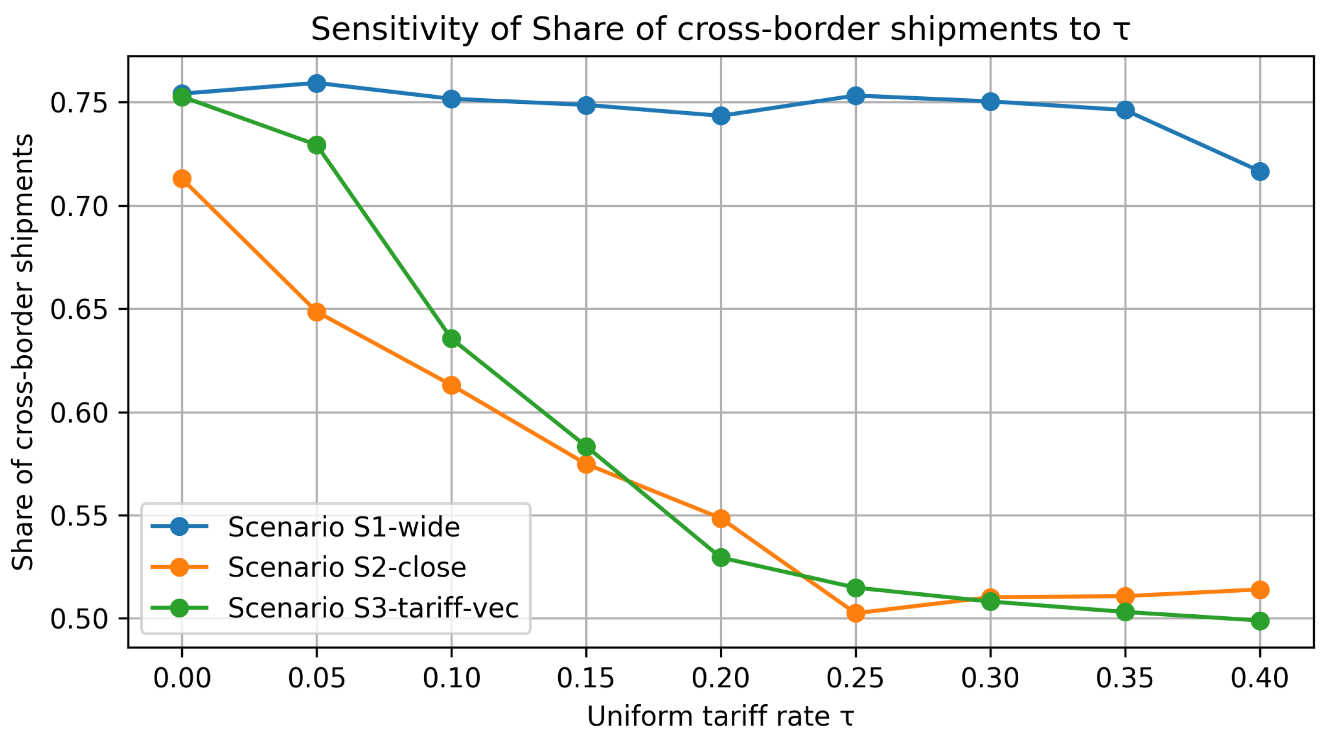
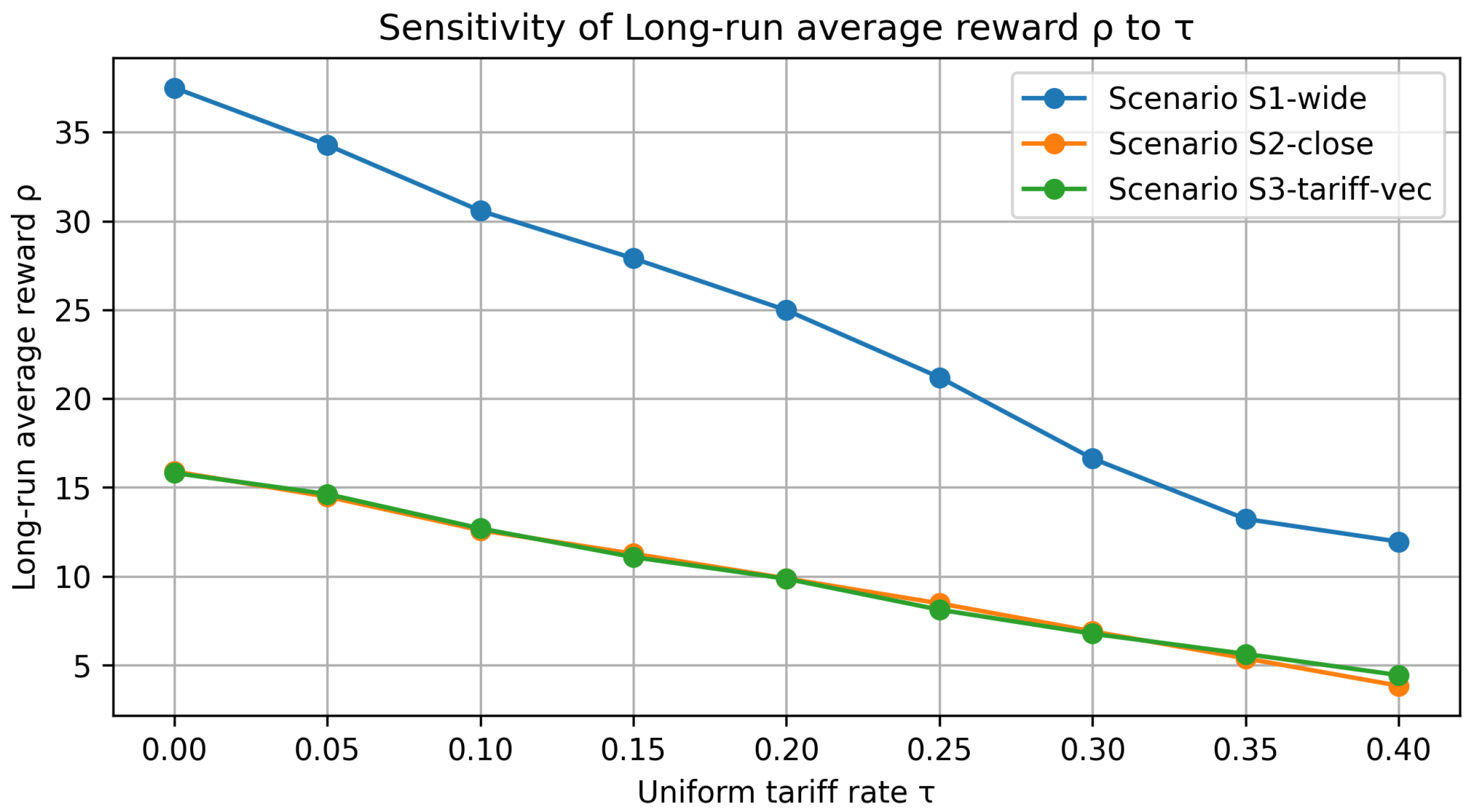
Figure 10 tracks the share of cross-border shipments (international orderstotal), whereas Figure 11 displays the resulting long-run average reward under the same tariff grid.
Figure 10.
Tariff sensitivity of the cross-border shipment share. All curves slope downward: higher uniform tariffs discouraged global fulfillment. S1 (large currency gaps) remained the most internationalized (75% at ; still 70% at ), while S2 and especially S3 pivoted sharply toward domestic sourcing once .
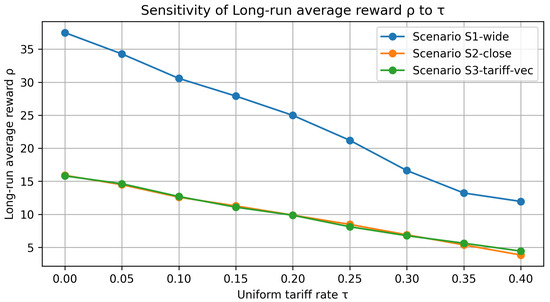
Figure 11.
Tariff sensitivity of the long-run average reward . Profit declined roughly linearly with . Wide currency advantages (S1) buffered the loss, yet dropped by ∼65% over the sweep. S2 and S3 converged, showing that once currency gaps were narrow, any tariff materially eroded margins.
Figure 10, cross-border share under rising tariffs: The plot tracks the share of orders that the Smart policy fulfilled via cross-border shipments as the ad valorem tariff increased from 0 to 40%. For the wide-gap exchange rate setting (Scenario 1, solid blue) the currency advantage was so strong that the policy kept more than 80% of flows international until tariffs exceeded about 25%; only beyond that point did the curve slope down more steeply. By contrast, the closer-gap baseline (Scenario 2, orange) and the distinct tariff case (Scenario 3, green) were far more sensitive: their curves crossed the “half-and-half’’ line (50% cross-border share) around the mark, confirming the reviewer’s intuition that a 30% duty was a decisive threshold for reshaping fulfillment toward local sources.
Figure 11—profit impact of tariff escalation: The panel converts the uniform tariff sweep into long-run average reward (MU tu−1). All three scenarios followed an almost linear downward trend, yet with clearly distinct slopes. Scenario 1, protected by the wide exchange rate gap, still posted the highest margins but surrendered about 6 MU of for every ten-percentage-point (10 pp) increase in the ad valorem duty. By contrast, Scenarios 2 and 3—whose currency bands were compressed—lost roughly 2.5–3 MU per 10 pp; the slightly steeper gradient of Scenario 3 reflects the extra asymmetry introduced by its country-specific baseline tariffs. Taken together, the sourcing-mix plot (Figure 10) and the curve shown here demonstrate that both network routing and overall profitability pivoted decisively once tariffs crossed the 25–30% band, thereby pinpointing the policy threshold at which cross-border procurement ceased to be economically attractive.
Key take-aways. (i) Tariffs reshape fulfilment choices primarily by throttling the volume of cross-border moves (Figure 10); profit effects (Figure 11) are a second-order consequence. (ii) Scenario ordering persists for , but narrows considerably beyond that point. (iii) A uniform tariff of is sufficient to push the system toward near-autarky in otherwise balanced currency settings, underscoring how trade policy can overwrite exchange rate incentives.
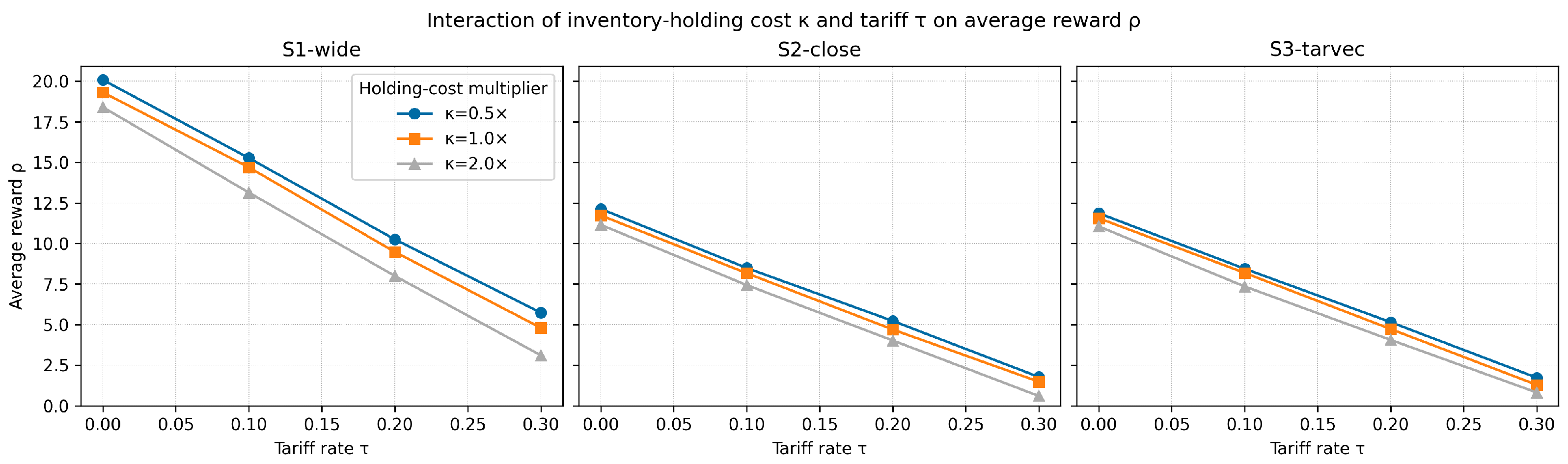
6.3.3. Joint Impact of Inventory Holding Cost and Tariff Level
Inventory carrying charges and customs duties are two of the most salient cost drivers in global fulfillment. To quantify their joint influence, we multiplied the baseline per-unit holding rate by and swept the uniform ad valorem tariff across , keeping all other parameters identical to Table 6. These two scalars entered the landed-cost expression already introduced in Equation (3): : origin/destination exchange rates; MU: unit production cost; : country-specific storage factors; MU per tu: in-transit cost rate; MU: list price; MU: late delivery penalty. The indicator activated the customs duty only for cross-border routes; triggered the late arrival charge whenever the realized pipeline time exceeded ten time units.
- Inventory multiplier rescaled both holding terms in Equation (3), i.e., the pre-production component and the post-shipment component .
- Tariff rate linearly scaled the customs-duty term .
Each pair was simulated for time units with average-reward Q-learning; the long-run reward was averaged over three macro-replications to attenuate noise. The results are summarized in Figure 12.

Figure 12.
Interaction of inventory holding cost and tariff on average reward . Columns correspond to the three exchange rate scenarios, while the three colored curves in each panel represent , , and the baseline holding rate. Markers denote the simulated levels; lines are visual guides.
Key observations. (i) Doubling or halving shifted the entire –curve almost in parallel, leaving its slope with respect to virtually unchanged, indicating that customs duties dominated stockholding charges in shaping landed cost. (ii) Increasing steeply reduced profit irrespective of , underscoring the primary role of duties in cross-border sourcing decisions. (iii) For every tested, the ordering remained intact, confirming that currency gaps and tariff structures were the principal levers, whereas inventory costs acted as a measurable—but second-order—modifier.
Managerial Insights: From a practical standpoint, global supply chain managers should continuously monitor tariff regulations and exchange rate fluctuations across potential sourcing countries. When tariffs spike or currency gaps narrow, previously optimal cross-border options might become suboptimal, emphasizing the need for agile decision-making and frequent policy updates. Having robust estimates for pipeline costs, lead-time risks, and inventory holding expenses further helps identify whether the gain from a cheaper supplier in another country still outweighs potential delays or tariff penalties.
To strengthen confidence in the learned policy, we also conducted a verification experiment using a Deep Q-Network (DQN). Although the tabular Q-learning (SMART) approach was simpler and highly interpretable for moderate-scale problems, the DQN results closely matched those of the tabular method, indicating that both methods respond similarly to changes in exchange rates and tariffs.
From Prototype to Shop-Floor Decision Support: While the foregoing results confirm the analytical value of the SMART learner, a key managerial question is whether such a policy can be embedded in day-to-day planning systems.
- Data pipeline. Most ERP suites already expose inventory levels and open purchase orders and inbound transit times. These feeds can populate the learner’s state vector in real time or on an hourly batch schedule.
- Training and inference layer. The SMART algorithm is lightweight enough to train overnight on a single CPU node. We therefore recommend a two-tier micro-service: (i) a nightly “trainer” container that ingests the previous day’s transactions and updates the Q-table; (ii) a stateless “inference” endpoint that is called by the ERP’s MRP run or by a /suggestRoute button in the buyer’s user interface.
- Power BI dashboard. Writing the live Q-table and KPIs (average reward, cross-border share, lead-time breach rate) to a cloud data-lake allows instant visualization in Power BI, Tableau, or Looker. Planners can “what-if” tariffs or exchange rates via slicers, triggering on-the-fly policy simulations without touching the production ERP.
- Governance and override. A simple traffic-light override is advisable: if the recommended action deviates from the incumbent rule or if the implied delivery date violates a service level agreement, the suggestion is pushed to an approval queue rather than executed automatically.
In short, the SMART learner can be surfaced as a thin decision-support layer—trained off-line, served on-line—that complements, rather than replaces, existing ERP logic. This architecture minimizes integration risk while giving managers a transparent, continuously improving view of how tariffs, exchange rate shifts, and pipeline costs jointly shape optimal fulfillment choices.
6.4. Limitations and Future Work
- (i)
- Modeling Scope. The prototype optimizes a single-product, single-echelon network without explicit capacity limits. Extending SMART to multiple SKUs (Stock-Keeping Units), regional DC (Distribution Center) layers, and finite production or transport capacities would require a constrained MDP formulation or a hierarchical multi-agent RL design. Future extensions could also account for sustainability metrics (e.g., CO2 cost per lane) and dynamic forecasting signals that update the MDP in real time.
- (ii)
- Stochastic Environment. Customer demand arrivals follow a stationary Erlang process, while all unit–cost coefficients (production, holding, pipeline, tariff, late penalty rates) are deterministic; uncertainty in the reward therefore arises only from demand timing, the stochastic production and transit times, and exchange rate fluctuations. Future research could relax these assumptions by introducing non-stationary demand patterns, volatile freight-rate schedules, and time-dependent quantity discount schemes.
- (iii)
- Computational Scalability. Tabular Q-learning suffices for the current 450 state–action pairs but does not scale to large state spaces. Preliminary Deep-Q results match the tabular policy; moving to will necessitate deeper networks, experience replay prioritization, and distributed training to maintain convergence speed.
Funding
This research received no external funding.
Data Availability Statement
All data generated and analyzed in this study are openly available on Zenodo (Yilmaz Eroglu (2025)) [39].
Conflicts of Interest
The author declares no conflicts of interest.
References
- Howard, R. Dynamic Probabilistic Systems, Volume II: Semi-Markov and Decision Processes; Jonh Wiley& Sons, Inc.: New York, NY, USA, 1971. [Google Scholar]
- Puterman, M.L. Markov Decision Processes: Discrete Stochastic Dynamic Programming; John Wiley & Sons: New York, NY, USA, 2014. [Google Scholar]
- Pontrandolfo, P.; Gosavi, A.; Okogbaa, O.G.; Das, T.K. Global supply chain management: A reinforcement learning approach. Int. J. Prod. Res. 2002, 40, 1299–1317. [Google Scholar] [CrossRef]
- Günay, E.E.; Park, K.; Okudan Kremer, G.E. Integration of product architecture and supply chain under currency exchange rate fluctuation. Res. Eng. Des. 2021, 32, 331–348. [Google Scholar] [CrossRef]
- van Tongeren, T.; Kaymak, U.; Naso, D.; van Asperen, E. Q-learning in a competitive supply chain. In Proceedings of the 2007 IEEE International Conference on Systems, Man and Cybernetics, Montréal, QC, Canada, 7–10 October 2007; IEEE: Piscataway, NJ, USA, 2007; pp. 1211–1216. [Google Scholar]
- Chaharsooghi, S.K.; Heydari, J.; Zegordi, S.H. A reinforcement learning model for supply chain ordering management: An application to the beer game. Decis. Support Syst. 2008, 45, 949–959. [Google Scholar] [CrossRef]
- Zhao, X.; Sun, X. A multi-agent reinforcement learning approach for supply chain coordination. In Proceedings of the IEEE International Conference on Service Operations and Logistics, and Informatics (SOLI), Qingdao, China, 15–17 July 2010; pp. 341–346. [Google Scholar]
- Puskás, E.; Budai, Á.; Bohács, G. Optimization of a physical internet based supply chain using reinforcement learning. Eur. Transp. Res. Rev. 2020, 12, 47. [Google Scholar] [CrossRef]
- Rolf, B.; Jackson, I.; Müller, M.; Lang, S.; Reggelin, T.; Ivanov, D. A review on reinforcement learning algorithms and applications in supply chain management. Int. J. Prod. Res. 2023, 61, 7151–7179. [Google Scholar] [CrossRef]
- Zou, Y.; Gao, Q.; Wu, H.; Liu, N. Carbon-Efficient Scheduling in Fresh Food Supply Chains with a Time-Window-Constrained Deep Reinforcement Learning Model. Sensors 2024, 24, 7461. [Google Scholar] [CrossRef]
- Liu, J. Simulation of Cross-border E-commerce Supply Chain Coordination Decision Model Based on Reinforcement Learning Algorithm. In Proceedings of the 2023 International Conference on Networking, Informatics and Computing (ICNETIC), Palermo, Italy, 29–31 May 2023; IEEE: Piscataway, NJ, USA, 2023; pp. 429–433. [Google Scholar]
- Li, X.; Zheng, Z. Dynamic pricing with external information and inventory constraint. Manag. Sci. 2024, 70, 5985–6001. [Google Scholar]
- Gurkan, M.E.; Tunc, H.; Tarim, S.A. The joint stochastic lot sizing and pricing problem. Omega 2022, 108, 102577. [Google Scholar] [CrossRef]
- Li, X.; Li, Y. NEV’s supply chain coordination with financial constraint and demand uncertainty. Sustainability 2022, 14, 1114. [Google Scholar] [CrossRef]
- Bergemann, D.; Brooks, B.; Morris, S. The limits of price discrimination. Am. Econ. Rev. 2015, 105, 921–957. [Google Scholar] [CrossRef]
- Gomes, U.T.; Pinheiro, P.R.; Saraiva, R.D. Dye schedule optimization: A case study in a textile industry. Appl. Sci. 2021, 11, 6467. [Google Scholar] [CrossRef]
- Lu, C.; Wu, Y. Optimization of Logistics Information System based on Multi-Agent Reinforcement Learning. In Proceedings of the 2024 5th International Conference on Mobile Computing and Sustainable Informatics (ICMCSI), Lalitpur, Nepal, 18–19 January 2024; IEEE: Piscataway, NJ, USA, 2024; pp. 421–426. [Google Scholar]
- Kavididevi, V.; Monikapreethi, S.; Rajapriya, M.; Juliet, P.S.; Yuvaraj, S.; Muthulekshmi, M. IoT-Enabled Reinforcement Learning for Enhanced Cold Chain Logistics Performance in Refrigerated Transport. In Proceedings of the 2024 2nd International Conference on Sustainable Computing and Smart Systems (ICSCSS), Coimbatore, India, 10–12 July 2024; IEEE: Piscataway, NJ, USA, 2024; pp. 379–384. [Google Scholar]
- Zhou, T.; Xie, L.; Zou, C.; Tian, Y. Research on supply chain efficiency optimization algorithm based on reinforcement learning. Adv. Contin. Discret. Model. 2024, 2024, 51. [Google Scholar] [CrossRef]
- Liu, X.; Hu, M.; Peng, Y.; Yang, Y. Multi-agent deep reinforcement learning for multi-echelon inventory management. Prod. Oper. Manag. 2022, 10591478241305863. [Google Scholar] [CrossRef]
- Aboutorab, H.; Hussain, O.K.; Saberi, M.; Hussain, F.K.; Prior, D. Adaptive identification of supply chain disruptions through reinforcement learning. Expert Syst. Appl. 2024, 248, 123477. [Google Scholar] [CrossRef]
- Ma, N.; Wang, Z.; Ba, Z.; Li, X.; Yang, N.; Yang, X.; Zhang, H. Hierarchical Reinforcement Learning for Crude Oil Supply Chain Scheduling. Algorithms 2023, 16, 354. [Google Scholar] [CrossRef]
- Piao, M.; Zhang, D.; Lu, H.; Li, R. A supply chain inventory management method for civil aircraft manufacturing based on multi-agent reinforcement learning. Appl. Sci. 2023, 13, 7510. [Google Scholar] [CrossRef]
- Ma, Z.; Chen, X.; Sun, T.; Wang, X.; Wu, Y.C.; Zhou, M. Blockchain-based zero-trust supply chain security integrated with deep reinforcement learning for inventory optimization. Future Internet 2024, 16, 163. [Google Scholar] [CrossRef]
- Mnih, V.; Kavukcuoglu, K.; Silver, D.; Rusu, A.A.; Veness, J.; Bellemare, M.G.; Graves, A.; Riedmiller, M.; Fidjeland, A.K.; Ostrovski, G.; et al. Human-level control through deep reinforcement learning. Nature 2015, 518, 529–533. [Google Scholar] [CrossRef] [PubMed]
- Wang, Y.; Wang, J. Research on international logistics supply chain management strategy based on deep reinforcement learning. Appl. Math. Nonlinear Sci. 2024, 9, 13. [Google Scholar] [CrossRef]
- van Hasselt, H.; Guez, A.; Silver, D. Deep Reinforcement Learning with Double Q-Learning. In Proceedings of the AAAI Conference on Artificial Intelligence, Phoenix, AZ, USA, 12–17 February 2016. [Google Scholar]
- Wang, Z.; Schaul, T.; Hessel, M.; van Hasselt, H.; Lanctot, M.; de Freitas, N. Dueling Network Architectures for Deep Reinforcement Learning. In Proceedings of the 33rd International Conference on Machine Learning (ICML), New York, NY, USA, 19–24 June 2016; pp. 1995–2003. [Google Scholar]
- Schaul, T.; Quan, J.; Antonoglou, I.; Silver, D. Prioritized Experience Replay. In Proceedings of the International Conference on Learning Representations (ICLR), San Juan, PR, USA, 2–4 May 2016. [Google Scholar]
- Zhu, Z.; Lin, K.; Jain, A.K.; Zhou, J. Transfer learning in deep reinforcement learning: A survey. IEEE Trans. Pattern Anal. Mach. Intell. 2023, 45, 13344–13362. [Google Scholar] [CrossRef]
- Padhye, V.; Lakshmanan, K. A deep actor critic reinforcement learning framework for learning to rank. Neurocomputing 2023, 547, 126314. [Google Scholar] [CrossRef]
- Norouzi, A.; Shahpouri, S.; Gordon, D.; Shahbakhti, M.; Koch, C.R. Safe deep reinforcement learning in diesel engine emission control. Proc. Inst. Mech. Eng. Part J. Syst. Control Eng. 2023, 237, 1440–1453. [Google Scholar] [CrossRef]
- Prasuna, R.G.; Potturu, S.R. Deep reinforcement learning in mobile robotics—A concise review. Multimed. Tools Appl. 2024, 83, 70815–70836. [Google Scholar] [CrossRef]
- Rahimian, P.; Mihalyi, B.M.; Toka, L. In-game soccer outcome prediction with offline reinforcement learning. Mach. Learn. 2024, 113, 7393–7419. [Google Scholar] [CrossRef]
- Scarponi, V.; Duprez, M.; Nageotte, F.; Cotin, S. A zero-shot reinforcement learning strategy for autonomous guidewire navigation. Int. J. Comput. Assist. Radiol. Surg. 2024, 19, 1185–1192. [Google Scholar] [CrossRef]
- Liu, X.Y.; Xia, Z.; Yang, H.; Gao, J.; Zha, D.; Zhu, M.; Wang, C.D.; Wang, Z.; Guo, J. Dynamic datasets and market environments for financial reinforcement learning. Mach. Learn. 2024, 113, 2795–2839. [Google Scholar] [CrossRef]
- Yu, L.; Guo, Q.; Wang, R.; Shi, M.; Yan, F.; Wang, R. Dynamic offloading loading optimization in distributed fault diagnosis system with deep reinforcement learning approach. Appl. Sci. 2023, 13, 4096. [Google Scholar] [CrossRef]
- Sutton, R.S.; Barto, A.G. Reinforcement Learning: An Introduction; MIT Press: Cambridge, MA, USA, 1998; Volume 1. [Google Scholar]
- Yilmaz Eroglu, D. RL for Multi-Country Supply-Chains (Q-Learning & Deep Q-Network); Zenodo: Geneva, Switzerland, 2025. [Google Scholar] [CrossRef]
- The Economist. The Big Mac Index—January 2024. Available online: https://github.com/TheEconomist/big-mac-data/releases/tag/2024-01 (accessed on 15 July 2025).
- Jeanne, O.; Son, J. To what extent are tariffs offset by exchange rates? J. Int. Money Financ. 2024, 142, 103015. [Google Scholar] [CrossRef]


Disclaimer/Publisher’s Note: The statements, opinions and data contained in all publications are solely those of the individual author(s) and contributor(s) and not of MDPI and/or the editor(s). MDPI and/or the editor(s) disclaim responsibility for any injury to people or property resulting from any ideas, methods, instructions or products referred to in the content. |
© 2025 by the author. Licensee MDPI, Basel, Switzerland. This article is an open access article distributed under the terms and conditions of the Creative Commons Attribution (CC BY) license (https://creativecommons.org/licenses/by/4.0/).