A Quasi-Bonjean Method for Computing Performance Elements of Ships Under Arbitrary Attitudes

Abstract

Deep-sea navigation represents the future trend of maritime navigation; however, complex seakeeping conditions often lead to unconventional ship attitudes. Conventional calculation methods are insufficient for accurately assessing hull performance under heeled or extreme trim conditions. Drawing inspiration from Bonjean curve principles, this study proposes a Quasi-Bonjean (QB) method to compute ship performance elements in arbitrary attitudes. Specifically, the QB method first constructs longitudinally distributed hull sections from the Non-Uniform Rational B-Spline (NURBS) surface model, then simulates arbitrary attitudes through dynamic waterplane adjustments, and finally calculates performance elements via sectional integration. Furthermore, an Adaptive Surface Tessellation (AST) method is proposed to optimize longitudinal section distribution by minimizing the number of stations while maintaining high geometric fidelity, thereby enhancing the computational efficiency of the QB method. Comparative experiments reveal that the AST-generated 100-station sections achieve computational precision comparable to 200-station uniform distributions under optimal conditions, and the performance elements calculated by the QB method under multi-attitude conditions meet International Association of Classification Societies accuracy thresholds, particularly excelling in the displacement and vertical center of buoyancy calculations. These findings confirm that the QB method effectively addresses the critical limitations of traditional hydrostatic tables, providing a theoretical foundation for analyzing damaged ship equilibrium and evaluating residual stability.

1. Introduction

With the development trend of ships navigating toward deep-sea and polar regions, ship performance calculation methods must adapt to accommodate increasingly complex scenarios [1]. The deep-sea and polar environments are exceptionally intricate, with navigation conditions frequently characterized by extreme and multifaceted challenges [2]. Under the combined influence of unique Arctic brash ice zones, ice-induced loads, and polar low-pressure systems, ship hulls may experience simultaneous multi-degree-of-freedom coupled motions (e.g., heave, pitch, and roll), leading to nonlinear and complex motion behaviors [3,4,5]. Moreover, as ships encounter a broader range of operational scenarios, additional failure modes of intact stability present escalating risks to maritime safety [6]. Consequently, the International Maritime Organization (IMO) has explicitly mandated the consideration of dynamic instability phenomena, such as parametric rolling and dead ship conditions, in its recently issued Second-Generation Intact Stability criteria (SGISc) [7].

The SGISc explicitly address ship-capsizing phenomena and associated risks under actual wave-induced navigation conditions, marking a fundamental departure from the 2008 Intact Stability Code [8], which is grounded in hydrostatic principles and empirical foundations. This regulatory framework incorporates vulnerability criteria and direct assessment protocols, replacing traditional empirical formula-based methods with stability evaluations conducted through first-principles numerical simulations. By introducing the concept of stability and direct assessment and addressing accident modes not covered by existing international regulations, these criteria substantially enhance dynamic stability safety levels in severe seakeeping conditions [9]. These advancements carry critical implications for improving maritime operational safety and reducing life safety risks.

Under these conditions, traditional hull performance calculation methodologies increasingly expose their limitations. While Bonjean curve methods, which rely on longitudinal integration for trimmed floating conditions [10,11], are still widely used, their intrinsic inability to account for heeled conditions remains a fundamental constraint. Hydrostatic tables allow for the straightforward computation of performance parameters under standard attitudes but resort to interpolation techniques for non-standard attitudes, leading to results with reduced reliability due to environmental sensitivity [12]. Although the Non-Uniform Rational B-Spline (NURBS) surface modeling-based approaches provide precise stability verification during shipbuilding phases, their computational inefficiency and high modeling complexity hinder practical operational applicability [13,14]. Collectively, these conventional methods demonstrate increasing systematic failure risks, thereby necessitating the urgent development of robust computational frameworks capable of determining hull performance parameters across arbitrary attitudes in complex navigation scenarios.

To address the problems, this study proposes a Quasi-Bonjean (QB) methodology that leverages ship offset data. This approach incorporates three key innovations: a parametric NURBS-based hull model capable of simulating 6-DOF coupled attitudes (heave, roll, pitch) by dynamically adjusting waterplanes; an Adaptive Surface Tessellation (AST) considering the similarity method that optimizes the density of longitudinal sections through hull curvature analysis, thereby improving computational efficiency without sacrificing accuracy; and a rapid hull-waterplane intersection algorithm that constructs enclosed geometries to facilitate efficient performance element calculations under arbitrary attitudes. Therefore, the main contributions are as follows:

(1) The QB methodology is proposed to provide a novel computational framework for analyzing hull performance under arbitrary attitudes in complex seakeeping conditions.

(2) The AST considering the similarity method is presented to enhance the computational efficiency for performance element calculations via adaptive sectional distribution strategies.

(3) An integrated computational chain is constructed from offset table data to performance element derivation, with full-scale vessel validations demonstrating the methodology’s effectiveness and operational reliability.

This paper is organized as follows: Section 2 reviews the related work of this study, Section 3 elaborates on the foundational computational theories, Section 4 details the technical specifications of the QB and AST methods, Section 5 demonstrates their effectiveness via comparative experiments, and Section 6 summarizes the findings with a focus on the engineering implications.

2. Related Works

This study constructs NURBS surfaces of ship hulls from offset data, performs sectioning operations to generate longitudinal cross-sectional distributions, and enables the calculation of performance elements under arbitrary waterlines through dynamic adjustments. This research establishes fundamental methodologies for ship stability calculations and assessments, with the following key components.

2.1. Ship NURBS Surface Modeling

Spline surface modeling technology, serving as the core of most parameter-driven and interactive hull modeling systems, has become indispensable in ship design and modeling. Its widespread adoption can be attributed to several significant advantages, including low computational and operational costs, high application flexibility, and the ability to precisely represent complex geometries.

Ship surface modeling depends on shape representation and deformation techniques. In recent years, substantial advancements have been made in computer graphics technologies related to hull geometry. For the definition of hull forms, many scholars have explored parametric polynomial expression methods, such as Bezier curves [15], B-spline curves [16], and NURBS [17]. Additionally, subdivision surfaces have gained widespread application in hull modeling. Key studies in this area include those by Lee et al. [18], Greshake [19], Coppedé et al. [20], and Greshake [21]. Pérez [22] introduced a novel hull geometric model expression method based on Chebyshev polynomials, B-spline curves, and surfaces. Nevertheless, this approach still encounters difficulties in expressing local details of complex hull shapes. Zhang et al. [23] significantly reduced the number of control points by integrating T-spline technology within a unified parameter space, enabling efficient hull surface construction. Jin-Hyeok et al. [24] combined deep learning with multi-layer perceptrons (MLPs) to devise a new method for generating hull shapes. This technique not only modifies hull shapes via MLPs but also evaluates surface quality using triangular mesh structures.

In addition, numerous scholars have carried out extensive research on the deformation operations of hull shapes. These methods enable direct modification of the curves or surfaces of hull geometries, thus facilitating the rapid construction of precise models. Common techniques include those based on B-spline curves/surfaces [25,26], NURBS [27,28], and free form deformation [29,30,31,32]. Nevertheless, with the rapid advancement of machine learning technologies, some researchers have started to investigate the application of methods such as GAN, RBF, and PCA for hull shape design [33,34,35,36]. Although each method exhibits subtle differences, they all achieve surface adjustment by defining control points or fitting points. Manipulating these points enables the modification of surfaces to design various shapes. However, global deformation still presents certain challenges. Consequently, many studies integrate it with global hull shape deformation techniques, while others restrict its application to specific part modifications. Additionally, an innovative study introduces shape blending technology, which generates new intermediate hull shapes by blending multiple existing hull shapes with distinct characteristics [37].

To address the complex issue of surface deformation in hull modeling, Zhu et al. [38,39] systematically developed the NURBS curve point inversion algorithm, which is adaptable to both conventional and high-precision requirements. Additionally, they introduced a unified continuity strategy and proposed the CNG algorithm, enabling precise representation of the transition details as the ship’s structure evolves from the bow and stern to the midship plane. Building on this foundation, Zhu et al. [40] also devised a NURBS surface-unified continuity generation method based on the flat curve algorithm, thereby successfully establishing a unified model for directly constructing the hull surface from offset points.

In the research on ship hull surface subdivision, Bae [41] proposed a parameter surface subdivision method based on degree reduction. This method involves converting parameter surfaces into Bezier surfaces, followed by gradual degree reduction, and ultimately transforming the surfaces into triangular meshes. Espino [42] introduced an adaptive subdivision algorithm for NURBS surfaces, which generates an initial coarse mesh and performs local criterion-based adaptive subdivision, thereby reducing the number of resulting triangular elements. Building upon the foundation, this study proposes an AST technique that incorporates the distribution characteristics of NURBS surface section similarity in ship hulls, aiming to enhance computational efficiency in evaluating hull performance under complex sea conditions.

In conclusion, considering the simplicity and high flexibility of NURBS for surface representation, this paper adopts the NURBS method to construct the hull surface and implements a unified surface continuity generation strategy, effectively avoiding the complexity involved in the model deformation process.

2.2. Ship Performance Elements

The IMO introduced the SGISc, which mandate the inclusion of dynamic failure modes such as parametric rolling and dead ship stability in verification protocols. This development underscores the increasing limitations of traditional hydrostatic-based ship performance calculations [43]. A series of studies have contributed significantly to this field: Park et al. [44] explored the feasibility of current new buildings meeting these criteria, while Markus et al. [45] proposed an alternative methodology to address inconsistencies in five failure modes within the framework. Kim [46] developed an artificial neural network-based pure loss of stability assessment system to improve the accuracy of ship stability evaluations. Petacco et al. [47] conducted detailed computational analyses of SGISc for ballast-free container ships. Shin et al. [48,49,50] systematically examined the effects of dead ship conditions, surf riding, and excessive acceleration on SGISc. Marlantes et al. [51] further expanded the applicability by developing computational guidelines adaptable to various vessel types. Collectively, these studies primarily focus on validating SGISc, refining their mathematical formulations, and preliminarily defining operational scopes. Notably, Petacco [52] introduced a simplified procedure within the SGISc framework to operationalize guidance (OG) for parametric rolling failure modes. Munakata et al. [43] identified and analyzed false-negative scenarios in dead ship stability vulnerability criteria for low-freeboard vessels. Innovatively, Bulian and Orlandi [53] proposed a data-driven approach utilizing regional environmental data to assess ship stability in specific operational zones. Kwang-phil [54] assessed three potential stability failure modes and developed a visualization program to identify hazardous areas. Shin [55] introduced an evaluation method for the roll angle parameter, which is critical in assessing the stability of a dead ship.

As ships increasingly operate in deep-sea and polar regions, the International Code for Ships Operating in Polar Waters mandates that stability calculations incorporate icing allowances [56]. This implies that vessels may encounter unpredictable attitudes, and current methods for calculating ship resistance components face notable limitations under such conditions. Research on ship resistance primarily relies on three approaches: experimental methods, numerical simulations, and empirical formulas. Experimental methods, such as full-scale measurements [57] and model testing [58], are limited by their high costs and operational complexity. Matala et al. [59,60] conducted studies on crushed ice properties through model experiments. Numerical models, including those developed by Kim et al. [61] and Luo et al. [62], employ computational techniques to analyze ship resistance. Empirical formulas, derived from hydrodynamic principles and validated through model experiments, provide efficient estimations of ship resistance. Notable examples include Zong’s [63] analytical formula, Spencer and Jones’ [64] equations, Dobrodeev’s [65] four-component model, Colbourne’s [66] dimensionless analysis, Jeong et al.’s [58] channel-width-based formula, and Huang et al.’s [67] prediction model. These rules were simplified to relate resistance to speed, ice density, and friction. However, with advancements in polar shipping and the emergence of new ship types, traditional formulas no longer meet the required accuracy standards. Karulina [68] extended the Finnish–Swedish formula for ice layers thicker than 0.1 m, validating it through comprehensive studies. Matala [69] demonstrated that ship bow geometry significantly influences ice crushing resistance and proposed an improved formula tailored for modern designs.

In conclusion, with the increasing implementation of deep-sea navigation and polar navigation, the limitations and inadaptability of existing ship performance parameter calculation methods have become increasingly apparent. Therefore, there is an urgent need to develop a calculation method for performance parameters that can effectively meet the requirements of the new navigation environment.

3. Preliminary

3.1. Point Inversion of NURBS Curve

In the process of generating NURBS curves and surfaces from 3D scattered points, it is typically required to incorporate linear segments within smooth curves or planar patches within curved surfaces. However, achieving precise parametric representation at complex curve-linear or surface-planar transition boundaries presents significant challenges in balancing computational accuracy with efficiency. This difficulty particularly manifests in generating curvature-continuous transitions with high fitting precision at boundaries while maintaining a unified parametric representation. To address this, Zhu et al. [38,39] systematically developed point inversion algorithms of NURBS curve suitable for both conventional and high-precision requirements, namely, the interval refinement and bi-section feedback search (IR-BFS) and fast high-precision bi-section feedback search (FHP-BFS) algorithms.

The IR-BFS algorithm comprises the IR method and the BFS algorithm. The BFS algorithm, rooted in the bi-section method, leverages its rapid iteration capability to compute parameters through multiple cycles, thereby enabling iterative computation at arbitrary precision levels. The IR method strategically provides initial interval ranking for the BFS algorithm, prioritizing the search within intervals exhibiting the highest probability of containing viable solutions to enhance overall computational efficiency. Specific parameters referenced in the IR-BFS algorithm are detailed in Ref. [38].

While the IR-BFS algorithm exhibits advantages in single-iteration speed, its computational efficiency diminishes in high-precision conditions due to excessive iteration cycles. Therefore, the FHP-BFS algorithm is proposed to overcome this limitation, which integrates three components: the IR method, BFS algorithm, and Newton–Raphson (NR) method. The FHP-BFS algorithm strategically incorporates the NR method for its rapid convergence characteristics to implement a dual-mode computational framework: the BFS algorithm operates under conventional precision conditions for swift solutions, while the NR method activates for high-precision refinement. This hybrid approach achieves automatic modality switching through adaptive threshold parameter tuning. Specific parameters referenced in the FHP-BFS algorithm are detailed in Ref. [39].

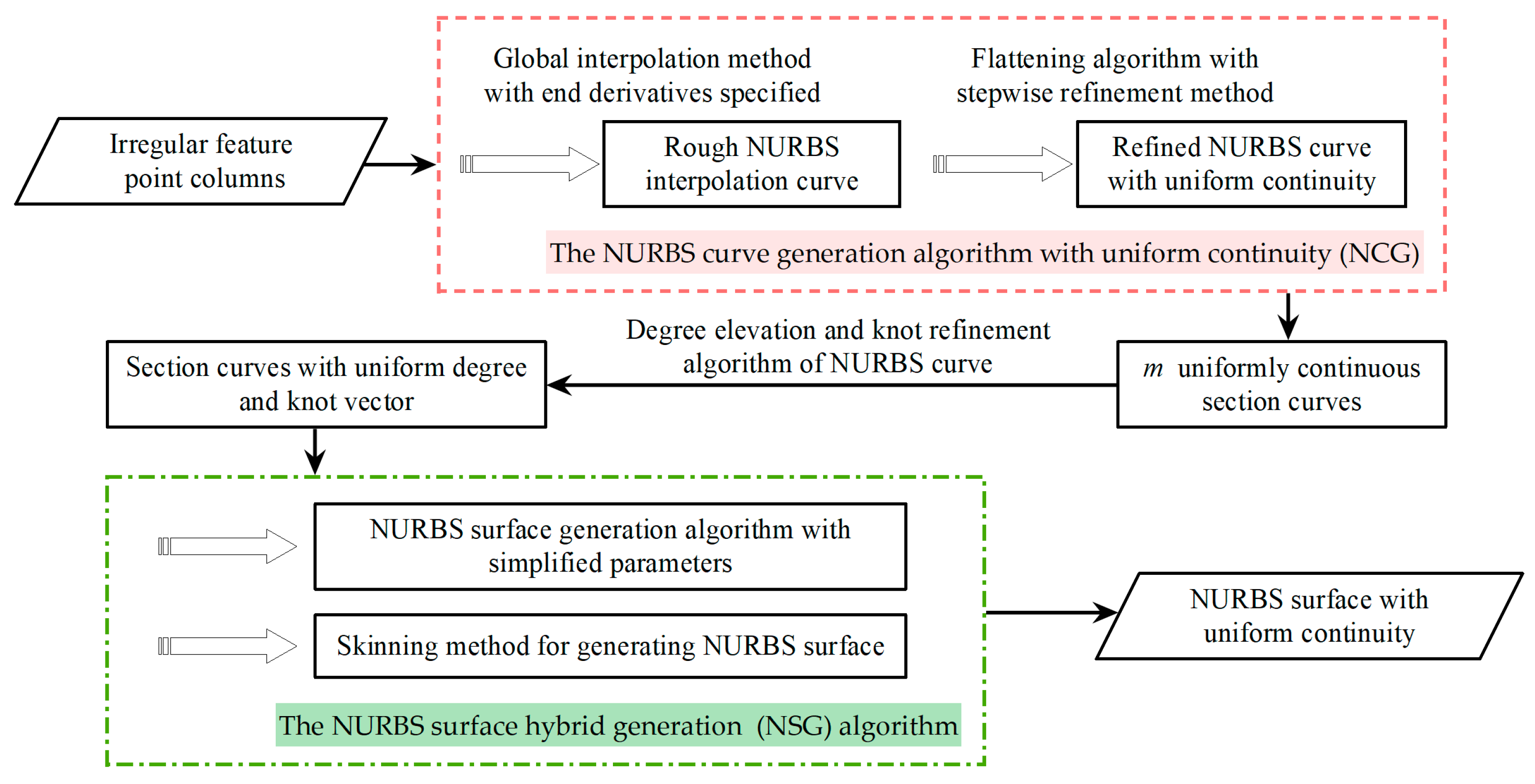
3.2. Rapid Reconstruction of NURBS Surface

In establishing curvature-continuous NURBS hull surface models through surface modeling techniques that permit unified mathematical representation, significant challenges arise in generating NURBS surfaces that simultaneously achieve high precision and computational efficiency. To address this, Zhu [40] proposed the fast NURBS surface generation (FNSG) model with uniform continuity specifically targeting hull surface modeling.

Figure 1 presents the flowchart of the FNSG model. The model employs the NURBS curve generation (NCG) algorithm with uniform continuity to produce NURBS curves with unified continuity and utilizes the NURBS surface hybrid generation (NSG) algorithm to adaptively simplify surface representation parameters. This integrated approach enhances generation efficiency while ensuring the objectives of unified mathematical representation and curvature continuity. Specific implementations of the NCG and NSG algorithms, along with associated parameters referenced in the FNSG model, are detailed in Ref. [40].

4. Methodology

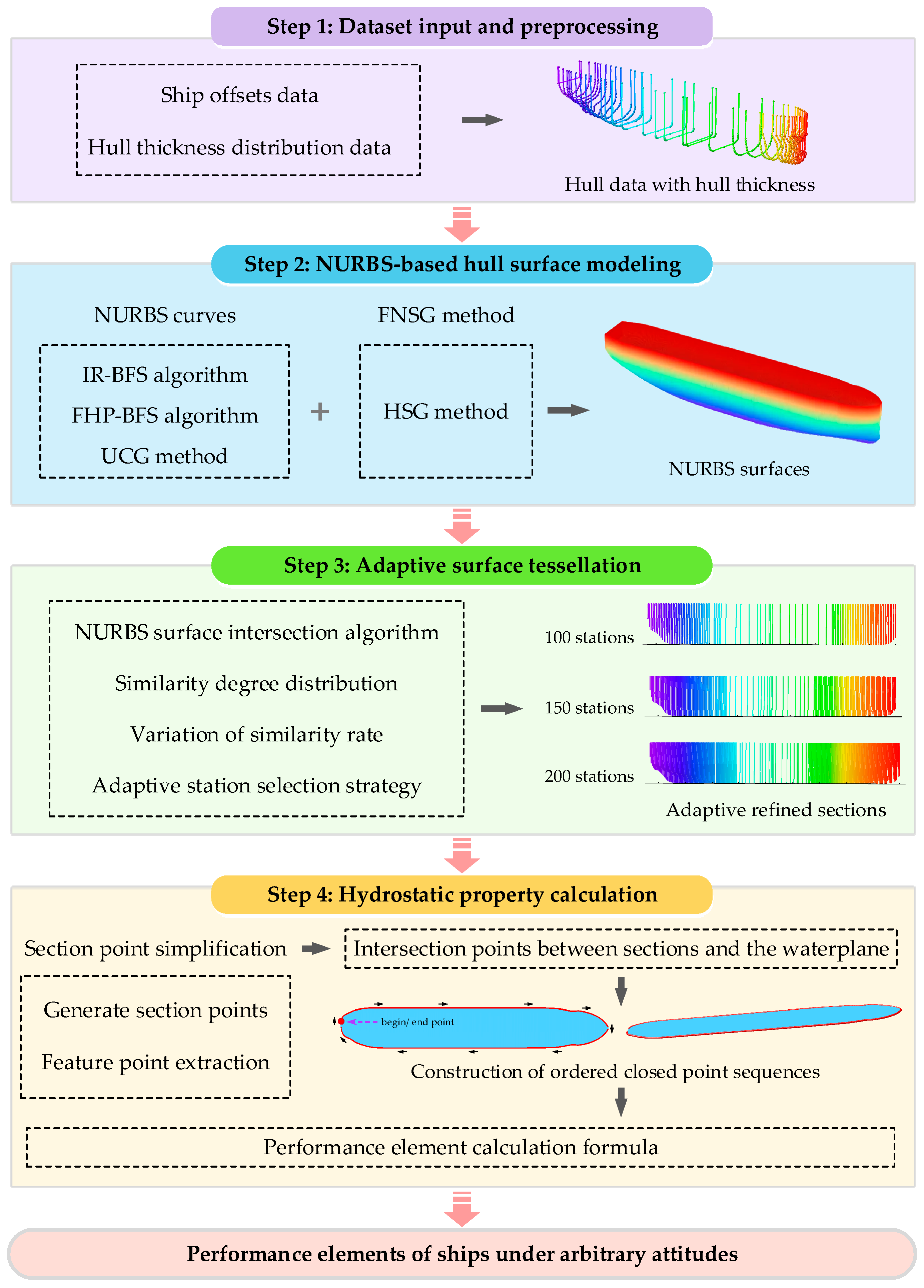
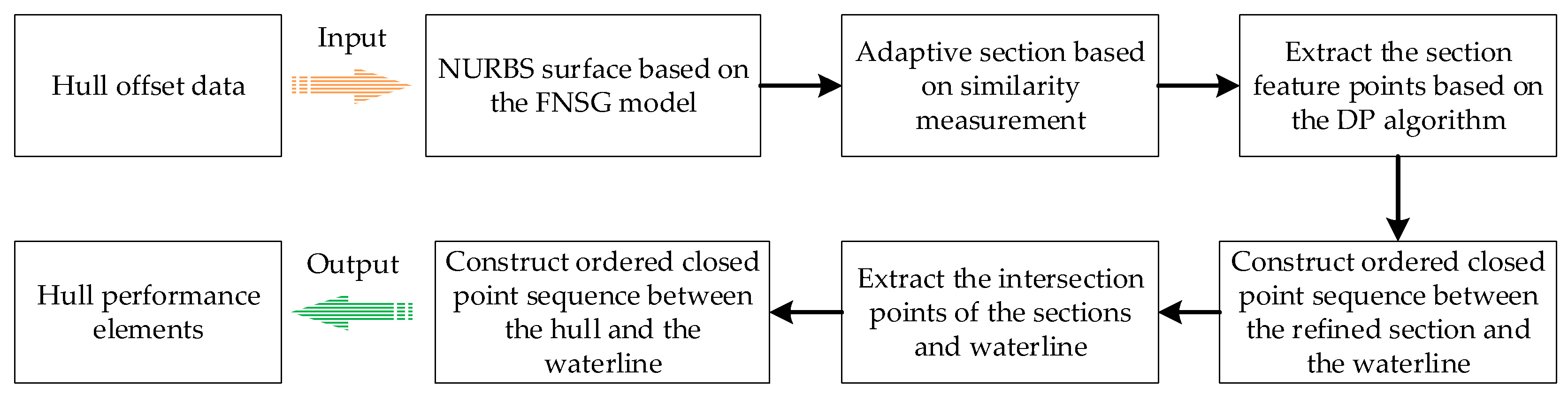
4.1. Framework of QB Method

The intricate motion responses of damaged ships in dead ship condition under severe conditions, where their attitudes frequently exceed conventional operational envelopes, render conventional models inadequate due to low computational efficiency and limited applicability when determining damaged stability parameters. To overcome these critical limitations, this section introduces the Quasi-Bonjean (QB) method for precise computation of ship performance elements under complex attitudes.

The QB method draws inspiration from the design concept of Bonjean curves: calculating hull performance parameters such as ship displacement and buoyancy center through a set of transverse sectional area curves at different waterlines. Although ingeniously designed, Bonjean curves are only applicable for determining submerged sectional areas under conventional trim conditions and cannot compute ship performance elements with heel angles or unconventional trim. To resolve this limitation, this study first constructed longitudinally distributed 3D hull cross-sections, simulated the ship condition at arbitrary attitudes by adjusting draft, heel angle, and trim angle parameters, and then calculated ship performance elements.

Figure 2 presents the QB method’s framework, structured into four sequential steps.

• Step 1: Dataset input and preprocessing: This step constructs hull surface data considering shell thickness based on the initial design offsets and shell thickness distribution.
• Step 2: NURBS-based hull surface modeling: This step constructs NURBS surface models based on the hull surface data.
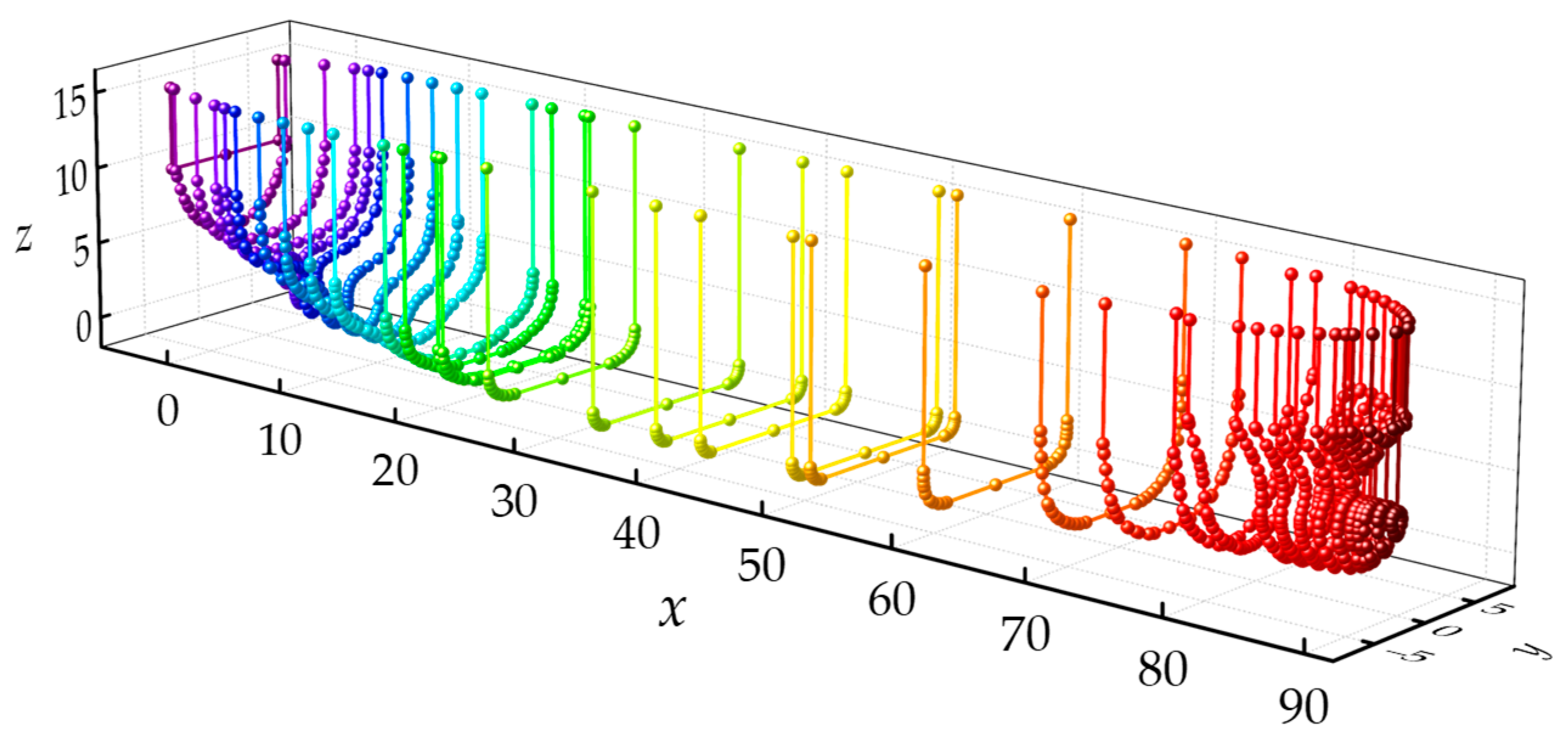
• Step 3: Adaptive Surface Tessellation (AST) method: This step generates multi-station sections via NURBS surface intersection algorithm and then applies adaptive refinement algorithm to create simplified sections that maximally preserve longitudinal distribution characteristics while minimizing section quantity.
• Step 4: Hydrostatic property calculation: This step calculates hull performance elements in arbitrary attitudes by constructing ordered closed point sequences of submerged hull geometry.

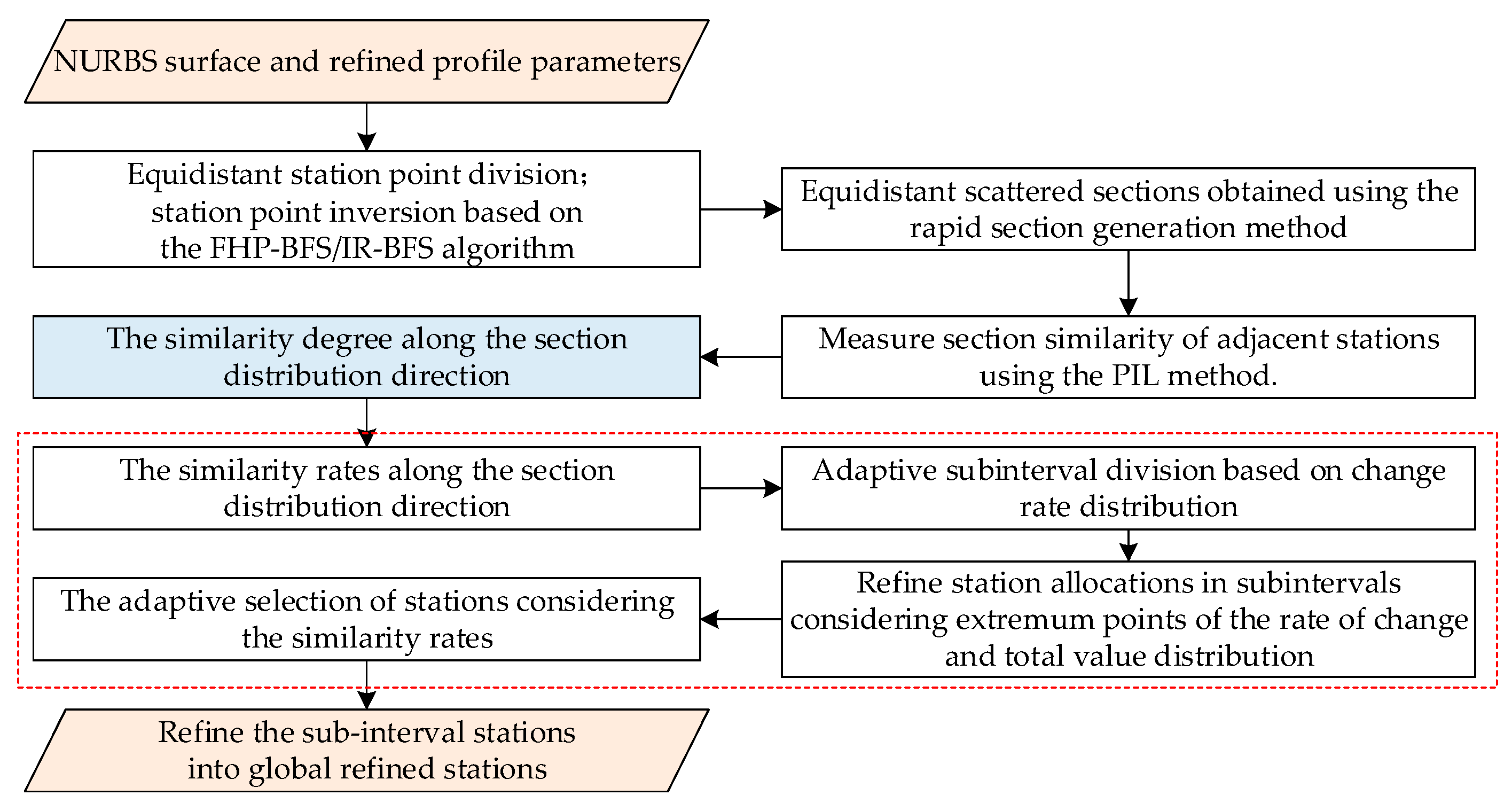
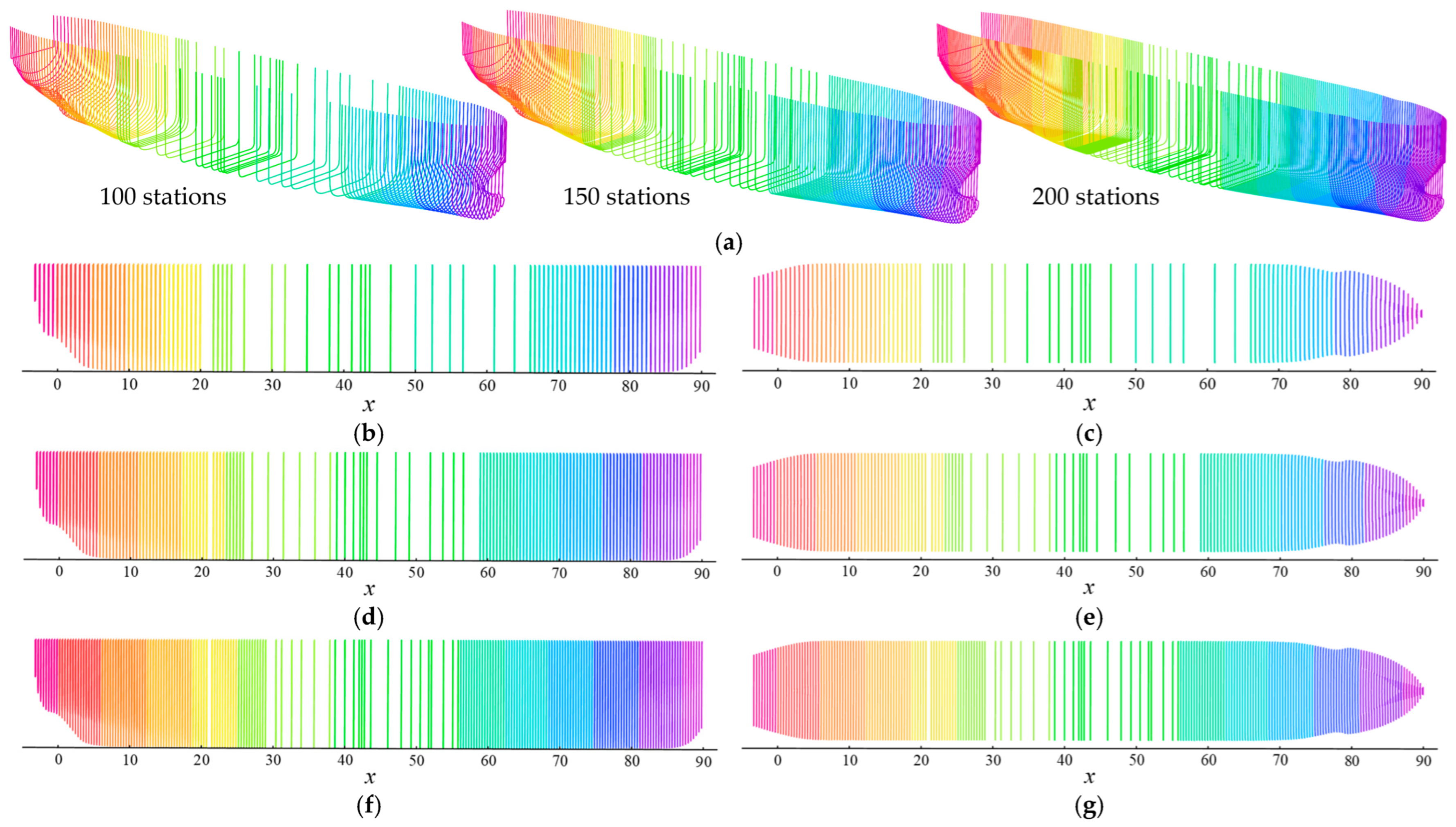
Figure 2. Framework of Quasi-Bonjean (QB) method.

Figure 2. Framework of Quasi-Bonjean (QB) method.

In step 1, hull section data (hull design offsets) exclude shell thickness considerations, while actual ship displacement calculations must account for thickness effects; therefore, the original sectional offsets require correction using shell thickness distribution data. This study employs polygon offset algorithm to determine thickness-expanded section data. As shown in Figure 3, black solid lines indicate original polygon, red dash-dotted lines indicate expanded polygon, green circular points indicate the original sectional offsets, and red triangular markers indicate expanded points (extension length L). Algorithm specifics are detailed in Ref. [70].

In step 2, the hull surface with unified continuity was generated using the FNSG algorithm. Specifically, the NCG method was used to generate NURBS-expressed hull sections by integrating IR-BFS and FHP-BFS algorithms; then, the NSG method was used to construct the hull NURBS surface based on the sectional curves.

In step 3, the transverse sections were firstly obtained by NURBS surface intersection algorithm; then, the similarity distribution curve was constructed along the ship length to identify simplified stations that preserve hull longitudinal characteristics. The AST method is detailed in Section 4.2.

In step 4, the refined NURBS sections were discretized into scattered points, with key feature points extracted to simplify profile representation; then, the sections were intersected with waterplanes at arbitrary attitudes to construct the submerged hull geometry; finally, the performance parameters were computed. The performance element calculation method is detailed in Section 4.3.

4.2. AST Method

To address the problem of rapidly, accurately, and adaptively describing hull surfaces through transverse sections, this study proposes the AST method. The concept of enhancing computational efficiency through adaptive approaches is analogous to the strategy of improving traffic flow efficiency via adaptive signal control systems in road transportation networks [71].

Figure 4 shows the flowchart of the AST method, which consists of two key processes: adaptive selection of refinement stations and adaptive generation of refined sections. The first process derives parametric refinement through section similarity distribution, analogous to the “training” phase in artificial neural networks. The second process produces optimized sections by integrating predefined refinement parameters with the obtained adaptive parameters, corresponding to the “generation” phase in artificial neural networks.

The AST method takes the hull NURBS surface generated by the FNSG model as input, proceeding through three computational phases: (1) discretizing the hull into boundary sections of surface patches, (2) quantifying the similarity distribution of sections along the longitudinal direction to obtain the similarity variation rate, and (3) generating refined cross-sections via the station-adaptive selection mechanism. Therefore, the adaptive station selection process fundamentally employs the section similarity measurement method coupled with the adaptive station selection strategy.

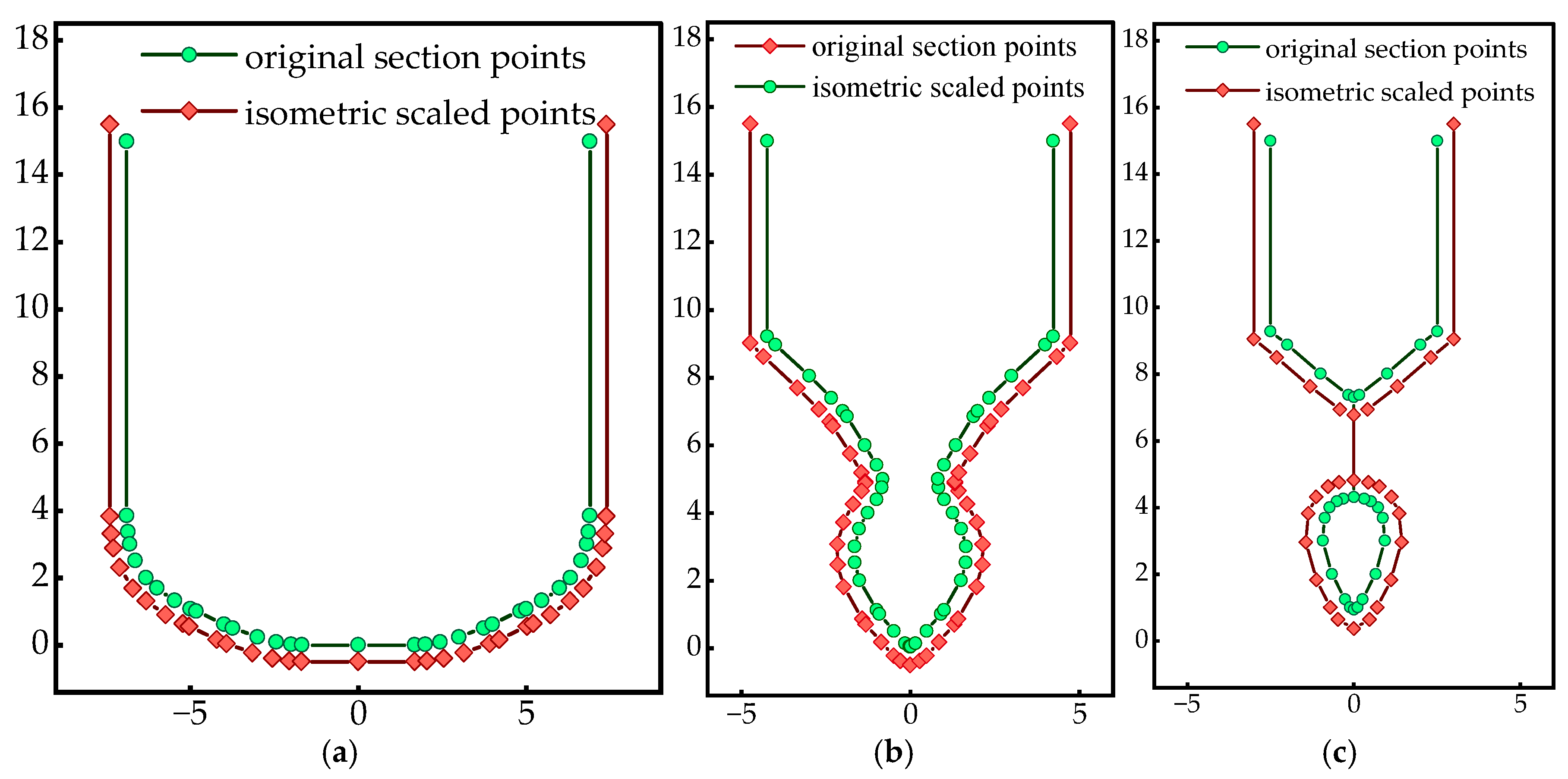
4.2.1. Selection of Similarity Measurement Elements

The transverse sections distributed along the longitudinal direction in three-dimensional space demonstrate that reducing section subdivision intervals yields approximately identical or even equivalent adjacent sections, while increasing intervals tend to produce sections with significant differences in both geometric shape and spatial orientation. Therefore, appropriate section distribution parameters must be considered when evaluating intersection similarity.

Figure 5 shows the effects of geometry variations and spatial distribution discrepancies of 3D sections on surface representation. Both Figure 5a,b display sections with equal spacing along the x-axis direction, denoted as Se1-Se3 and Se4-Se6, respectively. In Figure 5a, the three sections have identical shapes but different spatial positions, while in Figure 5b the three sections share the same central spatial positions but exhibit different shapes. Figure 5c and Figure 5d present the NURBS surfaces reconstructed from the sections in Figure 5a and Figure 5b, respectively, demonstrating distinct surface characteristics resulting from spatial distribution variations and geometric shape differences.

If spatial position variations are neglected during section similarity evaluation, the refined sections Se1 and Se3 of Figure 5c fail to accurately capture the nonlinear distribution characteristics of the surface along the x-axis, leading to significant errors in surface parameter calculations. Similarly, ignoring geometric shape variations would select refined sections Se4 and Se6 in Figure 5c, which cannot reproduce the original surface’s morphological features.

In conclusion, the evaluation of hull section similarity must simultaneously consider both the spatial distribution and geometric shape characteristics of sections in three-dimensional space, achieving the objective of precisely representing surface variation features using the minimum number of sections.

4.2.2. Similarity Measurement Method

This section introduces the Locality In-between Polylines (LIP) distance to evaluate similarity between two sections. The LIP algorithm, which was originally proposed for analyzing spatiotemporal trajectory similarity of moving objects, defines distance functions on 2D trajectory paths and calculates similarity through composite feature function values of inter-trajectory characteristics.

Figure 6 illustrates the LIP distance. Trajectories $P_m(m=1,2,\cdots ,a)$ and $Q_n(n=1,2,\cdots ,b)$ in two-dimensional space were formed by chronologically connecting discrete points into polygons, with intersection points labeled $I_1,I_2,$ $\cdots ,I_{i+1}$. The individual closed polygons formed are designated as ${\mathrm{polygon}}_1,\cdots ,$ ${\mathrm{polygon}}_i,$ ${\mathrm{polygon}}_{i+1}$, whose enclosed areas are $S_1,S_2,\cdots ,$ $S_i,S_{i+1}$, respectively. When the endpoints of polygons failed to intersect, their endpoints were connected to form closed regions, as demonstrated by segment $P_a{Q}_b$. The LIP distance between trajectories $P_m(m=1,2,\cdots ,a)$ and $Q_n(n=1,2,\cdots ,b)$ is defined by Equation (1).

$$\left\{\begin{array}{l}LIP(P,Q)={\displaystyle \sum _{\forall {\mathrm{polygon}}_j}{S}_j\cdot w_j}\\ w_i={\displaystyle \frac{{\mathrm{Length}}_P(I_j,I_{j+1})+{\mathrm{Length}}_Q(I_j,I_{j+1})}{{\mathrm{Length}}_P+{\mathrm{Length}}_Q}}\end{array}\right.$$

(1)

where $w_i$ denotes the weighting factor for each closed polygon ${\mathrm{polygon}}_i$, quantifying its contribution to the LIP distance between trajectories. ${\mathrm{Length}}_P$ and ${\mathrm{Length}}_Q$ represent the total lengths of polygons P and Q, respectively, while ${\mathrm{Length}}_P(I_j,I_{j+1})$ and ${\mathrm{Length}}_Q(I_j,I_{j+1})$ denote the lengths of polygons P and Q along segment $I_j,I_{j+1}$, respectively.

The evaluation of section similarity using LIP distance follows a relationship where larger LIP distance values indicate lower section similarity. This study adopts LIP measurement based on three technical justifications: (1) LIP integrates interactive area variations between adjacent sections; (2) LIP holistically evaluates spatial positioning and morphological changes; (3) characteristic point distribution patterns in hull sections exhibit topological equivalence with moving object trajectories, enabling mutual parametric conversion. Regarding the third justification, the 3D hull section data originated from intersection curves obtained by cutting NURBS surfaces with planes. This geometric property enables direct projection onto 2D yz-plane.

Figure 7 demonstrates the section similarity measurement of Figure 5. Figure 7a shows the sectional relationship between Se₁ and Se₂, forming two non-zero area regions S₁ and S₂. The total lengths of both sections correspond to the cumulative Euclidean distances of Se₁ and Se₂ polygonal vertices in 2D space. For non-zero area regions, the length represents the perimeters of closed Se₁/Se₂ polygons. Section similarity was calculated by Equation (1). The section similarity between Se₂ and Se₃ in Figure 7b can be analogously calculated. Sections Se₁ and Se₃ were symmetrically distributed about the plane containing Se₂. The intersecting closed regions between Se₂ and Se₃ exhibited equivalent enclosed areas and perimeters to those of Se₁ and Se₂, resulting in identical LIP distances. These confirm that LIP distances between sections depend on spatial relationships and geometric configurations but remain direction-independent of sections.

Figure 7c,d show Se₅Se₆ and Se₇Se₈ forming two closed regions with non-zero areas. Their area and weighting factor calculations follow identical methods to Figure 7a,b, but diverge in handling intersecting linear segments between sections. Duplicate segment endpoints are systematically organized to construct closed regions while preserving topological integrity. Zero-area closed regions exert null influence on section similarity metrics.

In conclusion, the LIP distance for section similarity evaluation achieves dual functionality: incorporating spatial distribution characteristics and geometric shape variations in hull sections while preserving computational simplicity in similarity quantification.

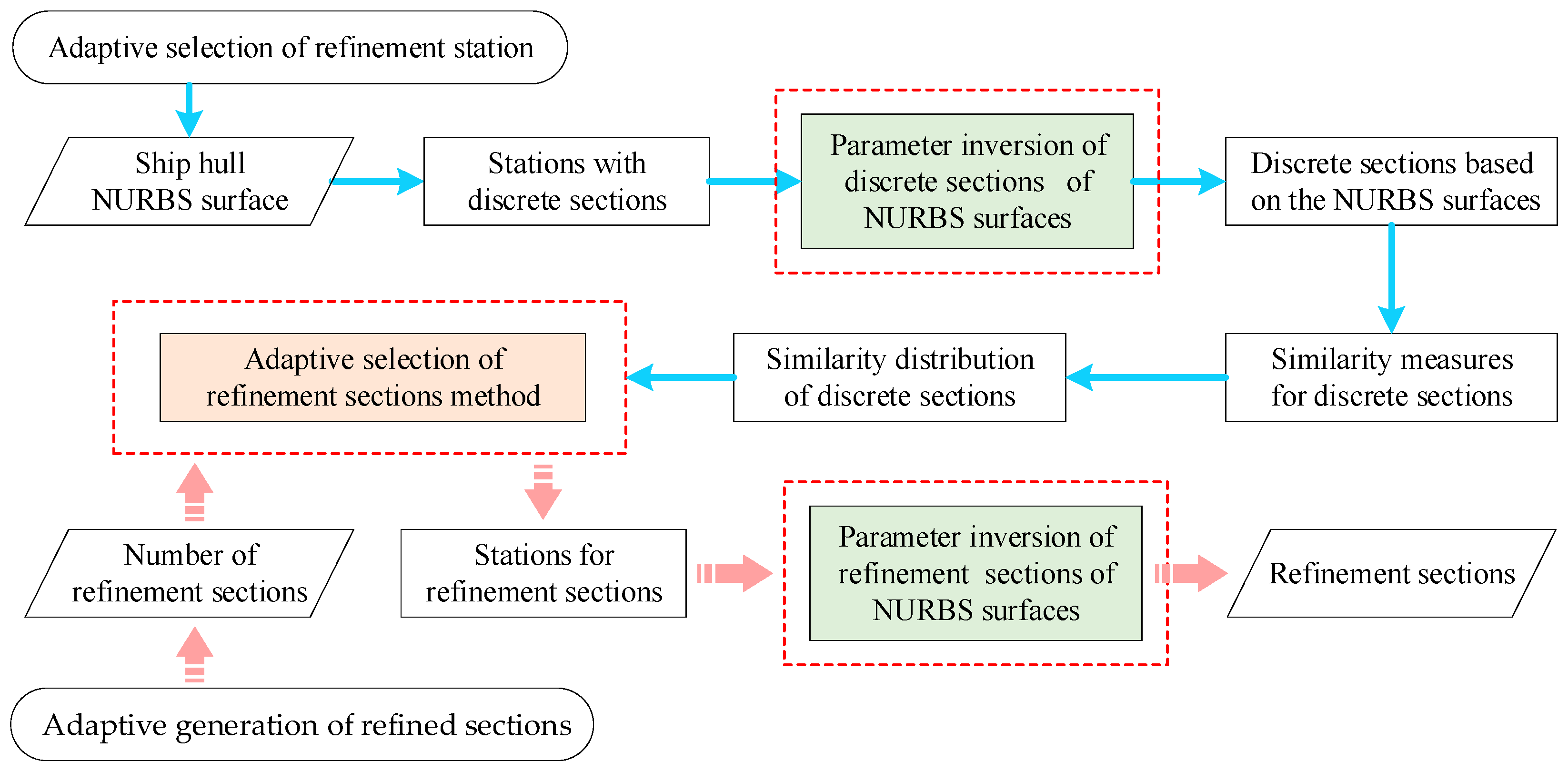
4.2.3. Adaptive Station Selection Strategy

The adaptive station selection strategy aims to generate stations that optimally express longitudinal hull characteristics based on section similarity distributions. As shown in Figure 8, the strategy begins with inputting the hull NURBS surface and refinement station count, followed by discretizing the NURBS surface into multiple sections. Subsequently, pairwise similarity measurements between sections were conducted to generate a similarity distribution curve, and finally, the stations matching the section similarity distribution were selected.

As sections of the first and last stations were mandatorily retained in the refined set, the similarity distribution curve was effectively computed from the second station onward relative to the first. During sampling quantity allocation, the process first constructed similarity variation rates and then adaptively partitioned sub-intervals based on sign changes in similarity variation rates. Given the total number of refined stations, specific sampling quantities per sub-interval were allocated according to both the numerical magnitudes and quantities of extrema points, ensuring that systematic distribution aligned with geometric evolution patterns. In addition, the extremum points are defined as stations where the similarity variation rate simultaneously exceeds or is lower than that of both their preceding and subsequent stations. The allocation formula is defined by Equation (2).

$$n_i=(w_V\cdot {\displaystyle \frac{V_i}{{\displaystyle \sum _i{V}_i}}}+w_N\cdot {\displaystyle \frac{N_i}{{\displaystyle \sum _i{N}_i}}})\cdot m, i=1,2,\cdots$$

(2)

where $n_i$ denotes the sampling count of the $i-th$ subinterval; $m$ represents the total refined station count; $V_i$ and $N_i$ denote the quantity of extrema points; $w_V$ and $w_N$ denote the weighting coefficients of $V_i$ and $N_i$.

The station selection process mandatorily incorporates both terminal stations and sub-interval boundary stations. The strategy prioritizes extrema points of similarity variation rates, selecting candidates in descending order of absolute values. Two scenarios typically emerge: (1) incomplete selection of extrema points within sub-intervals (indicating fulfilled sampling quota) and (2) sub-intervals containing fewer extrema points than required sampling numbers (indicating insufficient variation features). For the latter case, the total area enclosed by the similarity curve and coordinate axis is proportionally divided into equal-area regions corresponding to remaining sampling quotas, with regional endpoints automatically designated as supplementary refined stations.

The sampling strategy systematically subdivides intervals through similarity variation rates, explicitly accounting for regional geometric diversity (particularly in bow and stern regions) by evaluating similarity rates. Additionally, it prioritizes extrema-point ordering within sub-intervals, incorporating critical features through preferential selection of sections with lower overall similarity. Finally, the equal-area regions method addresses cumulative variations caused by repeated similarity increments. These mechanisms collectively ensure uniform distribution of refined sections across hull regions, enabling the adaptive station selection strategy to achieve robust performance even when handling complex geometric variations with multi-scale similarity transitions.

4.3. Performance Elements Calculation Method

Figure 9 illustrates the computational flowchart for performance elements. The algorithm adaptively generated sections conforming to the hull’s longitudinal characteristics by the SAT method and then extracted feature points from section points through the Douglas–Peucker (DP) algorithm. For each section, it constructed ordered closed point sequences below the waterplane while systematically organizing intersection points between sections and waterlines into coherent polylines defining the hull–waterplane interface. Final performance elements were calculated by hydrostatic method.

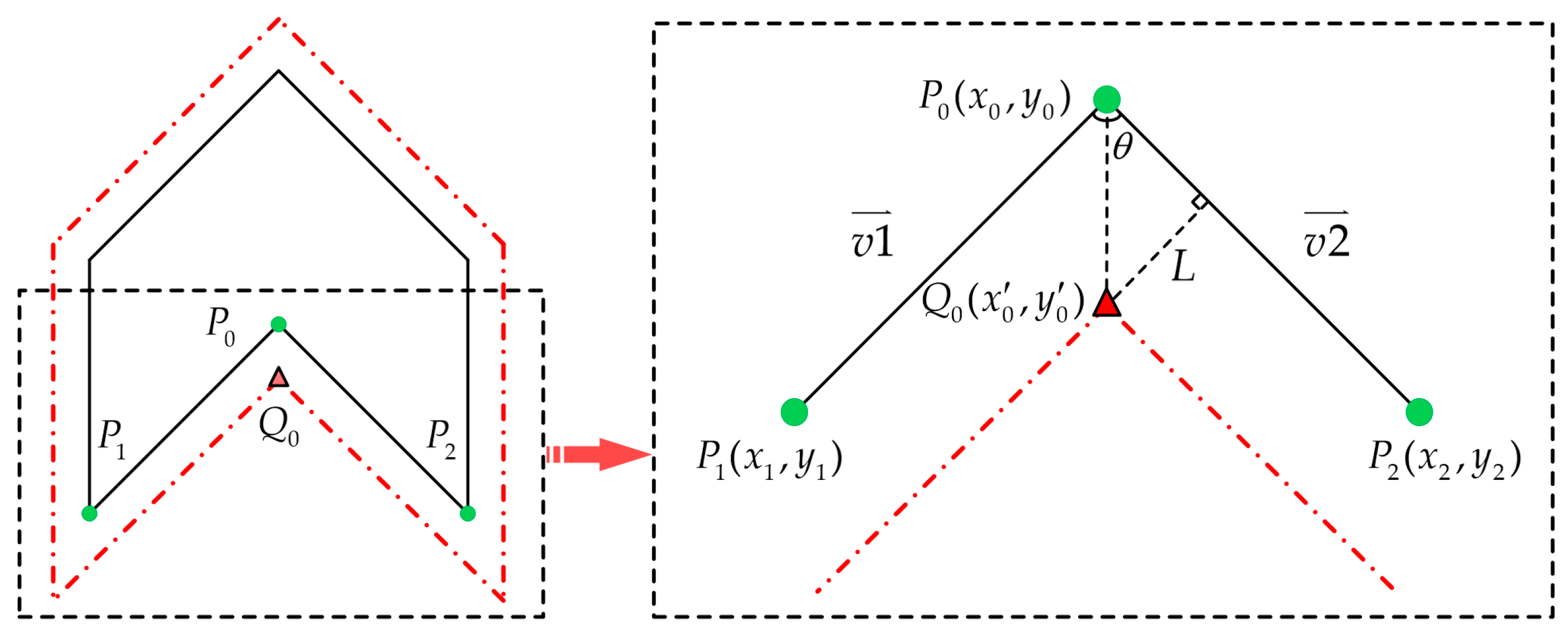
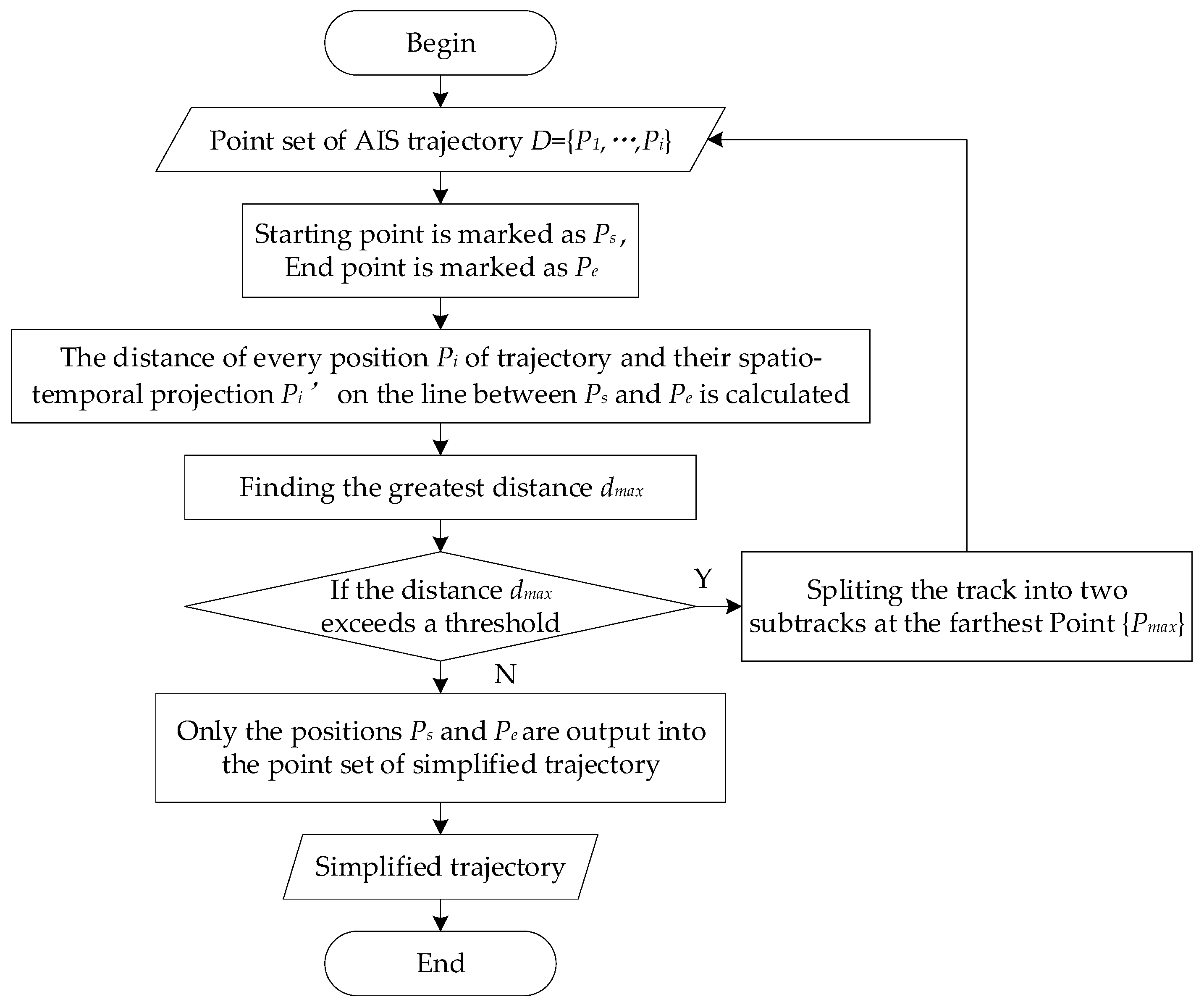
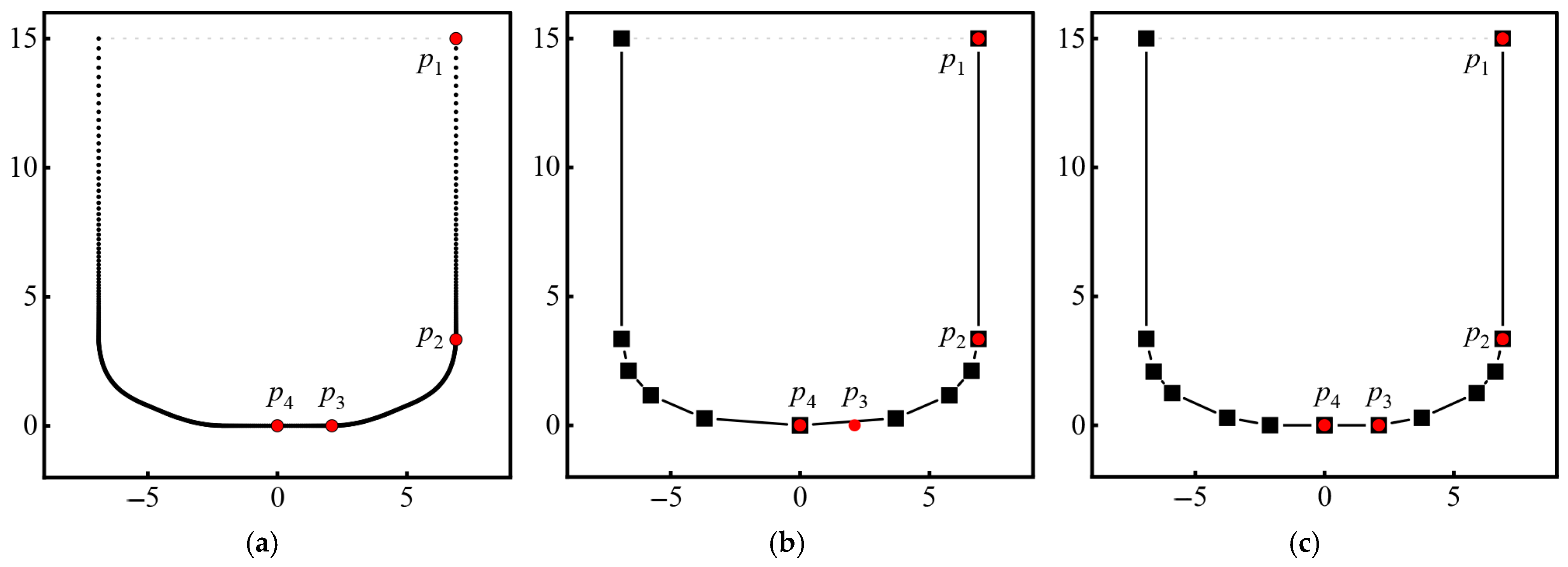
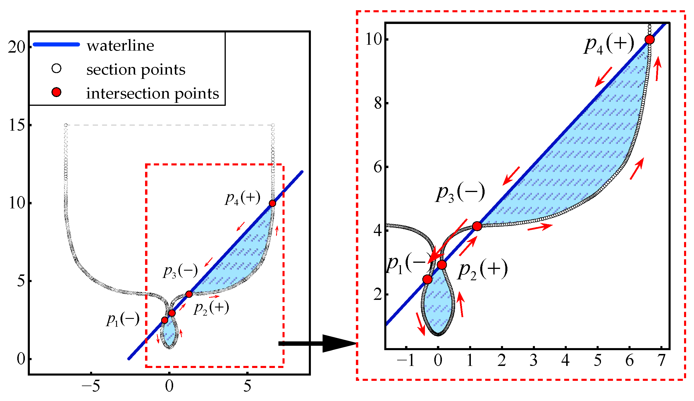
4.3.1. Extraction Algorithm of Section Feature Points

This section introduces the DP algorithm for extracting key feature points. As shown in Figure 10, the DP algorithm recursively simplifies linear points using a threshold-controlled approach. Widely used in trajectory simplification for moving objects due to its efficiency and topological fidelity, the algorithm is also applicable to spatially ordered coordinates without temporal dependencies. Thus, it effectively reduces dimensionality while preserving geometric fidelity and extracting key feature points. For more details, refer to Ref. [72].

Hull surfaces combine linear segments and curved sections, requiring separate DP algorithm processing for optimal feature point simplification. Figure 11a shows the original 600-point scatter distribution of a hull section, with black circles as discrete points, red circles as landmark points, $p_1{p}_2/p_3{p}_4$ as linear segments, and $p_2{p}_3$ as a curved section. Figure 11b illustrates unified DP simplification (ε = 0.2 m), resulting in 11 points but eliminating critical point $p_3$, violating geometric constraints. In contrast, Figure 11c uses independent processing (linear and curved sections handled independently under ε = 0.2 m), generating 13 points that preserve straight edges and curvature transitions. This analysis confirms that independent simplification better aligns with the section’s hybrid geometry.

4.3.2. Fast Intersection Judgment Method

Conventional intersection calculation organizes section feature points into linear segments and assesses potential intersections iteratively. However, testing all segments exhaustively reduces computational efficiency. This study introduces an accelerated method using spatial coherence and geometric prioritization for faster section–waterplane intersections.

Figure 12a shows the relationship between a section line and waterplane. Here, $O$ is the coordinate origin, $\theta$ indicates the angle between the waterplane and the section, and $p_1\sim p_4$ are selected feature points. This study proposes a coordinate transformation method to accelerate intersection interval detection in three steps: translating the origin to the waterplane–z axis intersection, rotating the system by $\theta$ degrees, and monitoring z-value changes in sequential feature points to identify intersection interval.

Figure 12b illustrates the mechanism for rapid intersection interval detection, with point $O^{\prime }$ as the new origin and points $p_1^{\prime }\sim p_4^{\prime }$ as section features. The new coordinate system $y^{\prime }{O}^{\prime }{z}^{\prime }$ was rotated counterclockwise by angle $\theta$ relative to $yOz$. The transformation formula of $p_1^{\prime }\sim p_4^{\prime }$ is defined in Equation (3).

$$\left\{\begin{array}{l}{y}_i^{\prime }=(y_i-\Delta y)\cdot \cos \theta +(z_i-\Delta z)\cdot \sin \theta \\ z_i^{\prime }=(z_i-\Delta z)\cdot \cos \theta -(y_i-\Delta y)\cdot \sin \theta \end{array}\right.\hspace{1em}i=1,2,\cdots$$

(3)

where $\begin{array}{cc}\Delta y=y_o^{\prime }-y_o,& \Delta z=z_o^{\prime }-z_o\end{array}$. After obtaining $p_1^{\prime }\sim p_4^{\prime }$, the intersection intervals can be determined by judging the positive and negative variations in the $z^{\prime }$-axis between consecutive feature points. If adjacent points have opposite polarities in components $z_1^{\prime }>0$ (point $p_1^{\prime }$) and $z_2^{\prime }<0$ (point $p_2^{\prime }$), segment $p_1^{\prime }{p}_2^{\prime }$ contains an intersection. A direct intersection occurs if $z_i^{\prime }=0$. After determining the interval, exact intersection coordinates in system $y^{\prime }{O}^{\prime }{z}^{\prime }$ were solved using linear equations and then transformed to system $yOz$ via Equation (4).

$$\left\{\begin{array}{l}{y}_i=y_i^{\prime }\cdot \cos \theta -{z^{\prime }}_i\cdot \sin \theta +\Delta y\\ z_i=z_i^{\prime }\cdot \cos \theta +{y^{\prime }}_i\cdot \sin \theta +\Delta z\end{array}\right.\hspace{1em}i=1,2,\cdots$$

(4)

In conclusion, the proposed method quickly determines the intersection interval, avoids ineffective intersections between section line segments and waterlines, and significantly improves computational efficiency.

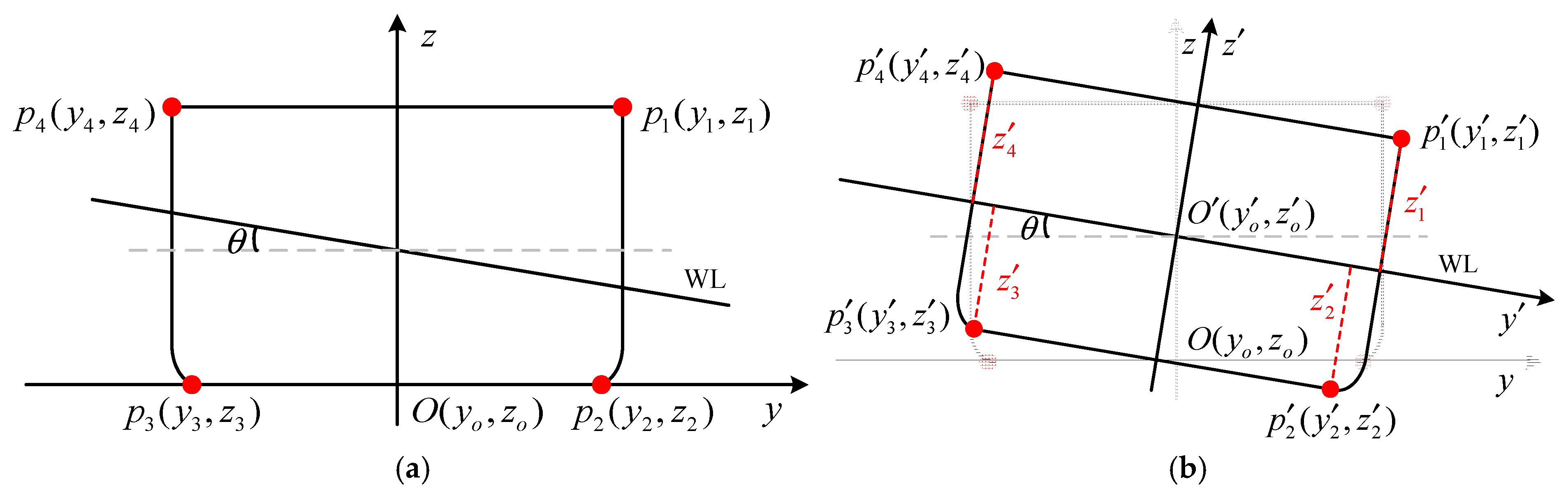
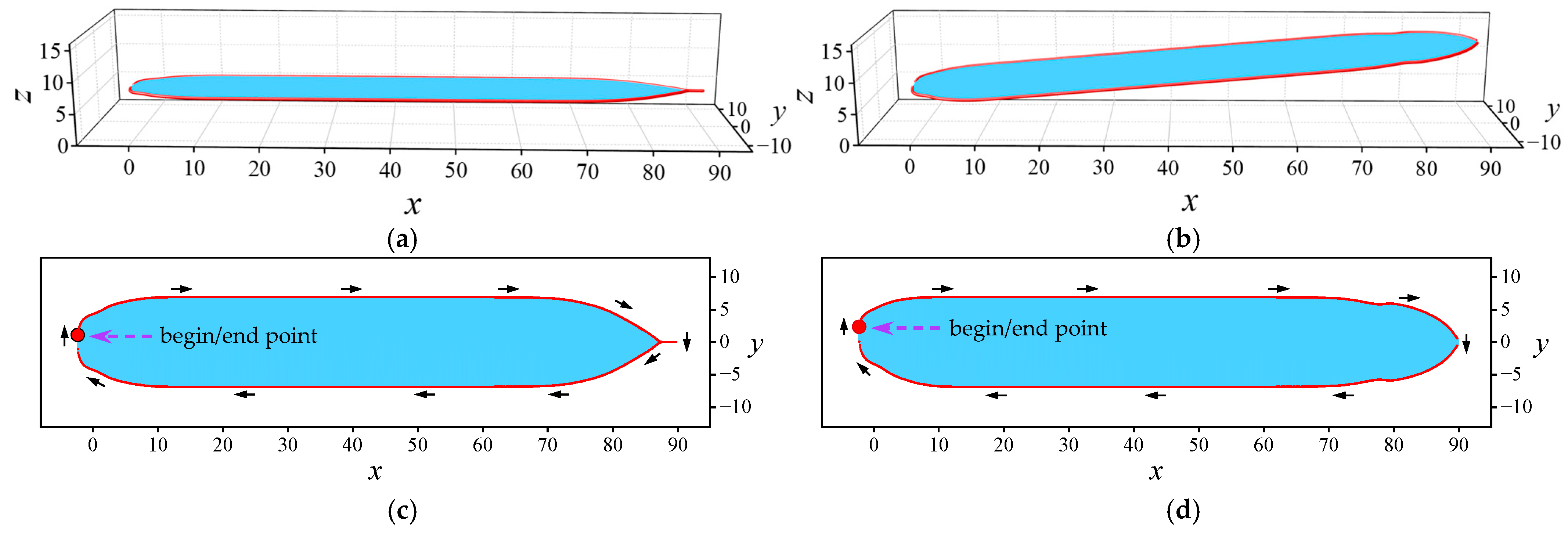
4.3.3. Construction of Ordered Closed Point Sequence

Damaged ship equilibrium analysis requires determining hull performance elements (displacement, buoyancy center) and waterplane characteristics (area, moments of inertia). Performance elements can be calculated by integrating submerged section elements along the ship length. Waterplane parameters were derived from closed sequences formed by ordered intersection points. This study proposes the methodology for generating these ordered point sequences, which is essential for accurate damaged stability calculations.

Figure 13 shows the construction of multi-intersection ordered closed point sequences between hull sections and waterplanes. With four intersection points $p_1~p_4$, the algorithm processed section points counterclockwise to identify intervals. For intersection $p_i(i=1,2,\cdots )$, if the left adjacent point’s z > 0 and right adjacent z < 0, mark $p_i(-)$ as the start of a sub-interval; if left z < 0 and right z > 0, mark $p_i(+)$ as the end. Sub-intervals connect sequentially by linking termination point $p_i(+)$ to the next initiation $p_i(-)$, then close the contour by reverse-linking waterplane intersections. Special cases: (1) For boundary-left intersections (point $p_i$, z = 0), mark $p_i(+)$ if the right point’s z > 0 or $p_i(-)$ if z < 0. (2) When consecutive intersections enclose only waterplane-on points, construct linear sub-intervals.

Closed point sequence construction starts by creating an initial loop through clockwise connectivity of port/starboard intersection points based on the station sequence, forming closed contours for dual-intersection sections. For sections with more than two intersections, iterative application generates multiple closed contours. Figure 14a,c show ordered waterplane contours at a 6 m even-keel draught, computed using 400 random stations for clarity. Figure 14b,d demonstrate the algorithm’s universal applicability under arbitrary floating conditions, showing closed contours at 6 m draught with combined heel (15°) and trim (3°).

5. Results and Discussions

This chapter validates the effectiveness of the AST and QB methods against the International Association of Classification Societies (IACS) accuracy standards, utilizing hydrostatic data from the chemical tanker “MV-Z” as benchmark references.

5.1. Datasets and Setting

5.1.1. Dataset Introduction

The chemical tanker “MV-Z” contains 35 stations of offset data, with

Table 1. Offset points of chemical vessel “MV-Z” without plate thickness.

x (the 8th Station)			x (the 8th Station)			x (the 28th Station)
Index	y	z	Index	y	z	Index	y	z
1	0.000	0.000	1	0.000	0.000	1	0.000	0.000
2	0.240	0.000	2	5.977	0.000	2	0.000	0.035
3	0.471	0.035	3	6.000	0.000	3	0.034	0.155
4	0.734	0.118	4	6.283	0.051	…	…	…
…	…	…	5	6.476	0.142	13	2.012	3.000
22	6.691	5.532	6	6.636	0.272	14	2.000	3.188
23	6.788	6.000	7	6.802	0.500	…	…	…
24	6.868	6.902	8	6.874	0.694	25	4.000	8.432
25	6.900	7.578	9	6.900	0.934	26	4.721	9.194
26	6.900	15.000	10	6.900	15.000	27	4.721	15.000

presenting partial section points that exclude hull shell plate thickness. The principal dimensions are as follows: length between perpendiculars (Lpp) = 86.70 m, molded breadth (B) = 13.80 m, and shell plate thickness = 12 mm.

5.1.2. Tolerance Criteria

The IACS specifies stability calculation tolerance as follows: “Programs utilizing hull geometry models for stability computations shall permit output deviations when benchmarked against either approved stability documentation or classification society-endorsed reference models.” The tolerance quantification methodology is defined in Equation (5):

$$D={\displaystyle \frac{V_b-V_c}{V_b}}\times 100\%$$

(5)

where $D$ represents percentage tolerance, $V_b$ denotes reference values, and $V_c$ indicates computed values. Additionally, the reference value must come from approved stability documentation or classification society-certified models.

Experimental validation compares calculated elements with ship hydrostatic tables.

Table 2. The tolerance thresholds of the relevant quantities of ship shape specified by IACS.

Elements	Acceptable Tolerance 1	Acceptable Tolerance 2
DISP	2%	-
LCB	1%	50 cm
VCB	1%	5 cm
LCF	1%	50 cm
MTC	2%	-
KMT	1%	5 cm
KML	1%	50 cm

specifies tolerance thresholds for hull geometry-dependent quantities. If both tolerance 1 and tolerance 2 apply, the acceptable deviation is the larger of the two.

5.1.3. Dataset Preprocessing

Figure 15 shows section offset points with shell thickness compensation using the PIS algorithm, exaggerated by a 0.5 m expansion for visual clarity. Station 11 (aft-midship) and Stations 29/32 (forward sections to bulbous bow) illustrate geometric evolution characteristics. The figure shows that the original section features are accurately retained through one-to-one correspondence between the values before and after expansion.

Figure 16 presents expanded 3D station points of 35 stations. Figure 17 shows the hull NURBS surface including deck plane and transom surfaces, which are generated through identical parameterization as the hull surface.

5.2. Analysis of Experimental Process

This section systematically examines the adaptive section generation process, the distribution of longitudinal sections, and their correlations with hull characteristics, thereby assessing the operational workflow of the AST method.

Figure 18 presents 400 uniformly discretized NURBS surface sections along the longitudinal axis. The smooth chromatic transition across stations in Figure 18a confirms the reliable performance of the inversion algorithms and the validity of the section generation methodology. In Figure 18b, the bow concavity geometry is clearly resolved, illustrating that the section discretization density adequately captures the hull characteristics.

Figure 19 illustrates the distribution of section similarity degree across 400 refined stations. In the interval $x\le 10$, the decreasing trend of elevated similarity degree signifies progressively increasing section similarity. In the interval $10<x\le 70$, the stable similarity degree clustered around zero confirms consistently high section similarity. In the interval $70<x\le 80$, an initial increase in similarity degree followed by a decrease reflects transitional similarity reduction and subsequent recovery. In the interval $x>80$, consistent similarity degree growth indicates sustained similarity enhancement. The bow and stern intervals exhibit greater similarity degree variability compared to midship regions, confirming reduced section similarity at bow and stern and suggesting the need for increased sampling density of characteristic sections.

To accurately assess hull section similarity, this study investigates the distribution patterns of section similarity by calculating the continuous variation rate of similarity between adjacent sections. Figure 20 illustrates the longitudinal distribution of section similarity variation rates along the hull, which corresponds to the trends in similarity values: higher variation rates in the bow and stern regions, and lower similarity and variation rates at the midship. In the interval x ≤ 5, the variation rate gradually decreases to 0, indicating stabilized section geometry. In the interval 5 < x ≤ 70, the variation rate remains close to 0, confirming consistent spatial and geometric characteristics. In the interval 70 < x ≤ 80, the increasing variation rate reflects geometric modifications. In the interval x > 80, the variation rate decreases sharply, suggesting rapid geometric evolution. Uniform sampling across all intervals would overlook features in areas with low similarity and variation rates, such as the midship section. Therefore, refined sub-intervals are defined based on similarity variation patterns, allowing for the adaptive selection of characteristic sections in different variation rate intervals to precisely capture hull geometric features.

The dotted-dashed lines in Figure 20 delineate adaptive sampling intervals partitioned by sign changes in the variation rates of adjacent section similarity. In the interval x ≤ 5, two complete sampling intervals are identified: one capturing significant similarity variations at the stern that gradually diminish to zero and another transitioning to increased variation rates due to the influence of the sternpost’s lower edge. Similarly, in the interval x > 70, two intervals are defined to resolve the bow concavity region (70 < x ≤ 80) and its transition into the bulbous bow formation. This interval division method effectively identifies hull section characteristics along the longitudinal axis, accurately reflecting actual spatial–geometric variations. Adaptive station refinement is subsequently achieved through three criteria: extrema of similarity degree, variation rates of similarity, and cumulative similarity degree.

Figure 21a illustrates sections refined using the AST method with 100, 150, and 200 stations. The 100-station refinement features denser sections in the bow and stern to precisely capture complex geometric details, whereas fewer sections are allocated to the midship region (10 ≤ x ≤ 70) due to its relatively uniform shape. Figure 21b highlights the refined sections’ ability to resolve smooth transitional details between the stern (x < 10) and bow (x > 80) regions. Figure 21c explicitly reconstructs the concavity formation process within the critical interval of the bow (70 < x < 80), thereby confirming geometric fidelity in high-curvature regions.

The adaptive 150-station refinement shows an increase in section density in both the bow/stern and midship regions compared to the 100-station refinement. Specifically, the bow/stern areas exhibit higher density increment, which is crucial for accurately resolving critical geometric features such as sternpost transitions and bulbous bow contours. A comparison of Figure 21b,d indicates density growth in the midship intervals of 20 < x < 30 and 50 < x < 60, while minimal changes are observed in the interval 30 < x < 50. This can be attributed to the high similarity within the interval 30 < x < 50, which permits sparse sampling. The bow and stern regions (x < 20, x > 60) exhibit tighter section spacing, effectively capturing critical sternpost–bulbous transition features. Additionally, Figure 21c,e demonstrate an increase in density in the bow concavity regions (70 < x < 80), thereby enhancing the accuracy of hydrodynamic calculations.

The 200-station refinement enhances the resolution of bow and stern details significantly compared to the 150-station model while preserving the sampling efficiency at midship. Analysis of Figure 21d,f reveals that the interval 30 < x < 50 experiences only a minor increase in density, despite its high similarity, which underscores the algorithm’s prioritization of low-similarity regions. The midship intervals of 20 < x < 30 and 50 < x < 60 gain substantially more sections, respectively. In the bow and stern regions (x < 20 and x > 60), tighter spacing is achieved, improving the articulation of the sternpost and bulbous bow. Lastly, Figure 21e,g illustrate an increase in density within the bow concavity (70 < x < 80) and the bulbous bow region (x > 80).

In conclusion, the AST method adaptively generates sections that are optimally aligned with the longitudinal characteristics of the hull, thereby reducing the number of redundant sections compared to uniform sampling. Its high sensitivity to three-dimensional spatial positioning and variations in shape similarity rates allows for the precise resolution of complex distribution patterns in the bow and stern regions while minimizing oversampling in lower-similarity areas such as the midship.

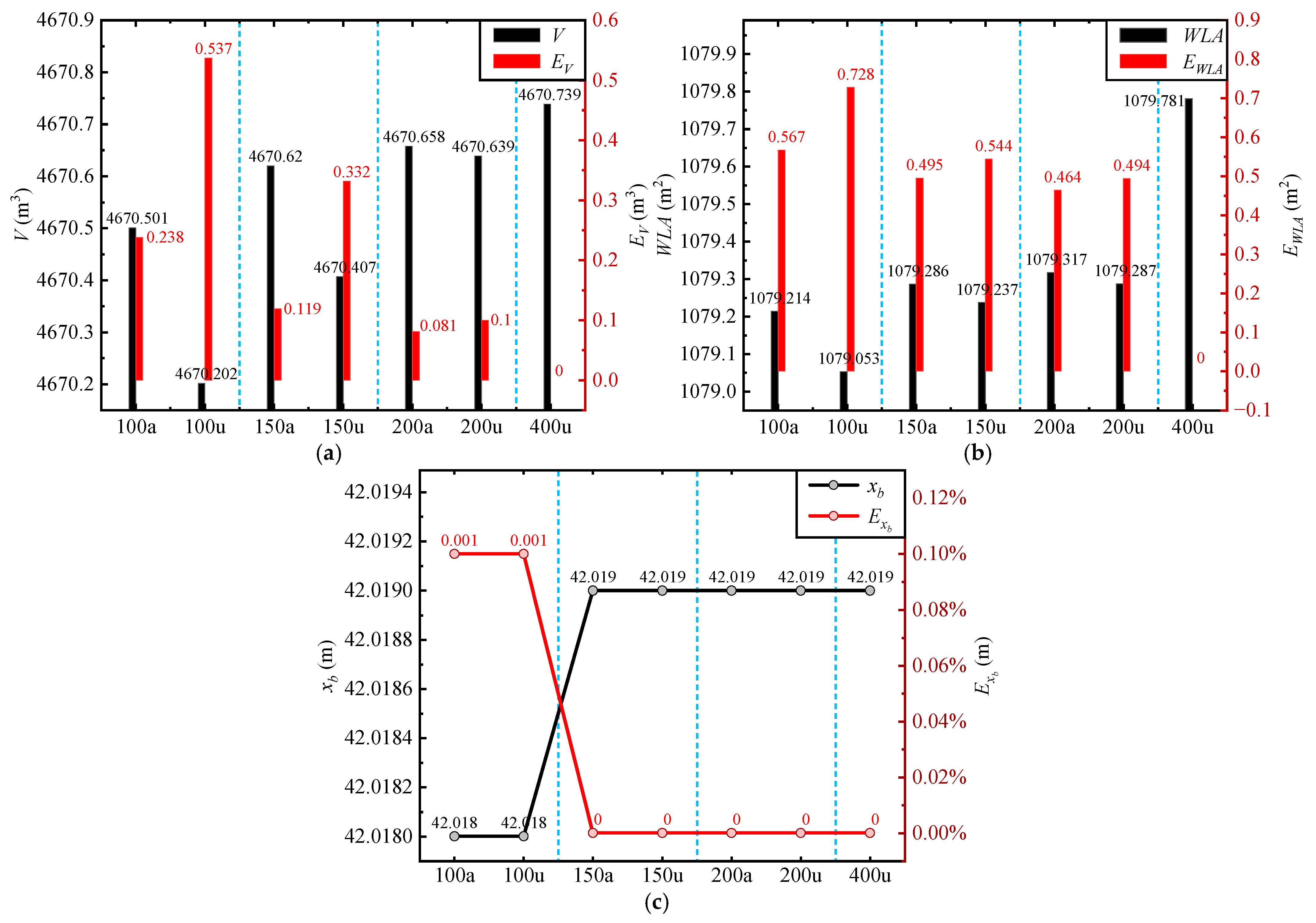
5.3. Validation of AST Method Accuracy

This section evaluates the effectiveness of refined sections in representing hull NURBS surface accuracy through performance element calculations. The experiment compares adaptive refinement (as shown in Figure 21) with uniform refinement at varying station densities (100, 150, and 200 stations), using three key metrics: displacement volume, waterplane area, and longitudinal center of buoyancy (LCB). A uniformly refined model with 400 stations serves as the reference benchmark, since hydrostatic calculation precision generally increases with higher section density.

Figure 22 presents the comparisons of calculated elements between adaptive refinement (denoted as 100a/150a/200a) and uniform refinement (denoted as 100u/150u/200u). The analysis is conducted under a 5 m even-keel condition and evaluates the displacement volume (V) with absolute error (E_V), waterplane area (WLA) with error (E_WLA), and the longitudinal center of buoyancy (x_b) with error (E_xb). The errors are quantified as the absolute deviations from the baseline established by the 400-station uniform refinement.

Figure 22a illustrates the comparison of displacement volume error (E_V) between adaptive and uniform refinement methods. Specifically, adaptive refinements with 100/150/200 stations yield E_V values of 0.238/0.119/0.081 m³, respectively, while uniform refinements result in E_V values of 0.573/0.332/0.100 m³ for the same station counts. A detailed comparative analysis indicates that the error of adaptive 100-station refinement (100a, E_V = 0.238 m³) is lower than that of uniform 150-station refinement (150u, E_V = 0.332 m³), but it remains higher than the error of uniform 200-station refinement (200u, E_V = 0.100 m³). These results confirm the substantial accuracy enhancement achieved by employing adaptive section sampling in E_V calculations.

Figure 22b presents the comparison of the waterplane area error (E_WLA). The adaptive refinement method with 100/150/200 stations achieves errors of 0.567/0.495/0.464 m², respectively, while the uniform refinement method yields errors of 0.728/0.544/0.494 m² for the same station counts. Specifically, the adaptive refinement with 100 stations (100a, 0.567 m²) outperforms the uniform refinement counterpart with the same number of stations (100u, 0.728 m²). However, it exhibits a slightly higher error compared to the uniform refinement with 150 stations (150u, 0.544 m²). Notably, the adaptive refinement with 150 stations (150a, 0.495 m²) surpasses the precision of uniform refinement at 150 stations (150u, 0.544 m²) and closely matches the accuracy achieved by uniform refinement at 200 stations (200u, 0.494 m²). These findings demonstrate the effectiveness of adaptive refinement in minimizing errors for waterplane area calculations.

Figure 22c assesses the accuracy of longitudinal center of buoyancy (LCB) calculations, where both adaptive and uniform refinement methods yield identical errors: E_xb = 0.001 m at 100 stations and zero error (E_xb = 0.000 m) at 150 and 200 stations. This equivalence indicates that both methods achieve the same level of LCB precision, attaining zero-error accuracy when refined to 150 stations.

The experimental results conclusively demonstrate that the adaptive sections generated by the AST method not only improve the accuracy of hydrostatic calculations but also accurately reflect the characteristics of the hull NURBS surface. Furthermore, comparative validation highlights the superiority of the AST method: it achieves equivalent precision with fewer sections than those required for uniform refinement while preserving parametric fidelity.

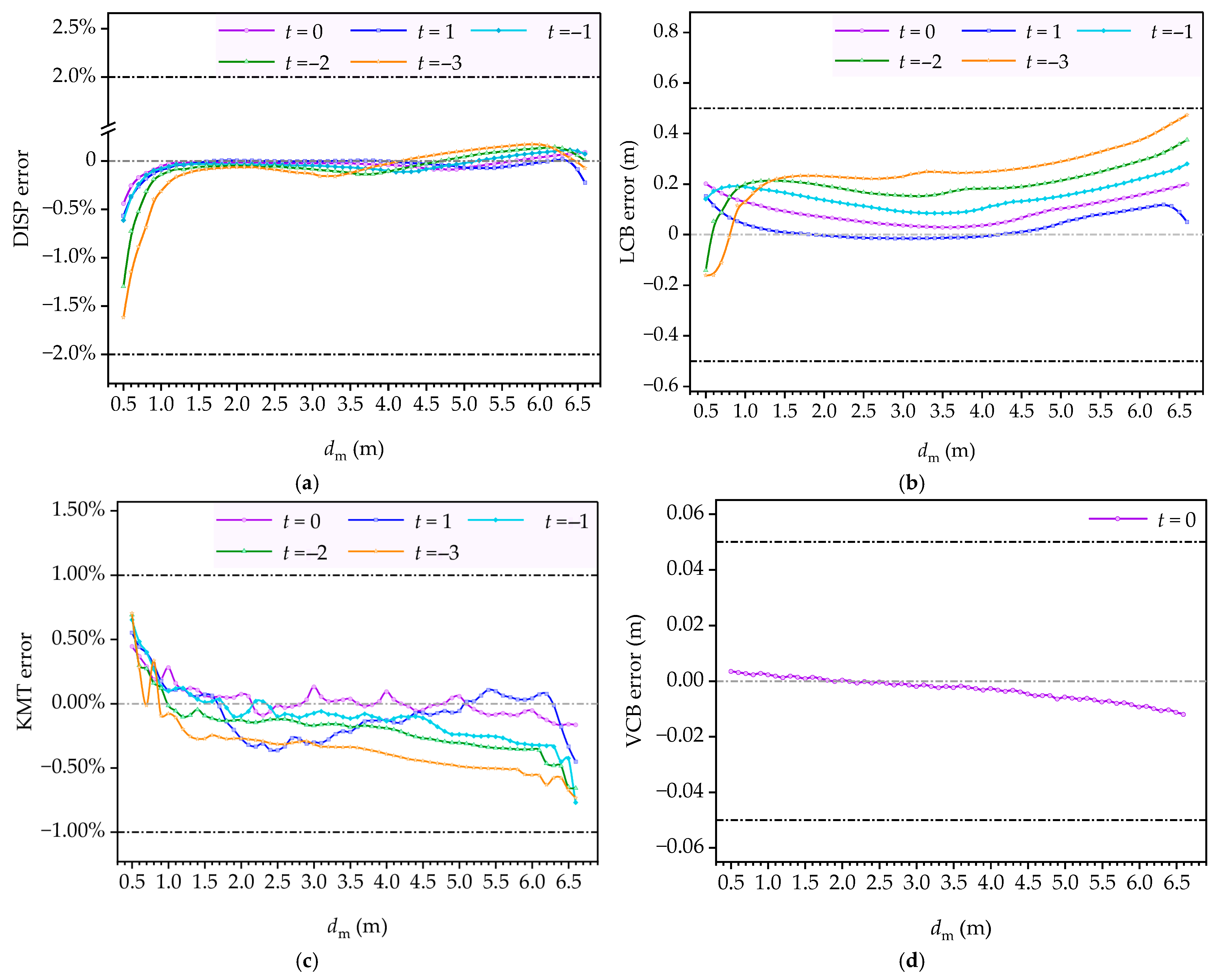
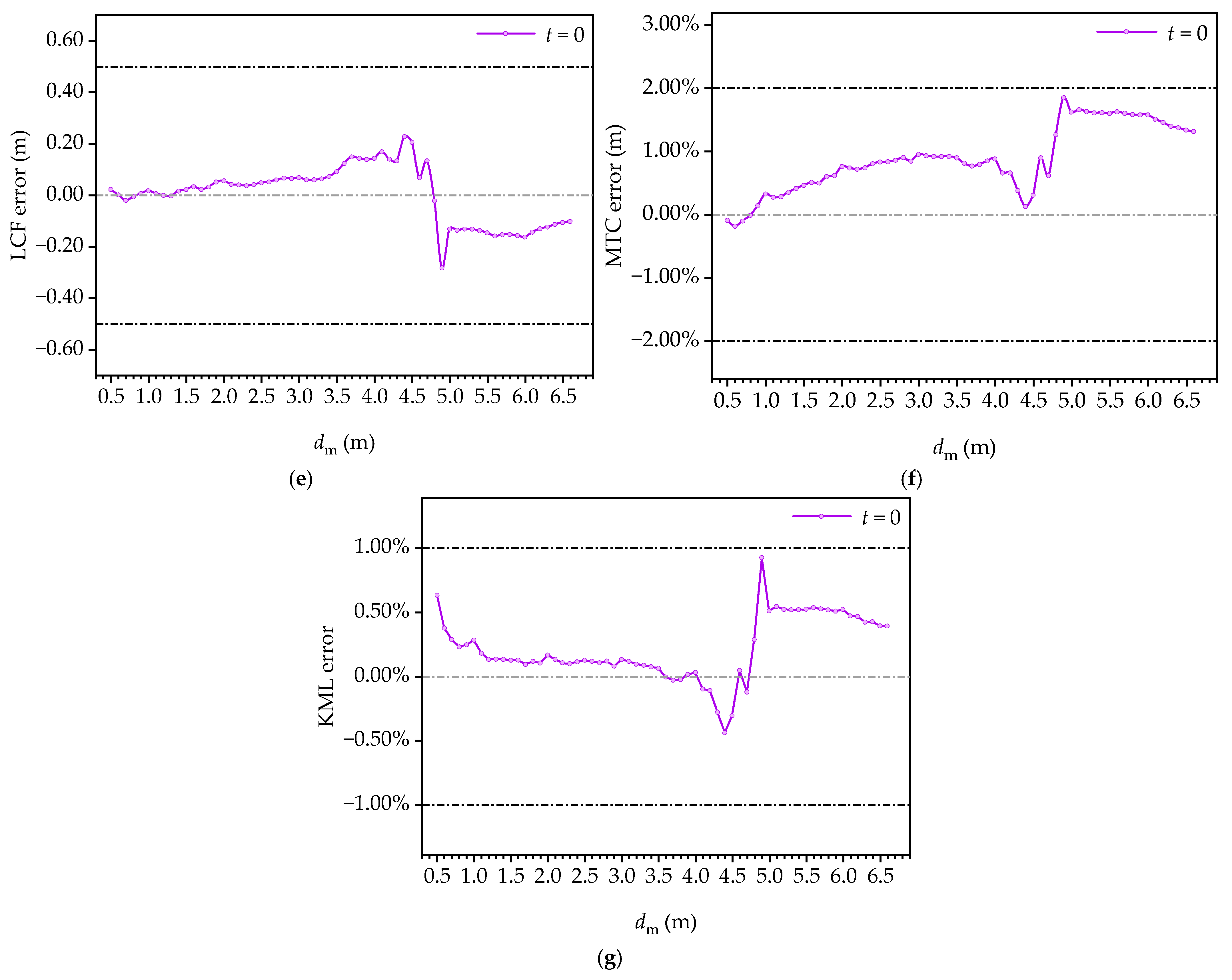
5.4. Validation of QB Method Accuracy

This section verifies the effectiveness of the QB method in calculating performance parameters, using IACS-regulated error thresholds as criteria and hydrostatic table data as benchmarks.

The experiment evaluates seven hydrodynamic parameters under upright conditions (DISP, LCB, KMT, VCB, LCF, MTC, KML) and three parameters under pure trim variations (DISP, LCB, KMT), all derived from hydrostatic tables.

To demonstrate the generalizability of the method, computational errors are systematically analyzed across all loading conditions. Seawater density is dynamically determined by the DISP/∇ ratio based on matching entries in the hydrostatic tables. In addition, the numerical results are systematically presented in Appendix A 

Table A1. Calculation error of displacement in upright ($\theta =0, t=0$). Where, t denotes trim; V_b denotes reference values from hydrostatic table; V_c denotes computed values.

dm	DISP (Vb)	DISP (Vc)	Error	dm	DISP (Vb)	DISP (Vc)	Error	dm	DISP (Vb)	DISP (Vc)	Error
0.5	365.3	366.908	−0.440%	2.6	2294.7	2295.246	−0.024%	4.7	4493.7	4497.521	−0.085%
0.6	445.7	446.838	−0.255%	2.7	2395.0	2395.581	−0.024%	4.8	4603.2	4607.233	−0.088%
0.7	527.9	528.804	−0.171%	2.8	2495.8	2496.439	−0.026%	4.9	4713.5	4717.638	−0.088%
0.8	611.7	612.469	−0.126%	2.9	2597.1	2597.698	−0.023%	5.0	4825.0	4828.588	−0.074%
…	…	…	…	…	…	…	…	…	…	…	…
2.2	1899.5	1899.722	−0.012%	4.3	4061.5	4063.734	−0.055%	6.3	6313.4	6309.220	0.066%
2.3	1997.4	1997.768	−0.018%	4.4	4168.7	4171.433	−0.066%	6.4	6430.3	6425.556	0.074%
2.4	2095.9	2096.317	−0.020%	4.5	4276.4	4279.661	−0.076%	6.5	6547.5	6542.175	0.081%
2.5	2195.0	2195.450	−0.021%	4.6	4384.5	4388.353	−0.088%	6.6	6664.9	6658.961	0.089%

,

Table A2. Calculation error of displacement in trim ($\theta =0,t=1$).

dm	DISP (Vb)	DISP (Vc)	Error	Tm	DISP (Vb)	DISP (Vc)	Error	dm	DISP (Vb)	DISP (Vc)	Error
0.5	387.3	389.505	−0.569%	2.6	2314.8	2314.915	−0.005%	4.7	4482.3	4484.127	−0.041%
0.6	467.6	469.316	−0.367%	2.7	2414.3	2414.376	−0.003%	4.8	4589.8	4591.958	−0.047%
0.7	549.9	551.338	−0.262%	2.8	2514.2	2514.282	−0.003%	4.9	4697.9	4700.433	−0.054%
0.8	634.0	635.148	−0.181%	2.9	2614.5	2614.512	0.000%	5.0	4806.2	4809.447	−0.068%
…	…	…	…	…	…	…	…	…	…	…	…
2.2	1922.2	1922.118	0.004%	4.3	4057.0	4057.792	−0.020%	6.3	6278.1	6276.946	0.018%
2.3	2019.6	2019.600	0.000%	4.4	4162.6	4163.611	−0.024%	6.4	6392.9	6393.054	−0.002%
2.4	2117.5	2117.505	0.000%	4.5	4268.8	4269.982	−0.028%	6.5	6504.0	6509.496	−0.085%
2.5	2215.9	2215.916	−0.001%	4.6	4375.2	4376.819	−0.037%	6.6	6611.3	6626.156	−0.225%

,

Table A3. Calculation error of displacement in trim ($\theta =0,t=-1$).

dm	DISP (Vb)	DISP (Vc)	Error	Tm	DISP (Vb)	DISP (Vc)	Error	dm	DISP (Vb)	DISP (Vc)	Error
0.5	363.3	365.539	−0.616%	2.6	2282.7	2283.683	−0.043%	4.7	4519.4	4521.932	−0.056%
0.6	441.9	443.526	−0.368%	2.7	2383.6	2384.688	−0.046%	4.8	4632.0	4634.029	−0.044%
0.7	522.6	523.855	−0.240%	2.8	2485.1	2486.301	−0.048%	4.9	4744.9	4746.446	−0.033%
0.8	605.2	606.085	−0.146%	2.9	2587.2	2588.406	−0.047%	5.0	4858.0	4859.107	−0.023%
…	…	…	…	…	…	…	…	…	…	…	…
2.2	1885.7	1886.343	−0.034%	4.3	4072.8	4077.289	−0.110%	6.3	6355.0	6348.059	0.109%
2.3	1983.9	1984.710	−0.041%	4.4	4183.3	4187.685	−0.105%	6.4	6471.9	6464.483	0.115%
2.4	2082.8	2083.671	−0.042%	4.5	4295.0	4298.691	−0.086%	6.5	6588.0	6581.138	0.104%
2.5	2182.5	2183.303	−0.037%	4.6	4407.0	4410.137	−0.071%	6.6	6702.7	6697.916	0.071%

,

Table A4. Calculation error of displacement in trim ($\theta =0,t=-2$).

dm	DISP (Vb)	DISP (Vc)	Error	dm	DISP (Vb)	DISP (Vc)	Error	dm	DISP (Vb)	DISP (Vc)	Error
0.5	388.7	393.746	−1.298%	2.6	2280.7	2282.111	−0.062%	4.7	4553.4	4553.314	0.002%
0.6	461.1	464.468	−0.730%	2.7	2382.0	2383.645	−0.069%	4.8	4667.8	4667.028	0.017%
0.7	536.7	539.514	−0.524%	2.8	2484.1	2485.899	−0.072%	4.9	4782.4	4781.060	0.028%
0.8	616.0	617.933	−0.314%	2.9	2586.7	2588.752	−0.079%	5.0	4897.3	4895.267	0.042%
…	…	…	…	…	…	…	…	…	…	…	…
2.2	1882.8	1883.778	−0.052%	4.3	4098.9	4101.364	−0.060%	6.3	6400.5	6392.061	0.132%
2.3	1981.0	1982.226	−0.062%	4.4	4212.0	4213.785	−0.042%	6.4	6515.1	6508.494	0.101%
2.4	2080.1	2081.379	−0.062%	4.5	4325.4	4326.661	−0.029%	6.5	6629.0	6625.132	0.058%
2.5	2180.1	2181.315	−0.056%	4.6	4439.2	4439.854	−0.015%	6.6	6742.3	6741.884	0.006%

,

Table A5. Calculation error of displacement in trim ($\theta =0,t=-3$).

dm	DISP (Vb)	DISP (Vc)	Error	dm	DISP (Vb)	DISP (Vc)	Error	dm	DISP (Vb)	DISP (Vc)	Error
0.5	443.9	451.088	−1.619%	2.6	2290.5	2292.795	−0.100%	4.7	4593.2	4589.837	0.073%
0.6	509.6	515.439	−1.146%	2.7	2392.1	2394.771	−0.112%	4.8	4708.5	4704.474	0.086%
0.7	578.7	583.845	−0.889%	2.8	2494.6	2497.616	−0.121%	4.9	4824.0	4819.412	0.095%
0.8	651.4	655.891	−0.689%	2.9	2598.0	2601.222	−0.124%	5.0	4939.6	4934.508	0.103%
…	…	…	…	…	…	…	…	…	…	…	…
2.2	1892.9	1894.077	−0.062%	4.3	4134.8	4133.911	0.022%	6.3	6445.4	6440.173	0.081%
2.3	1991.0	1992.413	−0.071%	4.4	4249.0	4247.382	0.038%	6.4	6558.6	6556.677	0.029%
2.4	2089.9	2091.593	−0.081%	4.5	4363.4	4361.267	0.049%	6.5	6672.6	6673.327	−0.011%
2.5	2189.8	2191.693	−0.086%	4.6	4478.2	4475.434	0.062%	6.6	6785.0	6790.015	−0.074%

,

Table A6. Calculation error of LCB in upright ($\theta =0,t=0$).

dm	LCB (Vb)	LCB (Vc)	Error	dm	LCB (Vb)	LCB (Vc)	Error	dm	LCB (Vb)	LCB (Vc)	Error
0.5	1.196	0.994	0.202	2.6	1.559	1.511	0.048	4.7	0.922	0.840	0.082
0.6	1.223	1.041	0.182	2.7	1.551	1.507	0.044	4.8	0.866	0.774	0.092
0.7	1.249	1.085	0.164	2.8	1.542	1.500	0.042	4.9	0.805	0.705	0.100
0.8	1.276	1.127	0.149	2.9	1.530	1.491	0.039	5.0	0.738	0.635	0.103
…	…	…	…	…	…	…	…	…	…	…	…
2.2	1.562	1.500	0.062	4.3	1.126	1.077	0.049	6.3	−0.067	−0.244	0.177
2.3	1.565	1.507	0.058	4.4	1.079	1.022	0.057	6.4	−0.118	−0.303	0.185
2.4	1.566	1.511	0.055	4.5	1.030	0.964	0.066	6.5	−0.167	−0.359	0.192
2.5	1.563	1.513	0.051	4.6	0.980	0.903	0.077	6.6	−0.215	−0.414	0.199

,

Table A7. Calculation error of LCB in trim ($\theta =0,t=1$).

dm	LCB (Vb)	LCB (Vc)	Error	dm	LCB (Vb)	LCB (Vc)	Error	dm	LCB (Vb)	LCB (Vc)	Error
0.5	9.214	9.061	0.153	2.6	3.765	3.779	−0.014	4.7	2.322	2.301	0.021
0.6	8.215	8.099	0.116	2.7	3.693	3.707	−0.014	4.8	2.254	2.227	0.027
0.7	7.465	7.377	0.088	2.8	3.623	3.637	−0.014	4.9	2.187	2.152	0.035
0.8	6.884	6.816	0.068	2.9	3.553	3.568	−0.015	5.0	2.122	2.076	0.046
…	…	…	…	…	…	…	…	…	…	…	…
2.2	4.080	4.088	−0.008	4.3	2.596	2.593	0.003	6.3	1.196	1.077	0.119
2.3	3.996	4.006	−0.010	4.4	2.527	2.520	0.007	6.4	1.120	1.007	0.114
2.4	3.916	3.927	−0.011	4.5	2.458	2.447	0.011	6.5	1.027	0.938	0.089
2.5	3.839	3.852	−0.013	4.6	2.390	2.374	0.016	6.6	0.921	0.871	0.051

,

Table A8. Calculation error of LCB in trim ($\theta =0,t=-1$).

dm	LCB (Vb)	LCB (Vc)	Error	dm	LCB (Vb)	LCB (Vc)	Error	dm	LCB (Vb)	LCB (Vc)	Error
0.5	−6.967	−7.108	0.141	2.6	−0.717	−0.825	0.108	4.7	−0.599	−0.738	0.139
0.6	−5.860	−6.033	0.173	2.7	−0.661	−0.765	0.104	4.8	−0.645	−0.788	0.143
0.7	−5.026	−5.212	0.186	2.8	−0.611	−0.710	0.099	4.9	−0.693	−0.840	0.147
0.8	−4.371	−4.562	0.191	2.9	−0.568	−0.663	0.095	5.0	−0.742	−0.894	0.152
…	…	…	…	…	…	…	…	…	…	…	…
2.2	−1.020	−1.147	0.127	4.3	−0.449	−0.574	0.125	6.3	−1.321	−1.566	0.245
2.3	−0.932	−1.053	0.121	4.4	−0.478	−0.609	0.131	6.4	−1.357	−1.610	0.253
2.4	−0.852	−0.969	0.117	4.5	−0.516	−0.648	0.132	6.5	−1.388	−1.653	0.265
2.5	−0.780	−0.893	0.113	4.6	−0.556	−0.691	0.135	6.6	−1.414	−1.694	0.280

,

Table A9. Calculation error of LCB in trim ($\theta =0,t=-2$).

dm	LCB (Vb)	LCB (Vc)	Error	dm	LCB (Vb)	LCB (Vc)	Error	dm	LCB (Vb)	LCB (Vc)	Error
0.5	−12.765	−12.623	−0.142	2.6	−3.031	−3.194	0.163	4.7	−2.224	−2.422	0.198
0.6	−11.457	−11.509	0.052	2.7	−2.914	−3.075	0.161	4.8	−2.240	−2.443	0.203
0.7	−10.392	−10.480	0.088	2.8	−2.808	−2.966	0.158	4.9	−2.257	−2.465	0.208
0.8	−9.401	−9.550	0.149	2.9	−2.711	−2.867	0.156	5.0	−2.275	−2.489	0.214
…	…	…	…	…	…	…	…	…	…	…	…
2.2	−3.612	−3.795	0.183	4.3	−2.179	−2.363	0.184	6.3	−2.558	−2.881	0.323
2.3	−3.447	−3.625	0.178	4.4	−2.187	−2.374	0.187	6.4	−2.571	−2.910	0.339
2.4	−3.296	−3.468	0.172	4.5	−2.198	−2.387	0.189	6.5	−2.581	−2.938	0.357
2.5	−3.158	−3.325	0.167	4.6	−2.210	−2.404	0.194	6.6	−2.590	−2.964	0.374

,

Table A10. Calculation error of LCB in trim ($\theta =0,t=-3$).

dm	LCB (Vb)	LCB (Vc)	Error	dm	LCB (Vb)	LCB (Vc)	Error	dm	LCB (Vb)	LCB (Vc)	Error
0.5	−15.613	−15.452	−0.162	2.6	−5.339	−5.561	0.222	4.7	−3.883	−4.155	0.272
0.6	−14.705	−14.545	−0.161	2.7	−5.173	−5.395	0.222	4.8	−3.866	−4.143	0.277
0.7	−13.825	−13.713	−0.112	2.8	−5.019	−5.243	0.224	4.9	−3.852	−4.134	0.282
0.8	−12.952	−12.941	−0.011	2.9	−4.879	−5.105	0.226	5.0	−3.838	−4.127	0.289
…	…	…	…	…	…	…	…	…	…	…	…
2.2	−6.157	−6.385	0.228	4.3	−3.968	−4.223	0.255	6.3	−3.766	−4.185	0.419
2.3	−5.927	−6.153	0.226	4.4	−3.943	−4.202	0.259	6.4	−3.759	−4.197	0.438
2.4	−5.714	−5.939	0.225	4.5	−3.921	−4.184	0.263	6.5	−3.754	−4.209	0.455
2.5	−5.519	−5.742	0.223	4.6	−3.901	−4.168	0.267	6.6	−3.748	−4.221	0.473

and

Table A11. Calculation error of VCB in upright ($\theta =0,t=0$).

dm	VCB (Vb)	VCB (Vc)	Error	dm	VCB (Vb)	VCB (Vc)	Error	dm	VCB (Vb)	VCB (Vc)	Error
0.5	0.261	0.258	0.003	2.6	1.380	1.381	−0.001	4.7	2.500	2.505	−0.005
0.6	0.314	0.311	0.003	2.7	1.433	1.435	−0.002	4.8	2.554	2.559	−0.005
0.7	0.367	0.364	0.003	2.8	1.487	1.488	−0.001	4.9	2.607	2.614	−0.006
0.8	0.420	0.418	0.002	2.9	1.540	1.542	−0.002	5.0	2.662	2.668	−0.006
…	…	…	…	…	…	…	…	…	…	…	…
2.2	1.166	1.167	−0.001	4.3	2.287	2.290	−0.003	6.3	3.368	3.379	−0.011
2.3	1.220	1.220	0.000	4.4	2.340	2.344	−0.004	6.4	3.423	3.434	−0.011
2.4	1.273	1.274	−0.001	4.5	2.393	2.398	−0.005	6.5	3.477	3.488	−0.011
2.5	1.327	1.327	0.000	4.6	2.446	2.451	−0.005	6.6	3.531	3.543	−0.012

for comprehensive reference.

Figure 23a quantifies the calculation errors of displacement (DISP), with midship draft (d_m) and trim (t) as influencing variables. All tested conditions comply with the IACS-mandated 2% error threshold, with the maximum observed error being 1.5% at d_m = 0.5 m and t = −3 m. The error distribution exhibits two distinct patterns: (1) a proportional increase in error (0.5–1.5%) within the d_m range of 0.5–1.0 m as the severity of trim increases and (2) error stabilization below 0.5% when d_m exceeds a critical draft depth, indicating enhanced computational accuracy under deep-draft conditions.

Figure 23b assesses the errors in the longitudinal center of buoyancy (LCB) calculations relative to the IACS-permitted threshold of 0.5 m, confirming compliance under all conditions. As illustrated in the figure, the error in LCB calculations exhibits an increasing trend as trim increases. Within the same floating condition, significant variations in calculation errors are observed within the draft ranges of 0.5–1.0 d_m and 6.0–6.6 d_m.

Figure 23c presents the calculation errors for the transverse metacentric height (KMT), confirming strict adherence to the IACS-prescribed 1% threshold under all tested conditions. As illustrated in the figure, the direction of the trim significantly influences the trend of the curve. Specifically, when t equals 0, the curve exhibits the smallest variation range. Conversely, at t = 1, the curve demonstrates a large and abrupt variation range. For t = −1, −2, and −3, the curve shows extensive variations but remains relatively stable compared to the case of t = 1.

Figure 23d evaluates the calculation errors of the vertical center of buoyancy (VCB), showing full compliance with the IACS-specified tolerance of 0.05 m. The error distribution exhibits a linear correlation with the midship draft, remaining strictly within the range of [−0.015 m, +0.005 m], which corresponds to only 6–30% of the allowable thresholds. This narrow error band confirms the exceptional accuracy of the computations, achieving significant reductions in errors compared to conventional hydrostatic calculation benchmarks.

Figure 23e evaluates the calculation errors of the longitudinal center of flotation (LCF), all of which remain within the IACS-permitted threshold of 0.5 m. Notably, the errors display considerable fluctuations within the midship draft (d_m) range of 4–5 m but stabilize outside this range.

Figure 23f illustrates that the MTC calculation errors are within the IACS-prescribed 2% tolerance. The error curves display variation patterns similar to those of LCF errors, with notable fluctuations in the range of d_m = 4–5 m and relatively stable variations outside this range.

Figure 23g confirms that KML calculation errors remain within the IACS-prescribed 1% tolerance. The error trends show patterns similar to those of MTC variations, with significant fluctuations observed in the d_m = 4–5 m range and relatively stable deviations under other draft conditions.

The QB method demonstrates complete adherence to all accuracy requirements, achieving remarkable computational precision for DISP and VCB parameters. This approach effectively addresses two significant limitations: firstly, the inability of Bonjean curves to compute conditions inclusive of heel, and secondly, the insufficient precision of hydrostatic tables in arbitrary attitudes. Consequently, it facilitates the accurate determination of performance parameters across a range of drafts, heel angles, and trim angles.

6. Conclusions

This study addresses the challenge of calculating ship performance elements under complex sea conditions. Drawing on the construction principle of the Bonjean curve, the QB method is proposed for calculating ship performance elements under any attitude, while the AST method is introduced to enhance computational efficiency. The QB method exhibits high computational efficiency and accuracy, meeting the required standards for such calculations.

The comparative experiments demonstrate that the AST method substantially improves the adaptive refinement effects, achieving the objective of representing more accurate hull features with fewer sections while enhancing the computational efficiency of the QB method. Additionally, the comparative experiments for the QB method confirm that the calculation accuracy for all ship performance elements meets the required standards. This capability allows for the computation of hull performance elements under any draft, trim angle, and heel angle, effectively addressing the limitation of the Bonjean curve, which is incapable of calculating performance elements under heel angles or drafts outside the conventional range.

In addition, while the QB method is capable of calculating the performance elements of the hull at any attitude, when the inclination angle becomes excessively large, the influence of the superstructure must be taken into account to ensure the reliability of the calculation results. Consequently, the unified continuous modeling between the superstructure and the hull surface, as well as the adaptive subdivision method, requires further validation. The findings of this study will be further utilized in the investigation of equilibrium states and stability assessments of damaged ships under complex sea conditions.

References

1. Wang, B.; Liu, Y.; Dai, W.; Li, J. Incremental route planning based on daily risk assessment for arctic navigation. Ocean Eng. 2025, 320, 120294. [Google Scholar] [CrossRef]
2. Yao, S.; Wu, Q.; Kang, Q.; Chen, Y.W.; Lu, Y. An interpretable XGBboost-based approach for arctic navigation risk assessment. Risk Anal. 2024, 44, 459–476. [Google Scholar] [CrossRef]
3. Shu, Y.; Zhu, Y.; Xu, F.; Gan, L.; Lee, P.; Yin, J.; Chen, J. Path planning for ships assisted by the icebreaker in ice-covered waters in the Northern Sea Route based on optimal control. Ocean Eng. 2023, 267, 113182. [Google Scholar] [CrossRef]
4. Shu, Y.; Huang, F.; Wu, J.; Chen, J.; Song, L.; Gan, L. Research on Ship Following Behavior Based on Data Mining in Arctic Waters. IEEE Trans. Intell. Transp. Syst. 2025, 26, 6778–6788. [Google Scholar] [CrossRef]
5. Shu, Y.; Cui, H.; Song, L.; Gan, L.; Xu, S.; Wu, J.; Zheng, C. Influence of sea ice on ship routes and speed along the Arctic Northeast Passage. Ocean Coast. Manag. 2024, 256, 107320. [Google Scholar] [CrossRef]
6. Jin, L.; Li, P.; Wang, Y.; Yang, Z. Risk analysis of Arctic navigation using text mining (TM) and improved association rule mining (ARM) methods. Reg. Stud. Mar. Sci. 2025, 81, 103990. [Google Scholar] [CrossRef]
7. IMO. Finalization of Second-Generation Intact Stability Criteria; IMO: London, UK, 2019. [Google Scholar]
8. Nicola, P.; Goran, P.; Paola, G. An insight on the post-processing procedure of the Direct Stability Assessment within SGISC. Ocean Eng. 2024, 305, 117982. [Google Scholar] [CrossRef]
9. Petacco, N.; Gualeni, P. IMO second generation intact stability criteria: General overview and focus on operational measures. J. Mar. Sci. Eng. 2020, 8, 494. [Google Scholar] [CrossRef]
10. Lin, Y.; Shou, K.; Huang, L. The initial study of LLS-based binocular stereo-vision system on underwater 3D image reconstruction in the laboratory. J. Mar. Sci. Technol. 2017, 22, 513–532. [Google Scholar] [CrossRef]
11. Kim, D.; Yeo, D. Estimation of drafts and metacentric heights of small fishing vessels according to loading conditions. Int. J. Nav. Archit. Ocean Eng. 2019, 12, 199–212. [Google Scholar] [CrossRef]
12. Lee, D.; Lim, C.; Oh, S.; Kim, M.; Park, J.; Shin, S. Predictive model for hydrostatic curves of chine-type small ships based on deep learning. J. Mar. Sci. Eng. 2024, 12, 180. [Google Scholar] [CrossRef]
13. Pérez, F.; Suárez, J.; Fernández, L. Automatic surface modelling of a ship hull. Comput.-Aided Des. 2006, 38, 584–594. [Google Scholar] [CrossRef]
14. Adarsh, K.; Sara, M. Accurate GPU-accelerated surface integrals for moment computation. Comput. Aided Des. 2011, 43, 1284–1295. [Google Scholar] [CrossRef]
15. Ingrassia, T.; Mancuso, A.; Nigrelli, V.; Saporito, A.; Tumino, D. Parametric hull design with rational Bézier curves and estimation of performances. J. Mar. Sci. Eng. 2021, 9, 360. [Google Scholar] [CrossRef]
16. Jiang, X.; Lin, Y. Reparameterization of B-spline surface and its application in ship hull modeling. Ocean Eng. 2023, 286, 115535. [Google Scholar] [CrossRef]
17. Zhu, K.; Shi, G.; Liu, J.; Shi, J.; Wang, Y.; Jiang, X. Fast NURBS skinning algorithm and ship hull section refinement model. In Proceedings of the 2023 7th International Conference on Machine Learning and Soft Computing, Chongqing, China, 5–7 January 2023; pp. 26–33. [Google Scholar] [CrossRef]
18. Lee, K.; Cho, D.; Kim, T. Interpolation of the irregular curve network of ship hull form using subdivision surfaces. Comput.-Aided Des. Appl. 2004, 1, 17–23. [Google Scholar] [CrossRef]
19. Greshake, S.; Bronsart, R. Using subdivision surfaces to address the limitations of B-spline surfaces in ship hull form modeling. In Proceedings of the International Symposium on Practical Design of Ships and other Floating Structures, Copenhagen, Denmark, 4–8 September 2016. [Google Scholar]
20. Coppedé, A.; Vernengo, G.; Villa, D. A combined approach based on subdivision surface and free form deformation for smart ship hull form design and variation. Ship Offshore Struct. 2018, 13, 769–778. [Google Scholar] [CrossRef]
21. Greshake, S. Generalized B-Spline Surfaces for Ship Hull form Representation and Modeling. Ph.D. Thesis, University of Rostock, Rostock, Germany, 2021. [Google Scholar]
22. Pérez, F.; Calderon, J. A parametric methodology for the preliminary design of SWATH hulls. Ocean Eng. 2020, 197, 106823. [Google Scholar] [CrossRef]
23. Zhang, Y.; Ma, N.; Gu, X.; Shi, Q. Geometric space construction method combined of a spline-skinning based geometric variation method and PCA dimensionality reduction for ship hull form optimization. Ocean Eng. 2024, 302, 117604. [Google Scholar] [CrossRef]
24. Kim, J.-H.; Roh, M.-I.; Yeo, I.-C. A method for generating multiple hull forms at once using MLP (Multi-Layer Perceptron). Ocean Eng. 2025, 324, 120659. [Google Scholar] [CrossRef]
25. Khan, S.; Goucher-Lambert, K.; Kostas, K.; Kaklis, P. ShipHullGAN: A generic parametric modeller for ship hull design using deep convolutional generative model. Comput. Methods Appl. Mech. Eng. 2023, 411, 116051. [Google Scholar] [CrossRef]
26. Sarioz, E. An optimization approach for fairing of ship hull forms. Ocean Eng. 2006, 33, 2105–2118. [Google Scholar] [CrossRef]
27. Luong, Q.P.; Nam, J.H. Surface modification by superimposing piecewise shape function satisfying hull variation given by arbitrary characteristic curve on surface. J. Comput. Des. Eng. 2021, 8, 1125–1140. [Google Scholar] [CrossRef]
28. Luong, Q.P.; Nam, J.H.; Le, T.H. An approach for multi-patch surface modification with a curve constraint satisfying convergent G1 continuity. J. Comput. Des. Eng. 2022, 9, 2073–2088. [Google Scholar] [CrossRef]
29. Nam, J.H.; Bang, N.S. A curve based hull form variation with geometric constraints of area and centroid. Ocean Eng. 2017, 133, 1–8. [Google Scholar] [CrossRef]
30. Son, E.Y.; Oh, S.J. Entrance and run angle variations of hull form preserving the prismatic coefficient. Int. J. Nav. Archit. Ocean Eng. 2023, 15, 100519. [Google Scholar] [CrossRef]
31. Liu, X.; Zhao, W.; Wan, D. Multi-fidelity Co-Kriging surrogate model for ship hull form optimization. Ocean Eng. 2022, 243, 110239. [Google Scholar] [CrossRef]
32. Liu, X.; Wan, D.; Lei, L. Multi-fidelity model and reduced-order method for comprehensive hydrodynamic performance optimization and prediction of JBC ship. Ocean Eng. 2023, 267, 113321. [Google Scholar] [CrossRef]
33. DeBoer, A.; Vander, S.; Bijl, H. Mesh deformation based on radial basis function interpolation. Comput. Struct. 2007, 85, 784–795. [Google Scholar] [CrossRef]
34. Kim, H.; Yang, C. A new surface modification approach for CFD-based hull form optimization. J. Hydrodyn. 2010, 22, 503–508. [Google Scholar] [CrossRef]
35. Nazemian, A.; Ghadimi, P. Shape optimisation of trimaran ship hull using CFD based simulation and adjoint solver. Ships Offshore Struct. 2022, 17, 359–373. [Google Scholar] [CrossRef]
36. Ouyang, X.; Chang, H.; Feng, B.; Liu, Z.; Zhan, C.; Cheng, X. Application of an improved maximum entropy sampling method in hull form optimization. Ocean Eng. 2023, 270, 112702. [Google Scholar] [CrossRef]
37. Ichinose, Y. Method involving shape-morphing of multiple hull forms aimed at organizing and visualizing the propulsive performance of optimal ship designs. Ocean Eng. 2022, 263, 112355. [Google Scholar] [CrossRef]
38. Zhu, K.; Shi, G.; Liu, J. Improved flattening algorithm for NURBS curve based on bisection feedback search algorithm and interval reformation method. Ocean Eng. 2022, 247, 110635. [Google Scholar] [CrossRef]
39. Zhu, K.; Shi, G.; Liu, J.; Shi, J. Fast High-Precision Bisection Feedback Search Algorithm and Its Application in Flattening the NURBS Curve. J. Mar. Sci. Eng. 2022, 10, 1851. [Google Scholar] [CrossRef]
40. Zhu, K.; Shi, G.; Liu, J.; Shi, J. Fast Reconstruction Model of the Ship Hull NURBS Surface with Uniform Continuity for Calculating the Hydrostatic Elements. J. Mar. Sci. Eng. 2023, 11, 1816. [Google Scholar] [CrossRef]
41. Bae, S.H.; Shin, H.; Jung, W.H.; Choi, B.K. Parametric-surface adaptive tessellation based on degree reduction. Comput. Graph. 2002, 26, 5. [Google Scholar] [CrossRef]
42. Espino, F.; Bo, M.; Amor, M.; Bruguera, J. Adaptive tessellation of NURBS surfaces. J. WSCG 2003, 11, 1–8. [Google Scholar]
43. Munakata, S.; Takagaki, K.; Umeda, N.; Koike, H.; Sakai, M.; Maki, A. An investigation into false-negative cases for low-freeboard ships in the vulnerability criteria of dead ship stability. Ocean Eng. 2022, 266, 113130. [Google Scholar] [CrossRef]
44. Park, K.S.; Park, H.C.; Lee, C.H. Consideration of Second Intact Stability Criteria. Spec. Issue Soc. Nav. Archit. Korea 2017, 10, 19–27. [Google Scholar]
45. Markus, T.; Pekka, R.; Daniel, L. On the consistency of the level 1 and 2 vulnerability criteria in the Second Generation Intact Stability. In Proceedings of the 16th International Ship Stability Workshop, Belgrade, Serbia, 5–7 June 2017; Volume 5, pp. 1–6. [Google Scholar]
46. Kim, K.B. Estimating System of Pure-Loss of Stability Based on Artificial Neural Network for IMO 2nd Generation Intact Stability Criteria. Master’s Thesis, Korea Maritime & Ocean University, Busan, Republic of Korea, 2020. [Google Scholar]
47. Petacco, N.; Pitardi, D.; Podenzana, C.; Gualeni, P. Application of the IMO second generation intact stability criteria to a ballast-free containership. J. Mar. Sci. Eng. 2021, 9, 1416. [Google Scholar] [CrossRef]
48. Shin, D.M.; Chung, J.H. Application of dead ship condition based on IMO second-generation intact stability criteria for 13K oil chemical tanker. Ocean Eng. 2021, 238, 109776. [Google Scholar] [CrossRef]
49. Shin, D.M.; Moon, B.Y. Assessment of excessive acceleration of the IMO second generation intact stability criteria for the tanker. J. Mar. Sci. Eng. 2022, 10, 229. [Google Scholar] [CrossRef]
50. Shin, D.M.; Moon, B.Y.; Chung, J.H. Application of surf-riding and broaching mode based on IMO second-generation intact stability criteria for previous ships. Int. J. Nav. Archit. Ocean Eng. 2021, 13, 545–553. [Google Scholar] [CrossRef]
51. Marlantes, K.E.; Kim, S.; Hurt, L.A. Implementation of the IMO second generation intact stability guidelines. J. Mar. Sci. Eng. 2022, 10, 41. [Google Scholar] [CrossRef]
52. Petacco, N. An alternative methodology for the simplified operational guidance in the framework of second generation intact stability criteria. Ocean Eng. 2022, 266, 112665. [Google Scholar] [CrossRef]
53. Bulian, G.; Orlandi, A. Effect of environmental data uncertainty in the framework of second generation intact stability criteria. Ocean Eng. 2022, 253, 111253. [Google Scholar] [CrossRef]
54. Kwang-phil, P.; Jahun, K.; Jaeyong, L.; Namkug, K. Real-time ship stability evaluation program through deterministic method based on second-generation intact stability. Int. J. Nav. Archit. Ocean Eng. 2023, 15, 100526. [Google Scholar] [CrossRef]
55. Shin, D.; Lee, S.; Sung, Y.; Jeong, H.; Moon, B. Assessment of Dead Ship Condition by the IMO Second Generation Intact Stability Criteria for 5000HP Tug Boat. J. Ship Prod. Des. 2024, 40, 185–193. [Google Scholar] [CrossRef]
56. International Code for Ships Operating in Polar Waters (Polar Code). Available online: https://www.imo.org/en/ourwork/safety/pages/polar-code.aspx#:~:text=The%20Polar%20Code%20covers%20the%20full%20range%20of,in%20the%20inhospitable%20waters%20surrounding%20the%20two%20poles (accessed on 6 July 2025).
57. Bonath, V.; Zhaka, V.; Sand, B. Field measurements on the behavior of brash ice. In Proceedings of the 25th International Conference on Port and Ocean Engineering Under Arctic Conditions, Delft, The Netherlands, 9–13 June 2019. [Google Scholar]
58. Jeong, S.Y.; Choi, K.; Kim, H.S. Investigation of ship resistance characteristics under pack ice conditions. Ocean Eng. 2021, 219, 108264. [Google Scholar] [CrossRef]
59. Matala, R. Investigation of model-scale brash ice properties. Ocean Eng. 2021, 225, 108539. [Google Scholar] [CrossRef]
60. Matala, R.; Suominen, M. Scaling principles for model testing in old brash ice channel. Cold Reg. Sci. Technol. 2023, 210, 103857. [Google Scholar] [CrossRef]
61. Kim, J.H.; Kim, Y.; Kim, H.S.; Jeong, S.Y. Numerical simulation of ice impacts on ship hulls in broken ice fields. Ocean Eng. 2019, 182, 211–221. [Google Scholar] [CrossRef]
62. Luo, W.; Jiang, D.; Wu, T.; Guo, C.; Wang, C.; Deng, R.; Dai, S. Numerical simulation of an ice-strengthened bulk carrier in brash ice channel. Ocean Eng. 2020, 196, 106830. [Google Scholar] [CrossRef]
63. Zong, Z.; Zhou, L. A theoretical investigation of ship ice resistance in waters covered with ice floes. Ocean Eng. 2019, 186, 106114. [Google Scholar] [CrossRef]
64. Spencer, D.; Jones, S.J. Model-scale/full-scale correlation in open water and ice for Canadian coast guard “R-class” icebreakers. J. Ship Res. 2001, 45, 249–261. [Google Scholar] [CrossRef]
65. Dobrodeev, A.; Sazonov, K. Ice resistance of ships in brash ice channel: Calculation method. Trans. Krylov State Res. Cent. 2019, 3, 11–21. [Google Scholar] [CrossRef]
66. Colbourne, D. Scaling pack ice and iceberg loads on moored ship shapes. Ocean Eng. Int. 2000, 4, 39–45. [Google Scholar]
67. Huang, L.; Li, Z.; Ryan, C.; Ringsberg, J.W.; Pena, B.; Li, M.; Ding, L.; Thomas, G. Ship resistance when operating in floating ice floes: Derivation, validation, and application of an empirical equation. Mar. Struct. 2021, 79, 103057. [Google Scholar] [CrossRef]
68. Karulina, M.M.; Karulin, E.B.; Tarovik, O.V. Extension of FSICR method for calculation of ship resistance in brash ice channel. In Proceedings of the 25th International Conference on Port and Ocean Engineering under Arctic Conditions, Delft, The Netherlands, 9–13 June 2019. [Google Scholar]
69. Matala, R.; Suominen, M. Impact of new bow shapes on FSICR power requirements. In Proceedings of the International Conference on Offshore Mechanics and Arctic Engineering, Melbourne, Australia, 11–16 June 2023. [Google Scholar] [CrossRef]
70. Barequet, G.; Goryachev, A. Offset polygon and annulus placement problems. Comput. Geom. 2014, 47, 407–434. [Google Scholar] [CrossRef]
71. Li, J.; Cheng, R. A real-time adaptive signal control method for multi-intersections in mixed connected vehicle environments. J. Zhejiang Univ. Sci. A, 2025; in press. [Google Scholar] [CrossRef]
72. Zhao, L.; Shi, G. A trajectory clustering method based on Douglas-Peucker compression and density for marine traffic pattern recognition. Ocean Eng. 2019, 172, 456–467. [Google Scholar] [CrossRef]
Figure 1. Flowchart of the fast NURBS surface generation model (FNSG) model.
Systems 13 00571 g001
Figure 3. Schematic diagram of the polygon isometric scaling (PIS) algorithm.
Systems 13 00571 g003
Figure 4. Flowchart of the Adaptive Surface Tessellation (AST) model.
Systems 13 00571 g004
Figure 5. The effects of sectional geometry variations and spatial distribution discrepancies on surface representation: (a) Identical sections with spatial distribution variations. (b) Varying sectional geometries in identical spatial distribution. (c) NURBS surface-generated from sections of (a). (d) NURBS surface-generated from sections of (b).
Systems 13 00571 g005
Figure 6. LIP distance between Pm and Qn.
Systems 13 00571 g006
Figure 7. Similarity measurement between different sections: (a) Sections Se1 and Se2 with spatial distribution discrepancies. (b) Sections Se2 and Se3 with spatial distribution discrepancies. (c) Sections Se4 and Se5 with geometry variations. (d) Sections Se5 and Se6 with geometry variations.
Systems 13 00571 g007
Figure 8. Flowchart of the adaptive station selection strategy.
Systems 13 00571 g008
Figure 9. Flowchart of the performance element calculation method.
Systems 13 00571 g009
Figure 10. AIS trajectory point simplification process based on the DP algorithm.
Systems 13 00571 g010
Figure 11. Section feature points with different strategies based on the DP algorithm: (a) Distribution of ship section with 600 points. (b) Unified simplification of linear segments and curved sections. (c) Independent simplification of linear segments and curved sections.
Systems 13 00571 g011
Figure 12. Fast intersection judgment between section and waterline: (a) Relation between section and waterline. (b) Fast method for judging the intersection.
Systems 13 00571 g012
Figure 13. The method for constructing an ordered closed point sequence with multiple intersection points between section and waterline.
Systems 13 00571 g013
Figure 14. The ordered closed waterplane sequence: (a) Three-dimensional point sequence with even keel. (b) Three-dimensional point sequence with trim and list. (c) Two-dimensional projection point sequence with even keel. (d) Two-dimensional projection point sequence with trim and list.
Systems 13 00571 g014
Figure 15. Station points of hull considering the shell thickness: (a) Section of the 11th station. (b) Section of the 29th station. (c) Section of the 32nd station.
Systems 13 00571 g015
Figure 16. Three-dimensional station points of 35 stations considering the shell thickness.
Systems 13 00571 g016
Figure 17. Hull NURBS surface considering shell thickness.
Systems 13 00571 g017
Figure 18. Uniformly refined 400 sections based on the ship hull NURBS surface: (a) main view; (b) top view.
Systems 13 00571 g018
Figure 19. Similarity distribution between ship hull sections.
Systems 13 00571 g019
Figure 20. Adaptive sampling interval of ship hull sections.
Systems 13 00571 g020
Figure 21. Adaptive refined sections based on the AST method: (a) 3D view; (b) main view of 100 stations; (c) top view of 100 stations; (d) main view of 150 stations; (e) top view of 150 stations; (f) main view of 200 stations; (g) top view of 200 stations.
Systems 13 00571 g021
Figure 22. Hydrostatic parameters calculated based on the AST method in the draught of 5 m: (a) Volume of displacement. (b) Area of waterplane. (c) Longitudinal center of buoyancy.
Systems 13 00571 g022
Figure 23. Calculation error of ship performance elements: (a) DISP error; (b) LCB error; (c) KMT error; (d) VCB error; (e) LCF error; (f) MTC error; (g) KML error.
Systems 13 00571 g023aSystems 13 00571 g023b