Research on Optimum Design of Waste Recycling Network for Agricultural Production

Abstract

Agricultural production waste (APW) is characterized by pollution, increasing volume, spatial dispersion, and temporal and spatial variability in its generation. The improper handling of APW poses a growing risk to the environment and public health. This paper focuses on the planning of APW recycling networks, primarily analyzing the selection of temporary storage sites and treatment facilities, as well as vehicle scheduling and route optimization. First, to minimize the required number of temporary storage sites, a set coverage model was established, and an immune algorithm was used to derive preliminary site selection results. Subsequently, the analytic hierarchy process and fuzzy comprehensive evaluation method were employed to refine and determine the optimal site selection results for recycling treatment facilities. Second, based on the characteristics of APW, with the minimization of recycling transportation costs as the optimization objective, an ant colony algorithm was used to establish a corresponding vehicle scheduling route optimization model, yielding the optimal solution for recycling vehicle scheduling and transportation route optimization. This study not only improved the recycling efficiency of APW but also effectively reduced the recycling costs of APW.

1. Introduction

Agricultural production activities aimed at ensuring food security inevitably generate large amounts of residues [1]. Improper disposal of these residues can pose a significant and ongoing threat to water and soil environments, as well as to regional ecological health. Currently, owing to the continuous increase in agricultural production waste (APW) and its widespread geographical distribution, rural areas are constrained by limited infrastructure capabilities, resulting in particularly weak collection, transportation, and disposal systems [2,3]. This has become a significant bottleneck that hinders environmental improvement and sustainable development [4]. Therefore, establishing a scientific and efficient APW recycling network is of practical significance.

Numerous studies have been conducted on APW recycling networks. The first research focus is on the resource stock and value potential of APW, primarily by estimating the total volume of APW and assessing environmental risks. Wei et al. pointed out that the volume of APW generated in China has been enormous in recent years [5]. Ardebili measured the stock of APW on Iranian farms and estimated which APW contains significant resource potential [6]. Amen et al. measured solid production waste in Lahore [7]. Sharam et al. noted that effective utilization of APW can improve soil physical and chemical properties and increase soil organic matter content [8]. Sarfaraz et al. argued that livestock manure and solid waste have higher carbonization rates and carbonization values compared to crop residues [9]. The second research hotspot is site selection for waste recycling network facilities. Current research focuses primarily on the recycling of industrial waste [10,11,12,13,14,15,16,17], medical waste [18,19,20,21,22,23,24,25,26], and other types of waste [27,28,29,30,31]. However, APW poses unique challenges for recycling network design due to its highly dispersed spatial distribution, low single-point generation volume, large total volume, and spatio-temporal variability [32,33]. In addition, limited infrastructure capacity in rural areas requires priority consideration of minimizing the number of high-cost temporary storage points and integrating multiple site selection criteria [34,35]. Therefore, their prior research has implications for site selection and vehicle transport route optimization for APW recycling. The third current research focus is on the optimization of transportation vehicle scheduling and route planning for waste recycling networks. Scholars have employed various route optimization methods, such as Xiao et al., who developed a vehicle scheduling model with the objective function of minimizing total vehicle costs and noted that this problem is an NP problem [36]. Zhang et al. established a vehicle scheduling path optimization model with time windows and solved it using ant colony algorithms (ACAs) [37]. Fu et al. proposed a single-objective model for vehicle scheduling and developed a two-stage method based on the simulated annealing algorithm for its solution [38]. The fourth research hotspot is the study of APW recycling and utilization models. Scholars generally recognize APW as an important resource and have systematically explored five major technical pathways for its conversion into energy, fertilizers, feed, materials, and substrates [39,40,41,42]. They have also proposed innovative utilization models, including third-party recycling and integrated farming and breeding cycles, to achieve multiple benefits for the environment, resources, and economy, thereby promoting sustainable agriculture [43,44,45,46]. Among these, substrate utilization is considered an emerging direction with significant development potential.

In summary, research on APW recovery primarily focuses on its resource stock, value potential, and recovery models; however, there is little research on the site selection of APW recovery facilities and vehicle scheduling routes. Even when studies on waste site selection and transportation routes exist, they typically optimize either facility site selection or vehicle transportation routes independently, without integrating the two for a comprehensive consideration. This gap is particularly evident in the context of APW, which urgently needs to conduct detailed site selection assessments that meet multiple criteria such as infrastructure, environmental impact, and operating costs while minimizing the number of facilities and optimizing collection and transportation routes. Although integrated site–route models provide theoretical solutions [47], their inherent high computational complexity makes them difficult to apply to large-scale, highly dispersed network scenarios such as APW. Based on this, this study combines the facility site selection problem with the transportation route optimization problem in APW recycling. To effectively address the aforementioned challenges, a two-stage approach is proposed: utilizing an immune algorithm (IA) to efficiently solve the set coverage model, thereby minimizing the number of temporary storage points required, and combining the analytic hierarchy process (AHP) and fuzzy comprehensive evaluation method (FCEM) to construct a two-stage site selection model for APW recycling network facilities. The AHP and FCEM are specifically used to conduct precise evaluations and optimizations of candidate treatment station locations based on multi-dimensional criteria such as infrastructure, natural conditions, operational characteristics, and economic and environmental impacts, and simulation studies were conducted. To address the APW vehicle transportation problem, a vehicle scheduling path optimization model was constructed, and the ACA was used to solve for the optimal solution. The ACA was selected due to its efficiency in handling vehicle path problems based on fixed node locations [48,49,50]. The advantages of the IA-AHP/FCEM-ACA hybrid strategy lie in effectively decomposing complex problems to enhance the feasibility of large-scale distributed network computing; prioritizing the minimization of facility objectives; fully leveraging the strengths of each algorithm—the IA for combinatorial optimization, the AHP/FCE for multi-criteria decision-making, and the ACA for path search; and guiding path optimization through site selection results to achieve seamless integration between stages.

This study primarily investigates the optimization of facility location and vehicle scheduling path optimization within the APW recycling network. Firstly, based on the set coverage model, the IA is used to preliminarily screen the temporary storage sites to minimize the number of required sites; then, multi-criteria evaluation and selection of candidate sites are combined with the AHP and FCEM to determine the optimal location of the final processing station. Finally, for the vehicle path problem, a vehicle scheduling path optimization model is constructed with the objective of minimizing the recycling transportation cost and solved by the ACA.

2. Methods

APW refers to non-target product resources generated from agricultural production activities and rural life, and it can be divided into two levels: narrow and broad [51]. The narrow concept mainly refers to the non-economic outputs directly generated in the agricultural production process, as well as discarded items in the daily lives of rural residents [52]. This broad concept refers to the types of waste that cover all aspects of the entire chain of agricultural production. Its core characteristic is that it is a material form that is an accompaniment to agricultural production and rural life and has the potential for resource use but is not used effectively [53]. In this study, a two-stage optimization framework is used: the first stage is based on the IA, AHP and FCEM to determine the recycling site location; the second stage uses ACA to optimize the vehicle dispatch path. Figure 1 clearly shows the technical flow of this integrated approach.

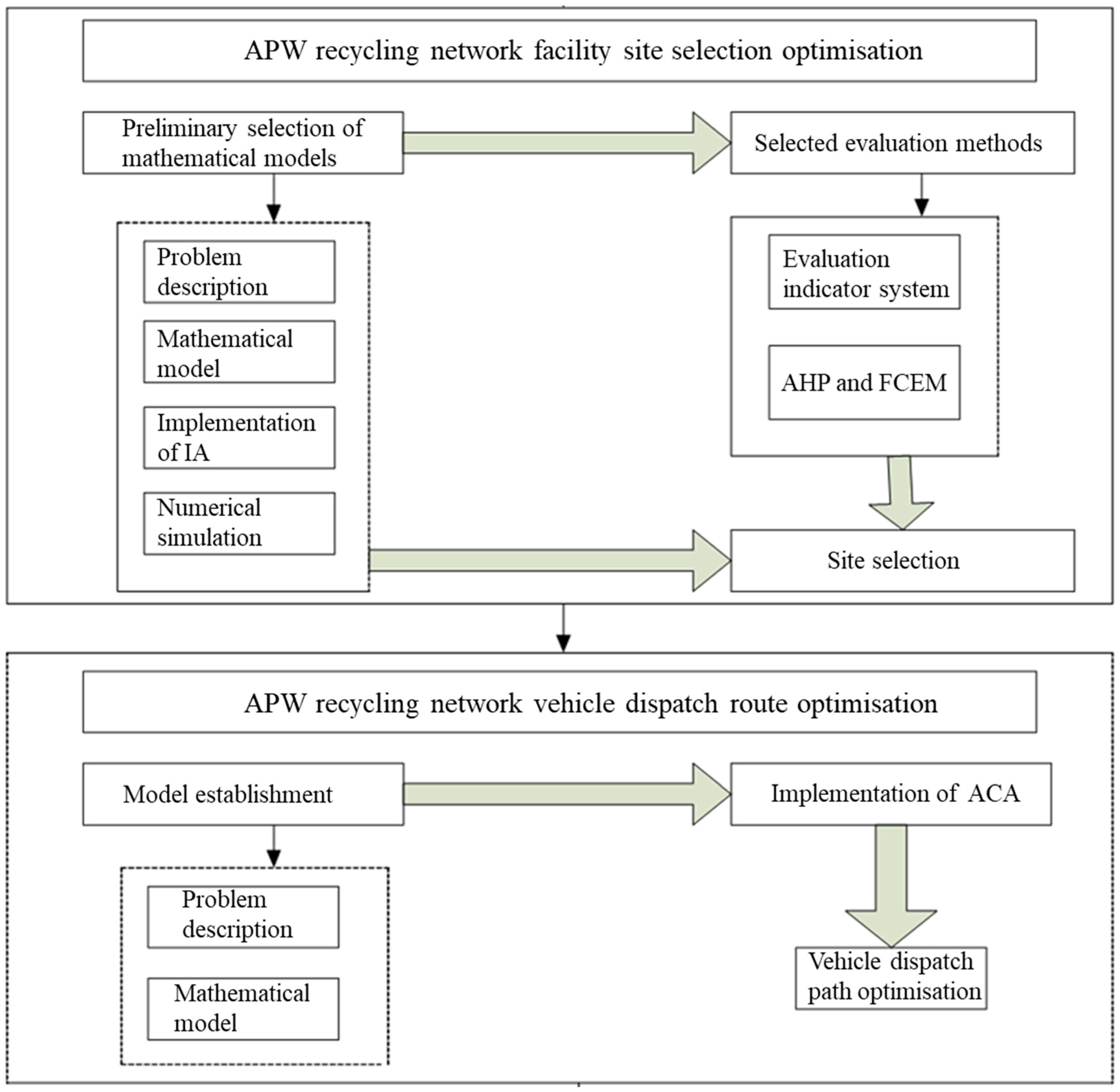
2.1. Model Formulation

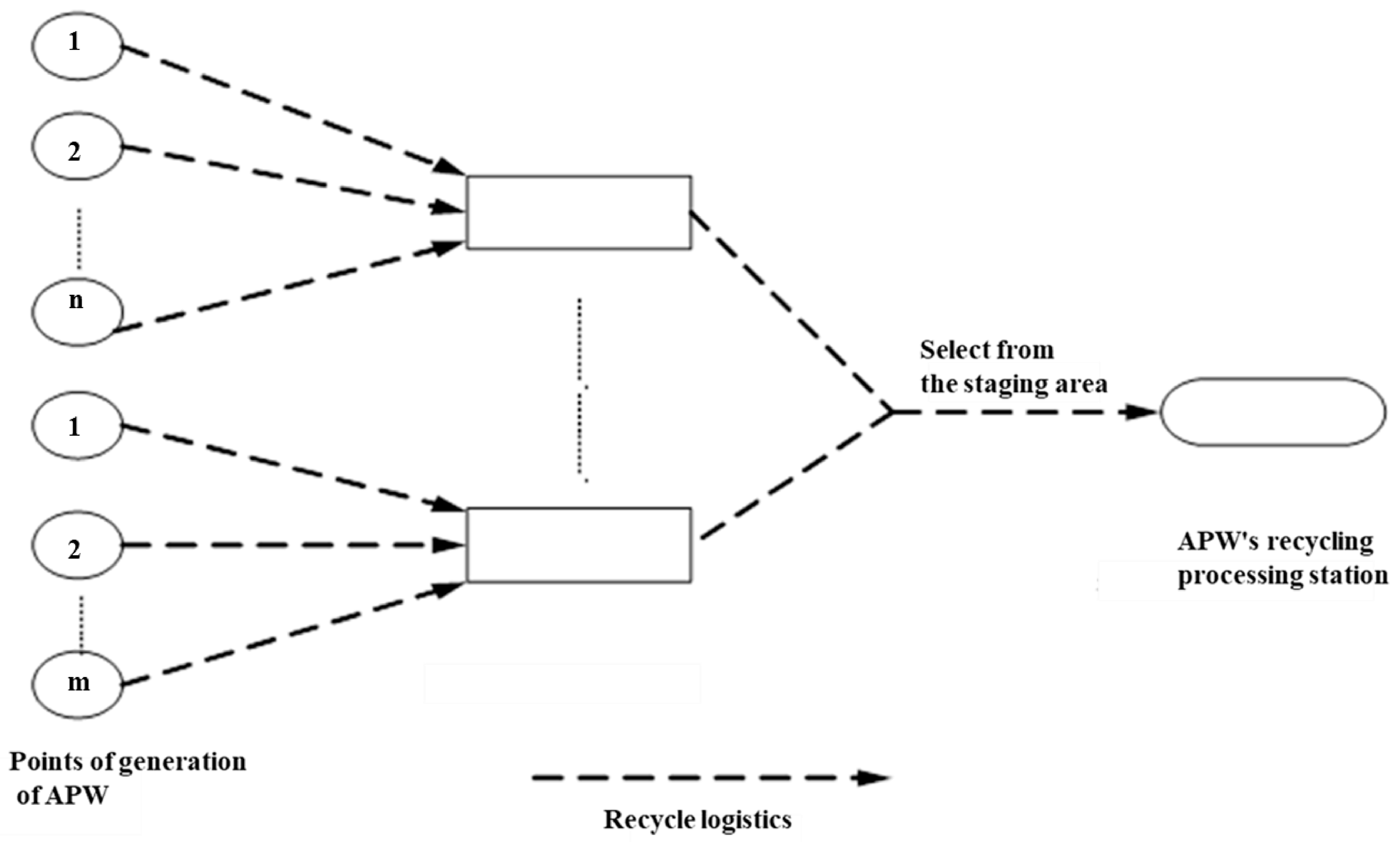
2.1.1. Construction of a Recycling Network for APW

Recycling APW generally consists of three stages, as shown in Figure 2. First, the APW generated by farmers is recycled. This usually means that specialized vehicles used for APW recycling go along certain routes to collect APW and transport it to APW staging areas, that is, transport and storage. Second is transhipment. APW is transported over long distances; that is, APW is transported from a temporary storage location to a distant APW treatment station using specialized vehicles for recycling. Finally, APWs were classified, and different treatment methods were applied to different types of APWs.

2.1.2. Primary Model Building and Immunization Algorithm

Description of the Problem

Because the amount of generated APW may be large, one recycling staging area does not necessarily have the capacity to recycle APW generated at all generation points; therefore, multiple recycling staging areas are required. In addition, APW is characterized by dispersed generation, small generation at each generation point, large overall generation, and a large number of types, which makes it very difficult to collect accurate data on APW generation. Therefore, in this study, numerical simulations are used to study the different types of APW generated for its recycling, assuming that there is no need to carry out special treatment of APW in the recycling process and that it is centrally recycled to the staging area and then classified.

Distance Calculations in Site Selection Models

(1)

Distance between two points on a plane

Straight-line distances are chosen when selecting sites within a large area, whereas folded distances are more suitable for sites within a small area. To make the calculated results closer to the actual distance, the Euclidean distance is generally multiplied by an appropriate coefficient (usually called the detour coefficient), which is used to indicate the traffic conditions. Its value is related to the traffic conditions. Thus, when the traffic conditions are unfavorable, it takes on a larger value and vice versa—it takes on a smaller value. In this study, the APW generation point was located in a rural area; therefore, the detour coefficient was 1.5 [54], and the formula for the distance between the two points was as follows:

$$d_{ij}=w_{ij}\sqrt{{(x_i-x_j)}^2+{(y_i-y_j)}^2}$$

(1)

where $w_{ij}$ is the detour coefficient for each pair of points $(x_i,y_i)$ and $(x_j,y_j)$.

(2)

Distance between any two points on Earth

Since the APW generation points are distributed over geographic space, their locations are represented by latitude and longitude coordinates. To accurately calculate the shortest spherical distance between any two points, the standard Haversine formula [55,56] is used in this study. The formula outperforms other approximation methods in terms of computational accuracy and numerical stability, and it is particularly suitable for geographic distance calculations. Let the coordinates of point P₁ be (φ₁, λ₁), where φ₁ is latitude and λ₁ is longitude. The coordinates of point P₂ are (φ₂, λ₂), where φ₂ is latitude and λ₂ is longitude. North latitude takes a positive value, south latitude takes a negative value, east longitude takes a positive value, and west longitude takes a negative value. All angle units need to be converted to the radian system. The calculation steps and formulas are as follows:

Calculate the latitude difference and longitude difference:

$$\begin{array}{ccccc}\Delta \phi & =& {\phi }_2& -& {\phi }_1\\ \Delta \lambda & =& {\lambda }_2& -& {\lambda }_1\end{array}$$

(2)

Compute the intermediate variable $a$:

$$a={\sin }^2\left({\displaystyle \frac{\Delta \varphi }{2}}\right)+\cos {\varphi }_1\cdot \cos {\varphi }_2\cdot {\sin }^2\left({\displaystyle \frac{\Delta \lambda }{2}}\right)$$

(3)

Compute the intermediate variable $c$:

$$c=2\cdot \arctan 2\left(\begin{array}{c}\sqrt{a},\sqrt{1-a}\end{array}\right)$$

(4)

Finally, the spherical distance $d$ between two points can be expressed as follows:

$$d=R\cdot c$$

(5)

Discrete Point Ensemble Coverage Model

The main idea of the ensemble coverage model is to select the minimum number of service points to cover all the served points for some points that are known to be in need of service so that the needs of all the served points can be satisfied [57].

The first is to determine the model parameters: $I$ represents the set of APW generation points, $I=\left\{i/1,\dots ,m\right\}$, where $m$ is the number of generation points; $J$ represents the set of APW facility points (temporary storage), $J=\left\{j/1,\dots ,n\right\}$, where $n$ is the number of candidate facility points; $q_i$ represents the amount of APW generated by generation point $i$; $d_{ij}$ represents the distance between generation point $i$ and facility point $j$. Because APW is generally generated in rural areas, a straight-line distance multiplied by a detour coefficient is used here, where the detour coefficient $w_{ij}=1.5$; $Q_j$ represents the maximum recycling capacity of staging area $j$; $r$ represents the service radius of the temporary storage.

The second step involves dealing with the decision variables. The decision variable $x_j$ is a 0–1 variable that indicates whether to build an APW recycling staging area at the APW generation site $j$. If an APW recycling staging area is built at the APW generation site $j$, then $x_j=1$; otherwise, $x_j=0$. Here, variable $y_{ij}$ is a 0–1 variable that indicates whether the APW generated at the APW’s generation site $i$ is transported to the APW’s recycling staging site $j$. If the APW generated at the APW’s generation site $i$ is provided with recycling services by the APW’s recycling staging site $j$, then $y_{ij}=1$; if the APW generated at the APW’s generation site $i$ is not provided with recycling services by the APW’s recycling staging site $j$, then $y_{ij}=0$.

Based on the assumptions of the above model, the meanings of the decision variables and parameters of the model, and with the optimization objective of minimizing the number of recycling staging areas of APW, the following model of recycling staging areas of APW is constructed to reduce the construction cost of recycling staging areas of APW.

Objective function:

$$Min{\displaystyle \sum _{j\in J}{x}_j}$$

(6)

Constraints:

$$x_j\ge y_{ij} \forall i\in I,\forall j\in J$$

(7)

$$y_{ij}\le x_j \forall i\in I,\forall j\in J$$

(8)

$${\displaystyle \sum _{i\in J}{y}_{ij}}\ge 1 \forall i\in I$$

(9)

$${\displaystyle \sum _{i=1}^m{q}_i{y}_{ij}+q_j\le Q_j{x}_j},\forall j\in J$$

(10)

$$x_{ij}\le [d_{ij}\le r] \forall i\in I,j\in J$$

(11)

where the objective function Equation (6) represents the minimum number of APW recycling staging areas; Equation (7) indicates that if generation point $i$ is served by storage point $j$, then $j$ must be established; Equation (8) ensures that unestablished storage points do not provide services; Equation (9) ensures that all generation points are covered; Equation (10) limits the total amount of recycling at each storage point $j$ to no more than its capacity $Q_j$. Equation (11) indicates that point $i$ generated by APW is only allowed to be served by temporary storage area $j$ when the distance $d_{ij}$ between point $i$ and temporary storage area $j$ does not exceed the service radius $r$.

2.1.3. Establishment of Evaluation Indicators for Treatment Station Siting

The methods used to solve the problem of siting APW recycling depots were hierarchical analysis and fuzzy comprehensive evaluation. The hierarchical analysis and fuzzy comprehensive evaluation methods were used in combination to evaluate the APW site selection options. First, the hierarchical analysis method was used to determine the sub-objectives and weights of the indicators of the APW recycling and staging plant, and then the fuzzy comprehensive evaluation method was used to conduct a comprehensive evaluation of the options for the location of the APW facility to make the final option more reliable and effective.

2.1.4. Vehicle Dispatch Path Optimization Model

The optimal design of the recycling network of APW also entails studying the vehicle scheduling path formulation problem, which is also a key problem in the decision-making of the recycling network of APW. The cost of vehicle transport accounts for a high proportion of the cost in the recycling process of APW, and the collection and transport of APW is an important link in the realization of the recycling economy, which not only can effectively alleviate the problem of the shortage of resources in our country but also improve the efficiency of the recycling process. In this section, an optimization model of the dispatch path of recycling vehicles for APW is developed, solved using the ACA, and validated based on the results of the siting of the recycling staging office facilities in the previous section.

Basic Assumptions of the Model

First, there are enough specialized vehicles for APW recycling at the APW processing station. Second, the location of the APW staging area and the stock of APW are known. Finally, there is only one APW processing station, from which the specialized vehicles for APW recycling depart and return to the APW processing station after completing the collection of APW.

Description of Parameters

(1)

Relevant parameters

$q_i$ represents the amount of APW in the APW recycling staging area, $Q_k$ represents the maximum load capacity of the APW recycling transport vehicle, $d_{ij}$ represents the distance between the APW recycling staging areas, and $c$ represents the unit transport cost per unit distance of the APW recycling transport vehicle.

(2)

Decision-making variables

$$y_{ik}=\left\{\begin{array}{l}1,if generation point i is collected by car k\\ 0,\hspace{1em}otherwise\end{array}\right.$$

(12)

Here, $y_{ik}$ is a 0–1 variable that indicates whether the APW at the APW generating site $k$ is collected by trucks. If the APW at the APW generator $i$ is collected by vehicle $k$, then $y_{ik}=1$. If the APW at the APW generator $i$ is not collected by vehicle $k$, then $y_{ik}=0$.

$$x_{ijk}=\left\{\begin{array}{l}1,if Vehicle k is from i to j\\ 0,\hspace{1em}otherwise\end{array}\right.$$

(13)

Here, $x_{ijk}$ is a 0–1 variable that indicates whether the APW collected by vehicle $k$ is travelling from the generating site $i$ to the generating site $j$. The APW collected by vehicle $k$ is the APW collected by vehicle $k$ from the generating site $i$ to generate site $j$. If yes, then $x_{ijk}=1$; if no, then $x_{ijk}=0$.

(3)

Vehicle transport cost

Vehicle delivery costs include variable and fixed costs, and fixed costs are mainly vehicle acquisition and information system costs. Assuming that the costs of vehicles of the same load type are the same and that APW’s recycling staging area requires $m$ vehicles to collect APW, the fixed cost is ${\displaystyle \sum _{k=1}^m{f}_k}$. The variation of vehicles in the transport costs is related to the distance; that is, the further the distance, the higher the variable cost. Assuming that the unit travelling cost per unit distance is $c$, and $d_{ij}$ is the distance between the two collection points, the variable cost can be expressed as $c\ast d_{ij}$.

Model Construction

Based on the assumptions of the above model, the meanings of the decision variables, and the representation of the parameters of the model, the following optimization model of the dispatch path of recycling vehicles for APW is constructed with the optimization objective of minimizing the total cost of vehicle transport for recycling APW, to minimize the total cost of vehicle transport for recycling APW.

The objective function:

$$\min Z={\displaystyle \sum _{k=1}^m{{\displaystyle f}}_k}+c{\displaystyle \sum _{k=1}^m{\displaystyle \sum _{i=1}^n{\displaystyle \sum _{j=1}^n{{\displaystyle x}}_{ijk}{{\displaystyle d}}_{ij}}}}$$

(14)

Constraints:

$${\displaystyle \sum _{i=0}^n{x}_{ijk}=y_{ik\le 1}}$$

(15)

$${\displaystyle \sum _{j=0}^n{x}_{ijk}}=y_{ik\le 1}$$

(16)

$${\displaystyle \sum _{k=0}^m{y}_{ik}=\left\{\begin{array}{l}0,if i is 1\dots n\\ m,if i is 0\end{array}\right.}$$

(17)

$${\displaystyle \sum _{i=1}^n\left(q_i{\displaystyle \sum _{j=1}^n{x}_{ijk}}\right)}\le Q_k$$

(18)

where the objective function in Equation (18) indicates that the sum of the fixed and variable costs of the APW recycling haulage vehicles is minimized; Equations (19) and (20) indicate that each APW recycling staging area is collected by only one APW recycling vehicle; Equation (21) indicates that each APW recycling staging area is allocated to and is allocated to only one APW recycling vehicle; and Equation (22) indicates that the amount of APW collected by each APW recycling car cannot be more than the maximum load capacity of the APW recycling vehicles.

2.2. Algorithmic Methods

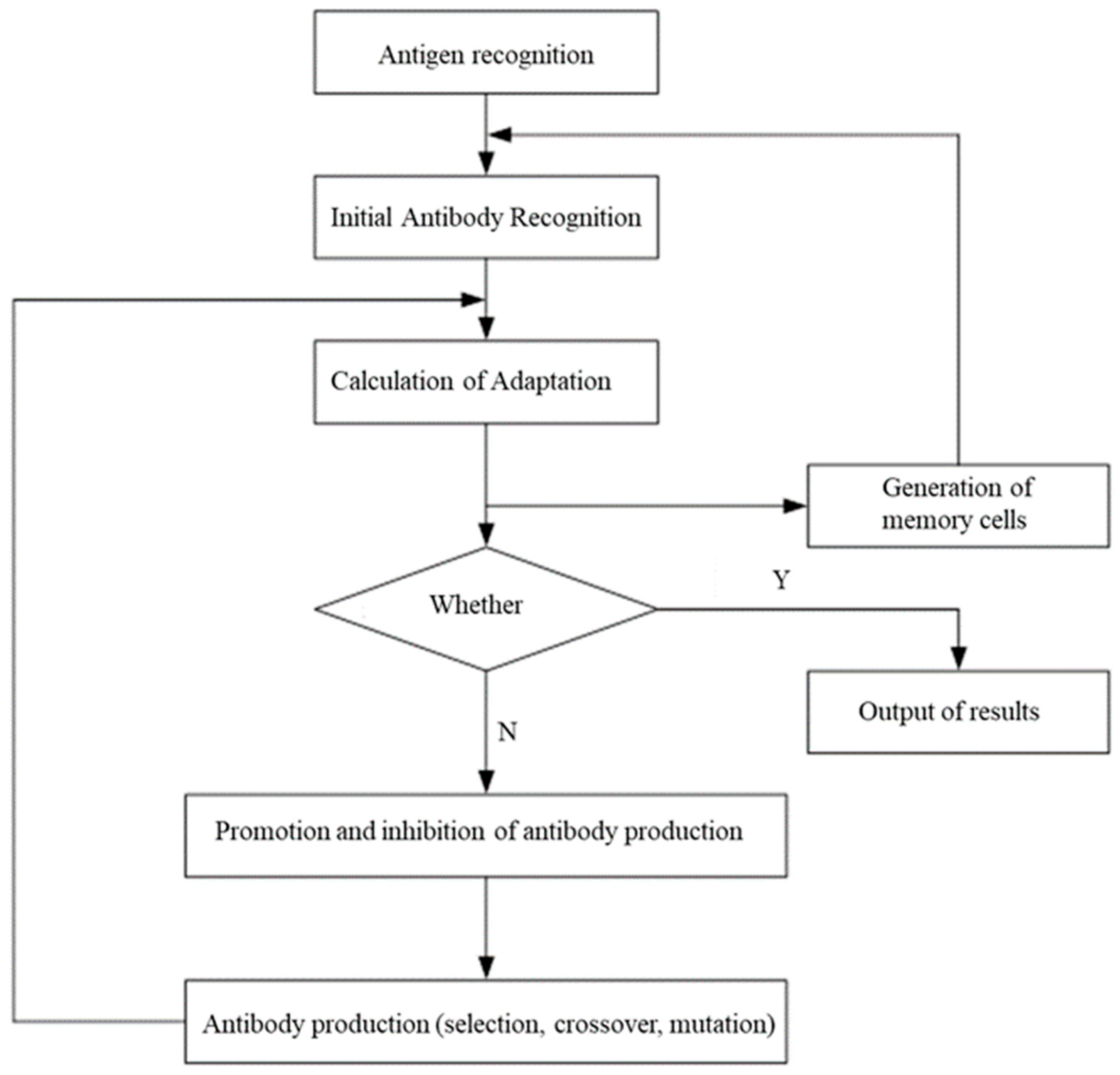
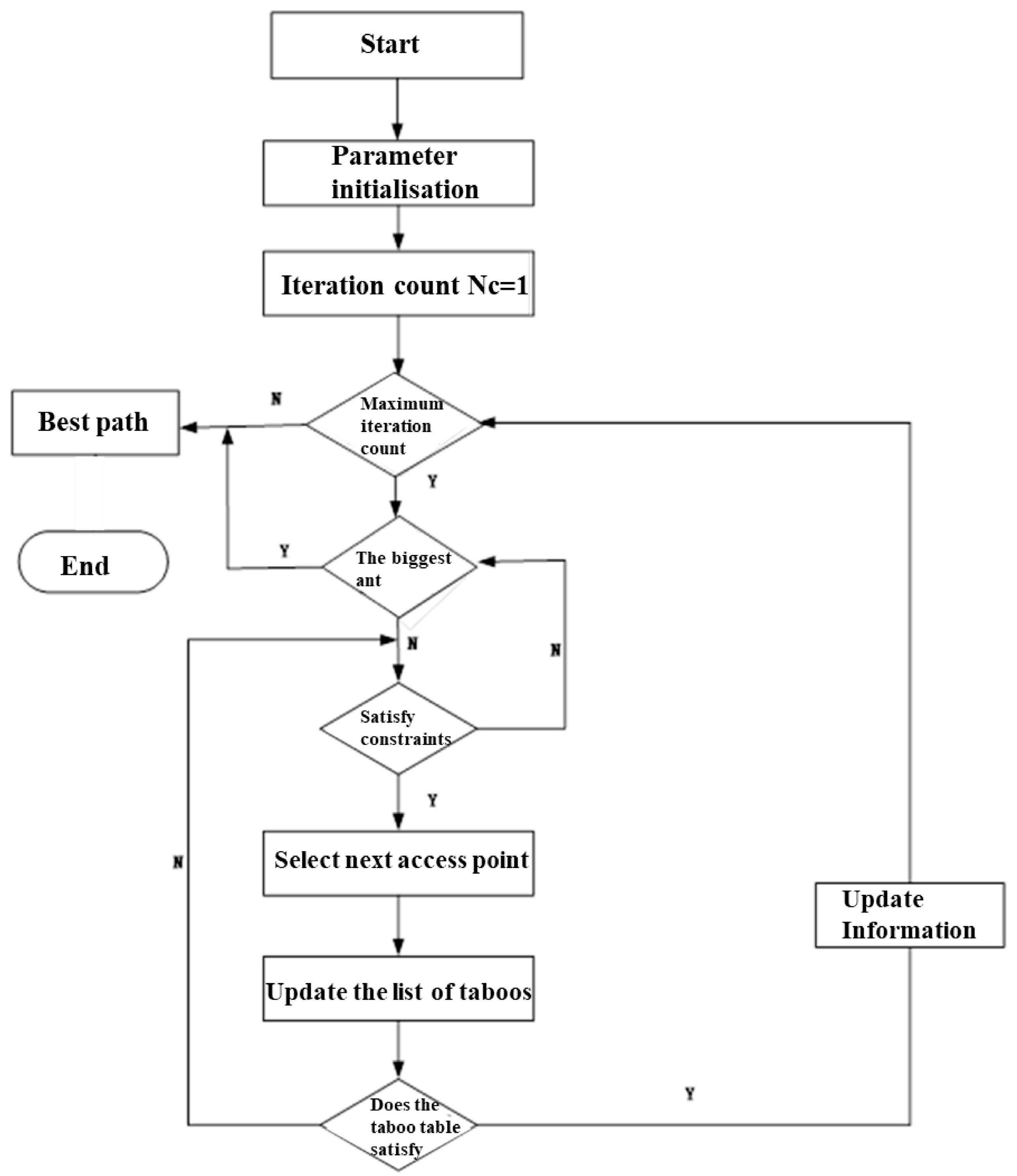
2.2.1. Immune Algorithm (IA)

The IA is inspired by human cell theory and network theory by mimicking the human immune system, and it ultimately seeks the global optimal solution by ensuring that the population is diverse [58,59]. A flowchart of the IA is shown in Figure 3. The specific implementation steps of IA are as follows [60,61]:

(1)

Problem analysis: analyze the relevant problem and the properties of its solution, and devise a suitable expression for the solution.

(2)

Initial antibody population generation: $m$ individuals are extracted from randomly generated $N$ individuals to form the initial population ($m$ is the number of individuals in the memory bank).

(3)

Antibody evaluation.

(4)

Parent population formation: the initial population generated earlier is arranged in the relevant descending order by a certain desired reproduction rate $p$, where the parent population is composed of $N$ individuals randomly generated earlier, and m individuals are deposited in the memory bank.

(5)

Termination condition check: determine whether the end condition is satisfied; if so, end; otherwise, proceed to the next step.

(6)

New population generation: perform relevant operations on the antibody population to obtain a new population, extract the individuals from the memory, and constitute a new generation of the population.

(7)

Return to evaluation step: once a new population is generated, it is transferred to Step (3).

The initial antibody population is generated in two scenarios: the first scenario is when the memory bank is non-empty, and the initial antibody population is selected from the memory bank to be generated; the second scenario is when the memory bank is empty, and the initial antibody population is randomly generated in the corresponding feasible solution space at this time. Each solution may form an antibody of length $p$, representing the sequence selected for the staging site.

The following is an evaluation of the diversity of solutions: The first is the affinity between the antibody and antigen. The degree of recognition of the antigen by the antibody is represented by the affinity between the antibody and the antigen, and the affinity function $A_v$ is designed in the siting model with the following formula [62]:

$$A_v={\displaystyle \frac{1}{F_v}}={\displaystyle \frac{1}{{\displaystyle \sum _{i\in N}{\displaystyle \sum _{j\in M_i}{w}_i{d}_{ij}{Z}_{ij}-c{\displaystyle \sum _{i\in N}\min \left\{\left({\displaystyle \sum _{j\in M_i}{Z}_{ij}}\right)-1,0\right\}}}}}}$$

(19)

where $F_v$ is the objective function. In the second term of the denominator, $c$ takes a relatively large positive number, giving some penalty for those cases in which the distance constraint solution is violated. $M$ is the penalty coefficient used to impose penalties on solutions that violate distance constraints. $Z_{ij}$ is an indicator variable with a range of 0–1. When the distance $d_{ij}$ between waste generation point $i$ and temporary storage point $j$ is greater than $r_j$, it takes the value 1; otherwise, it takes the value 0.

Affinity (which exists between antibodies) is mainly able to reflect the degree of similarity between antibodies, and the formula is [63]

$$S_{v,s}={\displaystyle \frac{k_{v,s}}{L}}$$

(20)

where $k_{v,s}$ is the number of bits in antibody $v$, which are identical to those in antibody $s$, and $L$ is the length of the antibody.

The proportion of similar antibodies in a population is the antibody concentration, which is denoted by $C_v$. The formula is [64]

$$C_v={\displaystyle \frac{1}{N}}{\displaystyle \sum _{j\in N}{S}_{v,s}}$$

(21)

where $N$ is the total number of antibodies.

$$S_{v,s}=\left\{\begin{array}{l}1,S_{v,s}>T\\ 0,otherwise\end{array}\right.$$

(22)

where $T$ is a pre-set threshold value.

Next, the expected reproductive rate for each individual was calculated. In a population, the two components $A_v$ and $C_v$ determine the expected reproduction rate of each individual using the following formula:

$$P=\partial {\displaystyle \frac{A_v}{{\displaystyle \sum A_v}}}+(1-\partial ){\displaystyle \frac{C_v}{{\displaystyle \sum C_v}}}$$

(23)

where $\partial$ is a constant.

Finally, immunological operations were performed. Immune operation mainly refers to three types of selection, crossover, and mutation [65]. Therefore, this study adopted the IA to select the staging area site, leveraging its advantages in maintaining population diversity through mechanisms like affinity calculation, antibody concentration evaluation, and expected reproduction rate selection. The essence of the site selection problem is to find the smallest set of facilities that covers all demand points, which is a typical combinatorial optimization problem. The core advantage of the IA lies in its antibody diversity maintenance mechanisms, such as concentration inhibition and expected reproduction rate calculation. This mechanism can effectively explore the solution space, can avoid premature convergence, and is particularly suitable for solving problems that require global search and have a discrete solution space. In contrast to other evolutionary algorithms such as genetic algorithms (GAs) [66] or simulated annealing (SA) [67], while GAs’ crossover and mutation operations are powerful, the IA’s immune-regulation mechanism offers a more natural solution for handling strong constraints such as coverage radius, capacity limits, and preventing premature population homogenization. Although SA is advantageous in escaping local optima, its single-point search characteristic can lead to lower computational efficiency and less stable solution quality when solving large-scale discrete site-selection problems compared to population-based methods like the IA.

2.2.2. Methodology for Analyzing the Siting of Treatment Stations

Hierarchical Analysis (HA)

HA is a common evaluation of the decision-making analysis method, which is a combination of qualitative analysis and quantitative analysis. The biggest advantage is that there can be many complex, ambiguous correlations in a quantitative analysis of the problem [68].

First, it is necessary to establish a hierarchy of progression. Next, a judgement matrix is constructed. Subsequently, single-sort weights and consistency tests are performed. Finally, total sort weights and consistency tests are performed. Assuming that the consistency index of certain elements selected in the judgement hierarchy for the single sorting of the target layer above is denoted by $C{I}_j$ (where $j$ is the index of criteria in the current hierarchy level), and the corresponding average random consistency index at this time is denoted as $R{I}_j$, it can be derived that the random consistency ratio of the total sorting of the final judgement hierarchy is

$$C{R}_j={\displaystyle \frac{{\displaystyle \sum _{j=1}^n{a}_{j}C{I}_j}}{{\displaystyle \sum _{j=1}^n{a}_{j}R{I}_j}}}$$

(24)

In the formula, $a_j$ is the weight of the $j$th layer indicator.

Fuzzy Integrated Evaluation Method (FIEM)

The main idea of the FIEM is to use the principles of fuzzy relationship synthesis reasonably and effectively on the basis of fuzzy mathematical concepts to quantify those factors that are not easy to quantify, have complex relationships, and have unclear boundaries [69]. It has some unique characteristics, such as judging the selected objects one by one and giving a unique evaluation value [70].

Assume that the object of judgement is $K$: factor set $R=\left\{r_1,r_2,\dots ,r_n\right\}$ and judgement rating set $U=\left\{u_1,u_2,\dots ,u_m\right\}$. Each factor in $R$ can only be fuzzy-judged according to the rating indicators in the judgement set, thus enabling a judgement matrix to be derived:

$$V=\left(\begin{array}{ccc}{v}_{11}& \dots & v_{1m}\\ ⋮& \ddots & ⋮\\ v_{n1}& \dots & v_{nm}\end{array}\right)$$

(25)

where $v_{ij}$ denotes the degree of affiliation between $r_i$ and $u_j$. $(R,U,V)$ constitutes a fuzzy comprehensive judgement model after determining the weights of the factors, denoted as $P=\left\{p_1,p_2,\dots ,p_n\right\}$, which satisfies ${\displaystyle \sum _{i=1}^n{p}_i=1}$, which yields $\overline{A}=P·V=(\overline{a_1},\overline{a_2},\dots ,\overline{a_m})$, which, after normalization, yields $A=(a_1,a_2,\dots ,a_m)$ and finally determines the judgement grade of the object $K$.

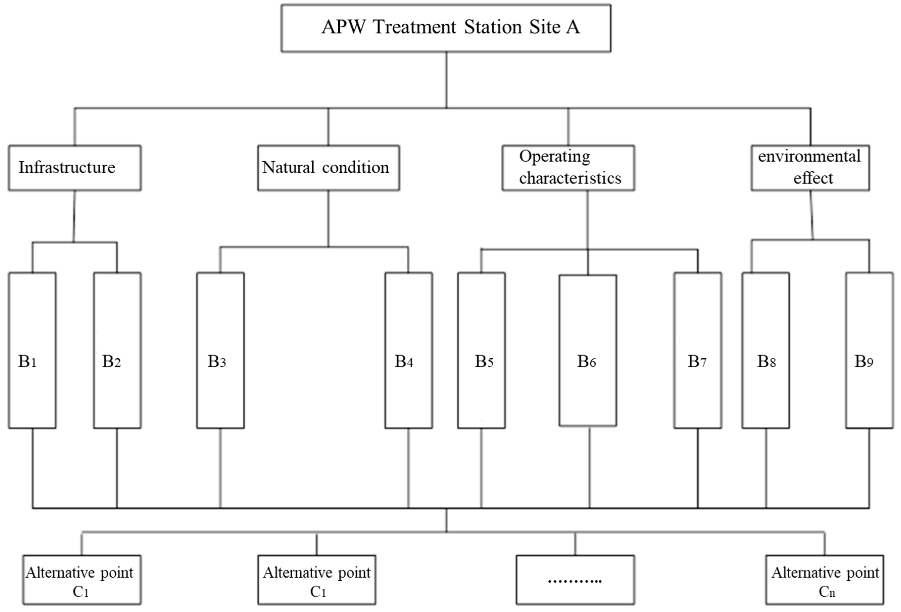
2.2.3. Evaluation System and Hierarchical Structure

Based on the influencing factors of the APW recycling network facility siting, its evaluation system was determined, and a hierarchy was established. On the target level is the site of APW’s processing station. At the judgement level, the four evaluation indicators of infrastructure, natural conditions, operating characteristics, economic, and environmental effects are selected, and the alternative point in the program level is APW’s recycling staging area, as shown in Figure 4.

Infrastructure includes B1 (transportation) and B2 (public infrastructure). The location of the APW recycling and processing station requires high transport conditions and should be chosen in a place with more developed transport. The more types of loads on transport vehicles, the higher the score. Meanwhile, the public infrastructure conditions of the recycling and treatment station of APW mainly refer to the cost of land for the construction of the APW recycling and treatment station. The lower the cost of land, the lower the cost of establishing the APW recycling and treatment station, and the higher the score value obtained.

Natural conditions include topographical and meteorological features, and APW recycling stations should be built on flat terrain with a suitable area. Ideally, the site should be completely flat, followed by a slightly sloping or undulating site. At the same time, meteorological characteristics are also a factor that needs to be focused on during the site selection process for recycling and treatment stations of APW; the meteorological condition factors that need to be taken into account mainly refer to the direction of the wind and the size of the wind; when the wind speed is smaller, the impact on the surrounding environment is smaller, the more favorable it is for the establishment of the recycling and treatment station for APW, and the greater the score value.

Operational characteristics include the characteristics of agricultural production waste (B5), level of recycling and treatment services (B6), and logistics costs (B7). As recycled APW has different characteristics, different types of APW recycling and treatment stations should be distributed in different geographical areas. APW needs to be transported to the treatment station on time for treatment after being collected by the recycling staging area. The closer the staging area is to the treatment station, the shorter the response time of the treatment station to provide service to the staging area, and the more efficient the service, so the higher the score value. The closer the address of the staging area and the treatment station is to the area served, the smaller the recycling logistics cost, and the higher the score value. The closer the location of the selected storage and processing stations to the area they serve, the smaller the recycling logistics costs and the higher the score.

Economic and environmental effects refer to the impact of the construction of APW recycling and processing stations on the local environment and residents’ lives. If the impact on the local environment and residents’ lives is very small, it means that it is possible to build a recycling and processing station for APW in this area, and a higher score will be obtained.

Based on the above analyses and the principles of the hierarchical analysis method described above, the following judgement matrix was established: Because the environmental impact, recycling service level, logistics cost, and other factors are more important than other factors in the process of building the APW recycling and treatment station, the scores will be relatively high in the process of judgment, as shown in

Table 1. Judgement matrix of factors influencing the construction of treatment stations.

A	B1	B2	B3	B4	B5	B6	B7	B8	B9
B1	1	3	5	9	2	7	1/4	1/7	3
B2	1/3	1	2	5	3	6	1/3	1/7	5
B3	1/5	1/2	1	1/2	3	5	1/5	1/9	2
B4	1/9	1/5	2	1	2	7	1/5	1/9	2
B5	1/2	1/3	1/3	1/2	1	1/3	1/5	1/9	3
B6	1/7	1/6	1/5	1/7	3	1	3	1/7	7
B7	4	3	5	5	5	3	1	1/5	5
B8	7	7	9	9	9	7	5	1	9
B9	1/3	1/5	1/2	1/2	1/3	1/7	1/5	1/9	1

.

2.2.4. Methods for Solving the Vehicle Scheduling Path Problem

Generic heuristic algorithms mainly include the ACA, IA, and hybrid algorithms, which combine the characteristics of several algorithms. Research has shown that the general heuristic algorithm can effectively deal with large-scale vehicle scheduling path problems in a relatively short time and can produce the optimal solution or near-optimal solution of this type of problem, so it has been greatly developed in both theory and practical applications [71]. The Vehicle Routing Problem (VRP variant) inherently possesses a network path structure and positive feedback demand. The core concept of the ACA—ants use pheromone accumulation to find the shortest path—aligns closely with the optimization objective of the VRP (minimizing total distance/cost). Its distributed, self-organizing positive feedback mechanism enables efficient exploration of large-scale path combination spaces and gradual reinforcement of optimal paths. While GAs can also solve the VRP, their chromosome representation of paths (e.g., sequential encoding) and genetic operations (crossover, mutation) often require complex repair mechanisms to maintain path feasibility (e.g., avoiding subloops, satisfying capacity constraints), thereby increasing algorithmic complexity and computational burden. SA also faces the challenge of designing efficient neighborhood structures and cooling strategies to balance exploration and exploitation in VRP solutions. The following mainly introduces the ACA used in this study [72,73,74], which is a heuristic algorithm.

The solution flowchart of ACA is shown in Figure 5.

Let $m$ be the overall number of ants and $n$ represent the number of visited points. $d_{ij}=\left(i,j=1,2,\dots ,n\right)$ is the distance between the visited points $i$ and $j$, the pheromone concentration contained in this path of the visited points $i$ and $j$ at the moment t is denoted by ${\tau }_{ij}(t)$, and ${\tau }_{ij}(0)={\tau }_0$ is the pheromone concentration that each visited point has in its path at the initial moment.

Ant $k=\left(k=1,2,\dots ,m\right)$, and the next place that will be visited can only be decided based on the concentration of pheromone contained at each visit point, $P_{ij}^k(t)$ denotes the probability of ant $k$ moving from visit point $i$ to $j$ at the moment of $t$, which is calculated as

$$P_{ij}^k(t)=\left\{\begin{array}{l}{\displaystyle \frac{{\left[{\tau }_{ij}(t)\right]}^{\alpha }\times {\left[{\eta }_{ij}(t)\right]}^{\beta }}{{\displaystyle \sum _{s\in allo{w}_k}{\left[{\tau }_{is}(t)\right]}^{\alpha }\times {\left[{\eta }_{is}(t)\right]}^{\beta }}}},s\in allo{w}_k\\ 0,otherwise\end{array}\right.$$

(26)

In Equation (23), the heuristic function is denoted as ${\eta }_{ij}(t)$, the expected degree of the ants from visiting the points is denoted as ${\eta }_{ij}(t)={\displaystyle \frac{1}{d_{ij}}}$, and the set of points to be visited by ant $k$ is denoted as $allo{w}_k(k=1,2,\dots ,m)$.

The degree of pheromone volatilization on the access path is indicated by the parameter $\rho (0<\rho <1)$. Since the concentration of pheromone on the path evaporates over time, the pheromone needs to be updated with the following equation:

$$\left\{\begin{array}{l}△{\tau }_{ij}={\displaystyle \sum _{k=1}^n△{\tau }_{ij}^k}\\ {\tau }_{ij}(t+1)=(1-\rho ){\tau }_{ij}(t)+△{\tau }_{ij}\end{array}\right.$$

(27)

where $△{\tau }_{ij}^k$ denotes the pheromone concentration of the $k$th ant on the paths of access points $i$ and $j$, and $△{\tau }_{ij}$ denotes the sum of all pheromone concentrations.

For the ant pheromone problem, three models are proposed using the following formulas:

(1)

In the first model, the $△{\tau }_{ij}^k$ formula is

$$△{\tau }_{ij}^k=\left\{\begin{array}{l}{\displaystyle \frac{Q}{L_k}},the kth ant visits the jth ant from i\\ 0,otherwise\end{array}\right.$$

(28)

where $Q$ is a constant and denotes the total amount of pheromone released when an ant cycles once; $L_k$ is the length of the path through which the $k$th ant passes.

(2)

In the second model, $△{\tau }_{ij}^k$ is calculated as

$$△{\tau }_{ij}^k=\left\{\begin{array}{l}{\displaystyle \frac{Q}{d_{ij}}},the kth ant visits the jth ant from i\\ 0,otherwise\end{array}\right.$$

(29)

(3)

In the third model, $△{\tau }_{ij}^k$ is calculated as

$$△{\tau }_{ij}^k=\left\{\begin{array}{l}Q,the kth ant visits the jth ant from i\\ 0,otherwise\end{array}\right.$$

(30)

3. Example Description and Solution

3.1. Experimental Setup

3.1.1. Data and Parameters for Site Selection

APW is generated at multiple points and is widely distributed; however, the amount of APW produced at each individual point is relatively small. The uncertainty surrounding APW recovery stems from the fact that farmers engaged in planting and breeding may have low levels of education and low environmental awareness, resulting in a lack of awareness regarding APW recovery. This leads to unclear total APW resources, as well as uncertainty regarding the actual amount of APW produced each year, how these wastes are distributed, how they are disposed and treated, and the ultimate impact on the environment. However, these aspects lack accurate records and data. Even if data exist, discrepancies arise due to differing calculation standards, further complicating APW recovery efforts.

Based on this, we selected 110 APW generation points, denoted by $I$, where $I=\left\{i/1,\dots ,m\right\}$, $m$ has a value of 110, and $q_i$ represents the amount of APW in the $i$th region. The range of values for APW is divided into two cases: 150–195 kg and 200–260 kg; $Q_j$ represents the maximum recycling capacity limit of the APW recycling and temporary storage facility, where $Q_j=3000$ kg; and $r$ represents the service radius of the APW recycling and temporary storage facility, where $r=9$ km. Numerical simulation methods were used to conduct preliminary site selection for temporary storage facilities in an agricultural waste recycling network. The relevant data are provided in Appendix A and Appendix B.

The parameters used in this study follow the consensus in the field of agricultural waste recycling. The detour coefficient of 1.5 is consistent with the topological characteristics of rural roads [75]; the variation rate of the IA of 0.01 balances population diversity and convergence stability [76]; and the coverage radius of 9 km does not exceed the economic threshold for land transportation [77].

The IA was used to solve the site selection model for the APW recovery and temporary storage. The specific solution steps were as follows.

Step 1: antibody representation. Each APW recovery and temporary storage site selection scheme was encoded into an antibody of length m, where m represents the number of APW generation points. The sequence of candidate sites for APW recovery and temporary storage was composed of antibodies. An initialization operation was performed on the antibody group to generate n antibodies randomly.

Step 2: the affinity was calculated. The sequence numbers of APW generation points in one antibody were compared with those in another antibody individually. Antibody affinity was calculated by dividing the sum of the number of APW points with identical sequence numbers by the length of the antibody.

Step 3: calculation of antibody concentration. Using the formula for calculating antibody concentration introduced in the IA, that is, $C_v={\displaystyle \frac{1}{N}}{\displaystyle \sum _{j\in N}{S}_{v,s}}$ (where $N$ is the total number of antibodies) and $S_{v,s}=\left\{\begin{array}{l}1,S_{v,s}>T\\ 0,otherwise\end{array}\right.$ (where $T$ is a preset threshold), the antibody concentration was calculated.

Step 4: generation of memory cells. In Step 3, if the concentration of one type of antibody exceeded $T$, it indicated that the antibody had a significant survival advantage within the population, and a relatively optimal solution had been achieved. At this point, a memory cell was generated to record the local optimal solution. Additionally, memory cells can also function as inhibitory cells, suppressing antibodies with high affinity for the memory cell and reducing their survival probability, thereby ensuring that the IA does not become trapped in a local optimal solution.

Step 5: selection, crossover, and mutation. Antibodies generated earlier were selected using the expected reproduction rate selection method. For antibodies that survived the selection, a sequential crossover method was used to randomly pair and crossover them. The final mutation operation was performed using the swap-mutation method.

Step 6: evaluate relevant conditions. When the number of evolutionary generations reached a predefined maximum value, the final results were outputted. If the maximum value was not reached, the process continued to Step 2.

The numerical values of the parameters we used are as follows: population size (size pop) = 60, memory capacity over best = 10, maximum iteration count (MAXGEN) = 100, crossover probability (pcross) = 0.7, mutation probability (pmutation) = 0.01, diversity evaluation parameter (ps) = 0.95, maximum recovery capacity of the temporary storage area (Q) = 3000 kg, and coverage radius (r) = 9 km. The simulation was implemented using MATLAB R2022a.

3.1.2. Data and Parameters for Vehicle Routing

Because the areas where APW is generated are primarily rural, the detour coefficient $w_{ij}=1.5$ is used. The cost per vehicle at the APW processing station includes a vehicle purchase cost of CNY 2500/month, an average insurance cost of CNY 5500/year, a labor cost of CNY 3500/month, and a vehicle operating cost per unit distance of $c$, where $c$ is set at CNY 2.5/km. $Q_k$ represents the load capacity of a fully loaded vehicle, and $Q_k$ is set to 12, 13, and 10 t, respectively. This study assumes that there is only one APW treatment station, and the departure and arrival points of the APW-dedicated vehicles are both APW recycling treatment stations, that is, the dedicated collection vehicles return to the APW recycling treatment station after collecting the APW. Vehicle scheduling path optimization is performed based on the 19 temporary storage locations and quantities determined in the previous section (as shown in

Table 2. Alternative locations for APW recovery and storage sites.

APW Recycling Drop-Off Locations	APW Recycling Drop-Off Location Coordinates (${\mathit{X}}_{\mathit{i}}, {\mathit{Y}}_{\mathit{j}}$)
30	(80.5606, 3.7411)
6	(16.6211, 7.8272)
17	(36.0750, 7.0585)
25	(59.4368, 7.8994)
3	(73.4919, 6.9218)
2	(89.1218, 9.8461)
28	(16.3800, 8.1635)
13	(63.3359, 3.4798)
29	(75.3796, 9.7899)
27	(91.4370, 8.3471)
11	(18.5414, 7.7495)
26	(20.0632, 3.6639)
23	(56.7005, 7.2601)
24	(77.6402, 8.2543)
14	(15.5781, 6.8121)
21	(34.9283, 9.5245)
8	(99.0339, 4.1811)
16	(73.7465, 5.7014)
9	(64.4371, 8.9227)

).

The specific solution steps are as follows:

Step 1: Initialize the parameters in the algorithm, including the number of vehicles, pheromone evaporation factor, pheromone importance factor on the access path, total amount of pheromone released, importance of the heuristic factor, and maximum number of iterations for the algorithm.

Step 2: The starting point is the APW processing station, where all APW recycling storage areas must be visited. If the number of selected vehicles is too small, the number of vehicles can be appropriately adjusted. Establish a set of APW recycling storage areas that need to be served and simultaneously establish a tabu list for vehicle $k$, recording the nodes that vehicle $k$ has currently passed through.

Step 3: Based on the load capacity restrictions of the APW collection vehicles, determine the set of APW collection and storage sites that the vehicle can visit next. If the set is not empty, proceed to the next step; if the set is empty, proceed to step 5.

Step 4: According to the transition probability and rules in the ACA, determine the APW recycling temporary storage location that the vehicle will visit next, add the visited APW recycling temporary storage location to the current set, update the vehicle’s tabu list, and move the vehicle to the visited APW recycling temporary storage location.

Step 5: Check whether the set of APW recycling storage locations that must be served is empty. If it is empty, all APW recycling storage locations are served and the process returns to the starting point. Additionally, if the vehicle $k$ is less than or equal to $n$, the process returns to Step 2 to restart; otherwise, it proceeds to the next step. If the set of APW recycling storage locations that must be served is not empty, the process returns to Step 3.

Step 6: Record the iterative optimal solution for each vehicle, and continuously update the pheromone content along the path.

Step 7: The optimal function objective values are compared. If this value is better than the previous one, both the optimal objective function value and optimal path are updated until the specified maximum number of iterations is reached. Otherwise, clear the previously established tabu list and proceed to Step 3.

In this study, the number of ants was set to 95, the pheromone evaporation factor $rho=0.1$, the total pheromone release $Q$ was 50, the pheromone importance factor $ahpha$ was 5, the heuristic factor importance $beta$ was 7, the maximum number of iterations was 200, and the load capacity of the vehicle was 12 t.

3.2. Results and Analysis

3.2.1. Site Selection Results

The simulation results are shown in Figure 6 and Figure 7. From the experimental results, it can be seen that the algorithm reaches the convergence effect when iterating approximately 55 times; that is, the optimal fitness value and the average fitness value do not change significantly. When the amount of APW generated was in the range of 150–195 kg, 16 locations were selected as the recycling staging places of APW, and the results are shown in Figure 8 after being solved using MATLAB R2022a software.

The location coordinates of APW recycling temporary storage site 19 are (81.3072, 9.2860), that is, 19 (81.3072, 9.2860). Similarly, the location and coordinates of other APW recycling staging sites are 23 (56.7005, 7.2601), 26 (20.0632, 3.6639), 9 (64.4371, 8.9227), 30 (80.5605, 3.7411), 2 (89.1218, 9.8461), 12 (11.0286. 4.6616), 8 (99.0339, 4.1811), 16 (73.7465, 5.7014), 29 (75.3796, 9.7899), 28 (16.3800, 8.1635), 3 (73.4919, 6.9218), 25 (59.4368, 7.8994), 6 (16.6211. 7.8272), 21 (34.9283, 9.5245), and 11 (18.5414, 7.7495).

Based on the results of the solution, the locations of the APW recycling and storage sites were selected to be 19, 23, 26, 9, 30, 2, 12, 8, 16, 29, 28, 3, 25, 6, 21, and 11, as shown in Figure 8 (where the boxes represent the APW recycling and storage sites, and the circles represent the points where the APW is generated).

The recycling staging area for each APW covers the points generated by the APW, as listed in

Table 3. APW’s 16 recycling staging areas covering APW generation points.

Temporary Storage Area	APW Generation Point
19		19	42	46	71	73	83	96
23		18	23	55	70	85	92	93	100
26		26	40	48	50	67	108
9		9	13	37	47	56	77	97	99
30		30	41	60
2		1	2	20	22	27	38	54	82	98	102	106
12		12	58	68
8		5	8	15	33	51	63	65	72	76	78	80	103	105
16		16	31	32	34	74
29		24	29	35	39
28		28	75	88	91
3		3	57	61	69	110
25		25	53	81	89
6		6	14	49	66
21	7	10	17	21	43	44	45	52	64	79	94	101	104	107	109
11		4	11	36	59	62	84	86	87	90	95

.

When the amount of APW generated is 200–260 kg, 19 locations need to be selected as the APW recycling staging area, which was solved using MATLAB R2022a software.

In this case, the location and coordinates of APW recycling staging site 30 are (80.5606, 3.7411), that is, 30 (80.5606, 3.7411). Similarly, the location and coordinates of the recovery staging area of the other APWs are 6 (16.6211, 7.8272), 17 (36.0750, 7.0585), 25 (59.4368, 7.8994), 3 (73.4919, 6.9218), 2 (89.1218, 9.8461), 28 (16.3800, 9.1635), 13 (16.5606, 3.7411), or 30 (80.5606, 3.7411). 28 (16.3800, 8.1635), 13 (63.3359, 3.4798), 29 (75.3796, 9.7899), 27 (91.4370, 8.3471), 11 (18.5414, 7.7495), 26 (20.0632, 3.6639), 23 (56.7005, 7.2601), 24 (77.6402, 8.2543), 14 (15.5781, 6.8121), 21 (34.9283, 9.5245), 8 (99.0339, 4.1811), 16 (73.7465, 5.7014), and 9 (64.4371, 8.9227). Based on the results of the solution, the locations of the APW recovery staging areas were selected as 30, 6, 17, 25, 3, 2, 28, 13, 29, 27, 11, 26, 23, 24, 14, 21, 8, 16, and 9, and the specific locations are shown in Figure 9 below (where the squares represent the APW recovery staging areas, and the ellipses represent the APW generating points):

The points at which each APW recycling staging area covers the generation of APW are shown in

Table 4. Nineteen APW recovery staging areas covering APW generation points.

Temporary Storage Area	APW Generation Point
30	30	41	46
6	6	49
17	17	43	44	45	64	85	92	101	107	109
25	25	53	81	89
3	3	57	61	69	110
2	2	20	54	82
28	28	88	91
13	13	47	56	97	99
29	29	35	39
27	1	22	27	38	63	78	98	102	106
11	4	11	36	59	62	84	86	87	90	95
26	26	40	48	50	67	108
23	18	23	55	70	93	100
24	19	24	31	42	60	71	73	83	96
14	12	14	58	66	68	75
21	7	10	21	52	79	94	104
8	5	8	15	33	51	65	72	76	80	103	105
16	16	32	34	74
9	9	37	77

.

In summary, the results of the temporary storage site selection (Figure 8 and Figure 9) strictly satisfy the set coverage model constraints (service radius r = 9 km), and all agricultural waste generation points are effectively covered (Table 2 and Table 3). The spatial distribution shows significant balance: for example, x ∈ [15, 30], y ∈ [7, 9] corresponds to high-yield agricultural waste production areas (points with yields ≥ 240 kg account for 68% of the total), and a dense network of collection points is adopted to reduce short-distance transportation costs; (e.g., in the western region where x > 90) due to low yields (≤210 kg), a single-point wide-coverage strategy is adopted (e.g., Site 8 covers 15 generation points) to reduce facility construction costs.

The 19 APW staging sites were analyzed as an example, and after comparative analysis of the four evaluation indicators (infrastructure, natural conditions, operational characteristics, and economic/environmental effects) outlined in Section 2.2.3, it was decided to select three APW staging sites, 8 (99.0339, 4.1811), 28 (16.3800, 8.1635), and 11 (18.5414, 7.7495), from the 19 APW staging sites selected earlier, as the alternative addresses where the APW processing stations were built, denoted as C1, C2, and C3, respectively. After various consultations, the indicators of infrastructure, natural conditions, operational characteristics, and economic and environmental effects were selected in the judgement layer, according to the indicator system for the site selection of recycling and treatment stations for APW established earlier. By comparing the three alternative addresses (C1, C2, and C3) in the scheme layer with the transport conditions (TCs), meteorological characteristics (MCs), environmental benefits (EBs), recycling and treatment service level (RTSL), and terrain features (TFs), the following evaluation matrix was established by combining the evaluation matrix of the factors influencing the construction of the treatment station and solved by using the hierarchical analysis method and the fuzzy comprehensive evaluation method. Let the factor set be $U=\left\{TC, MC, EB, RTSL, TF\right\}$ and the evaluation set be $V=\left\{very good, good, fair, poor\right\}$.

The corresponding weights of the factors were expressed as the following fuzzy sets after consultation with the relevant people: $A=\left(0.23,0.25,0.3,0.12,0.10\right)$.

For each factor, the following evaluation matrix was derived after evaluation:

$$\begin{array}{c}{R}_a=\left(\begin{array}{l}0.3,0.5,0.2,0\\ 0.2,0.3,0.4,0.1\\ 0.2,0.4,0.2,0.2\\ 0,0.2,0.5,0.3\\ 0,0.1,0.4,0.5\end{array}\right)\\ R_b=\left(\begin{array}{l}0,0.3,0.4,0.3\\ 0.4,0.5,0.1,0\\ 0.5,0.4,0.1,0\\ 0,0.1,0.3,0.6\\ 0.2,0.3,0.4,0.1\end{array}\right)\\ R_c=\left(\begin{array}{l}0.2,0.3,0.4,0.1\\ 0,0.2,0.4,0.4\\ 0.1,0.2,0.3,0.4\\ 0.4,0.5,0.1,0\\ 0.3,0.4,0.2,0.1\end{array}\right)\end{array}$$

The fuzzy set of fuzzy comprehensive evaluation results was obtained after performing comprehensive evaluation:

$$\begin{array}{c}{B}_a=A·R_a=\left(0.23,0.25,0.3,0.12,0.10\right)\left(\begin{array}{l}0.3,0.5,0.2,0\\ 0.2,0.3,0.4,0.1\\ 0.2,0.4,0.2,0.2\\ 0,0.2,0.5,0.3\\ 0,0.1,0.4,0.5\end{array}\right)=\left(0.23,0.3,0.25,0.2\right)\\ B_b=A·R_b=\left(0.23,0.25,0.3,0.12,0.10\right)\left(\begin{array}{l}0,0.3,0.4,0.3\\ 0.4,0.5,0.1,0\\ 0.5,0.4,0.1,0\\ 0,0.1,0.3,0.6\\ 0.2,0.3,0.4,0.1\end{array}\right)=\left(0.3,0.3,0.23,0.23\right)\\ B_c=A·R_c=\left(0.23,0.25,0.3,0.12,0.10\right)\left(\begin{array}{l}0.2,0.3,0.4,0.1\\ 0,0.2,0.4,0.4\\ 0.1,0.2,0.3,0.4\\ 0.4,0.5,0.1,0\\ 0.3,0.4,0.2,0.1\end{array}\right)=\left(0.2,0.23,0.3,0.3\right)\end{array}$$

Using Matlab R2022a software, after normalization,

$$\begin{array}{c}{B}_a=\left(0.23,0.3,0.25,0.2\right)\\ B_b=\left(0.3,0.3,0.23,0.23\right)\\ B_c=\left(0.2,0.23,0.3,0.3\right)\end{array}$$

Finally, according to the principle of maximum affiliation, it can be seen that staging office 28 (16.3800, 8.1635) has a significant combined advantage in terms of TC, MC, EB, RTSL, and TF, and decision-making is carried out to arrive at C2; i.e., staging office 28 (16.3800, 8.1635) is the address of the final processing station. Similarly, according to the above method, in the case of 16 staging offices, the comparative analysis of the analysis determines staging office 23 (56.7005, 7.2601), staging office 2 (89.1218, 9.8461), and staging office 8 (99.0339, 4.1811) as the alternative addresses for building the APW station, and it similarly selects the TC, MC, EB, RTSL, and TF, and the same five factors are selected as the criteria for judging. Finally, the optimal location of the processing station for building the APW facility was identified as stage area 2 (89.1218, 9.8461).

Comparing site selection results under different APW production levels, it was found that high-production areas with single-point APW ≥ 240 kg are concentrated in the coordinate range x ∈ [15,30], y ∈ [7,9], with 68% of recycling sites, such as sites 17 and 21, located in this area. The dense deployment strategy reduces the average transportation distance to below 5 km, shortening it by 40% compared to remote areas. Low-output regions with single-point APW ≤ 210 kg adopt a wide-coverage mode, such as site 8, serving 15 generation points. This strategy reduces facility construction costs, saving approximately CNY 30,000 per year per site. This scheme balances transportation efficiency and facility costs, validating the effectiveness of the IA in spatial resource allocation.

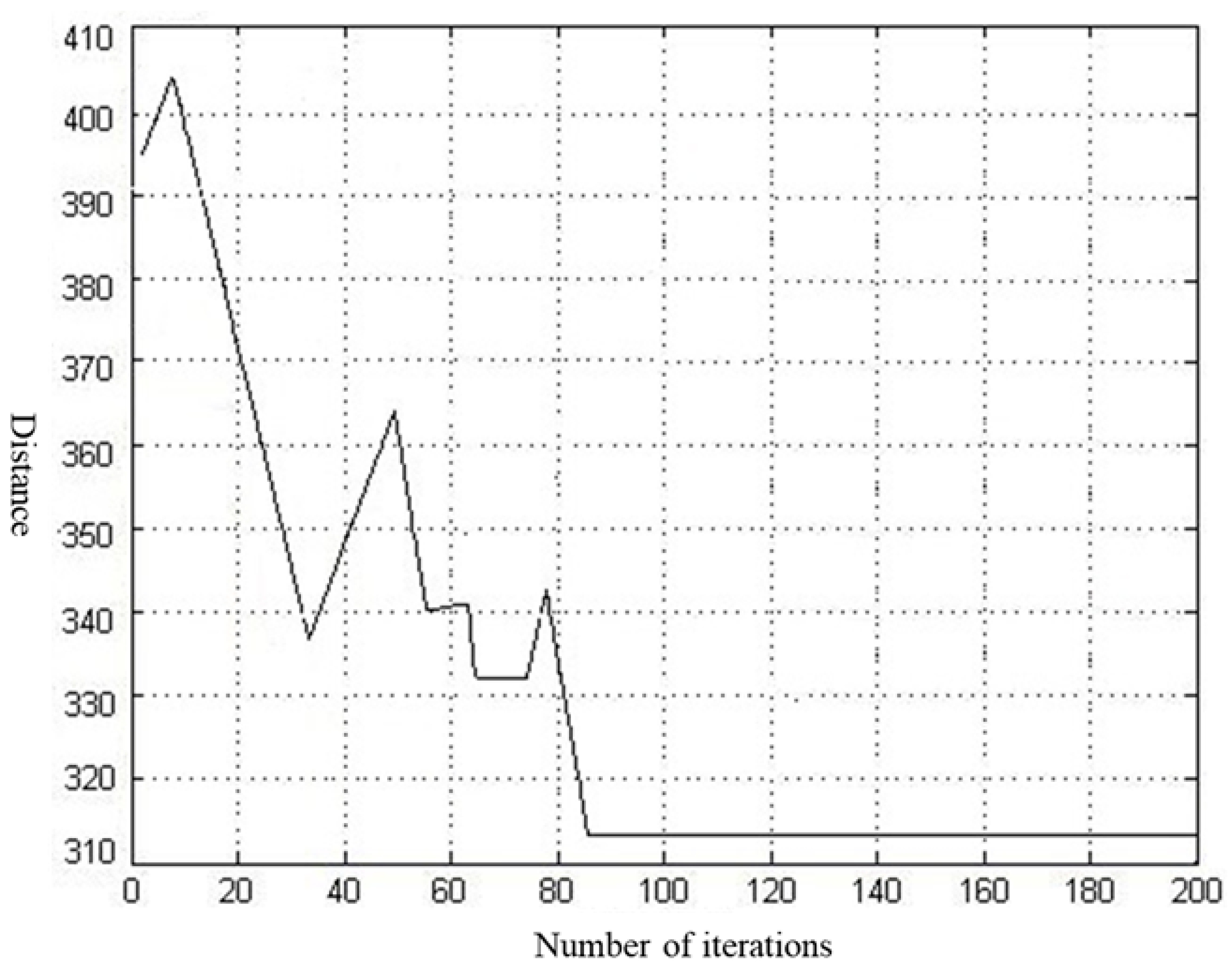
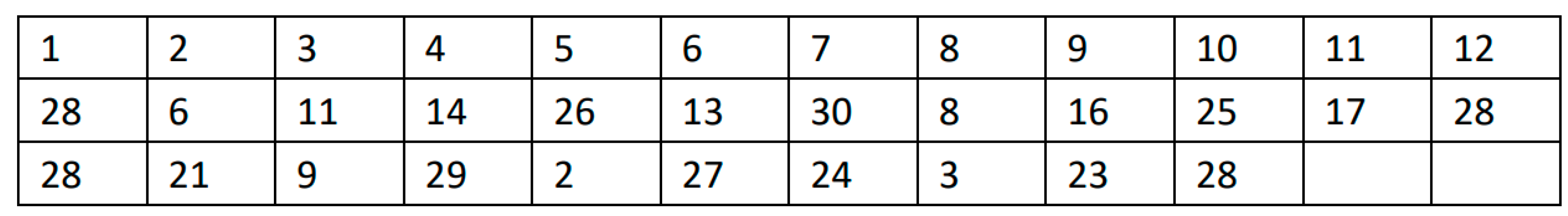
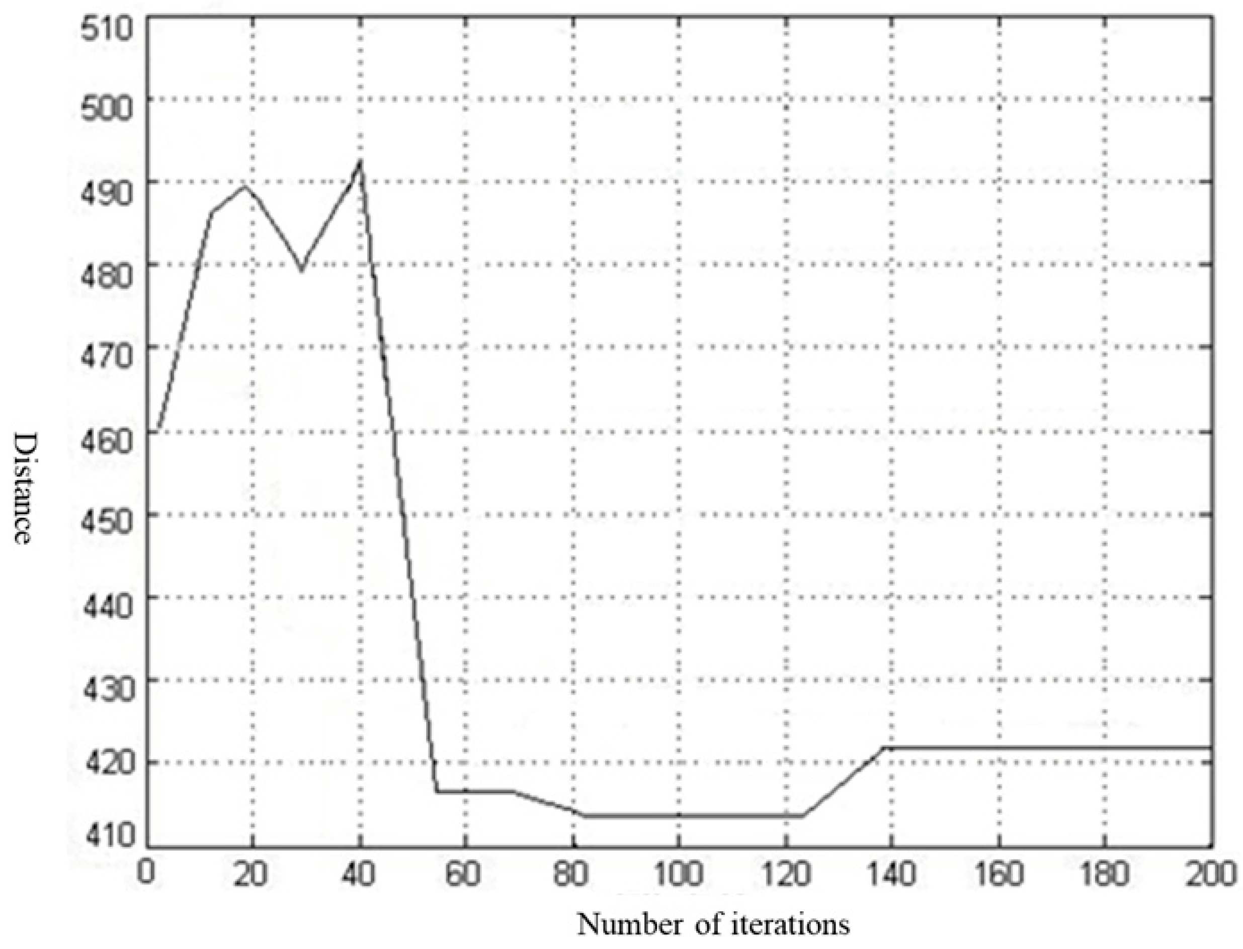
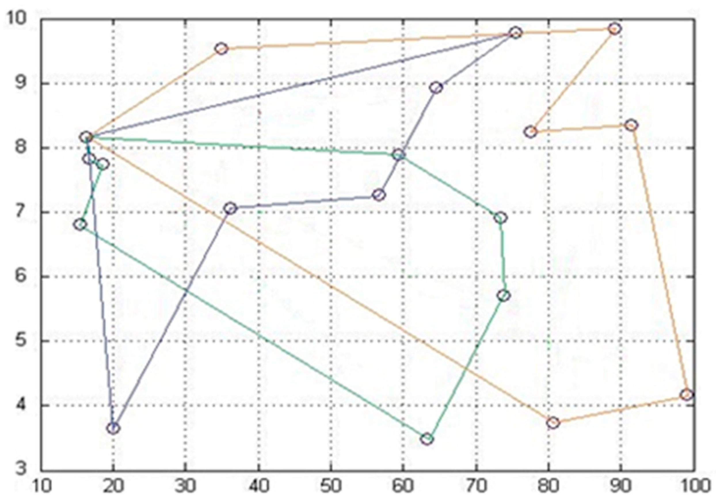
3.2.2. Vehicle Routing Results

The results of multiple experiments are shown in Figure 10 and Figure 11. The optimization results for the agricultural waste transportation route are shown in Figure 12 (as mentioned in the previous section, the processing station is located at position 28, so the starting point and endpoint are also set to 28). As shown in Figure 13, the results converged after 95 iterations, demonstrating good convergence performance. The distance of the transportation route decreases from the initial 351.24 km to 268.17 km.

Collecting APW from 19 temporary storage locations requires two vehicles, with an optimal transportation cost of CNY 798.4. The transportation route for the first vehicle is 28–6–11–14–26–17–23–25–9–21–28; the transportation route for the second vehicle is 28–16–3–24–29–2–27–8–30–13–28.

The optimal route optimization results for the APW when the vehicle’s load capacity is 13 t are shown in Figure 12 and Figure 13.

From Figure 13, we can see that the optimal route distance is 312.10 km, and the optimal transportation cost at this point is CNY 983.5.

As shown in Figure 14, the transport route for the first vehicle is 28–6–11–14–26–13–30–8–16–25–17–28; the transport route for the second vehicle is 28–21–9–29–2–27–24–3–23–28.

The APW’s optimal route results when the vehicle load was 10 t are shown in Figure 15 and Figure 16.

From Figure 15, we can see that the optimal route distance for vehicle transportation is 422.73 km, and the optimal transportation cost is CNY 1147.8.

The transport routes for the first, second, and third vehicles are 28–6–11–14–13–16–3–25–28, 28–29–9–23–17–26–28, and 28–21–2–24–27–8–30–28, respectively.

From the above analysis, it can be observed that the load capacity of a vehicle affects the number of transport vehicles, optimal transport route, and optimal cost. By comparison, it can be observed that choosing a vehicle with a load capacity of 12 t results in the lowest transport cost of CNY 798.4, as shown in

Table 5. Impact of APW vehicle load changes on results.

Vehicle Load Capacity (t)	Number of Vehicles	Distance Before Optimization (km)	Optimized Optimal Distance (km)	Cost Before Optimization (CNY)	Optimized Cost (CNY)
12	2	351.24	268.17	1013.1	798.4
13	2	395.72	312.10	1137.4	983.5
10	3	461.28	422.73	1404.8	1147.8

.

The vehicle path optimization results (Table 5) indicate that the 12 t load scheme achieves optimal performance in terms of both transportation distance (268.17 km) and cost (CNY 798.4). Further analysis reveals that this scheme optimizes vehicle scheduling by assigning Vehicle 1 to serve 11 sites and Vehicle 2 to serve 8 sites, thereby increasing the actual load factor to 92%, an improvement of 18 percentage points compared to the initial path. Based on a diesel vehicle emission factor of 0.25 kg/km, the carbon emissions amount to 67.04 kg, a reduction of 23.7% compared to the initial route (87.81 kg). This confirms the dual advantages of the ant colony algorithm in reducing operational costs and environmental impact, providing an economical and environmentally friendly transportation model for rural waste recycling.

Therefore, in actual situations, in order to reduce the transportation costs of recycled APW, it is necessary to select the appropriate load-bearing vehicle type for recycling transportation based on the location of the APW temporary storage site and the amount of APW generated at each temporary storage site.

4. Discussion

APW pollution is severe, widely distributed, and occurs unpredictably. Combined with the inadequate treatment facilities in rural areas, this poses significant challenges to the environment and public health. To address this challenge, we developed a two-stage site selection model for APW recycling network facilities based on IA and AHP/fuzzy logic and conducted simulation studies. For the APW recycling vehicle transportation problem, we constructed an APW vehicle scheduling path optimization model and used the ACA to solve for the optimal results, as shown in

Table 6. Research modules, methods, and content.

Research Module	Research Methods	Research Content
Temporary Storage Site Selection	Immune Algorithm (IA) and Set Covering Model	With the goal of minimizing the number of facilities, input 110 production point coordinates and yields, and output 16–19 candidate temporary storage points
Treatment Plant Site Selection	AHP and FCEM	Screen the optimal sites from the candidate sites, input geographical/economic/environmental constraints, and output the coordinates of the processing stations
Path Optimization	Ant Colony Algorithm (ACA) and Vehicle Scheduling Model	Plan transportation routes based on site distribution, input load/distance costs, and output the lowest-cost vehicle route plan

. This study aims to provide a relevant decision-making basis for the site selection and path optimization of APW recycling facilities, making the recycling and treatment of APW more scientific, reasonable, and effective.

The results of this study are consistent with the existing literature in several respects. For example, Wang et al. pointed out that the resource utilization of APW in China is still in its infancy, with high resource utilization difficulties and weak infrastructure in rural areas, which aligns with the issues mentioned in this study regarding APW recycling and the insufficient infrastructure in rural areas [78]. In terms of recycling network planning, Ayyildiz and Erdogan also emphasized the importance of site layout and suggested combining qualitative and quantitative analysis methods for site selection [79], which aligns with the use of multiple methods for site optimization. However, there are some inconsistencies between the results of this study and the existing literature. In terms of research methods for recycling network planning, some studies primarily used mixed-integer linear programming methods to establish optimization models [14,80], while this study innovatively combines the IA and AHP/fuzzy to construct a two-stage site selection model and uses the ACA to solve vehicle scheduling path optimization problems. A comprehensive application of this method is relatively uncommon in the literature.

This study has certain significance. Theoretical level: Establishing a recycling network for APW and strengthening its circular utilization is an inevitable requirement for achieving ecological civilization and ecological security. Establishing a recycling logistics network for APW facilitates the exploration of the intrinsic laws of reverse logistics and agricultural ecology theory, and it deepens research on the selection of recycling facilities and vehicle scheduling routes for APW. Research on the selection and layout of sites and the optimization of vehicle dispatch routes in the APW recycling network provides theoretical guidance for the planning of APW recycling networks. Practical level: Research on the planning of APW recycling networks helps guide farmers to properly handle agricultural production waste, reduce environmental pollution, and alleviate the situation of relative resource shortages in China. A scientific and reasonable layout of APW recycling facilities can improve rural environmental quality, thereby enhancing the living environment of rural households. Optimization of vehicle scheduling and recycling routes can enhance the operational and management efficiency of APW recycling in rural areas, reduce recycling transportation costs, and provide scientific decision-making basis for the optimization design of APW recycling networks. The optimization mechanism of this study further reveals three generalizable practical experiences: first, prioritizing site layout in high-yield APW areas such as coordinates x ∈ [15, 30] can reduce transportation costs by 23%; second, standardizing the use of 12-ton vehicles instead of 13-ton vehicles can save an average of CNY 67,000 in annual operating costs; third, promoting the single-point wide coverage model of site 8 can reduce facility investment in remote areas by 30%. Policy-wise: based on the research results, measures such as strengthening infrastructure construction, promoting optimized models, providing policy support, and enhancing supervision and evaluation should be implemented.

Research on the optimized design of APW recycling networks, whether theoretical or empirical, warrants further exploration. This study represents only an initial effort in this area, focusing solely on the optimized selection of collection and storage sites, processing stations, and vehicle scheduling routes within APW recycling networks. However, additional studies need to be conducted. Key areas requiring further research and the limitations of this study are outlined below.

(1)

Selection of APW recycling temporary storage and processing stations: In constructing the set coverage model, this study assumes that the construction cost of APW recycling temporary storage sites is sufficiently large compared with other costs. Without this assumption, the constructed model may not be able to solve the selection problem of temporary storage sites for APW recycling. Additionally, for the selected evaluation indicator system constructed for processing station site selection, many qualitative factors need to be considered in real-world scenarios. This study selects four indicators: infrastructure, natural conditions, operational characteristics, and economic and environmental effects. Four core indicators were selected, primarily based on their systematic nature and suitability for the field. In terms of systematicity, the four categories of indicators cover the entire lifecycle of the recycling network: infrastructure (transportation conditions, land costs) forms the physical foundation for logistics efficiency; natural conditions (topography, weather) determine the feasibility of construction and operational stability; operational characteristics (matching degree of waste properties, service response speed, logistics costs) ensure the network aligns with the spatio-temporal characteristics of agricultural production; and economic and environmental effects (disruption to residents’ lives, ecological impact) ensure sustainable development. In terms of domain-specific relevance, the indicators are designed to align with the unique characteristics of agricultural production waste: infrastructure indicators address the current weaknesses in rural infrastructure (e.g., high-weight transportation assessments), natural condition indicators mitigate risks associated with agricultural environmental sensitivity (e.g., wind direction’s impact on pollution dispersion), operational characteristic indicators address the spatial and temporal dispersion of waste (e.g., seasonal recycling demands), and economic and environmental indicators balance costs with social acceptability. More indicators should be considered in future research.

(2)

Selection of optimization objectives: The model constructed for APW recycling and temporary storage sites only selected a single optimization objective and did not establish a multi-objective model. For example, the social and environmental impacts of temporary APW storage sites can also be considered.

(3)

Data acquisition: Because of the difficulty in obtaining data on APW generation points, a numerical simulation was used in this study. Although the effectiveness of the established model and algorithm was verified to a certain extent, efforts should be made to obtain and verify actual data.

(4)

Algorithm selection: In this study, the IA was used to solve the treatment plant location problem, and the ACA was used to solve the vehicle scheduling path optimization model. These results indicate that the constructed model was effective and reasonable. However, whether other algorithms (such as genetic algorithms or simulated annealing algorithms) can solve the APW recycling temporary storage facility and vehicle scheduling path optimization models remains to be further studied. However, future research could systematically introduce other high-performance heuristic or meta-heuristic algorithms, such as genetic algorithms (GAs), simulated annealing (SA) algorithms, and particle swarm optimization (PSO), for comparative experiments. By designing a fair comparison environment, such as using the same dataset, parameter settings, and computational platform, and conducting a comprehensive evaluation of key metrics such as optimal solution quality, average solution quality, computation time, convergence speed, and algorithm stability, we can more objectively reveal the relative advantages and applicable scenarios of different algorithms in APW recycling network optimization problems, providing a more robust basis for algorithm selection in practice.

5. Conclusions

This paper investigates the optimization of the recycling network for APW from two perspectives: the selection of optimal locations for temporary storage sites and processing stations as well as the optimization of vehicle scheduling and routes for APW recycling. The main innovative research findings are as follows:

First, a two-stage site selection model was developed for APW recycling temporary storage facilities and processing stations. With the objective of minimizing the number of facilities, a set coverage site selection model was constructed. In the first stage, the immune algorithm was used to determine the initial locations of the temporary storage facilities, and the model’s effectiveness was validated through numerical simulation analysis. Based on this, an indicator system for the selection of APW recycling processing stations was established. In the second stage, the AHP and FCEM were used to precisely select the locations of the recycling processing stations, ultimately identifying the optimal locations for the APW recycling processing stations. Second, to address the transportation issue of APW recycling vehicles, a vehicle scheduling path optimization model was constructed for APW. Considering the characteristics of APW, such as dispersed generation locations and large generation volumes, the ACA was used to solve the constructed model, and the optimal recycling vehicle scheduling plan and detailed transportation path plan for each vehicle were finally provided. Through the above research, the effectiveness of the model was verified, and the recycling transportation costs of APW were effectively reduced.

The collection and transportation of APW are critical components in the design of a recycling network, ensuring that the APW generated in various regions can be processed in a reasonable and effective manner. Based on this, this study investigated the optimization of site selection for APW recycling storage facilities and processing stations, as well as the scheduling and optimization of recycling transportation vehicles.

(1)

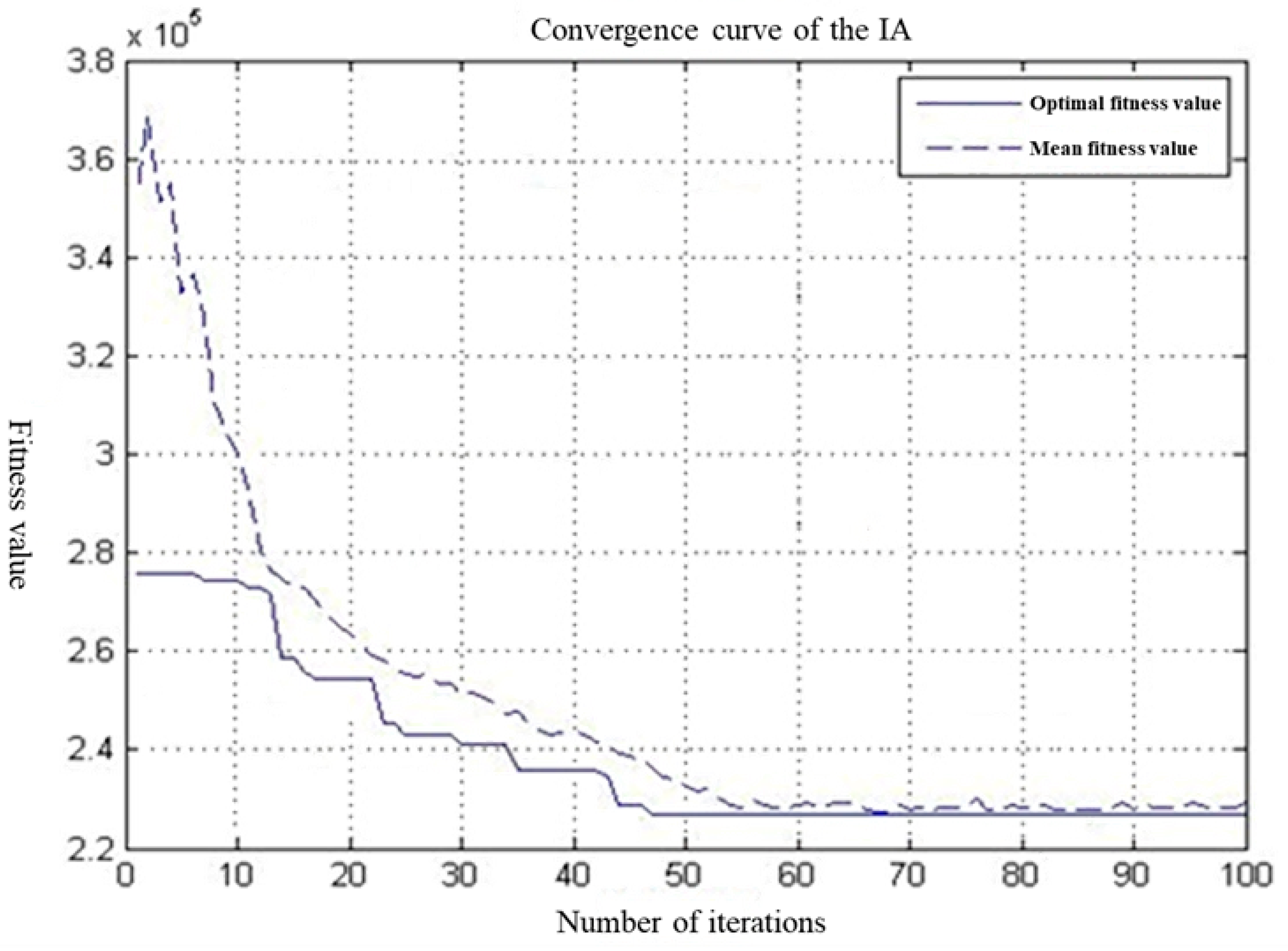
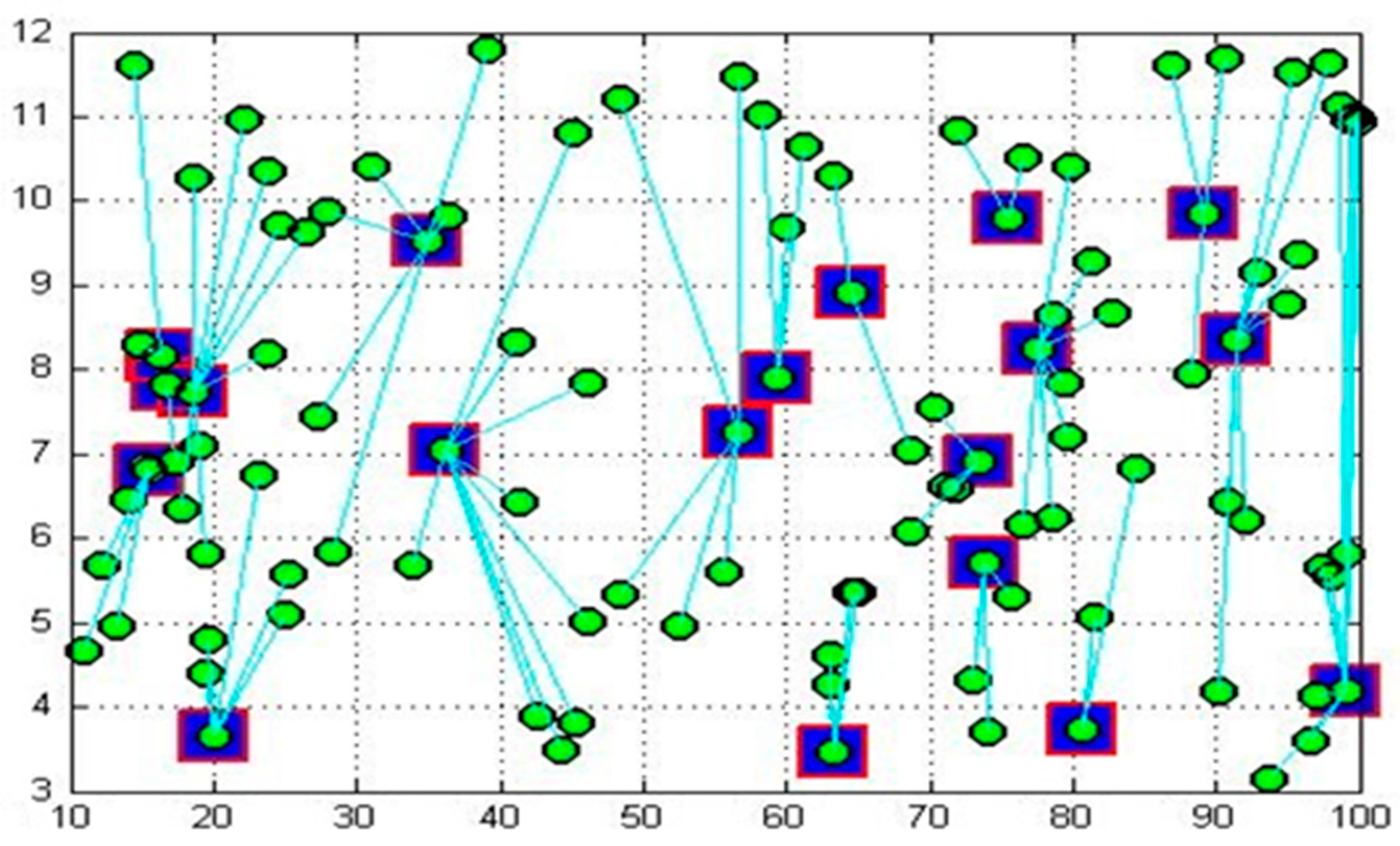
Given the characteristics of APW mentioned earlier, facility construction costs typically need to be considered during the site selection process. The objective was to minimize the number of facilities, and a set coverage site selection model was constructed. We randomly selected 110 APW generation points. These 110 APW generation points were used as the objects of the recycling temporary storage facility site selection study, and simulation research was conducted. The IA method was used to solve the constructed model, and based on the different quantities of APW generated, different numbers and locations of temporary storage facilities for APW recycling were selected.

(2)

The optimal location for the recycling treatment station was precisely selected from the selected temporary storage sites. During the precise site selection process, four key indicators were considered: infrastructure, the natural environment, operational characteristics, and economic and environmental impacts. An evaluation indicator system for the precise selection of APW treatment station locations was established, and the analytic hierarchy process (AHP) and fuzzy comprehensive evaluation method were employed to precisely select the optimal location for the recycling treatment station.

(3)

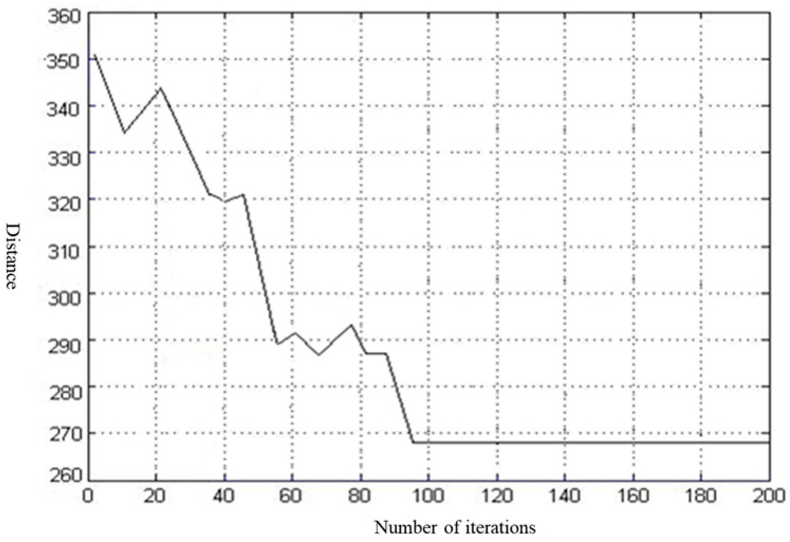
A scheduling and path optimization model suitable for APW recycling transport vehicles was constructed and solved using the ACA. Finally, the optimal recycling vehicle scheduling plan and detailed transport path plan for each vehicle were designed. Through this research, the infrastructure construction and transport costs of APW recycling were effectively reduced. For example, when the load capacity of the collected vehicle is 12 tons, the distance of the transportation route decreases from the initial 351.24 km to 268.17 km, a reduction of 23.65%.

References

1. Qu, L.; Li, Y.; Yang, F.; Ma, L.; Chen, Z. Assessing Sustainable Transformation and Development Strategies for Gully Agricultural Production: A Case Study in the Loess Plateau of China. Environ. Impact Assess. Rev. 2024, 104, 107325. [Google Scholar] [CrossRef]
2. Babu, S.; Singh Rathore, S.; Singh, R.; Kumar, S.; Singh, V.K.; Yadav, S.K.; Yadav, V.; Raj, R.; Yadav, D.; Shekhawat, K.; et al. Exploring Agricultural Waste Biomass for Energy, Food and Feed Production and Pollution Mitigation: A Review. Bioresour. Technol. 2022, 360, 127566. [Google Scholar] [CrossRef]
3. Capanoglu, E.; Nemli, E.; Tomas-Barberan, F. Novel Approaches in the Valorization of Agricultural Wastes and Their Applications. J. Agric. Food Chem. 2022, 70, 6787–6804. [Google Scholar] [CrossRef] [PubMed]
4. Sonu; Rani, G.M.; Pathania, D.; Abhimanyu; Umapathi, R.; Rustagi, S.; Huh, Y.S.; Gupta, V.K.; Kaushik, A.; Chaudhary, V. Agro-Waste to Sustainable Energy: A Green Strategy of Converting Agricultural Waste to Nano-Enabled Energy Applications. Sci. Total Environ. 2023, 875, 162667. [Google Scholar] [CrossRef] [PubMed]
5. Wei, J.; Liang, G.; Alex, J.; Zhang, T.; Ma, C. Research Progress of Energy Utilization of Agricultural Waste in China: Bibliometric Analysis by Citespace. Sustainability 2020, 12, 812. [Google Scholar] [CrossRef]
6. Safieddin Ardebili, S.M. Green Electricity Generation Potential from Biogas Produced by Anaerobic Digestion of Farm Animal Waste and Agriculture Residues in Iran. Renew. Energy 2020, 154, 29–37. [Google Scholar] [CrossRef]
7. Amen, R.; Hameed, J.; Albashar, G.; Kamran, H.W.; Hassan Shah, M.U.; Zaman, M.K.U.; Mukhtar, A.; Saqib, S.; Ch, S.I.; Ibrahim, M.; et al. Modelling the Higher Heating Value of Municipal Solid Waste for Assessment of Waste-to-Energy Potential: A Sustainable Case Study. J. Clean. Prod. 2021, 287, 125575. [Google Scholar] [CrossRef]
8. Sharma, B.; Vaish, B.; Monika; Singh, U.K.; Singh, P.; Singh, R.P. Recycling of Organic Wastes in Agriculture: An Environmental Perspective. Int. J. Environ. Res. 2019, 13, 409–429. [Google Scholar] [CrossRef]
9. Sarfaraz, Q.; da Silva, L.S.; Drescher, G.L.; Zafar, M.; Severo, F.F.; Kokkonen, A.; Dal Molin, G.; Shafi, M.I.; Shafique, Q.; Solaiman, Z.M. Characterization and Carbon Mineralization of Biochars Produced from Different Animal Manures and Plant Residues. Sci. Rep. 2020, 10, 955. [Google Scholar] [CrossRef]
10. Shi, Q.; Ren, H.; Ma, X.; Xiao, Y. Site Selection of Construction Waste Recycling Plant. J. Clean. Prod. 2019, 227, 532–542. [Google Scholar] [CrossRef]
11. Nuhu, S.K.; Manan, Z.A.; Wan Alwi, S.R.; Md Reba, M.N. Integrated Modelling Approach for an Eco-Industrial Park Site Selection. J. Clean. Prod. 2022, 368, 133141. [Google Scholar] [CrossRef]
12. Liu, J.; Xiao, Y.; Wang, D.; Pang, Y. Optimization of Site Selection for Construction and Demolition Waste Recycling Plant Using Genetic Algorithm. Neural Comput. Appl. 2019, 31, 233–245. [Google Scholar] [CrossRef]
13. Abdel-Basset, M.; Gamal, A.; Chakrabortty, R.K.; Ryan, M. A New Hybrid Multi-Criteria Decision-Making Approach for Location Selection of Sustainable Offshore Wind Energy Stations: A Case Study. J. Clean. Prod. 2021, 280, 124462. [Google Scholar] [CrossRef]
14. Shao, M.; Han, Z.; Sun, J.; Xiao, C.; Zhang, S.; Zhao, Y. A Review of Multi-Criteria Decision Making Applications for Renewable Energy Site Selection. Renew. Energy 2020, 157, 377–403. [Google Scholar] [CrossRef]
15. Bao, Z.; Lu, W. Developing Efficient Circularity for Construction and Demolition Waste Management in Fast Emerging Economies: Lessons Learned from Shenzhen, China. Sci. Total Environ. 2020, 724, 138264. [Google Scholar] [CrossRef]
16. Ghaffar, S.H.; Burman, M.; Braimah, N. Pathways to Circular Construction: An Integrated Management of Construction and Demolition Waste for Resource Recovery. J. Clean. Prod. 2020, 244, 118710. [Google Scholar] [CrossRef]
17. Mustafa, H.M.; Hayder, G. Recent Studies on Applications of Aquatic Weed Plants in Phytoremediation of Wastewater: A Review Article. Ain Shams Eng. J. 2021, 12, 355–365. [Google Scholar] [CrossRef]
18. Attrah, M.; Elmanadely, A.; Akter, D.; Rene, E.R. A Review on Medical Waste Management: Treatment, Recycling, and Disposal Options. Environments 2022, 9, 146. [Google Scholar] [CrossRef]
19. Mei, X.; Hao, H.; Sun, Y.; Wang, X.; Zhou, Y. Optimization of Medical Waste Recycling Network Considering Disposal Capacity Bottlenecks under a Novel Coronavirus Pneumonia Outbreak. Environ. Sci. Pollut. Res. 2022, 29, 79669–79687. [Google Scholar] [CrossRef]
20. Liu, S.; Zhang, J.; Niu, B.; Liu, L.; He, X. A Novel Hybrid Multi-Criteria Group Decision-Making Approach with Intuitionistic Fuzzy Sets to Design Reverse Supply Chains for COVID-19 Medical Waste Recycling Channels. Comput. Ind. Eng. 2022, 169, 108228. [Google Scholar] [CrossRef]
21. Liu, M.; Wen, J.; Feng, Y.; Zhang, L.; Wu, J.; Wang, J.; Yang, X. A Benefit Evaluation for Recycling Medical Plastic Waste in China Based on Material Flow Analysis and Life Cycle Assessment. J. Clean. Prod. 2022, 368, 133033. [Google Scholar] [CrossRef]
22. Le, H.T.; Quoc, K.L.; Nguyen, T.A.; Dang, K.T.; Vo, H.K.; Luong, H.H.; Le Van, H.; Gia, K.H.; Cao Phu, L.V.; Nguyen Truong Quoc, D.; et al. Medical-Waste Chain: A Medical Waste Collection, Classification and Treatment Management by Blockchain Technology. Computers 2022, 11, 113. [Google Scholar] [CrossRef]
23. Yoon, C.-W.; Kim, M.-J.; Park, Y.-S.; Jeon, T.-W.; Lee, M.-Y. A Review of Medical Waste Management Systems in the Republic of Korea for Hospital and Medical Waste Generated from the COVID-19 Pandemic. Sustainability 2022, 14, 3678. [Google Scholar] [CrossRef]
24. Govindan, K.; Nosrati-Abarghooee, S.; Nasiri, M.M.; Jolai, F. Green Reverse Logistics Network Design for Medical Waste Management: A Circular Economy Transition through Case Approach. J. Environ. Manag. 2022, 322, 115888. [Google Scholar] [CrossRef]
25. Tushar, S.R.; Alam, M.D.F.B.; Bari, A.B.M.M.; Karmaker, C.L. Assessing the Challenges to Medical Waste Management during the COVID-19 Pandemic: Implications for the Environmental Sustainability in the Emerging Economies. Socioecon. Plann. Sci. 2023, 87, 101513. [Google Scholar] [CrossRef]
26. Yu, H.; Sun, X.; Solvang, W.D.; Zhao, X. Reverse Logistics Network Design for Effective Management of Medical Waste in Epidemic Outbreaks: Insights from the Coronavirus Disease 2019 (COVID-19) Outbreak in Wuhan (China). Int. J. Environ. Res. Public. Health 2020, 17, 1770. [Google Scholar] [CrossRef]
27. Aboelmaged, M. E-Waste Recycling Behaviour: An Integration of Recycling Habits into the Theory of Planned Behaviour. J. Clean. Prod. 2021, 278, 124182. [Google Scholar] [CrossRef]
28. Liu, K.; Tan, Q.; Yu, J.; Wang, M. A Global Perspective on E-Waste Recycling. Circ. Econ. 2023, 2, 100028. [Google Scholar] [CrossRef]
29. Vuppaladadiyam, S.S.V.; Thomas, B.S.; Kundu, C.; Vuppaladadiyam, A.K.; Duan, H.; Bhattacharya, S. Can E-Waste Recycling Provide a Solution to the Scarcity of Rare Earth Metals? An Overview of e-Waste Recycling Methods. Sci. Total Environ. 2024, 924, 171453. [Google Scholar] [CrossRef]
30. Dhir, A.; Koshta, N.; Goyal, R.K.; Sakashita, M.; Almotairi, M. Behavioral Reasoning Theory (BRT) Perspectives on E-Waste Recycling and Management. J. Clean. Prod. 2021, 280, 124269. [Google Scholar] [CrossRef]
31. Wang, Z.; Huo, J. Do Government Intervention Measures Promote E-Waste Recycling in China? J. Environ. Manag. 2023, 342, 118138. [Google Scholar] [CrossRef] [PubMed]
32. Lovrak, A.; Pukšec, T.; Duić, N. A Geographical Information System (GIS) Based Approach for Assessing the Spatial Distribution and Seasonal Variation of Biogas Production Potential from Agricultural Residues and Municipal Biowaste. Appl. Energy 2020, 267, 115010. [Google Scholar] [CrossRef]
33. Yan, B.; Li, Y.; Qin, Y.; Shi, W.; Yan, J. Spatial-Temporal Distribution of Biogas Production from Agricultural Waste per Capita in Rural China and Its Correlation with Ground Temperature. Sci. Total Environ. 2022, 817, 152987. [Google Scholar] [CrossRef]
34. Cowie, P.; Townsend, L.; Salemink, K. Smart Rural Futures: Will Rural Areas Be Left behind in the 4th Industrial Revolution? J. Rural Stud. 2020, 79, 169–176. [Google Scholar] [CrossRef] [PubMed]
35. Prus, P.; Sikora, M. The Impact of Transport Infrastructure on the Sustainable Development of the Region—Case Study. Agriculture 2021, 11, 279. [Google Scholar] [CrossRef]
36. Xiao, D.; An, S.; Cai, H.; Wang, J.; Cai, H. An Optimization Model for Electric Vehicle Charging Infrastructure Planning Considering Queuing Behavior with Finite Queue Length. J. Energy Storage 2020, 29, 101317. [Google Scholar] [CrossRef]
37. Zhang, H.; Zhang, Q.; Ma, L.; Zhang, Z.; Liu, Y. A Hybrid Ant Colony Optimization Algorithm for a Multi-Objective Vehicle Routing Problem with Flexible Time Windows. Inf. Sci. 2019, 490, 166–190. [Google Scholar] [CrossRef]
38. Fu, Y.; Li, H.; Huang, M.; Xiao, H. Bi-Objective Modeling and Optimization for Stochastic Two-Stage Open Shop Scheduling Problems in the Sharing Economy. IEEE Trans. Eng. Manag. 2023, 70, 3395–3409. [Google Scholar] [CrossRef]
39. Peng, X.; Jiang, Y.; Chen, Z.; Osman, A.I.; Farghali, M.; Rooney, D.W.; Yap, P.-S. Recycling Municipal, Agricultural and Industrial Waste into Energy, Fertilizers, Food and Construction Materials, and Economic Feasibility: A Review. Environ. Chem. Lett. 2023, 21, 765–801. [Google Scholar] [CrossRef]
40. Sikiru, S.; Abioye, K.J.; Adedayo, H.B.; Adebukola, S.Y.; Soleimani, H.; Anar, M. Technology Projection in Biofuel Production Using Agricultural Waste Materials as a Source of Energy Sustainability: A Comprehensive Review. Renew. Sustain. Energy Rev. 2024, 200, 114535. [Google Scholar] [CrossRef]
41. Damian, C.S.; Devarajan, Y.; Jayabal, R. A Comprehensive Review of the Resource Efficiency and Sustainability in Biofuel Production from Industrial and Agricultural Waste. J. Mater. Cycles Waste Manag. 2024, 26, 1264–1276. [Google Scholar] [CrossRef]
42. Ufitikirezi, J.D.D.M.; Filip, M.; Ghorbani, M.; Zoubek, T.; Olšan, P.; Bumbálek, R.; Strob, M.; Bartoš, P.; Umurungi, S.N.; Murindangabo, Y.T.; et al. Agricultural Waste Valorization: Exploring Environmentally Friendly Approaches to Bioenergy Conversion. Sustainability 2024, 16, 3617. [Google Scholar] [CrossRef]
43. Atinkut, H.B.; Yan, T.; Zhang, F.; Qin, S.; Gai, H.; Liu, Q. Cognition of Agriculture Waste and Payments for a Circular Agriculture Model in Central China. Sci. Rep. 2020, 10, 10826. [Google Scholar] [CrossRef]
44. Zhang, H.G.; Tang, X.Y. Study on Optimized Combination and Utilization Model of Agricultural and Animal Husbandry Resources in Mountain Ecotone. IOP Conf. Ser. Earth Environ. Sci. 2019, 346, 012031. [Google Scholar] [CrossRef]
45. Han, R.; Huo-Gen, W. N2N Regional Circular Agriculture Model in China: A Case Study of Luofang Biogas Project. Cogent Food Agric. 2023, 9, 2222563. [Google Scholar] [CrossRef]
46. Zhou, K.; Li, Y.; Tang, Y.; Yang, Y.; Tian, G.; Liu, B.; Bian, B.; He, C. A New Scheme for Low-Carbon Recycling of Urban and Rural Organic Waste Based on Carbon Footprint Assessment: A Case Study in China. Npj Sustain. Agric. 2024, 2, 9. [Google Scholar] [CrossRef]
47. Chen, L.; Dong, T.; Peng, J.; Ralescu, D. Uncertainty Analysis and Optimization Modeling with Application to Supply Chain Management: A Systematic Review. Mathematics 2023, 11, 2530. [Google Scholar] [CrossRef]
48. Rokbani, N.; Kumar, R.; Abraham, A.; Alimi, A.M.; Long, H.V.; Priyadarshini, I.; Son, L.H. Bi-Heuristic Ant Colony Optimization-Based Approaches for Traveling Salesman Problem. Soft Comput. 2021, 25, 3775–3794. [Google Scholar] [CrossRef]
49. Wang, Y.; Han, Z. Ant Colony Optimization for Traveling Salesman Problem Based on Parameters Optimization. Appl. Soft Comput. 2021, 107, 107439. [Google Scholar] [CrossRef]
50. Wu, L.; Huang, X.; Cui, J.; Liu, C.; Xiao, W. Modified Adaptive Ant Colony Optimization Algorithm and Its Application for Solving Path Planning of Mobile Robot. Expert Syst. Appl. 2023, 215, 119410. [Google Scholar] [CrossRef]
51. Koul, B.; Yakoob, M.; Shah, M.P. Agricultural Waste Management Strategies for Environmental Sustainability. Environ. Res. 2022, 206, 112285. [Google Scholar] [CrossRef]
52. Agapkin, A.M.; Makhotina, I.A.; Ibragimova, N.A.; Goryunova, O.B.; Izembayeva, A.K.; Kalachev, S.L. The Problem of Agricultural Waste and Ways to Solve It. IOP Conf. Ser. Earth Environ. Sci. 2022, 981, 022009. [Google Scholar] [CrossRef]
53. Maraveas, C. Production of Sustainable and Biodegradable Polymers from Agricultural Waste. Polymers 2020, 12, 1127. [Google Scholar] [CrossRef]
54. Jeong, J.S.; García-Moruno, L.; Hernández-Blanco, J. A Site Planning Approach for Rural Buildings into a Landscape Using a Spatial Multi-Criteria Decision Analysis Methodology. Land Use Policy 2013, 32, 108–118. [Google Scholar] [CrossRef]
55. Agramanisti Azdy, R.; Darnis, F. Use of Haversine Formula in Finding Distance Between Temporary Shelter and Waste End Processing Sites. J. Phys. Conf. Ser. 2020, 1500, 012104. [Google Scholar] [CrossRef]
56. Albahri, O.S.; Zaidan, A.A.; Zaidan, B.B.; Albahri, A.S.; Mohsin, A.H.; Mohammed, K.I.; Alsalem, M.A. New mHealth Hospital Selection Framework Supporting Decentralised Telemedicine Architecture for Outpatient Cardiovascular Disease-Based Integrated Techniques: Haversine-GPS and AHP-VIKOR. J. Ambient Intell. Humaniz. Comput. 2022, 13, 219–239. [Google Scholar] [CrossRef]
57. Zhang, Y.; Schaap, M.G.; Wei, Z. Development of Hierarchical Ensemble Model and Estimates of Soil Water Retention with Global Coverage. Geophys. Res. Lett. 2020, 47, e2020GL088819. [Google Scholar] [CrossRef]
58. Li, L.; Lin, Q.; Li, K.; Ming, Z. Vertical Distance-Based Clonal Selection Mechanism for the Multiobjective Immune Algorithm. Swarm Evol. Comput. 2021, 63, 100886. [Google Scholar] [CrossRef]
59. Yu, X.; Tian, X. A Fault Detection Algorithm for Pipeline Insulation Layer Based on Immune Neural Network. Int. J. Press. Vessels Pip. 2022, 196, 104611. [Google Scholar] [CrossRef]
60. Aslan, S.; Rohacs, D.; Yıldız, M.; Kale, U. A Three-Dimensional UCAV Path Planning Approach Based on Immune Plasma Algorithm. Int. J. Comput. Intell. Syst. 2023, 16, 112. [Google Scholar] [CrossRef]
61. Tang, C.; Todo, Y.; Ji, J.; Lin, Q.; Tang, Z. Artificial Immune System Training Algorithm for a Dendritic Neuron Model. Knowl.-Based Syst. 2021, 233, 107509. [Google Scholar] [CrossRef]
62. Kuikka, V.; Aalto, H.; Ijäs, M.; Kaski, K.K. Efficiency of Algorithms for Computing Influence and Information Spreading on Social Networks. Algorithms 2022, 15, 262. [Google Scholar] [CrossRef]
63. Forestal, R.L.; Pi, S.-M. A Hybrid Approach Based on ELECTRE III-Genetic Algorithm and TOPSIS Method for Selection of Optimal COVID-19 Vaccines. J. Multi-Criteria Decis. Anal. 2022, 29, 80–91. [Google Scholar] [CrossRef] [PubMed]
64. Li, K.; Luo, J.; Hu, Y.; Li, S. A Novel Multi-Strategy DE Algorithm for Parameter Optimization in Support Vector Machine. J. Intell. Inf. Syst. 2020, 54, 527–543. [Google Scholar] [CrossRef]
65. Spampinato, A.G.; Scollo, R.A.; Cutello, V.; Pavone, M. Random Search Immune Algorithm for Community Detection. Soft Comput. 2023, 27, 8061–8090. [Google Scholar] [CrossRef]
66. Holland, J.H. Adaptation in Natural and Artificial Systems: An Introductory Analysis with Applications to Biology, Control, and Artificial Intelligence; The MIT Press: Cambridge, MA, USA, 1992; ISBN 978-0-262-27555-2. [Google Scholar]
67. Kirkpatrick, S.; Gelatt, C.D.; Vecchi, M.P. Optimization by Simulated Annealing. Science 1983, 220, 671–680. [Google Scholar] [CrossRef]
68. Zhang, Y.; Shang, K. Evaluation of Mine Ecological Environment Based on Fuzzy Hierarchical Analysis and Grey Relational Degree. Environ. Res. 2024, 257, 119370. [Google Scholar] [CrossRef]
69. Wu, X.; Hu, F. Analysis of Ecological Carrying Capacity Using a Fuzzy Comprehensive Evaluation Method. Ecol. Indic. 2020, 113, 106243. [Google Scholar] [CrossRef]
70. Wu, H.; Sun, X.; Li, D.; Zhao, Y. Research on Learning Evaluation of College Students Based on AHP and Fuzzy Comprehensive Evaluation. Comput. Intell. Neurosci. 2022, 2022, 9160695. [Google Scholar] [CrossRef]
71. Luo, Q.; Wang, H.; Zheng, Y.; He, J. Research on Path Planning of Mobile Robot Based on Improved Ant Colony Algorithm. Neural Comput. Appl. 2020, 32, 1555–1566. [Google Scholar] [CrossRef]
72. Miao, C.; Chen, G.; Yan, C.; Wu, Y. Path Planning Optimization of Indoor Mobile Robot Based on Adaptive Ant Colony Algorithm. Comput. Ind. Eng. 2021, 156, 107230. [Google Scholar] [CrossRef]
73. Yi, N.; Xu, J.; Yan, L.; Huang, L. Task Optimization and Scheduling of Distributed Cyber–Physical System Based on Improved Ant Colony Algorithm. Future Gener. Comput. Syst. 2020, 109, 134–148. [Google Scholar] [CrossRef]
74. Hou, W.; Xiong, Z.; Wang, C.; Chen, H. Enhanced Ant Colony Algorithm with Communication Mechanism for Mobile Robot Path Planning. Robot. Auton. Syst. 2022, 148, 103949. [Google Scholar] [CrossRef]
75. Ataei, P.; Karimi, H.; Hallaj, Z.; Menatizadeh, M. Agricultural Waste Recycling by Farmers: A Behavioral Study. Sustain. Futur. 2025, 9, 100443. [Google Scholar] [CrossRef]
76. Zhang, H.; Ren, Z.; Xin, S.; Liu, S.; Lan, C.; Sun, X. A Scale-Adaptive Positive Selection Algorithm Based on B-Cell Immune Mechanisms for Anomaly Detection. Eng. Appl. Artif. Intell. 2020, 94, 103805. [Google Scholar] [CrossRef]
77. Magalhães, M.T. Spatial Coverage Index for Assessing National and Regional Transportation Infrastructures. J. Transp. Geogr. 2016, 56, 53–61. [Google Scholar] [CrossRef]
78. Wang, J.; Hou, D.; Liu, Z.; Tao, J.; Yan, B.; Liu, Z.; Yang, T.; Su, H.; Tahir, M.H.; Chen, G. Emergy Analysis of Agricultural Waste Biomass for Energy-Oriented Utilization in China: Current Situation and Perspectives. Sci. Total Environ. 2022, 849, 157798. [Google Scholar] [CrossRef]
79. Ayyildiz, E.; Erdogan, M. Literature Analysis of the Location Selection Studies Related to the Waste Facilities within MCDM Approaches. Environ. Sci. Pollut. Res. 2024. [Google Scholar] [CrossRef]
80. Feiz, R.; Metson, G.S.; Wretman, J.; Ammenberg, J. Key Factors for Site-Selection of Biogas Plants in Sweden. J. Clean. Prod. 2022, 354, 131671. [Google Scholar] [CrossRef]
Figure 1. Research framework diagram.
Systems 13 00570 g001
Figure 2. APW recycling network process schematic concept diagram.
Systems 13 00570 g002
Figure 3. Flowchart of the IA.
Systems 13 00570 g003
Figure 4. Site selection evaluation indicator system.
Systems 13 00570 g004
Figure 5. ACA flowchart.
Systems 13 00570 g005
Figure 6. Location and number of APW generation.
Systems 13 00570 g006
Figure 7. Convergence plot of IA.
Systems 13 00570 g007
Figure 8. Map of the location of the 16 recycling staging areas at APW.
Systems 13 00570 g008
Figure 9. Map of the location of the 19 recycling staging areas for APW.
Systems 13 00570 g009
Figure 10. Optimal distance for APW vehicles with a load capacity of 12 t.
Systems 13 00570 g010
Figure 11. Optimal route design for APW vehicles with a load capacity of 12 t.
Systems 13 00570 g011
Figure 12. Optimal distance for APW vehicles with a load capacity of 13 t.
Systems 13 00570 g012
Figure 13. Optimal route design for APW vehicles with a load capacity of 13 t.
Systems 13 00570 g013
Figure 14. APW optimal transport path optimization results II.
Systems 13 00570 g014
Figure 15. Optimal distance for APW vehicles with a load capacity of 10 t.
Systems 13 00570 g015
Figure 16. Optimal route design for APW vehicles with a load capacity of 10 t.
Systems 13 00570 g016