Article

City-Level Road Traffic CO2 Emission Modeling with a Spatial Random Forest Method

1
Faculty of Maritime and Transportation, Ningbo University, Ningbo 315211, China
2
School of Transportation, Southeast University, Nanjing 211189, China
*
Author to whom correspondence should be addressed.
Systems 2025, 13(8), 632; https://doi.org/10.3390/systems13080632
Submission received: 7 May 2025 / Revised: 5 July 2025 / Accepted: 24 July 2025 / Published: 28 July 2025

Abstract

In the era of “carbon dioxide peaking and carbon neutrality”, low-carbon development of road traffic and transportation has now become a rigid demand in China. Considering the fact that socioeconomic and demographic characteristics vary significantly across Chinese cities, proper city-level transportation development strategies should be established. Using detailed data from cities at prefecture level and above in China, this study investigates the spatially heterogeneous effects of various factors on road traffic CO2 emissions. Another theoretical issue is concerned with the analytic method for zonal CO2 emission modeling. We combine the concepts of geographically weighted regression (GWR) and machine learning for nonparametric regression, proposing a modified random forest (RF) algorithm, named “geographically weighted random forest” (GWRF). Our empirical analysis indicates that, when an appropriate weight parameter is applied, GWRF is able to achieve significantly superior performance compared to both the traditional RF and GWR methods. Moreover, the influences of various explanatory variables on CO2 emissions differ across cities. These findings suggest that low-carbon transportation strategies should be customized to reflect regional heterogeneity, rather than relying on a unified national policy.

1. Introduction

Climate change due to the greenhouse gas (GHG) emission has received tremendous research attention, and a diverse range of policy interventions have been implemented worldwide to deal with this issue. Road transportation accounts for around 11% of global GHG emissions [1]. To successfully achieve the national strategic goal of “carbon dioxide peaking and carbon neutrality”, low-carbon development of urban transportation systems has become a rigid demand in Chinese cities. Therefore, it is obliged to implement a package of low-carbon transportation policies and move towards a modern urban system with higher energy efficiency and lower carbon footprint [2]. How to satisfy the increasing travel demand during the rapid growth of urban traffic, while also taking into account the carbon emission control needs, has become a critical social concern. Consequently, the pressure of reducing road traffic CO2 emissions and achieving sustainable development goals is becoming increasingly greater in the transportation domain.
Quantitative analysis of road traffic CO2 emissions is of great practical value for low-carbon development, which helps identify a diverse range of factors that have potential to reduce CO2 emissions and create an environment-friendly and sustainable city. The primary purpose of this paper is to investigate the factors systematically influencing the change of road traffic CO2 emissions in different Chinese regions and cities. To the best of the authors’ knowledge, earlier works have largely focused on the major cities; therefore, there remains a lack of comprehensive analysis involving varied types of cities in China. Also, the causative links between emissions and their driving factors across cities remain insufficiently explored.
The second issue concerned in this paper is the analytic method for emission analysis. To uncover the causal mechanisms underlying road traffic CO2 emissions, numerous studies have focused on developing precise predictive models [3,4,5]. For example, regression methods have been frequently applied as they can explicitly reveal the statistical relationships between emissions and observed explanatory variables. Machine learning methods for nonparametric regression, including random forests (RFs), are also increasingly adopted in this field due to their fairly good predictive performance and the capability of taking into account complex nonlinear and nonadditive effects. However, most of the conventional machine learning algorithms fail to capture the spatial structure in CO2 emission datasets. Many researchers have indicated that emission data have explicit spatial characteristics [6,7]. As a consequence, analytic methods that neglect the spatial structure could be unreliable when handling complex data. To address this issue, a spatial extension of the conventional RF algorithm, which is referred to as geographical weighted random forest (GWRF), is introduced in this paper as a viable solution.
This study aims to examine how different factors influence road traffic CO2 emissions in urban areas across China. Our results have potential to contribute to the literature of macro-level emission modeling by (1) exploring the spatially heterogeneous effects of factors on road traffic CO2 emissions and emission efficiency across different cities and (2) combining the concepts of geographically weighted regression (GWR) and supervised machine learning, developing a GWRF model for zonal road traffic CO2 emission analysis. The remainder of the paper is organized as follows. A review of the literature on road traffic CO2 emissions is provided in the next section. Section 3 details the data sources and the methodological framework. Section 4 reports and interprets our empirical findings, and the final section concludes.

2. Literature Review

2.1. Road Traffic CO2 Emissions

Over the past decade, the statistical relationship between the road traffic CO2 emission and its contributory factors has been comprehensively examined [8,9,10]. Factors considered in the related literature can be classified into the following three categories: (1) demographic and socioeconomic characteristics, (2) road transportation infrastructures, and (3) built environment attributes. The relevant literature is summarized below in Table 1.
Demographic and socioeconomic features have been examined to describe the general scales and characteristics of regions. For instance, Wang et al. [12] investigated the effects of socioeconomic features on CO2 emissions in Chinese mega-cities, and their results indicate that the economic growth, dense population, and industrialization could generate more emissions. Büchs and Schnepf [11] quantified the statistical associations between CO2 emissions from the transportation sector and household characteristics, including income, age, education, gender, and worklessness. They found that characteristics like lower income, workless, and older households are in general associated with lower transportation emissions. On the other hand, private car ownership has a significantly positive association with road traffic emissions [8], which has been routinely used as a key measurement of carbon emissions from the road transportation sector [21,22].
Regarding the effects of road network features, a great number of empirical studies contended that road density has a positive effect on the CO2 emissions from the transportation sector [15,16]. The relationship between road network structure and carbon emissions has also attracted growing research interest in recent years. For example, Zhang et al. [17] indicated that there are differences in the carbon emissions among different road network structures, and thus road network structure transformation could be recognized as a practical solution to reduce annual carbon dioxide emissions caused by road transport.
Road traffic carbon emissions have been linked to various built environment characteristics, such as land use patterns, urban form, and the structure of the transportation network [23]. More recently, Shen et al. [19] indicated that key features of the built environment play a significant role in supporting effective urban planning aimed at reducing road traffic emissions. The effects of a set of built environment features on road traffic emissions were investigated by Zhou et al. [9]. They evidenced that the number of workplaces, dwellings, and access to metro stations and bus stops have notable effects on road traffic CO2 emissions.

2.2. Analytic Methods for Emission Modeling

Regarding the quantitative methods for zonal emission analysis, the generalized linear model (GLM) has been widely used. In particular, the classical GLM assumes that the relationships between the independent variables and the dependent variable are fixed across geographic areas. However, previous studies demonstrated that road traffic carbon emissions could exhibit significant spatial heterogeneity. Ignoring such spatial structures in emission data may lead to biased model parameter estimation. As a viable solution, some researchers have developed spatial models to produce more robust model estimation. For example, Xu et al. [16] proposed a GWR model to investigate the relationship between air pollutant emissions and contributing factors. Their comparative results indicate that GWR has provided better data fitness than conventional GLM by further taking into account the spatial heterogeneity.
In recent years, several studies indicated that traditional statistical models have limitations such as underfitting, sensitivity to outliers, and low accuracy in nonlinear data generating processes [17,24]. To reveal such nonlinear relationships and improve the accuracy of prediction, supervised machine learning methods for nonparametric regression have been increasingly employed [25,26]. It has been found that machine learning in general outperforms the traditional parametric statistical models with respect to the predictive accuracy, which is largely due to the functional flexibility [27]. The idea of integrating RF and spatial modeling tasks has also been proposed in many disciplines, including regional population prediction [28], COVID-19 death rate analysis [29], and zonal crash frequency modeling [30], which has great potential to enhance the practice of road traffic CO2 emission analysis. For example, Yazdian et al. (2023) [31] proposed a Spatially Promoted Support Vector Machine (SP-SVM) model to explore the relationship between climate change and influencing factors. Their results indicate that the SP-SVM model outperforms the common statistical SVM model and could be used as a more accurate model for predicting climate change.

2.3. Research Objectives

Previous studies have largely relied on traditional statistical models or machine learning models as well as their variants, whereas the concept of combining machine learning and spatial modeling has fallen behind in road traffic CO2 emission analysis, including predictive and explanatory modeling. To fill in the research gaps, we present an exploratory step towards a better understanding on how various factors influence road traffic CO2 emissions and emission efficiency applying spatial modeling approach. Additionally, GWRF, a spatial extension of the traditional RF algorithm, is employed to achieve a higher prediction accuracy of road traffic CO2 emissions.

3. Methodology

3.1. Data Source

This study is conducted for 287 cities at prefecture level and above with complete data in China. Accurate city-level emission data are often invalid due to a series of systemic and structural barriers. To address this issue, previous studies commonly adopted the emission data measured by “top-down” approach or “bottom-up” approach as an alternative [10,17]. The CO2 emissions used in this study were obtained from Chinese academy of environmental planning. Previous research has indicated that this dataset is one of the most reliable data for city-level emission analysis.
Achieving high-quality and sustainable development is an important goal for the urban transportation system. Emission efficiency is conducive to reaching low-carbon and sustainable development goals. Additionally, the socioeconomic characteristics vary greatly across different regions and cities; simply considering the amount of CO2 emissions alone could be insufficient to uncover the complex relationships between CO2 emissions and the level of urban development. For the above reasons, CO2 emissions per GDP are also considered as a dependent variable to measure the emission efficiency. In general, a lower value of CO2 emissions per GDP indicates a higher level of emission efficiency. The maps of the two dependent variables are displayed in Figure 1, where the cities without complete data are shaded white. Statistical data gaps in Chinese cities often stem from geographical remoteness, infrastructure limitations, and resource constraints. Since most Chinese cities with missing data are located in the remote western region, this issue will not cause troublesome impacts on the overall results, which apply to the majority of population. The Beijing–Tianjin–Hebei region, Yangtze River Delta region, Pearl River Delta region, and Chengdu–Chongqing region are the most developed regions in China; it is quite obvious that these regions have relatively high emission levels and emission efficiency.
Demographic, socioeconomic, and land use information was obtained from China City Statistical Yearbook (National Bureau of statistics). As suggested by a previous study [32], population, employment, GDP, age structure, industrial structure land use, and transportation facilities information is included. Regarding the land use data, the area of built district refers to the region that had been developed and constructed on a large scale, with the basic municipal public facilities and public facilities; residential land area refer to the construction land that includes the residences and residential communities; the area of urban green land denotes the total land allocated to green infrastructure, encompassing public green spaces, productive green areas, scenic zones, and greenery associated with institutional facilities.
Road network and point of interest (POI) data were obtained from the OpenStreetMap. There are over ten classes of roads in the original data, among which trunk road, primary road, secondary road, and tertiary road are considered. Additionally, the road network data include “duplicate nodes”, where multiple nodes correspond to a single road intersection, potentially leading to inaccuracies in the computation of road network indicators. Therefore, as suggested recently by Zhang et al. [17], we set a node merging threshold ( δ = 30 m), determined by the typical diameter of large urban intersections in Chinese cities. Nodes located within this distance were consolidated into a single node, with its geographic position defined by the average coordinates of the merged nodes. The road network data were then aggregated at the city scale using ArcGIS and integrated with additional datasets. Descriptive statistics of the variables used for analysis are presented in Table 2.

3.2. Methods

3.2.1. Geographically Weighted Regression

GWR is a popular spatial modeling technique that allows the statistical relationships between dependent and independent variables to vary over space, which quantifies the location-varying coefficients considering the spatial heterogeneity [33]. A simple linear GWR model for road traffic emissions can be specified as
Y i = β 0 ( u i , v i ) + k = 1 p β k ( u i , v i ) X i k + ϵ i
where Y i represents the measurement of road traffic emissions in the i-th city, β 0 is the intercept term, ( u i , v i ) is the coordinate of the i-th city, p is number of explanatory variables, β k is the coefficient of k-th independent variable, and ϵ i is the error term. In a GWR model, the local regression coefficients are estimated by assigning weights to observations. Estimation can be expressed in the matrix form as
β ^ i = ( X W i X ) 1 X W i Y
where β ^ i denotes the vector of regression coefficients for the i-th city, and W i is a diagonal weights matrix that weights observations based on the spatial distance between the i-th city and the other cities. The kernel used in a local model is determined by the bandwidth, a positive value that can either be an integer for an “adaptive kernel” or a real number for a “fixed kernel”. In practice, the adaptive kernel is particularly useful when sampling density varies spatially [34]; therefore, we use the adaptive kernel later in our empirical analysis. Additionally, an adaptive bi-square spatial kernel was chosen to determine the optimal bandwidth, as shown below:
w i j = ( 1 ( d i j / b ) 2 ) 2 , | d i j | < b 0 , otherwise
where d i j represents the distance between the centroids of city i and city j, and b is the bandwidth, which governs the number of neighboring cities and captures the relationship between the weight and distance. The Corrected Akaike Information Criterion (AICc) is adopted as our model fitting criterion: the lower AICc the better. GWR is implemented using the R (Version 4.2.3) package GWmodel [35].

3.2.2. Random Forests

RF is a well-established ensemble learning technique that originates from the classification and regression trees [36]. This approach was developed to mitigate the inherent drawbacks of single decision trees, such as overfitting and susceptibility to variance. The basic idea is to aggregate the predictions from multiple regression trees to obtain more accurate results. By using RF, we do not need to impose additional parametric assumptions on the functional forms or distributions, which makes RF suitable for the case with nonlinear and/or nonadditive effects of predictors.
In the RF formulation, the training set for each decision tree is generated from the original training set using bootstrap sampling; thus, each decision tree in the forest is unique. In each training subset, two-thirds of the data are randomly selected as the in-bag sample for tree construction. The other third, known as the out-of-bag (OOB) set, is kept out of training. For nonparametric regression, the average predictions of all regression trees are averaged to produce the final output:
μ ^ RF ( x ) = 1 B b = 1 B μ ^ b ( x )
where B is the number of regression trees, and μ ^ b ( x ) denotes the prediction obtained by tree b. The OOB data in each tree are used to compute the OOB mean square error (MSE) [37], which measures the model performance:
M S E O O B = i = 1 n O O B ( Y i Y ^ i ) 2 n O O B
The importance of each explanatory variable is also evaluated using the OOB data. One of the most popular variable importance measures is the increase in the mean squared error (incMSE) [28]. More specifically, each tree records the prediction error based on its out-of-bag (OOB) data. Then, the same is performed after permuting each of the explanatory variables. The difference between the two are then averaged over all the regression trees and normalized by their standard deviations:
i n c M S E ( X k ) = M S E O O B M S E O O B X k
where M S E O O B X k denotes the OOB mean squared error when a predictor X k is permuted. In addition, two key hyperparameters in a random forest are the number of trees grown ( ntree ) and the number of variables randomly selected at each split ( mtry ). The number of trees is set as large as computationally feasible to guarantee that each input instance is predicted multiple times, while the optimal number of splitting variables is selected via minimizing the out-of-bag (OOB) error [38].

3.2.3. Spatial Random Forests

Even though the conventional RF algorithm is easy to tune and competitive in terms of the predictive accuracy, it is a global model that cannot fully capture the spatial heterogeneity in road traffic emission data. For this reason, GWRF is adopted in this study.
GWRF permits the existence of spatial non-stationarity within the relationships between dependent and independent variables. The basic idea of GWRF is similar to that of GWR [39]. To account for the issue of spatial heterogeneity, GWRF is locally calibrated by defining a spatial weights matrix [28]. In this approach, a separate RF model is trained for each city using only its nearest neighbors. As a result, an individual RF is constructed for each city, yielding localized predictive performance and feature importance metrics. By doing this, we calibrate RF locally rather than globally.
Specifically, the traditional global RF model can be simplified as
Y = f ( X ) + ϵ
where Y is the dependent variable, f ( · ) is a general-form flexible function, and ϵ is the error term. The entire data sample is used to train this RF model. GWRF modifies the above equation as [28]
Y = f u , v ( X ) + ϵ
where f u , v is a function calibrated on the location with coordinate ( u , v ) . In other words, a sub-model is trained for each city, considering its neighboring cities. R (Version 4.2.3) package SpatialML [40] is used to implement GWRF.

3.3. Performance Measures

To ensure a robust model assessment, five-fold cross-validation was implemented for both GWRF and RF frameworks. During the process, the original dataset was randomly split into five sub-samples. In each iteration, one sub-sample serves as the validation set, while the other four are used for training. The procedure is repeated five times, and the average MAPE across all folds is used to evaluate model performance. MAPE is defined as
M A P E = 1 n i = 1 n | Y i Y ^ i Y i |
where Y i is the observed outcome, and Y ^ i is the predicted value. A lower MAPE indicates a higher accuracy. Additionally, the predicted outputs of the global and local models are integrated using a weighting factor α . The weighted predicted value can be calculated as
Y ^ i = ( 1 α ) Y ^ i g + α Y ^ i l
where Y ^ i g is the predicted value from the global model, and Y ^ i l is the predicted value from the local model. Combining the local predictions enables the capture of spatial non-stationarity and its integration into a global model characterized by low variance. The weight parameter α ranges from 0 to 1, where values above 0.5 indicate a stronger emphasis on the local model. Specifically, α values of 0 and 1 represent fully global (RF) and fully local (GWRF) predictions, respectively.

4. Empirical Results and Discussion

GWR, RF, and GWRF are used in this study for city-level emission modeling. More specifically, GWR is initially applied to explore the influence of various factors on road traffic CO2 emissions.. RF and GWRF are then trained and compared to GWR, with the purposes of achieving a better predictive accuracy of road traffic CO2 emissions and drawing evidence on nonlinear effects. To determine the explanatory variables for the GWR and machine learning models, each candidate variable was initially evaluated using linear regression. Variables whose linear, quadratic, and cubic terms were all statistically insignificant were excluded from further analysis [16]. The correlation among explanatory variables is examined using the Pearson correlation coefficient test; variables that show significant correlation with several other variables are removed.

4.1. GWR Results

4.1.1. General Results

In order to measure the emission amount and emission efficiency, CO2 emissions (Emi) and CO2 emissions per GDP (GdpEmi) are considered as dependent variables in Models 1 (emission model) and 2 (efficiency model), respectively. The estimation results are presented in Table 3.
Our results indicate that the population density and per capital GDP are positively correlated with road traffic CO2 emissions. Intuitively, a higher spatial density of population and per capital GDP can be linked to higher levels of daily travel activities [41], which in turn leads to the increase in road traffic emissions. Nonetheless, the population density and per capital GDP are negatively correlated with CO2 emissions per GDP, indicating a higher level of emission efficiency. A plausible explanation could be that, with the development of economy and population, the growth in road traffic CO2 emissions is lower than that in Chinese economy. Employment is observed to have a positive association with CO2 emissions. This is unsurprising considering that with the growth of employed population and production activities, energy consumption will inevitably increase [24], which results in a statistical link between employment and the growth in CO2 emissions.
Age structure is also found to be significantly correlated with road traffic CO2 emissions and emissions per GDP. Specifically, the proportion of people aged 20 to 45 (Age20_45) has a positive effect, whereas the proportion of people aged above 65 (AgeA65) has a negative effect on CO2 emissions. This is consistent with the existing findings [42]. For the reason that elderly people normally have lower travel demand, a higher city-level proportion of elderly people in general indicates a lower level of road traffic. However, AgeA65 has a positive effect on emissions per GDP, implying a lower CO2 emission efficiency.
The industrial structure, describing the level of industrialization (secondary industry) and the proportion of service industries (tertiary industry), is also found to have a significant influence on road traffic CO2 emissions and emissions per GDP. Our findings indicate that a higher share of secondary industry is associated with increased road traffic CO2 emissions. Accelerated industrialization promotes greater reliance on fossil fuels, consequently contributing to a significant rise in CO2 emission levels. In addition, the proportion of tertiary industry plays a significant role in improving emission efficiency. Therefore, it is particularly important for the government to pursue relevant measures such as accelerating the development of the service industry and developing low-carbon transport technologies to reduce road traffic CO2 emission in the coming years [12].
Regarding the road network features, road capacity has a positive association with road traffic CO2 emissions and emission per GDP. This is consistent with the widely accepted knowledge that the growth in road capacity is associated with higher traffic volumes and thus more emissions. Additionally, node density is positively associated with CO2 emissions but negatively associated with CO2 emissions per GDP. Cities with high node density reasonably have more travel activities. However, a larger node density also indicates a higher degree of clustering and more intersections, which improves the connectivity and accessibility of road networks. Earlier research has also shown that road networks characterized by higher average node degrees and greater node density tend to encourage walking and cycling while reducing reliance on car journeys [43]. Given such findings, it is suggested that urban road planning should pay more attention to improve network structures rather than solely increasing road capacity.
Lastly, four built-environment-related variables are also found to have significant effects. Particularly, our model reveals that the total urban area has a positive effect on CO2 emission amount, which is consistent with the result from Wang et al. [12]. Built-district areas and residential-land areas both have negative effects on CO2 emission. Generally, a higher proportion of built districts implies denser urban structures, which could reduce the average travel distance. Moreover, there is a negative correlation between public transportation service and CO2 emissions per GDP. It is not unexpected that a well-developed public transportation service can help decrease road traffic CO2 emissions. It should be noted that because of the lack of detailed travel data in many cities, only the number of public transportation vehicles is used to describe the level of this service in our analysis. More detailed characteristics, such as service quality and line density, are recommended to be taken into consideration in future research.

4.1.2. Spatial Distribution of Regression Coefficients

We further investigate the spatial distribution of the coefficients of several important explanatory variables. The results are illustrated in figures below, where maps of variables with positive mean coefficients are shaded red, and variables with negative mean coefficients are shaded green. Obviously, there is a strong degree of spatial heterogeneity in the relationship between explanatory variables and dependent variables.
Generally, cities with higher population density have larger coefficients in the emission model (Figure 2b). That is, population growth in coastal developed cities are likely to generate more travel demands, resulting in higher traffic volumes and emissions. However, the coefficients are lower in the efficiency model in coastal developed cities (Figure 2c), indicating that the increase in population density has larger impacts on improving emission efficiency in developed cities. A plausible explanation is that developed cities tend to make greater efforts to develop public-transportation system to satisfy the growing travel demand resulting from population clustering.
The proportion of people aged above 65 is a typical character of population aging. As shown in Figure 3, population aging has positive effects on CO2 emissions, whereas negative effects on emissions per GDP. In addition, the influence of population aging on carbon emissions is more pronounced in less-developed areas, such as Northeast China. This could be due to the underdeveloped road facilities, which makes travel more difficult and inefficient for the elderly people. Moreover, aging has weaker effects on CO2 emissions per GDP in underdeveloped regions, which could be recognized as smaller aging influences on emission efficiency.
Figure 4 illustrates the spatial distributions of per capital GDP (CapGdP). Generally, in the emission model, the coefficient of CapGdP is lower in economically developed regions (Figure 4b), indicating that CapGdP has weaker impacts on CO2 emission in these cities. Moreover, in the efficiency model, CapGdp shows greater negative correlation in economically developed regions such as the Beijing–Tianjin–Hebei region and the Yangtze River Delta region. This reveals that, with the development of economy, the contradiction between urban transportation and environment would be abbreviated, or even be resolved.
Figure 5 illustrates the spatial distributions of the coefficients of road capacity, and the mean coefficients of road area are positive in both two models. In general, the positive effects of road capacity on road emission are weaker in cities with high road area. Specially, the coefficients CapRd in Southeast China are relatively higher. This is partly because Southeast China (i.e., the Chengdu–Chongqing region) is mountainous, driving in mountainous regions consume more fuels, and thus generates more CO2 emissions.
As depicted in Figure 6, the effects of node density on CO2 emissions have obvious regional heterogeneity and vary across regions. Specially, node density has greater negative impacts on CO2 per GDP in those cities with high node density (i.e., the Yangtze River Delta region and the Pearl River Delta region). The reason may be these regions tend to have compact road networks, which may improve the connectivity of road network. Additionally, dense road networks are suitable for non-motorized transportation and can increase the share of low-carbon travel modes [41], which improves emission efficiency.

4.2. GWRF Results

4.2.1. Comparison of Predictive Performance

RF and GWRF are also developed for road traffic CO2 emissions prediction. Following Gu et al. [44], all the explanatory variables are retained in RF and GWRF models to prevent overfitting or underfitting. The performances with respect to predictive accuracy are compared with the GWR model. We used the following settings for RF and GWRF: the number of trees ( ntree ) = 500, the number of variables randomly selected as candidates at each split ( mtry ) = 5, and the weight parameters (GWRF only) = (0, 0.25, 0.5, 0.75, 1). The results are presented in Figure 7.
MAPE is used to compare the model performance following Xu et al. [16]. As shown in Figure 7, all the machine learning models have outperformed GWR. In particular, GWRF with a weight of 0.75 exhibits the best predictive performance in this particular case study, whereas the local model ( α = 1 ) is sub-optimal. Such results indicates that the local GWRF can yield more accurate predictions, and combining the predictions from both the global and local models with appropriate weights may further enhance the predictive accuracy. It should be noticed that the optimal weight parameter might be data-dependent. Therefore, determining an optimal weight parameter (with cross-validation) is of great practical importance for improving the predictive accuracy of GWRF.
To provide a more comprehensive assessment of model, several models are compared to prove the superiority of GWRF. The selected models included GWR, RF, spatial SVM, and the proposed GWRF models. The predictive performance of these models was further evaluated by a series of statistical metrics, and the results are reported in Table 4. Our results indicate that the proposed GWRF model outperforms other models in this particular setting.

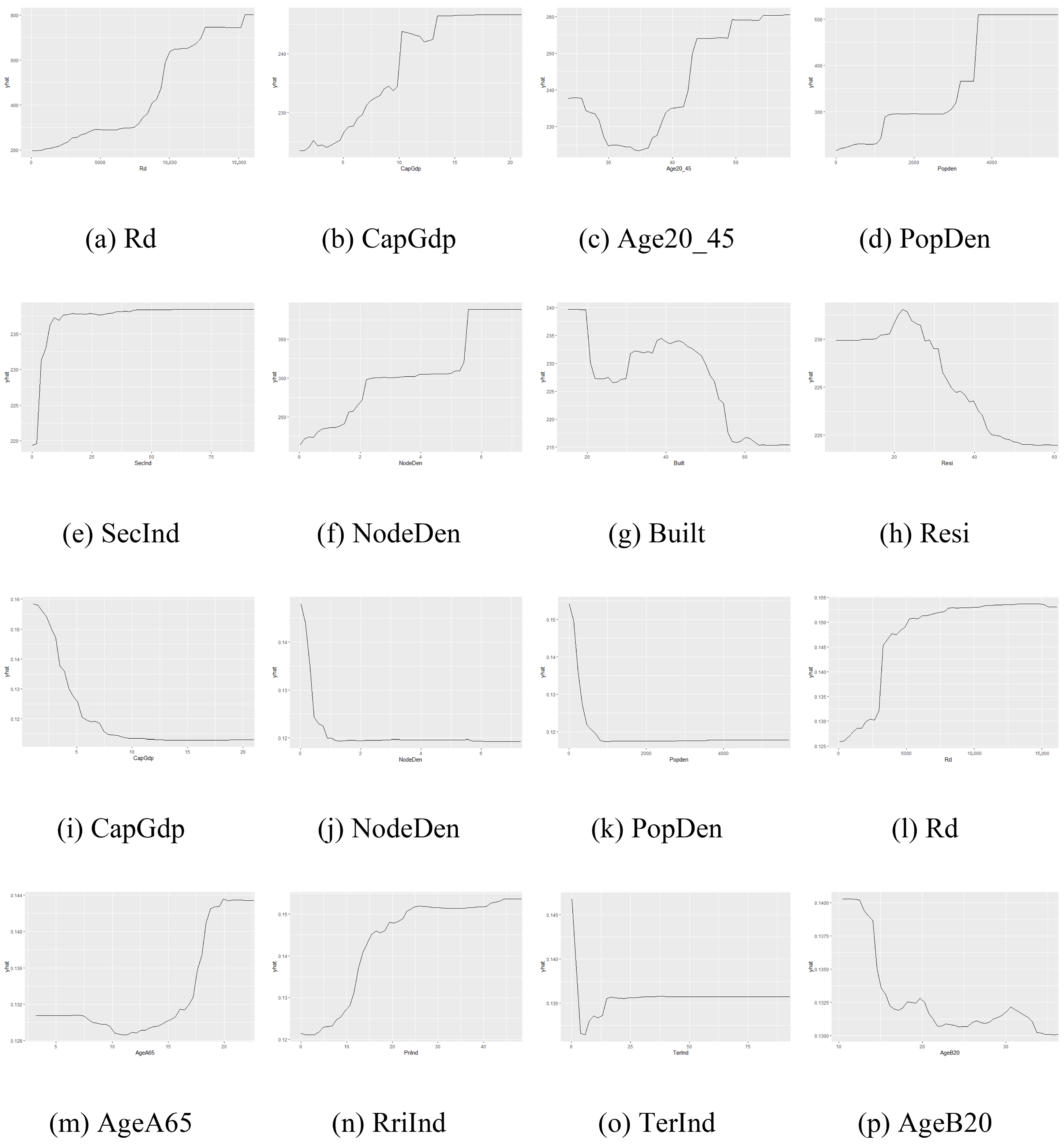
4.2.2. Explanatory Results

The contributions of explanatory variables for two dependent variables are also examined using the GWRF models. A higher incMSE value implies the variable is more important in the model. As shown in Figure 8, Rd, CapGdp, Age20_45, PopDen, SecInd, NodeDen, Built, and Resi make the highest contributions to CO2 emissions, while CapGdp, NodeDen, PopDen, Rd, AgeA65, PriInd, TerInd, and AgeB20 are the top eight important variables for the outcome, namely, CO2 emissions per GDP.
Partial dependence plots (PDPs) of the important explanatory variables are displayed using R (Version 4.2.3) package pdp [45]. The results regarding the correlation between emission and explanatory variables are consistent with the results from GWR (see Table 3). PDPs further describe Emi (Figure 9a–h) and GdpEmi (Figure 9i–p) as nonlinear functions and investigate whether the relationship between dependent variable and each contributing factor is linear, monotonic, curvilinear, or more complex [46]. The results show that most explanatory variables are not simply linearly associated with dependent variables. For example, Age20_45 is negatively associated (nonlinearly) with road traffic CO2 emissions when its value is lower than 35(%), but after this point, a positive nonlinear effect of Age20_45 on CO2 emissions is observed (Figure 9c). People aged 20 to 45 play an important role on traffic activity. Young people tend to generate lower carbon emissions due to their stronger environmental awareness. They are more likely to adopt low-carbon behaviors such as using public transportation, embracing shared mobility (e.g., bike-sharing). Nonetheless, as the proportion of people aged 20 to 45 continues to grow, the amount of traffic activity and carbon emissions will inevitably increase.
Approximately linear relationships are also found for several explanatory variables but only within some specific ranges. For example, there is an almost positive linear relationship between CapGdp and CO2 emissions at the range of 5–10, but outside of this range, the effect is fully nonlinear (Figure 9b). Similarly, there is an almost linear positive association between road area and CapEmi within the range of 0–2500, whereas the relationship is nonlinear outside this range (Figure 9i). Overall, the results indicate that most relationships between dependent variable and explanatory variables are nonlinear, which strengthens the advantage for using machine learning approaches to address the nonlinearity issue [29].

5. Conclusions

In this paper, conventional GWR, RF, and the proposed GWRF models are employed and compared to investigate the relationship between Chinese cities’ road traffic CO2 emissions and various contributing factors, including demographic, socioeconomic, road network, and built-environment characteristics. Two different measurements, namely, the total amount of emissions and emissions per GDP, are considered as the dependent variables of interest. Population density, GDP and per capita GDP, road area and per capita road area, and node density are found to have significant effects on both of the two dependent variables. By using spatial modeling approaches, we have found that various factors are associated with the road traffic CO2 emissions and emission efficiency across Chinese cities and regions. With such information, emission mitigation interventions could be tailored and implemented based on regional-specific situations and, hopefully, be more effective in reducing CO2 emissions. Specifically, developed cities should pay more attention to the optimization of road network structures, while undeveloped cities could make more efforts to develop public-transportation systems and intentionally control the increase in travel demand.
Regarding the models for road traffic CO2 emissions analysis, our results indicate that the GWRF model adopted in this study performs much better than the conventional GWR and RF models. Nonetheless, among GWRFs with different weight parameters, the local one (i.e., α = 1 ) was not the optimal. Therefore, an important procedure in practice is to find a proper weight and combine the local and global estimates to produce the final output. Additionally, our results for the partial dependence of the explanatory variables further imply that many contributing factors are nonlinearly associated with road traffic CO2 emissions. Such empirical evidence strengthens the practical necessity for applying flexible machine learning algorithms like GWRF due to their capability of handling spatial heterogeneity and complex nonlinearities.
It is important to recognize a few limitations. First, the cities without complete data are excluded from the analysis, which leads to the spatial discontinuity issue, thereby potentially adversely affecting the model performance. Second, due to the lack of detailed travel data in most cities, even though we have obtained comprehensive conclusions regarding the statistical relationships between road traffic CO2 emissions and contributing factors, the systematic mechanisms behind the effects of some factors remain under-explored, which deserve deeper investigation in the future using richer data.

Author Contributions

Conceptualization, D.W. and Y.Z.; methodology, D.W. and Y.Z.; software, D.W.; validation, H.J., D.W. and Y.Z.; formal analysis, D.W.; investigation, D.W.; resources, H.J.; data curation, D.W.; writing—original draft preparation, D.W.; writing—review and editing, H.J. and Y.Z.; visualization, D.W.; supervision, D.W. and Y.Z.; funding acquisition, H.J. All authors have read and agreed to the published version of the manuscript.

Funding

This research received no external funding.

Institutional Review Board Statement

Not applicable.

Informed Consent Statement

Not applicable.

Data Availability Statement

Data will be made available by the authors on request.

Conflicts of Interest

The authors declare no conflicts of interest.

References

  1. Statista. Transportation Emissions Worldwide. 2025. Available online: https://www.statista.com/topics/7476/transportation-emissions-worldwide (accessed on 13 April 2025).
  2. Wang, W.; Zhang, M.; Zhou, M. Using LMDI method to analyze transport sector CO2 emissions in China. Energy 2011, 36, 5909–5915. [Google Scholar] [CrossRef]
  3. Krause, J.; Small, M.J.; Haas, A.; Jaeger, C.C. An expert-based bayesian assessment of 2030 German new vehicle CO2 emissions and related costs. Transp. Policy 2016, 52, 197–208. [Google Scholar] [CrossRef]
  4. Oduro, S.; Ha, Q.; Duc, H. Vehicular emissions prediction with CART-BMARS hybrid models. Transp. Res. Part D Transp. Environ. 2016, 49, 188–202. [Google Scholar] [CrossRef]
  5. Grote, M.; Williams, I.; Preston, J.; Kemp, S. A practical model for predicting road traffic carbon dioxide emissions using Inductive Loop Detector data. Transp. Res. Part D Transp. Environ. 2018, 63, 809–825. [Google Scholar] [CrossRef]
  6. Fu, M.; Kelly, J.A.; Clinch, J.P. Estimating annual average daily traffic and transport emissions for a national road network: A bottom-up methodology for both nationally-aggregated and spatially-disaggregated results. J. Transp. Geogr. 2017, 58, 186–195. [Google Scholar] [CrossRef]
  7. Chuai, X.; Feng, J. High resolution carbon emissions simulation and spatial heterogeneity analysis based on big data in Nanjing City, China. Sci. Total Environ. 2019, 686, 828–837. [Google Scholar] [CrossRef]
  8. Li, Y.; Li, T.; Lu, S. Forecast of urban traffic carbon emission and analysis of influencing factors. Energy Effic. 2021, 14, 84. [Google Scholar] [CrossRef]
  9. Zhou, X.; Wang, H.; Huang, Z.; Bao, Y.; Zhou, G.; Liu, Y. Identifying spatiotemporal characteristics and driving factors for road traffic CO2 emissions. Sci. Total Environ. 2022, 834, 155270. [Google Scholar] [CrossRef]
  10. Wu, J.; Jia, P.; Feng, T.; Li, H.; Kuang, H. Spatiotemporal analysis of built environment restrained traffic carbon emissions and policy implications. Transp. Res. Part D Transp. Environ. 2023, 121, 103839. [Google Scholar] [CrossRef]
  11. Büchs, M.; Schnepf, S.V. Who emits most? Associations between socio-economic factors and UK households’ home energy, transport, indirect and total CO2 emissions. Ecol. Econ. 2013, 90, 114–123. [Google Scholar] [CrossRef]
  12. Wang, S.; Liu, X.; Zhou, C.; Hu, J.; Ou, J. Examining the impacts of socioeconomic factors, urban form, and transportation networks on CO2 emissions in China’s megacities. Appl. Energy 2017, 185, 189–200. [Google Scholar] [CrossRef]
  13. Eschmann, J.; Mueller, K.; Oesingmann, K.; Ennen, D. The economic implications of carbon neutrality ambitions in extra-European freight transport. Transp. Res. Part D Transp. Environ. 2025, 146, 104812. [Google Scholar] [CrossRef]
  14. Liu, X.; Wang, M.; Qiang, W.; Wu, K.; Wang, X. Urban form, shrinking cities, and residential carbon emissions: Evidence from Chinese city-regions. Appl. Energy 2020, 261, 114409. [Google Scholar] [CrossRef]
  15. Xie, R.; Fang, J.; Liu, C. The effects of transportation infrastructure on urban carbon emissions. Appl. Energy 2017, 196, 199–207. [Google Scholar] [CrossRef]
  16. Xu, C.; Zhao, J.; Liu, P. A geographically weighted regression approach to investigate the effects of traffic conditions and road characteristics on air pollutant emissions. J. Clean. Prod. 2019, 239, 118084. [Google Scholar] [CrossRef]
  17. Zhang, L.; Chen, H.; Li, S.; Liu, Y. How road network transformation may be associated with reduced carbon emissions: An exploratory analysis of 19 major Chinese cities. Sustain. Cities Soc. 2023, 95, 104575. [Google Scholar] [CrossRef]
  18. Song, L.; Cheng, H.; Wang, J.; Yu, S.; Du, Y. Geometric and operational optimization at reversible unconventional arterial intersection reducing traffic emissions. Transp. Res. Part D Transp. Environ. 2025, 141, 104656. [Google Scholar] [CrossRef]
  19. Shen, Y.S.; Lin, Y.C.; Cui, S.; Li, Y.; Zhai, X. Crucial factors of the built environment for mitigating carbon emissions. Sci. Total Environ. 2022, 806, 150864. [Google Scholar] [CrossRef]
  20. Wang, S.; Hu, M.; Li, J.; Liu, G.; Hu, W.; Qi, J.; Huang, J.; Liu, Z.; Wang, H.; Han, B. An interpretable spatially weighted machine learning approach for revealing spatial nonstationarity impacts of the built environment on air pollution. Build. Environ. 2025, 280, 113150. [Google Scholar] [CrossRef]
  21. Pallavidino, L.; Prandi, R.; Bertello, A.; Bracco, E.; Pavone, F. Compilation of a road transport emission inventory for the Province of Turin: Advantages and key factors of a bottom–up approach. Atmos. Pollut. Res. 2014, 5, 648–655. [Google Scholar] [CrossRef]
  22. Puliafito, S.E.; Allende, D.; Pinto, S.; Castesana, P. High resolution inventory of GHG emissions of the road transport sector in Argentina. Atmos. Environ. 2015, 101, 303–311. [Google Scholar] [CrossRef]
  23. Handy, S.L.; Boarnet, M.G.; Ewing, R.; Killingsworth, R.E. How the built environment affects physical activity. Am. J. Prev. Med. 2002, 23, 64–73. [Google Scholar] [CrossRef] [PubMed]
  24. Wang, L.; Xi, F.; Yin, Y.; Wang, J.; Bing, L. Industrial total factor CO2 emission performance assessment of Chinese heavy industrial province. Energy Effic. 2019, 13, 177–192. [Google Scholar] [CrossRef]
  25. Zhao, W.; Niu, D. Prediction of CO2 Emission in China’s Power Generation Industry with Gauss Optimized Cuckoo Search Algorithm and Wavelet Neural Network Based on STIRPAT model with Ridge Regression. Sustainability 2017, 9, 2377. [Google Scholar] [CrossRef]
  26. Sun, W.; Jin, H.; Wang, X. Predicting and Analyzing CO2 Emissions Based on an Improved Least Squares Support Vector Machine. Pol. J. Environ. Stud. 2019, 28, 4391–4401. [Google Scholar] [CrossRef]
  27. Khajavi, H.; Rastgoo, A. Predicting the carbon dioxide emission caused by road transport using a Random Forest (RF) model combined by Meta-Heuristic Algorithms. Sustain. Cities Soc. 2023, 93, 104503. [Google Scholar] [CrossRef]
  28. Georganos, S.; Grippa, T.; Niang Gadiaga, A.; Linard, C.; Lennert, M.; Vanhuysse, S.; Mboga, N.; Wolff, E.; Kalogirou, S. Geographical random forests: A spatial extension of the random forest algorithm to address spatial heterogeneity in remote sensing and population modelling. Geocarto Int. 2019, 36, 121–136. [Google Scholar] [CrossRef]
  29. Grekousis, G.; Feng, Z.; Marakakis, I.; Lu, Y.; Wang, R. Ranking the importance of demographic, socioeconomic, and underlying health factors on US COVID-19 deaths: A geographical random forest approach. Health Place 2022, 74, 102744. [Google Scholar] [CrossRef]
  30. Wu, D.; Zhang, Y.; Xiang, Q. Geographically weighted random forests for macro-level crash frequency prediction. Accid. Anal. Prev. 2024, 194, 107370. [Google Scholar] [CrossRef]
  31. Yazdian, H.; Salmani-Dehaghi, N.; Alijanian, M. A spatially promoted SVM model for GRACE downscaling: Using ground and satellite-based datasets. J. Hydrol. 2023, 626, 130214. [Google Scholar] [CrossRef]
  32. Zhang, Y.; Wang, X.; Zeng, P.; Chen, X. Centrality Characteristics of Road Network Patterns of Traffic Analysis Zones. Transp. Res. Rec. J. Transp. Res. Board 2011, 2256, 16–24. [Google Scholar] [CrossRef]
  33. Hadayeghi, A.; Shalaby, A.S.; Persaud, B.N. Development of planning level transportation safety tools using Geographically Weighted Poisson Regression. Accid. Anal. Prev. 2010, 42, 676–688. [Google Scholar] [CrossRef]
  34. Bao, J.; Liu, P.; Qin, X.; Zhou, H. Understanding the effects of trip patterns on spatially aggregated crashes with large-scale taxi GPS data. Accid. Anal. Prev. 2018, 120, 281–294. [Google Scholar] [CrossRef]
  35. Lu, B.; Harris, P.; Charlton, M.; Brunsdon, C.; Nakaya, T. GWmodel: Geographically-Weighted Models. 2013. Available online: https://doi.org/10.32614/cran.package.gwmodel (accessed on 13 April 2025).
  36. Breiman, L. Random Forests. Mach. Learn. 2001, 45, 5–32. [Google Scholar] [CrossRef]
  37. Janitza, S.; Hornung, R. On the overestimation of random forest’s out-of-bag error. PLoS ONE 2018, 13, e0201904. [Google Scholar] [CrossRef]
  38. Probst, P.; Wright, M.N.; Boulesteix, A. Hyperparameters and tuning strategies for random forest. WIREs Data Min. Knowl. Discov. 2019, 9, e1301. [Google Scholar] [CrossRef]
  39. Brunsdon, C.; Fotheringham, S.; Charlton, M. Geographically Weighted Regression. J. R. Stat. Soc. Ser. D 1998, 47, 431–443. [Google Scholar] [CrossRef]
  40. Kalogirou, S.; Georganos, S. SpatialML: Spatial Machine Learning. 2019. Available online: https://doi.org/10.32614/cran.package.spatialml (accessed on 13 April 2025).
  41. Marshall, W.E.; Garrick, N.W. Effect of Street Network Design on Walking and Biking. Transp. Res. Rec. J. Transp. Res. Board 2010, 2198, 103–115. [Google Scholar] [CrossRef]
  42. Zhou, Y.; Wang, H.; Qiu, H. Population aging reduces carbon emissions: Evidence from China’s latest three censuses. Appl. Energy 2023, 351, 121799. [Google Scholar] [CrossRef]
  43. Cervero, R.; Sarmiento, O.L.; Jacoby, E.; Gomez, L.F.; Neiman, A. Influences of Built Environments on Walking and Cycling: Lessons from Bogotá. Int. J. Sustain. Transp. 2009, 3, 203–226. [Google Scholar] [CrossRef]
  44. Gu, Y.; Liu, D.; Arvin, R.; Khattak, A.J.; Han, L.D. Predicting intersection crash frequency using connected vehicle data: A framework for geographical random forest. Accid. Anal. Prev. 2023, 179, 106880. [Google Scholar] [CrossRef] [PubMed]
  45. Greenwell, B.M. pdp: Partial Dependence Plots. 2016. Available online: https://cran.r-project.org/web/packages/pdp/index.html (accessed on 13 April 2025).
  46. Friedman, J.H. Greedy function approximation: A gradient boosting machine. Ann. Stat. 2001, 29, 1189–1232. [Google Scholar] [CrossRef]
Figure 1. Distribution of dependent variables: (a) CO2 emissions ( 10 4 tonne). (b) CO2 emissions per GDP (tonne/ 10 4 RMB).
Systems 13 00632 g001
Figure 2. Spatial distributions of the coefficients of population density: (a) Population density. (b) Coefficient in Model 1 (emission model). (c) Coefficient in Model 2 (efficiency model).
Systems 13 00632 g002
Figure 3. Spatial distributions of the coefficients of people aged above 65: (a) People aged above 65. (b) Coefficient in Model 1 (emission model). (c) Coefficient in Model 2 (efficiency model).
Systems 13 00632 g003
Figure 4. Spatial distributions of the coefficients of per capital GDP: (a) Per capital GDP. (b) Coefficient in Model 1 (emission model). (c) Coefficient in Model 2 (efficiency model).
Systems 13 00632 g004
Figure 5. Spatial distributions of the coefficients of road area: (a) Road area. (b) Coefficient in Model 1 (emission model). (c) Coefficient in Model 2 (efficiency model).
Systems 13 00632 g005
Figure 6. Spatial distributions of the coefficients of node density: (a) Node density. (b) Coefficient in Model 1 (emission model). (c) Coefficient in Model 2 (efficiency model).
Systems 13 00632 g006
Figure 7. MAPEs of models.
Systems 13 00632 g007
Figure 8. Distribution of dependent variables: (a) CO2 emissions ( 10 4 tonne). (b) CO2 emissions per GDP (tonne/ 10 4 RMB).
Systems 13 00632 g008
Figure 9. Partial dependence plots for the explanatory variables.
Systems 13 00632 g009
Table 1. Studies on contributing factors to road traffic carbon emissions.
CategoryIndependent VariablesReferences
Demographic and socioeconomic featuresPopulation, age structure, GDP, employment rate, industrialization level, private car ownershipBüchs and Schnepf (2013) [11];
Wang et al. (2017) [12];
Eschmann et al. (2025) [13]
Road network featuresRoad network density, road network topology structureLiu et al. (2020) [14];
Xie et al. (2017) [15];
Xu et al. (2019) [16];
Zhang et al. (2023) [17];
Song et al. (2025) [18]
Built environment featuresUrban form, land use patterns, urban transportation systemsShen et al. (2022) [19];
Zhou et al. (2022) [9];
Wang et al. (2025) [20]
Table 2. Descriptive statistics.
VariablesAbbreviationMinMaxMeanS.D.
Dependent variables
CO2 emissions ( 10 4 t)Emi112564226.73235.47
CO2 emissions per GDP (t/ 10 4 RMB)GdpEmi0.020.490.130.08
Socio-demographic
Population density (person/km2 )PopDen5.775698.55467.54548.41
Per capita GDP ( 10 4 RMB)CapGdp1.1215.143.09
Employment rate (%)Emp50.2799.7997.213.35
Primary industry (%)PriInd0.0448.3212.387.91
Secondary industry (%)SecInd15.1771.4546.579.56
Tertiary Industry (%)TerInd24.1779.6541.058.7
People aged below 20 (%)AgeB2010.4536.2622.695.51
People aged 20 to 45 (%)Age20_4523.6658.4732.545.05
People aged 45 to 65 (%)Age45_6519.5645.4430.654.53
People aged above 65 (%)AgeA653.222.6714.123.13
Road network
Paved roads ( 10 4 m2)Rd7016,1281968.912507.19
Node density (points/km2)NodeDen0.017.320.671.11
Built environment
Total urban area (km2)TotAr1201252,77716,691.6921,823.97
Built districts area (%)Built0.0345.071.833.9
Residential land area (%)Resi5.5160.8731.227.97
Urban green land area (%)Gre2.7151.4438.457.34
Public transportation vehicles per 10 4 populationPtVeh1.04225.59.6115
Table 3. Estimation results of the three models.
VariableModel 1 Emission ModelModel 2 Efficiency Model
Estimate Std.Error Estimate Std.Error
Intercept5.15 × 1029.17 × 1013.34 × 10−18.88 × 10⁻²
Popden9.23 × 10−22.82 × 10⁻²−1.01 × 10−41.76 × 10−5
Emp3.20 × 10−11.42 × 10⁻¹--
CapGdp7.908.99 × 10−1−1.64 × 10−22.58 × 10−3
Age20_457.761.13--
AgeA65−6.152.451.34 × 10−36.06 × 10⁻⁴
SecInd2.346.47 × 10−1--
TerInd--−1.78 × 10−38.34 × 10−4
Rd6.59 × 10−26.45 × 10−32.01 × 10−55.56 × 10⁻⁶
Nodeden1.54 × 1024.18 × 101−5.49 × 10−27.61 × 10−3
TotAr5.57 × 10−42.51 × 10⁻⁴--
Built−1.394.32 × 10−1--
Resi−1.114.21 × 10−1--
PtVeh--−1.05 × 10−25.00 × 10−3
Table 4. Estimation results of the models.
MetricGWRRFSpatial SVMGWRF
RMSE1.6521.3231.2581.146
MAPE0.1750.1340.1220.118
R20.6360.8320.8610.874
Disclaimer/Publisher’s Note: The statements, opinions and data contained in all publications are solely those of the individual author(s) and contributor(s) and not of MDPI and/or the editor(s). MDPI and/or the editor(s) disclaim responsibility for any injury to people or property resulting from any ideas, methods, instructions or products referred to in the content.

