Abstract
In the face of economic, social, and environmental pressures, the issue of sustainable development has garnered widespread attention in the Logistics Service Supply Chain (LSSC) with risk attitudes under Technical Output Uncertainty. In this regard, this paper first constructs an optimal emission reduction investment game model for an LSSC composed of Logistics Service Integrators (LSIs) and Logistics Service Providers (LSPs) against the backdrop of Technical Output Uncertainty. To this end, it quantifies the participants’ risk attitudes using a mean-variance model to analyze optimal emission reduction investment decisions for centralized and decentralized LSSC under different levels of risk tolerance. Subsequently, it designs a joint contract with altruistic preferences for sharing emission reduction costs in the LSSC. This contract analyzes the parameter constraints for achieving Pareto optimization within the supply chain. Finally, the study employs a case simulation to analyze the changes in expected revenues for centralized LSSC and joint contracts under different risk tolerance levels. The study reveals that (1) in a centralized LSSC, under risk-neutral attitudes, there exists a unique optimal emission reduction investment, which yields the highest expected return from emission reduction. However, under risk-averse attitudes, the expected return is always lower than the optimal expected return under risk neutrality. (2) In a decentralized LSSC, the emission reduction investment decisions of the Logistics Service Providers are similar to those in a centralized LSSC. (3) Under risk-neutral attitudes, the cost-sharing and altruistic preference-based joint contract can also coordinate the risk-averse LSSC under certain constraints, and by adjusting the cost-sharing and altruistic preference parameters, the expected returns can be reasonably allocated.
1. Introduction
In today’s rapidly evolving global economy, climate change has become a major issue for society, and the shift toward green and low-carbon development is inevitable. One of the main reasons for climate change is that global carbon emissions have considerably increased in recent decades, reaching 37.4 billion tons in 2023, a 1.1% increase from 2022, according to data from the International Energy Agency (IEA). In particular, emissions from fossil fuel power generation have a large share, contributing an additional 170 million tons and accounting for about 40% of last year’s total emissions increase. This high amount of emissions highlights the urgency of transitioning the entire industrial supply chain toward green and low-carbon solutions [1,2]. A major source of greenhouse gas emissions is the logistics sector, which is increasingly under scrutiny for its role in sustainable development. For example, the industry sector produces a substantial amount of carbon emissions in China due to its high energy-intensive nature, according to the “China Green Logistics Development Report (2023)”. Currently, carbon emissions from China’s logistic industries account for about 9% of the country’s total, with freight transportation and distribution activities responsible for approximately 85%. For this reason, logistic industries via green development can play a crucial role in achieving carbon neutrality across industrial supply chains due to the link between production and consumption. Transforming the logistic sectors into a green and low-carbon model is beneficial not only for their own sustainability but also for decarbonizing supply and value chains more broadly.
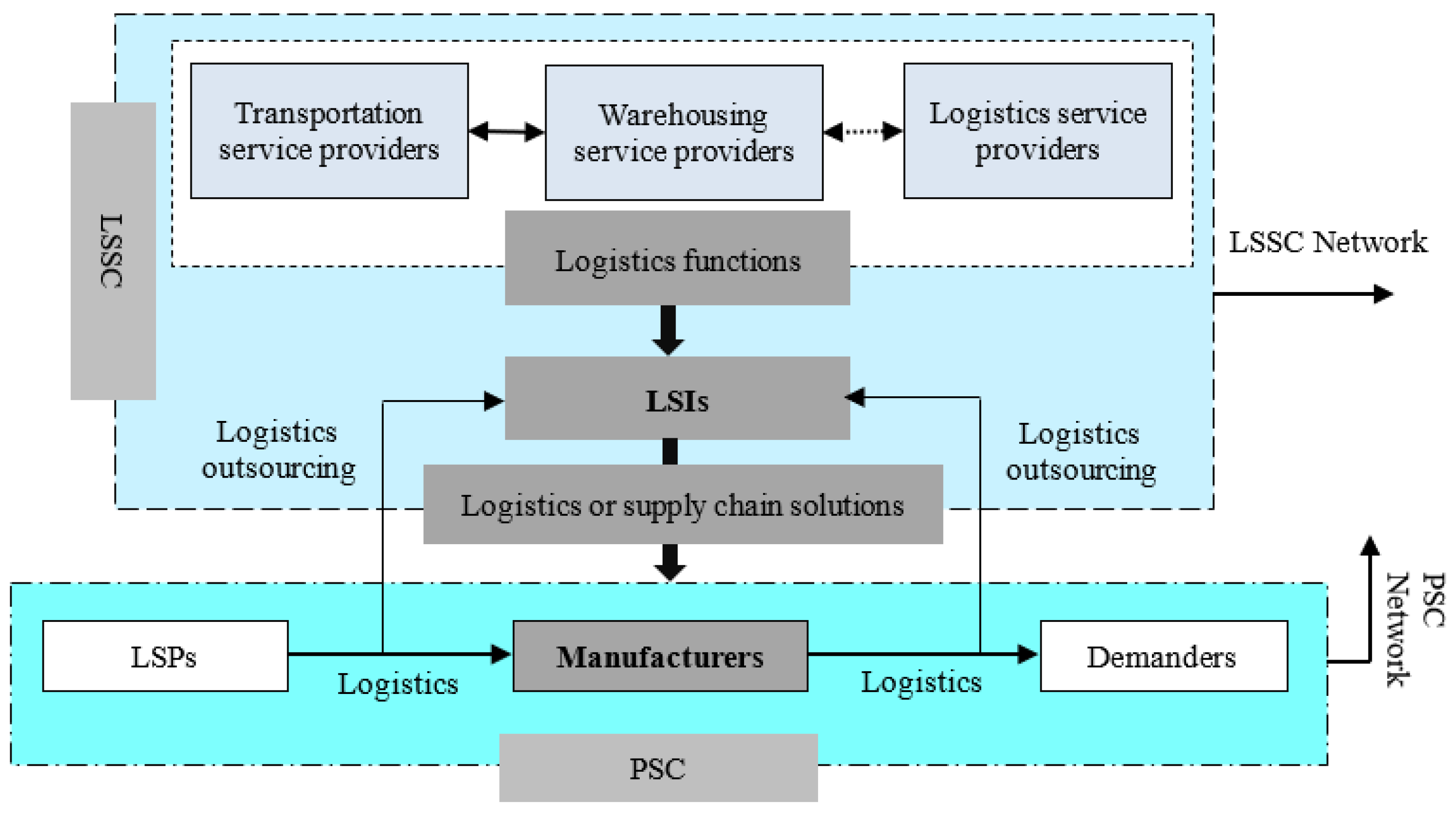
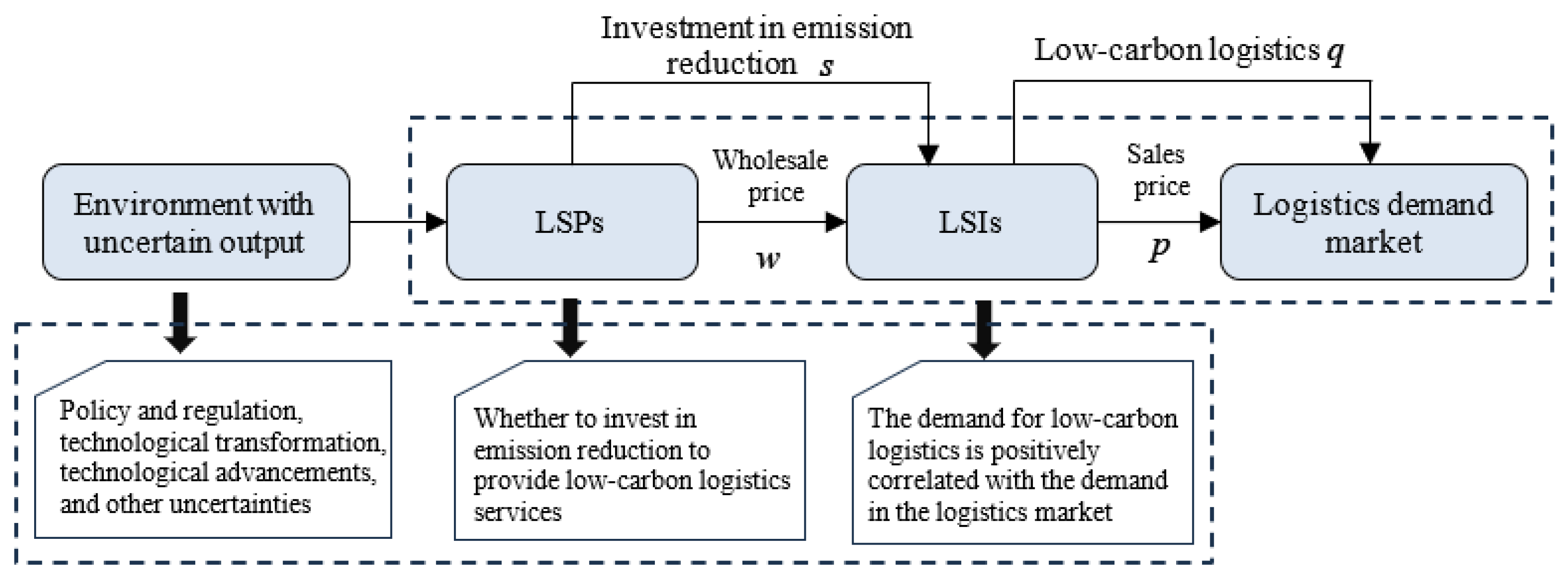
With the advancement of next-generation information technology, the modern logistics industry is shifting toward more efficient and intensive development. The scope and complexity of logistics service outsourcing are expanding, as various logistics organizations collaborate to meet demand and establish comprehensive service systems. These interactions create a multi-level supply and demand network, forming the LSSC. Figure 1 displays the LSSC in the context of logistics outsourcing within the product supply chain (PSC), which serves as a networked organization embedded in the PSC, delivering integrated logistics services to PSC enterprises. The LSSC, as a cross-enterprise organization, consists of LSIs and LSPs at various levels, representing a new management model. The LSSC shows a fundamental competition between system capabilities and supply chains. Building an efficient and collaborative logistics system is essential for the healthy development of the entire network.
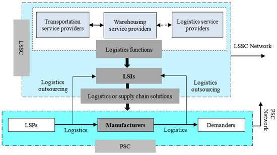
Figure 1.
Schematic diagram of the LSSC embedded in the PSC.
In recent years, under economic, social, and environmental pressures, LSSC enterprises have embraced green logistics by implementing various measures to reduce carbon emissions. These efforts reflect their commitment to promoting green and low-carbon practices throughout the supply chain [3]. However, the variety of low-carbon logistics technological innovations and their complex processes, which are affected by factors such as the natural environment, technological advancements, and trade tariffs, mean that emission reduction investments involve high costs and risks [4,5], leading to significant Technical Output Uncertainty in these investments. Particularly within some LSSCs, diversified LSIs play a dominant role, transferring the pressure of emission reduction investments upstream to LSPs, thereby reducing their own management costs. LSPs should set their planned production volumes under Technical Output Uncertainty, which guides their investments in low-carbon logistics capabilities. As a result, determining the optimal level of emission reduction investment becomes a key decision for LSPs. Like in the PSC, many smaller upstream providers with limited financial resources should also assess their risk tolerance when deciding on emission reduction investments in the face of Technical Output Uncertainty [6,7].
A similar scenario occurs in China’s Cainiao Smart Logistics Network Limited and its partnerships with upstream LSPs. In recent years, Cainiao Logistics has adhered to the strategy of digitization and globalization, deeply integrating the operation, scenarios, facilities, and information technology of the express logistics industry, and continuously promoting the construction of a smart logistics network. Driven by digital technology, Cainiao not only achieves emissions reduction through its own operations but also helps reduce emissions in the value chain. Cainiao released the “2024 Fiscal Year Environmental, Social and Governance Report”, which pointed out that Cainiao’s full-chain digital and intelligent logistics emission reduction solution covers all upstream and downstream links such as orders, warehousing, packaging, transportation, and recycling. By giving each package and commodity a digital ID, it further drives the collaborative carbon reduction in LSSC partners. The report shows that in the fiscal year 2024, Cainiao’s own operations and value chain achieved a reduction of 458,000 tons of emissions. Cainiao integrates online and offline operations through a digital platform business model, ordering low-carbon logistics directly from upstream partners, who then provide these services to customers. However, LSPs face Technical Output Uncertainty due to policy shifts and uncertainties in low-carbon technologies. These upstream enterprises should navigate dual risks from both technology and market forces when pursuing emission reduction efforts. As a result, when making emission reduction investment decisions, LSPs should carefully balance expected profits against potential risks to avoid significant losses.
The literature and corporate practices suggest that the issue of emission reduction in LSSCs, considering risk attitudes under Technical Output Uncertainty, is widespread. This paper considers the risk attitudes of LSPs under an environment of output uncertainty, providing decision-making support for their emission reduction investments. It also designs an effective joint incentive contract scheme based on cost-sharing and altruistic preferences for LSIs. This has important practical significance for addressing the emission reduction decision-making and contract coordination issues among participants in the LSSC. To this end, it focuses on the following key issues:
(1) In the face of Technical Output Uncertainty, how can centralized LSSCs and LSPs with varying risk tolerances and attitudes optimize their emission reduction investment decisions?
(2) In decentralized LSSCs, when LSPs exhibit varying levels of risk tolerance, how should LSIs determine appropriate joint contract parameters to ensure effective coordination within the LSSC?
(3) Based on different combinations of risk tolerance, how do variations in the range and degree of cost-sharing and altruistic preference joint contracts impact the Pareto optimization of emission reductions in the LSSC?
By addressing the aforementioned issues, this work contributes to the following key areas:
(1) Against the backdrop of Technical Output Uncertainty, this paper constructs a system model for emission reduction in the LSSC. It employs the mean-variance method to quantify decision-makers’ risk attitudes and explores optimal emission reduction investment decisions across various levels of risk tolerance within the LSSC.
(2) In decentralized LSSCs, this paper introduces a cost-sharing and altruistic preference joint contract to coordinate emission reduction investments and analyzes the conditions necessary for achieving Pareto optimization.
(3) Lastly, this research presents the joint contract parameters required for coordinating emission reductions in the LSSC and offers targeted management insights.
To address these issues, this study establishes the following structure. Section 2 reviews the relevant literature. Then, Section 3 outlines the fundamental issues related to Technical Output Uncertainty and constructs and solves the game model for emission reduction investment in the LSSC while considering risk attitudes. Subsequently, Section 4 analyzes the cost-sharing and altruistic preference joint contract, along with coordination strategies. Finally, numerical simulations are employed to explore the range and variations in Pareto optimization of the joint contract, validating the rationality and effectiveness of the proposed model.
2. Literature Review
As global environmental issues increasingly impact natural and human socio-economic systems, the pressure on the LSSC to reduce carbon emissions is becoming more urgent. LSPs and LSIs are also beginning to adopt various technological measures for a green transformation. Against this backdrop, this section outlines the relevant research areas: first, research on carbon emission reduction strategies for LSSC in a low-carbon environment; second, research on emission reduction inputs in supply chains considering risk attitudes under uncertain output conditions.
2.1. Emission Reduction Strategies in the LSSC Under a Low-Carbon Environment
Emission reduction investments in the LSSC under a low-carbon environment can be divided into two key aspects: technological measures and operational measures. Technological green investments focus on meeting emission reduction targets by enhancing energy efficiency or lowering emissions through innovations such as new engines, propulsion systems, and sustainable alternative fuels. Many scholars have examined technological green investments, analyzing their effectiveness and cost implications. For instance, Bai et al. [8] revealed that artificial intelligence was the most effective technology for achieving carbon emission reductions, followed by the Internet of Things, big data analytics, and cloud computing. These technologies often collaborated synergistically to achieve carbon reduction objectives. Additionally, Fang et al. [9] investigated the influence of various carbon policies and the integration of green technologies within a two-echelon supply chain, focusing on carbon emissions generated during the transportation, production, and storage phases. They also assessed the most effective investment in green technologies to reduce costs in the context of different carbon emission regulations. Furthermore, Jin et al. [10] explored cooperative emission reduction strategies between shipping companies and ports, based on mutual benefit. They introduced a joint mechanism characterized by “investment-first, reimbursement-later,” which contrasted with the previous “whoever pays taxes will reduce emissions” model, thereby encouraging proactive participation from key stakeholders, such as ports, in emission reduction efforts. Lastly, operational emission reduction measures in the LSSC focus on minimizing emissions from transport or warehousing by optimizing operational planning, such as whole-vehicle transportation and improved warehousing strategies [11,12]. Operational emission reduction measures are generally more flexible, requiring no large-scale investments. However, strategies like whole-vehicle operations, while effective in reducing emissions, may significantly impact the quality of logistics services.
In the context of the LSSC, research on low-carbon and green behaviors has mostly focused on analyzing green technology investment by individual enterprises, mainly from the perspectives of cost optimization and revenue management. However, limited studies have used theories, e.g., game theory, to explore how factors, like Technical Output Uncertainty and risk attitudes, affect decision-makers’ emission reduction investments. To address this gap, this paper incorporates risk attitudes into the LSSC under Technical Output Uncertainty, examining the participating entities’ emission reduction decisions.
2.2. Supply Chain Management Considering Risk Attitudes Under Technical Output Uncertainty
In supply chain risk research, scholars have increasingly focused on management issues related to decision-makers’ risk attitudes under Technical Output Uncertainty. They have employed various methods to analyze the impact of these risk attitudes, including prospect theory [13] and conditional value at risk (CVaR) [14,15]. However, the impact of decision-makers’ risk attitudes remains primarily concentrated in traditional supply chain research and is rarely explored in the context of LSSC. For example, Ma et al. [16] investigated the dynamic game of pricing and service strategies in a dual-channel supply chain, incorporating risk attitudes and free-riding behavior. They found that retailers with a higher tolerance for risk were more inclined to offer enhanced service levels. Fan et al. [17] explored the factors influencing the adoption of low-carbon supply chains by agricultural product consumers on major Chinese e-commerce platforms, employing an extended technology acceptance model. The study revealed that consumers’ perceived risk, perceived usefulness, and adoption attitudes significantly impacted their adoption behavior. Li et al. [18], by modeling uncertainty through risk attitudes (such as risk aversion and risk neutrality), constructed an electricity supply chain involving a power plant and an electricity retailer, each with distinct risk preferences. They developed optimal decisions for the supply chain under varying risk attitudes, highlighting the impact of these attitudes on decision-making.
Recently, a few scholars have begun to examine how risk attitudes affect LSSC management. For instance, Choi et al. [19] examined the effect of risk attitudes on freight rates in the competitive maritime logistics market, revealing the benefits of a risk-seeking attitude for firms under certain conditions. Choi et al. [20] further analyzed optimal dynamic strategies for resilient logistics under uncertainty, proposing conditions required for Pareto improvement in supply chains. Liu et al. [21] explored the influence of presale strategies and risk-averse behavior on the decisions and profits of logistics integrators in the context of demand updating. They found that when retailers adopted presale strategies with larger discounts, all potential customers would pre-order in the first period; otherwise, all potential customers would purchase in the second period. Zhang et al. [22] formulated a tripartite evolutionary game model to scrutinize the strategic interactions among government regulators, carriers, and contractors, providing insights into the collaborative supervision outcomes shaped by these stakeholder engagements.
In the LSSC, upstream LSPs face Technical Output Uncertainty and direct exposure to market demands, dealing with dual risks from both the supply and demand sides. Thus, understanding LSPs’ risk attitudes and their impact on investment decisions is of significant importance for the LSSC both theoretically and practically.
2.3. Literature Review Summary
The literature review highlights the notable progress of the research on low-carbon strategies in the LSSC under uncertain conditions, with the study of green strategies by logistics enterprises becoming a mainstream focus. However, certain deficiencies remain, as outlined below:
(1) Research on low-carbon strategies in logistics primarily focuses on individual enterprises, analyzing aspects such as route optimization, network planning, green upgrades, and site selection. However, emission reduction decisions depend significantly on participants’ networks in the LSSC, which can be totally disregarded in a merely single-enterprise perspective. Therefore, applying game theory and similar approaches to explore competitive and strategic interactions among entities presents a valuable avenue for addressing emission reduction and green transformation challenges in the logistics industry.
(2) Research that considers the impact of risk-averse attitudes on the LSSC remains quite limited. Existing studies on emission reduction strategies for logistics enterprises frequently assume that decision-makers exhibit risk-neutral and fully rational behavior. However, in real-world scenarios characterized by uncertainty, logistics enterprises often adopt a more cautious approach to mitigate the risks associated with green strategies. Therefore, analyzing decision-makers’ risk-averse behaviors in the context of Technical Output Uncertainty is of practical significance for optimizing supply chain strategies and ensuring an effective implementation of low-carbon initiatives.
Unlike previous studies, this paper begins with the context of Technical Output Uncertainty and employs a game model to analyze optimal emission reduction investment strategies in the LSSC, specifically considering a risk-averse inclination. It investigates how risk attitudes influence participant decisions and benefits through a mean-variance quantification model. Furthermore, the paper examines emission reduction decisions and contract coordination issues among participants, offering valuable insights. This approach not only complements existing theoretical research on the low-carbon development of the logistics industry but also provides new directions for future research, emphasizing the importance of understanding risk attitudes in the pursuit of sustainable logistics practices.
3. Model Construction
3.1. Problem Statement
In the context of low-carbon emission reduction, this paper constructs a two-tier LSSC system composed of an LSP and an LSI. The LSI orders low-carbon logistics from the upstream LSP according to the actual demand of the logistics market. The LSP, guided by service costs, technical standards, and other practical considerations, allocates resources and implements the production of low-carbon logistics orders. However, the LSP encounters various uncertainties that can significantly impact its operations, including national policies and regulations, the efficiency of technology conversion, and advancements in emission reduction technologies. These uncertainties introduce output risks, creating a gap between the expected output quantity and the actual input during the low-carbon service delivery process. Consequently, the LSP should address these challenges to optimize its resource allocation, ensuring the achievement of both operational targets and environmental commitments. Assumedly, the emission reduction input decided by the LSP as a follower is , at which point the actual low-carbon output is , where is a random low-carbon output variable, and follows a uniform distribution within [0, 1] [23,24]. represents the probability density function of , and denotes the cumulative distribution function of . Firstly, the LSI, as the leader in the LSSC’s emission reduction efforts, orders from the LSP based on the service demand for low-carbon logistics; then, the LSP, as a follower in the LSSC’s emission reduction, decides on the emission reduction investment . Due to the presence of output uncertainties and risks, the actual low-carbon output at this time is . The LSP incurs a unit emission reduction cost, , for each unit of low-carbon product invested and sells all low-carbon products to the LSI at the wholesale price . Additionally, the LSI sells low-carbon products at market price to the demanders. The LSSC’s emission reduction operations may raise two scenarios: First, if the supply of low-carbon logistics exceeds market demand, the LSP faces revenue losses due to redundant logistics capabilities; due to the nature of service products, excess service capacity has no value to the LSP, meaning the zero residual value of surplus low-carbon logistics capacity. Second, if the supply of low-carbon logistics is below market demand, the LSP faces a stockout penalty, , and the LSI faces a capability deficit penalty, . Figure 2 displays the specific system model.

Figure 2.
System model for emission reduction investment in the LSSC under Technical Output Uncertainty.
3.2. Centralized LSSC Emission Reduction Investment Model
This section constructs a centralized decision model for the LSSC, where it operates as a coordinated whole to optimize overall supply chain revenue. Based on the problem description, Equation (1) represents the revenue expression for the centralized LSSC:
Consequently, the standard deviation of revenue for the centralized LSSC is , where is expressed as:
Considering a risk-neutral centralized LSSC, the expected revenue expression is:
Since and , the expected revenue of the centralized LSSC is a strictly concave function with respect to . Therefore, under risk neutrality, the centralized LSSC has a unique optimal emission reduction investment, .
In a risk-averse case, the centralized LSSC can quantify the level of risk tolerance based on the mean-variance model. This paper employs the risk quantification model developed by Chiu et al. and Bai et al. [25,26], which uses the maximization of expected revenue, , as the objective function and the standard deviation of revenue, , as the risk constraint condition. The mean-variance model expression for the risk-averse centralized LSSC is:
where and represent the expected revenue and associated risk for a specific emission reduction investment within the centralized LSSC, respectively. reflects the volatility of emission reduction revenue within the centralized LSSC. The expression shows that as the price of low-carbon logistics and the penalty for shortages increase, the risk associated with emission reduction investments in the centralized LSSC continually rises. denotes the risk tolerance of the centralized LSSC for emission reduction, which has an inverse relationship with the degree of risk aversion, and the LSSC becomes risk-neutral when .
In practical business operations, the expected revenue from emission reduction investments in the centralized LSSC is . Assuming , solving equation yields two solutions: and . They represent two potential emission reduction investment decisions when the expected revenue of the centralized LSSC is zero. Considering the different risks associated with the two emission reduction investments and , the one with the lower standard deviation between and is chosen as the minimal risk tolerance when . Thus, the risk tolerance of the centralized LSSC must satisfy .
Theorem 1.
Under Technical Output Uncertainty, a unique emission reduction investment, , maximizes the revenue risk, , for the centralized LSSC.
Proof.
Expression (2) follows , and since , it is evident that . Further differentiation of yields . If , , and increases as increases; if , , and , meaning decreases as increases. Therefore, within interval , has a one-to-one relationship with and initially increases then decreases as increases. Concurrently, since the standard deviation , first increases and then decreases as increases, with a unique maximum at . The proof is complete. □
Based on Theorem 1, in a risk-averse environment, the revenue risk from emission reduction output in the centralized LSSC initially increases and then decreases with an increase in s. An explanation for this pattern is that when the emission reduction investment is at a lower level, the uncertainty in emission output causes the revenue volatility risk in the centralized LSSC to continually increase. As the emission reduction investment continues to increase to a certain level, the output of the LSSC can meet market demand, thereby decreasing the revenue volatility risk caused by Technical Output Uncertainty.
According to Theorem 1, when , the standard deviation of revenue for the centralized LSSC, , has a unique maximum value at . Let . When the risk tolerance of the centralized LSSC , the risk level is high and the LSSC has no risk constraints. In contrast, when , the risk level is low and the LSSC holds risk constraints. When the optimal risk-averse emission reduction investment coincides with the optimal risk-neutral emission reduction investment, the risk tolerance is calculated as .
Theorem 2.
Under risk neutrality and risk aversion, the emission reduction investments and in the centralized LSSC satisfy the following conditions: 1) when , ; and 2) when , .
Proof.
The optimal emission reduction investment for the centralized LSSC is under risk neutrality and under risk aversion. Comparing and shows that when , , and when , . The proof is complete. □
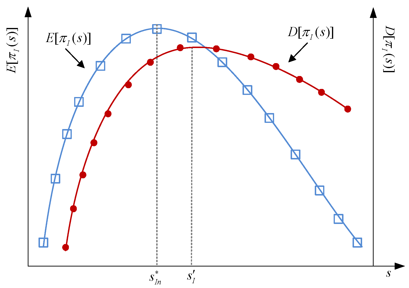
Figure 3 and Figure 4 illustrate this section, which depicts the trends in expected revenue and risk associated with changes in the emission reduction investment , as well as the positioning of different emission reduction investments and .

Figure 3.
Risk and expected revenue locations for the centralized LSSC (a).
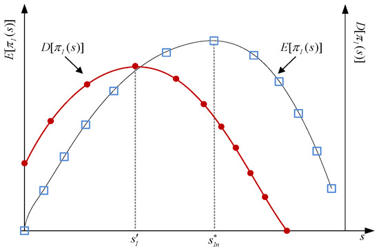
Figure 4.
Risk and expected revenue locations for the centralized LSSC (b).
According to Theorem 2, we compare the maximum emission reduction investment risks under risk aversion , risk neutrality , and zero expected revenue .
Proposition 1.
Under different risk attitudes, the emission reduction investment risks in the centralized LSSC satisfy .
Proof.
(1) Based on Theorem 2, when , . For , the emission reduction investment risk in the LSSC is a monotonically decreasing function of , thereby .
(2) Similarly, when , . For , the emission reduction investment risk in the LSSC is a monotonically increasing function of , thereby .
Hence, under different risk attitudes, the emission reduction investment risks in the centralized LSSC persistently satisfy . The proof is complete. □
According to Proposition 1, under Technical Output Uncertainty and when the LSSC’s emission reduction investment risk is at its maximum, the highest possible expected revenue is not higher than the emission reduction investment risk at the maximum expected revenue. This deviates from the classic input-output theory notion that “higher risk usually accompanies higher profit, while lower risk implies lower profit.” This indicates that under Technical Output Uncertainty, decision-makers in a risk-averse centralized LSSC cannot simply choose the optimal emission reduction investment based on general input theory, as the highest-risk emission reduction investment does not necessarily yield the highest expected revenue.
Considering the risk attitude of the centralized LSSC, in a risk-averse scenario, the decision-maker’s emission reduction investment is constrained by their level of risk tolerance, and the expected revenue may not achieve the optimal expected revenue . Concurrently, when the emission reduction investment risk tolerance of the centralized LSSC is (), let be the decision-maker’s optimal decision when . From earlier discussions, and from the expression for the standard deviation of revenue for the centralized LSSC, the emission reduction investment at risk tolerance is or . The expected revenues correspond to the emission reduction investments and are, respectively: , . Hence, the expected revenues from the two types of emission reduction investments in the centralized LSSC are not necessarily equal. At this point, equating , represents the risk when the two types of emission reduction investments achieve the same expected revenue, calculated as . Further analysis based on under different values can lead to Proposition 2.
Proposition 2.
Under Technical Output Uncertainty, the optimal emission reduction investment in the centralized LSSC satisfies the following conditions:
(1) When , ;
(2) When , , where:
(a) If , then ;
(b) If :
When , then ; when , then ; and when , then .
(c) If , then .
Proof.
(1) When , the quasi-concave nature of the revenue standard deviation in the centralized LSSC means that the optimal emission reduction investment is equal to that during risk neutrality, i.e., .
(2) When , , the following cases apply:
(a) If , the expected revenue of the LSSC necessarily satisfies ; thus, the optimal emission reduction investment is .
(b) If :
When , the expected revenue necessarily follows , thus .
When , the expected revenues are equal, , thus .
When , the expected revenue satisfies , thus .
(c) If , the expected revenue necessarily follows ; then the optimal emission reduction investment is .
The proof is complete. □
According to Proposition 2, under Technical Output Uncertainty, optimal emission reduction investment decision for the centralized LSSC depends on its own risk tolerance . When the LSSC has a high-risk tolerance (), the optimal emission reduction investment is unconstrained by risk, and its value is equal to the optimal investment under risk neutrality. In contrast, when it has a low-risk tolerance (), the optimal emission reduction investment is constrained by risk. In the latter case, the decision is required to be between and to yield the highest expected revenue. Given investment , the LSSC faces the risk of a capacity shortfall, primarily the risk of revenue loss and penalties due to insufficient capacity. Conversely, by choosing investment , the LSSC faces the risk of capacity redundancy, primarily the risk of revenue loss due to excess capacity. When the LSSC’s risk tolerance is , choosing between and is indifferent, implying an equal revenue loss from capacity shortfall and redundancy with and , respectively. Thus, unlike with a risk-neutral attitude, when adopting a risk-averse attitude, the centralized LSSC needs to assess its own risk tolerance. If its risk tolerance is high, its emission reduction investment decision is not constrained by risk. Conversely, if its risk tolerance is low, its decision must weigh the expected revenues of different investments to determine the optimal investment.
Proposition 3.
Under Technical Output Uncertainty, if the risk tolerance of the centralized LSSC ranges within , the relationship between the risk tolerance and the optimal emission reduction investment is as follows: and are monotonically increasing and decreasing functions of , respectively.
Proof.
From Proposition 2, if , the optimal emission reduction investment for the centralized LSSC is either or . Since both and are functions of , solving their first derivatives yields:
Hence, and . Accordingly, if , and satisfy the following relationship: and are monotonically increasing and decreasing functions of , respectively. The proof is complete. □
Based on Proposition 3, under Technical Output Uncertainty, if the centralized LSSC is constrained by risk , its optimal emission reduction investment, , is related to its risk tolerance, . When the optimal emission reduction investment is , the LSSC faces revenue losses due to capacity shortfall. Using Theorem 2, as the emission reduction investment increases, the revenue risk also continuously increases. Therefore, as increases and the LSSC has a higher risk tolerance, the supply chain will increase its emission reduction investment to reduce the risks associated with capacity shortfalls, thereby achieving higher expected revenues. When the optimal emission reduction investment is , the LSSC faces revenue losses due to capacity redundancy. Moreover, based on Theorem 2, as the emission reduction investment increases, the revenue risk continuously decreases. Thus, as increases and the LSSC possesses a higher risk tolerance, the supply chain will decrease its emission reduction investment to minimize the risks associated with capacity redundancy, thereby securing higher expected revenues.
3.3. Decentralized LSSC Emission Reduction Investment Game Model
This section analyzes the decentralized decision-making model of the LSSC, an important form of supply chain management that differs from the centralized LSSC in terms of organizational structure and operational mode. In a decentralized LSSC, the LSP and LSI operate independently, each aiming to maximize their individual interests, disregarding the impact on other members. Based on the assumptions described in the problem statement, Equation (4) constructs a game model under risk neutrality to provide an expected revenue expression for the LSP.
Similarly to the centralized LSSC, as and , the expected revenue for the LSP is a strictly concave function of . Under risk neutrality, the LSP holds a unique optimal emission reduction investment, . Additionally, to quantify the risk aversion of supply chain members, the standard deviation for the LSP’s revenue is , using the mean-variance model. Similarly, the expected revenue expression for the LSI is:
The standard deviation for the LSI, , and for , the decentralized LSSC’s emission reduction risk is equal to the sum of the emission reduction risks of the LSP and LSI, i.e., . This demonstrates that in the process of emission reduction investment within the LSSC, the risk caused by Technical Output Uncertainty does not change with the operational mode of the supply chain.
Considering that in the LSSC, the LSP is primarily responsible for emission reduction investments and bears the negative impacts caused by Technical Output Uncertainty, this article focuses on discussing the emission reduction investment model of the LSP under varying risk attitudes. It assumes a risk-neutral attitude for the LSI, implying that no risk constraint exists in decision-making.
Similarly to the decision-making model of the centralized LSSC, the mean-variance model expression for the LSP when considering risk aversion can be constructed as:
where maximizing the expected revenue of the LSP, , serves as the objective function, with the revenue standard deviation as the risk constraint, represents the risk tolerance of the decentralized LSP, where risk tolerance is inversely related to the degree of risk aversion, and denotes the risk tolerance when the LSP’s expected revenue is zero, with operational reality requiring , and as , the LSP is risk-neutral.
Given that under risk neutrality the only optimal emission reduction investment for the LSP is , at this point, its risk tolerance is , i.e., . Similarly to Theorem 1, under Technical Output Uncertainty, a unique emission reduction investment exists that maximizes the revenue risk for the decentralized LSP, . Comparing the decentralized LSP’s emission reduction investments and under different conditions: (1) when , and (2) when , .
Proposition 4.
Under different risk attitudes, the emission reduction investment risk for the decentralized LSP satisfies .
Proof.
(1) As per Theorem 2, when , because for , the emission reduction investment risk for the decentralized LSP is a monotonically decreasing function of , thus .
(2) Similarly, when , because for , the emission reduction investment risk for the decentralized LSP is a monotonically increasing function of , thus .
In summary, under different risk attitudes, the emission reduction investment risk for the decentralized LSP is . The proof is complete. □
Similarly to Proposition 1, according to Proposition 4, under Technical Output Uncertainty, the expected revenue at the maximum risk of emission reduction investment by the LSP does not exceed the risk at the highest expected revenue. Therefore, under the background of Technical Output Uncertainty, it cannot be assumed that the highest-risk emission reduction investments by a decentralized LSP will yield the highest expected revenue when adopting a risk aversion strategy.
When the risk tolerance of the decentralized LSP is (), let represent the LSP’s optimal decision within this range. Also, let ; the emission reduction investment for the LSP when its risk tolerance is can be either or . The expected revenues corresponding to these investment decisions are and . By setting , signifies the risk at which the LSP achieves the same expected revenue for both types of investment and is given by: . Further exploration into the optimal emission reduction investment, , establishes Proposition 5.
Proposition 5.
Under Technical Output Uncertainty, the optimal emission reduction investment, , for a decentralized LSP meets the following conditions:
(1) When , ;
(2) When , , where:
(a) If , then ;
(b) If , when , ; when , ; and when , .
(c) If , then .
Proof.
The proof of Proposition 5 follows a similar logic to that of Proposition 2. □
According to Proposition 5, under Technical Output Uncertainty, the optimal emission reduction investment decision for a decentralized LSP depends on its own risk tolerance . When the risk tolerance of the LSP is high, (), no risk constraint exists on the optimal investment, and its value equals that in the risk-neutral scenario. When the LSP’s risk tolerance is lower, (), the optimal investment faces risk constraints, balancing between and . If choosing results in a greater loss from insufficient capacity compared to the excess capacity loss from , the decision-maker opts for ; otherwise, is chosen. When the risk tolerance of the LSP is at , the outcomes of choosing or are financially equivalent, thus the decision-maker may select either without preference.
5. Numerical Simulation
This study investigates the optimal decision-making and coordination mechanisms for emission reduction investments in the LSSC under conditions of Technical Output Uncertainty, considering risk attitudes. To enhance the reliability and practical relevance of the research findings, it is based on firsthand data and operational practices gathered through field research and semi-structured interviews with typical LSSC enterprises in the Yangtze River Delta region of China. As one of the most economically dynamic, innovative, and integrated regions in China, with a highly developed logistics industry, the Yangtze River Delta hosts logistics companies (such as Cainiao Network, JD Logistics, SF Express, etc.) that have undertaken systematic zero-carbon engineering practices in areas such as green and low-carbon technology applications, promotion of new energy transportation tools, green warehousing construction, and optimization of energy structures. These efforts have led to the formation of a replicable case library. We deeply analyze the specific emission reduction measures, investment costs, and effectiveness data of these representative enterprises, and, by integrating insights from interviews regarding management challenges and risk considerations, refine key parameters (such as emission reduction cost coefficients, low-carbon technology applications, market uncertainty, and risk aversion levels). This ensures that the model parameters have a solid real-world foundation and industry representativeness, providing empirical support for theoretical analysis.
This study employs numerical examples to clearly compare the optimal emission reduction investment decisions under different risk attitudes within the LSSC, as well as the sensitivity of various contract coordination strategies to key parameters. It employs 2024b of MATLAB to conduct numerical simulations and examine the model’s feasibility and effectiveness. According to Proposition 2, under Technical Output Uncertainty, three scenarios exist for the optimal emission reduction investment, , in a centralized LSSC, varying with risk attitudes. To delineate how the optimal emission reduction benefits of the centralized LSSC vary with different risk attitudes, this paper sets the basic parameters for different constraint relationships of , , and , aligned with the actual emission reduction operations and cost–benefit characteristics of the case study companies. The specific parameter settings are as follows: if , then ; if , then ; if , then .
5.1. Expected Revenue in Centralized LSSCs Under Different Levels of Risk Tolerance
According to Proposition 2, the parameter ranges of , , and encompass the three scenarios of optimal emission reduction investment for a centralized LSSC, allowing for a comprehensive analysis of risk tolerance, , affecting the expected revenue of the LSSC. Regarding Figure 5, Figure 6, Figure 7 and Figure 8, under Technical Output Uncertainty, when , the risk tolerance exceeds the risk associated with the optimal emission reduction investment, , of the centralized LSSC. This implies that output risk poses no constraints on the LSSC, and the optimal emission reduction investment is the same for both risk-averse and risk-neutral conditions, (), in the centralized supply chain. However, when , output risk constrains the LSSC, leading to variations in the impact of different parameters on the optimal expected revenue of the centralized supply chain.

Figure 5.
Optimal expected revenue of a centralized LSSC’s emission reduction investment when .
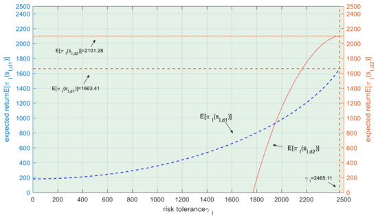
Figure 6.
Optimal expected revenue of a centralized LSSC’s emission reduction investment when .
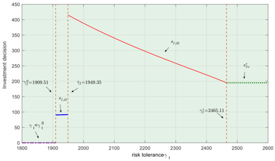
Figure 7.
Decision on emission reduction investment for a centralized LSSC under different risk tolerances.
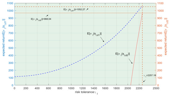
Figure 8.
Optimal expected revenue of a centralized LSSC’s emission reduction investment when .
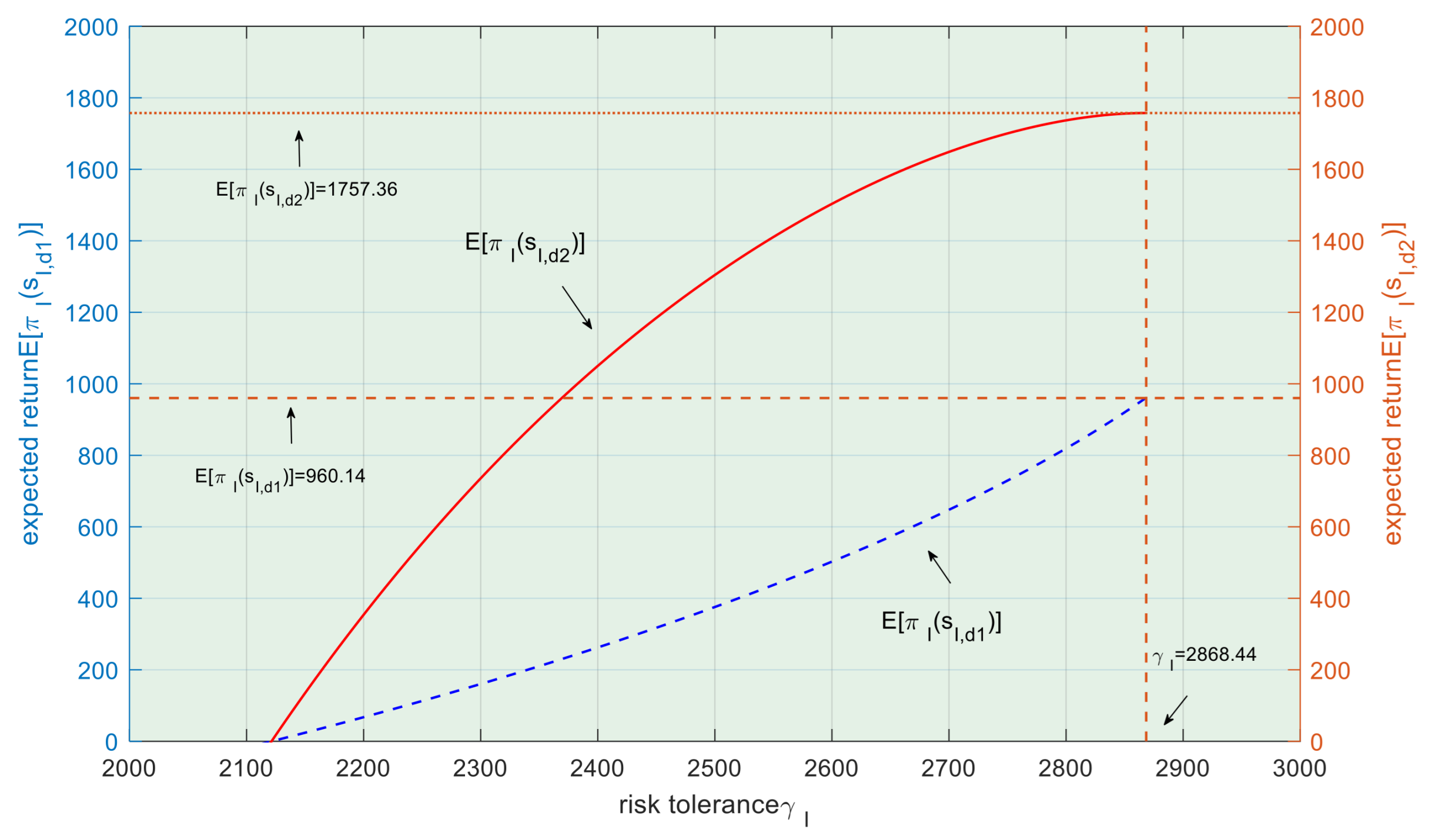
Figure 5 illustrates the scenario where , with the parameter combination for centralized LSSC emission reduction investment being . In this case, = 2296.09 and = 2121.32, satisfying . Under risk neutrality, the optimal emission reduction investment for the centralized LSSC is = 212.13, with the optimal expected revenue of = 1757.34, and the maximum emission reduction risk is = 2868.44. Based on Figure 5, when the centralized LSSC emission reduction risk is , the optimal emission reduction investment is not constrained by risk, and the optimal expected revenue equals the risk-neutral optimal expected revenue of 1757.34. Furthermore, given risk constraint , the optimal expected revenue from the emission reduction investment, , is greater than . Therefore, when , the optimal emission reduction investment is for the centralized LSSC.
First, Figure 6 illustrates the scenario where , with the parameter combination for centralized LSSC emission reduction investment being . At this point, = 1909.51, = 1949.35, and the maximum emission reduction risk is = 2465.11, satisfying . Under risk neutrality, the optimal emission reduction investment is = 194.94 for the centralized LSSC, and the optimal expected revenue is = 2101.28. According to Figure 6, when the centralized LSSC emission reduction risk is , the optimal emission reduction investment is not constrained by risk, and the optimal expected revenue equals the risk-neutral optimal expected revenue of 2465.11. When the risk tolerance of the centralized LSSC is = 1949.36, no difference exists between choosing or for the optimal emission reduction investment. In this case, the revenue loss caused by capacity shortage when choosing , , is equal to the revenue loss caused by capacity surplus when choosing , . When , the optimal expected revenue from emission reduction investment, , is greater than . When , the optimal expected revenue from emission reduction investment, , is greater than .
Second, Figure 7 shows the impact of risk tolerance on the optimal emission reduction investment for centralized LSSC when . If the risk tolerance of the centralized LSSC is , i.e., [1909.51, 1949.35), the optimal emission reduction investment is , which increases monotonically with the increase in risk tolerance . When the risk tolerance of the centralized LSSC is , i.e., = 1949.35, the choice between and yields the same optimal revenue. When the risk tolerance of the centralized LSSC is , i.e., (1949.35, 2465.11), the optimal emission reduction investment is , which decreases monotonically with the increase in risk tolerance . This analysis is consistent with the findings of Proposition 3.
Third, Figure 8 illustrates the scenario where , with the parameter combination for centralized LSSC emission reduction investment being . At this point, = 2257.18 and = 2473.86, satisfying . Under risk neutrality, the optimal emission reduction investment is = 137.44 for the centralized LSSC, with the optimal expected revenue of = 1052.27. With regard to Figure 8, when the centralized LSSC emission reduction risk , the optimal emission reduction investment is not constrained by risk, and the optimal expected revenue equals the risk-neutral optimal expected revenue of 1052.27. Additionally, when the risk constraint is , the optimal expected revenue from emission reduction investment, , is greater than . Therefore, when , the optimal emission reduction investment is for the centralized LSSC.
Therefore, this analysis validates the findings of Proposition 2.
5.2. Cost-Sharing Joint Contracts Under Altruistic Preference in LSSCs
Based on Proposition 5, when the level of risk tolerance falls within different ranges, the optimal emission reduction investment for centralized and decentralized LSSC differs, respectively, denoted as and . This section sets parameters as to analyze the coordination conditions under the cost-sharing joint contract with altruistic preference in LSSC. By configuring different combinations of and , the overall coordination is assessed under optimal emission reduction investments, thereby verifying the relevant analysis of Proposition 8.
Assuming a cost-sharing-altruistic preference joint contract with a shared emission reduction cost ratio of , the risk tolerance levels of the centralized LSSC are as follows: = 1909.50, = 1949.34, and = 2465.11, meaning . For the decentralized LSSC, the risk tolerance levels are = 1078.16, = 1516.57, and = 1479.06. Table 1 solves the altruistic preference coefficient required to achieve LSSC coordination, based on the risk constraint conditions, given different levels of risk tolerance, and .

Table 1.
Optimal emission reduction investment decisions under different levels of risk tolerance.
Table 1 indicates that, under the risk constraint conditions, given the emission reduction investment risks and for the centralized and decentralized LSSC’s provider, respectively, a unique altruistic preference coefficient exists that can achieve coordination of emission reduction investment. In addition, the expected revenue, , of the centralized LSSC is equal to the sum of the expected revenue of the LSI and the LSP in the decentralized LSSC. Similarly, the emission reduction investment risk in the centralized LSSC equals the total of the emission reduction investment risks of the LSI and the LSP in the decentralized LSSC.
Furthermore, we analyze the Pareto optimization effect of emission reduction investment under the cost-sharing-altruistic preference joint contract for the LSSC, using various combinations of risk tolerance as examples.
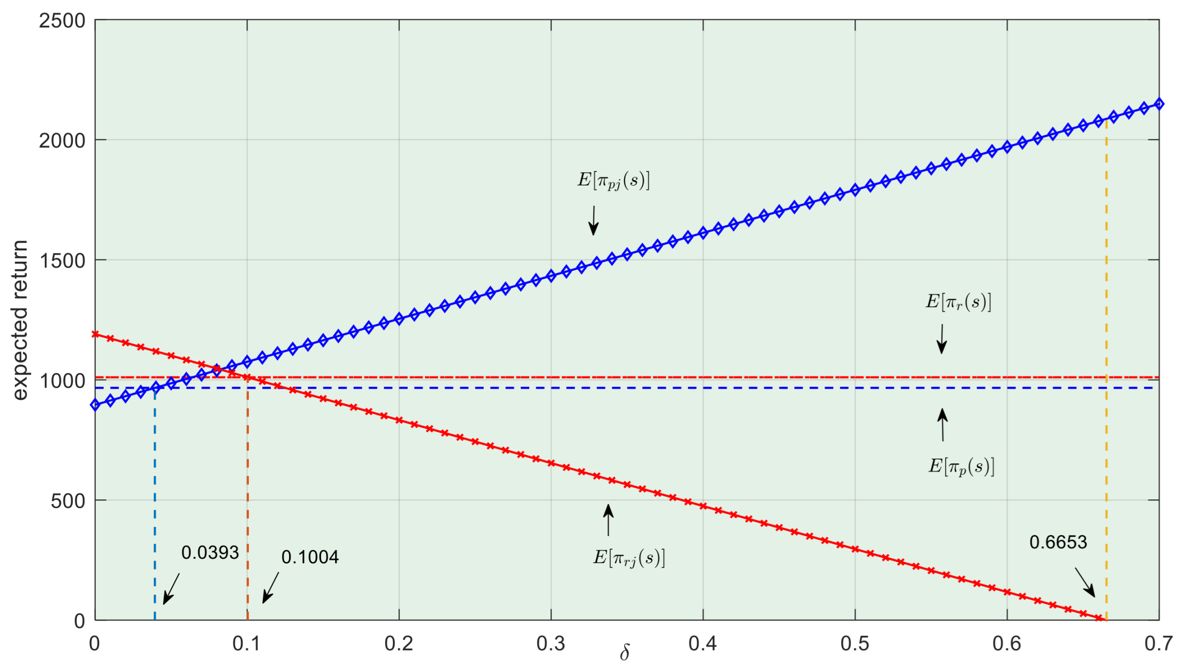
First, Figure 9 shows the changes in expected revenue under the cost-sharing-altruistic preference joint contract when = 2500 and = 1500, where both the centralized LSSC and the provider in the decentralized LSSC are not subject to risk constraints. After introducing the joint contract, the expected revenue of the supply chain varies with the shared emission reduction cost ratio . At this point, = 2465.11 and = 1479.06, satisfying and . The optimal emission reduction investment for the provider equals that of the centralized LSSC, = 178.93. When [0.0393, 0.1004], compared to the expected revenue under the decentralized LSSC contract, the expected revenue for both the LSP and LSI increases under the joint contract by 109.18. When > 0.6653, although the total expected revenue remains unchanged, the LSI’s expected revenue falls below 0 due to the high cost-sharing ratio, and the LSI will stop ordering low-carbon logistics.

Figure 9.
The effect of cost-sharing ratio δ on expected revenue when = 2500 and = 1500.
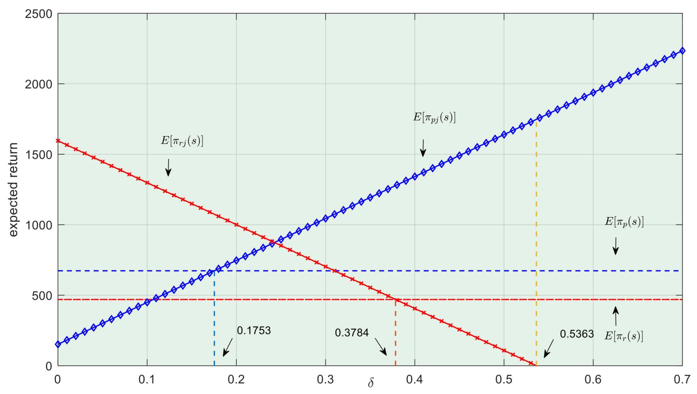
Second, Figure 10 shows the changes in expected revenue with the cost-sharing ratio when = 2200 and = 1300, where both the centralized and decentralized LSSC providers are subject to risk constraints. At this point, = 1949.34, = 2465.11, = 1300, and = 1479.06, satisfying and . Therefore, under the joint contract, the optimal emission reduction investment for the provider is = = 297.52, and for the decentralized LSSC provider, = 98.02. When [0.1753, 0.3784], the expected revenue for both LSP and LSI increases under the joint contract by 604.48. When > 0.5363, the expected revenue remains unchanged, but the LSI’s revenue drops below 0 due to the high cost-sharing ratio, causing the LSI to stop ordering low-carbon logistics and attempting LSSC’s emission reduction.
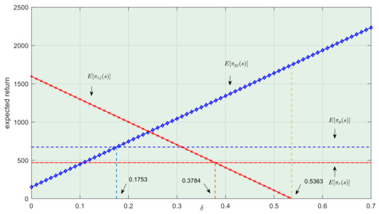
Figure 10.
The effect of the cost-sharing ratio δ on expected revenue when = 2200 and = 1300.
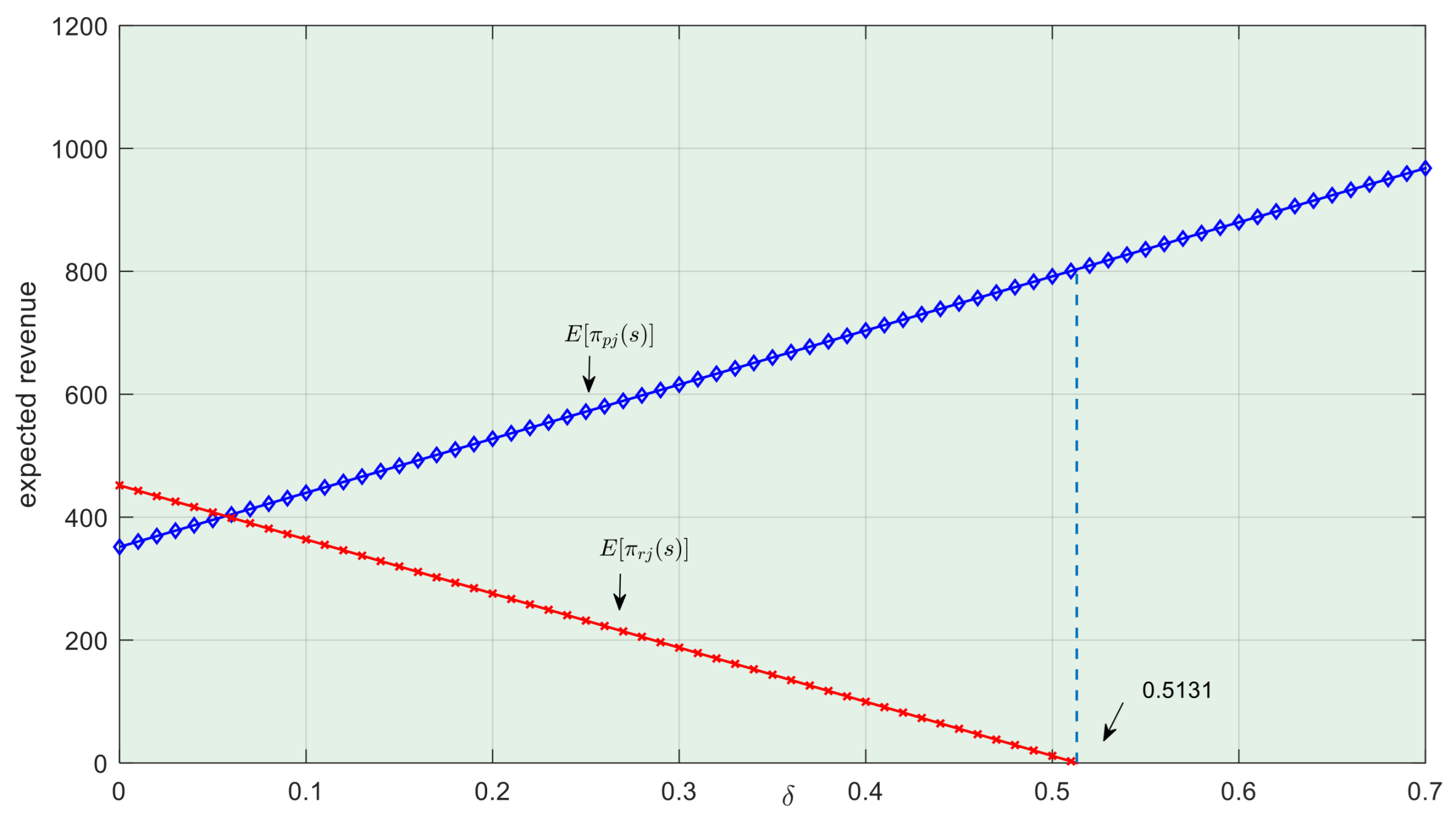
Lastly, Figure 11 shows the changes in expected revenue with the cost-sharing ratio δ when = 1800 and = 1000, where both the centralized and decentralized LSSC providers are below the minimum risk tolerance. After introducing the joint contract, the expected revenue of the supply chain changes with . At this point, = 1909.50 and = 1078.16, satisfying and . Under the joint contract, the optimal emission reduction investment for the provider is = 88.04, and when the decentralized LSSC provider’s risk tolerance is lower than , the provider offers no low-carbon logistics. When [0, 0.5131], the joint contract results in a positive expected revenue increase of 803.38 compared to 0 under the decentralized LSSC contract. When > 0.5131, the LSI’s revenue drops below 0 due to the high cost-sharing ratio, halting emission reduction efforts in the LSSC. This shows that with low-risk tolerance, setting an appropriate cost-sharing ratio, , and altruistic preference coefficient, , can enable both the LSP and LSI to continue emission reduction investments, achieving Pareto optimization in the LSSC under Technical Output Uncertainty.
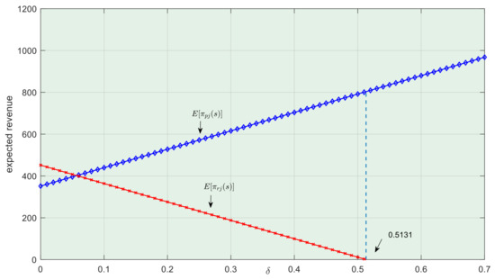
Figure 11.
The effect of cost-sharing ratio δ on expected revenue when = 1800 and = 1000.
In summary, the coordination of the cost-sharing-altruistic preference joint contract in the LSSC shows certain variations depending on the different risk tolerance scenarios. However, there is always a range of the emission reduction cost-sharing ratio, , for the LSI that can simultaneously increase the expected revenue for both LSP and LSI, achieving Pareto optimization of the overall revenue in the LSSC.
6. Conclusions and Implications
This paper investigates the optimal emission reduction investment decisions and coordination contracts for the LSSC, considering risk attitudes under different Technical Output Uncertainty conditions. Building on previous research, it integrates real-world issues faced by LSSC participants who are willing to forgo part of their revenue to mitigate the risks associated with emission reduction investments in the context of Technical Output Uncertainty. To this end, it constructs a decentralized LSSC system, consisting of one LSI and one LSP, with the risk attitudes of participants quantified through the mean-variance model. In this way, it explores optimal emission reduction investment decisions in a centralized LSSC under various combinations of risk tolerance. It also analyzes the coordination strategy for emission reduction investments in a decentralized LSSC when a cost-sharing-altruistic preference joint contract is introduced, along with the parameter constraints required to achieve LSSC coordination. The conclusions provide a scientific basis for emission reduction investment decisions and coordination contract design in the LSSC under the risks associated with Technical Output Uncertainty.
By exploring the mean-variance model to explore the emission reduction investment decisions in the LSSC under Technical Output Uncertainty, this paper draws the following main conclusions:
(1) Under risk neutrality, the centralized LSSC has a unique optimal emission reduction investment, allowing the supply chain to achieve the highest expected revenue from emission reduction. In contrast, under risk aversion, the expected revenue obtained by the centralized LSSC is consistently lower than the optimal expected revenue achieved under risk neutrality. As the emission reduction investment in the centralized LSSC increases, the associated risk follows a nonlinear pattern by initially rising and then declining. Consequently, at certain levels of risk tolerance, there are two potential emission reduction schemes. When the revenue loss resulting from capacity shortages is lower, the LSSC opts for a lower emission reduction investment as the optimal decision, maximizing expected revenue. However, when the revenue loss from capacity surplus is lower, the LSSC conversely chooses a higher emission reduction investment as the optimal decision but similarly results in the highest expected revenue.
(2) In the decentralized LSSC, the emission reduction investment decision made by the LSP mirrors that of the centralized LSSC. Furthermore, introducing a cost-sharing-altruistic preference joint contract can optimize the expected revenue from emission reduction in the decentralized LSSC within certain parameter conditions. The study demonstrates that, under risk neutrality, the implementation of the cost-sharing-altruistic preference contract can achieve Pareto optimization for the decentralized LSSC. Under risk aversion, both the centralized LSSC and the LSP may face risk constraints. However, under specific conditions, the cost-sharing-altruistic preference joint contract can facilitate coordination and Pareto optimization within the supply chain. Additionally, when considering different combinations of risk tolerance, the cost-sharing contract under altruism has various levels of effectiveness in the LSSC. Nonetheless, adjusting the cost-sharing and altruistic preference parameters can distribute the expected revenue of the decentralized LSSC in a reasonable manner among participants.
6.1. Managerial Insights
The conclusions demonstrate how optimal decisions for LSSCs change under Technical Output Uncertainty in various risk attitudes, which has theoretical significance and practical guidance value for the formulation of LSSC decisions, such as those of platforms like Cainiao Logistics.
(1) This paper offers practical recommendations for emission reduction investment decisions tailored to the varying risk attitudes of LSPs, specifically within the context of low-carbon development for logistics enterprises:
(a) Decision-making reference for risk-neutral managers: When managers adopt a risk-neutral attitude, the optimal emission reduction investment in a decentralized LSSC can yield the highest expected revenue. In this scenario, decision-makers primarily focus on maximizing expected revenue without overly emphasizing the risks associated with emission reduction.
(b) Decision balance for risk-averse managers: If managers are risk-averse, adopting more cautious emission reduction strategies leads to lower expected revenue compared to a risk-neutral approach. This occurs because risk-averse decision-makers prioritize mitigating the negative impacts of Technical Output Uncertainty, even by sacrificing some potential revenue.
(c) Key impacts of supply chain capacity status and strategy selection: Within an acceptable range of risk tolerance, two distinct investment strategies can achieve optimal expected revenue. Specifically, if the costs associated with insufficient capacity (e.g., shortages in low-carbon logistics supply) in the LSSC are low, firms may opt for a lower level of emission reduction investment to control costs while still maximizing expected revenue. Conversely, if the costs related to excess capacity (e.g., idle low-carbon transportation resources) are high, firms may choose a higher level of emission reduction investment to improve overall operational efficiency and maximize expected revenue.
Through this analytical framework, logistics enterprises can more effectively balance their emission reduction goals with expected revenue, thereby supporting sustainable low-carbon development in their business strategies.
(2) This paper also designs a cost-sharing-altruistic preference joint contract for LSSC emission reduction investment under different risk attitudes, promoting efficient cooperation among participants and achieving Pareto optimization in decentralized LSSCs. In the practice of low-carbon logistics, introducing a cost-sharing-altruistic preference joint contract mechanism can optimize expected revenue from emission reduction under certain parameter conditions. By sharing the emission reduction costs and emphasizing upstream social responsibility, all parties in the LSSC can achieve more effective cooperation for lowering carbon.
This study provides the following coordination strategies for logistics enterprise managers: (a) Under a risk-neutral scenario, a contract mechanism that combines cost-sharing and altruistic preference helps achieve Pareto optimization in decentralized LSSCs. In this way, it improves the overall revenue for all participants without harming the interests of any individual. (b) Under a risk-averse attitude, providers in a decentralized LSSC are constrained by their respective risk tolerances. However, under certain conditions, the cost-sharing-altruistic preference joint contract can still promote coordination in the decentralized LSSC and achieve Pareto optimization. Therefore, even when participants have differing risk attitudes, a well-designed contract can balance the interests of all segments in the LSSC.
This study also provides the following basis for policymakers to design incentive measures: The effectiveness of the joint contract in coordinating the LSSC may vary under different combinations of risk tolerance. However, adjusting the cost-sharing ratio and the level of altruistic preference can distribute the expected revenue between the LSI and the LSP in a more balanced way, supporting the sustainability of emission reduction efforts in the LSSC. This mechanism not only contributes to environmental protection but also strengthens collaboration among supply chain members, fostering the long-term development of logistics enterprises.
6.2. Future Research Directions
This study primarily focuses on optimal emission reduction investment decisions and contract optimization schemes for LSPs with different risk attitudes in a Technical Output Uncertainty environment. Consequently, potential future research directions include examining emission reduction decisions when LSIs exhibit varying risk attitudes and designing contract schemes for Pareto optimization in LSSCs. Additionally, further research could consider employing multi-agent simulation methods to construct dynamic game models that analyze the transmission mechanisms of emission reduction decisions under different risk attitude combinations, which is also an interesting research direction.
Author Contributions
Conceptualization, G.Z. and Z.Z.; methodology, G.Z.; software, Z.Z.; formal analysis, G.Z.; writing—original draft preparation, G.Z. and Z.Z.; writing—review and editing, G.Z. and Z.Z. All authors have read and agreed to the published version of the manuscript.
Funding
This work was supported by the Social Science Foundation of Shandong Province, grant number 24CJJJ25. 2023 Annual Project of Shenzhen “14th Five-Year” Education Science Plan (cgpy23022) and the Business Administration Discipline Construction Program of Shenzhen Polytechnic University (6022311006S).
Data Availability Statement
The original contributions presented in the study are included in the article; further inquiries can be directed to the corresponding author.
Conflicts of Interest
The authors declare no conflicts of interest.
References
- Fu, C.; Liu, Y.-Q.; Shan, M. Drivers of low-carbon practices in green supply chain management in construction industry: An empirical study in China. J. Clean. Prod. 2023, 428, 139497. [Google Scholar] [CrossRef]
- Xia, S.; Ling, Y.; De Main, L.; Lim, M.K.; Li, G.; Zhang, P.; Cao, M. Creating a low carbon economy through green supply chain management: Investigation of willingness-to-pay for green products from a consumer’s perspective. Int. J. Logist. Res. Appl. 2024, 27, 1154–1184. [Google Scholar] [CrossRef]
- Zhang, S.; Chen, N.; She, N.; Li, K. Location optimization of a competitive distribution center for urban cold chain logistics in terms of low-carbon emissions. Comput. Ind. Eng. 2021, 154, 107120. [Google Scholar] [CrossRef]
- Yin, H.; Zhao, J.; Xi, X.; Zhang, Y. Evolution of regional low-carbon innovation systems with sustainable development: An empirical study with big-data. J. Clean. Prod. 2019, 209, 1545–1563. [Google Scholar] [CrossRef]
- Golpîra, H.; Javanmardan, A. Robust optimization of sustainable closed-loop supply chain considering carbon emission schemes. Sustain. Prod. Consum. 2022, 30, 640–656. [Google Scholar] [CrossRef]
- Zou, H.; Qin, J.; Zheng, H. Equilibrium pricing mechanism of low-carbon supply chain considering carbon cap-and-trade policy. J. Clean. Prod. 2023, 407, 137107. [Google Scholar] [CrossRef]
- Ding, J. Role of risk aversion in operational decisions with remanufacturing under emissions price volatility. Comput. Ind. Eng. 2024, 189, 110013. [Google Scholar] [CrossRef]
- Bai, Y.; Xu, S. How does firm digitalisation drive management activities to achieve low-carbon development? Technol. Anal. Strateg. Manag. 2023, 1–16. [Google Scholar] [CrossRef]
- Fang, C.-C.; Hsu, C.-C. Enhancing efficiency in supply chain management: A synergistic approach to production, logistics, and green investments under different carbon emission policies. Int. J. Ind. Eng. Comput. 2025, 16, 159–176. [Google Scholar] [CrossRef]
- Jin, J.; Meng, L.; Wang, X.; He, J. Carbon emission reduction strategy in shipping industry: A joint mechanism. Adv. Eng. Inform. 2024, 62, 102728. [Google Scholar] [CrossRef]
- Jiang, J.; Zhang, D.; Meng, Q.; Liu, Y. Regional multimodal logistics network design considering demand uncertainty and CO2 emission reduction target: A system-optimization approach. J. Clean. Prod. 2020, 248, 119304. [Google Scholar] [CrossRef]
- Sikder, M.; Wang, C.; Yeboah, F.K.; Wood, J. Driving factors of CO2 emission reduction in the logistics industry: An assessment of the RCEP and SAARC economies. Environ. Dev. Sustain. 2024, 26, 2557–2587. [Google Scholar] [CrossRef]
- Wu, A.; Li, P.; Sun, L.; Su, C.; Wang, X. Evaluation Research on Resilience of Coal-to-Liquids Industrial Chain and Supply Chain. Systems 2024, 12, 395. [Google Scholar] [CrossRef]
- Zhang, M.; Shen, L.; Nan, J.; Wang, J.; Xia, Z.; Zhao, Y. Optimal strategies for supply chain with credit guarantee using CVaR. RAIRO-Oper. Res. 2024, 58, 2669–2682. [Google Scholar] [CrossRef]
- Jammernegg, W.; Kischka, P.; Silbermayr, L. Risk preferences, newsvendor orders and supply chain coordination using the Mean-CVaR model. Int. J. Prod. Econ. 2024, 270, 109171. [Google Scholar] [CrossRef]
- Ma, J.; Hong, Y. Dynamic game analysis on pricing and service strategy in a retailer-led supply chain with risk attitudes and free-ride effect. Kybernetes 2021, 51, 1199–1230. [Google Scholar] [CrossRef]
- Fan, X.; Zhang, Y.; Xue, J. Energy-Efficient Pathways in the Digital Revolution: Which Factors Influence Agricultural Product Consumers’ Adoption of Low-Carbon Supply Chains on E-Commerce Platforms? Systems 2024, 12, 563. [Google Scholar] [CrossRef]
- Li, D.; Xu, J.; Ibrahim, A.-W.; Liu, S. Facing renewable electricity production uncertainty: Decision-making and coordination of the electricity supply chain with different risk attitudes. J. Clean. Prod. 2025, 518, 145754. [Google Scholar] [CrossRef]
- Choi, T.-M.; Chung, S.-H.; Zhuo, X. Pricing with risk sensitive competing container shipping lines: Will risk seeking do more good than harm? Transp. Res. Part B Methodol. 2020, 133, 210–229. [Google Scholar] [CrossRef]
- Choi, T.-M. Facing market disruptions: Values of elastic logistics in service supply chains. Int. J. Prod. Res. 2021, 59, 286–300. [Google Scholar] [CrossRef]
- Liu, W.; Wei, S.; Shen, X.; Liang, Y. Coordination mechanism of logistic service supply chain: A perspective of presale sinking and risk aversion. Eur. J. Ind. Eng. 2023, 17, 310–341. [Google Scholar] [CrossRef]
- Zhang, M.; Shen, Q.; Zhao, Z.; Wang, S.; Huang, G.Q. Risk-Averse Behavior and Incentive Policies: A New Perspective on Spatial-Temporal Traceability Supervision in Construction Logistics Supply Chains. Comput. Ind. Eng. 2023, 192, 110256. [Google Scholar] [CrossRef]
- Fan, K.; Li, X.; Wang, L.; Wang, M. Two-stage supply chain contract coordination of solid biomass fuel involving multiple suppliers. Comput. Ind. Eng. 2019, 135, 1167–1174. [Google Scholar] [CrossRef]
- Shi, Y.; Wang, F. Revenue and risk sharing mechanism design in agriculture supply chains considering the participation of agricultural cooperatives. Systems 2023, 11, 423. [Google Scholar] [CrossRef]
- Chiu, C.-H.; Choi, T.-M. Supply chain risk analysis with mean-variance models: A technical review. Ann. Oper. Res. 2016, 240, 489–507. [Google Scholar] [CrossRef]
- Bai, Q.; Xu, J.; Chauhan, S.S. Effects of sustainability investment and risk aversion on a two-stage supply chain coordination under a carbon tax policy. Comput. Ind. Eng. 2020, 142, 106324. [Google Scholar] [CrossRef]


Disclaimer/Publisher’s Note: The statements, opinions and data contained in all publications are solely those of the individual author(s) and contributor(s) and not of MDPI and/or the editor(s). MDPI and/or the editor(s) disclaim responsibility for any injury to people or property resulting from any ideas, methods, instructions or products referred to in the content. |
© 2025 by the authors. Licensee MDPI, Basel, Switzerland. This article is an open access article distributed under the terms and conditions of the Creative Commons Attribution (CC BY) license (https://creativecommons.org/licenses/by/4.0/).