Distributed Trajectory Optimization for Connected and Automated Vehicle Platoons Considering Safe Inter-Vehicle Following Gaps

Abstract

Existing studies on platoon trajectory optimization of connected and automated vehicles face challenges in balancing computational efficiency, privacy, and safety. This study proposes a distributed optimization method that decomposes the platoon trajectory planning problem into independent individual vehicle tasks while ensuring safe inter-vehicle following gaps and maximizing travel efficiencyand ride comfort. The individual vehicle problems independently optimize their trajectory to improve computational efficiency, and only exchange dual variables related to safe following gaps to preserve privacy. Simulation experiments were conducted under single-platoon scenarios with different simulation horizons, as well as multi-platoon and platoon-merging scenarios, to analyze the control performance of the distributed method in contrast to the centralized method. Simulation results demonstrate that the mean computation time is reduced by 50% and the fuel consumption is decreased by 4% compared to the centralized method while effectively maintaining the safe inter-vehicle following gaps. The distributed method shows its scalability and adaptability for large-scale problems.

1. Introduction

Rapid urbanization has brought about significant challenges, including severe traffic congestion, environmental pollution, and traffic injuries. Connected and Automated Vehicles (CAVs), which integrate advanced communication and automation technologies, enable vehicles to exchange data with one another and with infrastructure for more coordinated operations. CAVs are seen as a promising solution to enhance traffic efficiency, improve safety, and alleviate congestion. Research on CAV trajectory planning and control makes substantial progress in recent years, yet it still faces notable challenges in computation scalability, coordination under uncertainty, and practical deployment constraints [1].

CAV trajectory optimization can determine the optimal driving trajectory to improve traffic capacity and safety. Research on trajectory optimization can be categorized according to the controlled vehicle numbers, i.e., an individual vehicle and a platoon of vehicles. The individual vehicle trajectory planning aims to optimize individual vehicle trajectories, thus enhancing driving efficiency and reducing fuel emissions. A multistage optimal control method that considers intersection queuing and traffic signal states is applied to update optimal speed trajectories in real time and reduce vehicle queuing at signalized intersections [2]. The branch-and-bound method combined with Kalman filtering is developed to improve trajectory planning accuracy [3]. An eco-driving strategy that improves safety is proposed to optimize the trajectory of individual vehicles in mixed traffic flows [4]. The improved Green Light Optimal Speed Advisory (GLOSA) systems are proposed using dynamic acceleration advice [5] or applying stochastic dynamic programming variants [6] for minimal delays and fuel consumption and enhanced computational efficiency. Reinforcement learning methods such as DDPG and SAC have been applied to optimize longitudinal trajectories under limited information, showing improved energy efficiency and safety over rule-based and human-driven baselines [7]. Although individual vehicle trajectory planning methods allow an individual vehicle to operate independently, they struggle to fully exploit the cooperative advantages of CAVs.

Platoon trajectory planning aims to optimize the overall traffic performance by planning vehicle trajectories considering platoon cooperation [8,9]. The Eco-Cooperative Adaptive Cruise Control (Eco-CACC) algorithm is designed to optimize the trajectories of vehicles passing through signalized intersections, which significantly reduces fuel consumption on single lanes [10]. Two-stage eco-driving systems improve fuel efficiency and operational performance but face computational burdens limiting application in dynamic traffic [11]. A two-layer control framework is established to optimize vehicle trajectories for platoon cooperative optimization but exhibits high computational complexity [12,13]. A bi-level framework is developed for cooperative group decision making, integrating behavior and trajectory modules based on complete traffic information, but it relies on centralized data aggregation and computation [14]. A speed-maximizing trajectory optimization model is proposed by executing the theoretical derivation based on queuing theory, and a discrete-time hybrid planning model is developed to boost system performance [15]. However, the method is computationally expensive in large-scale scenarios. In short, most platoon trajectory planning studies utilize centralized methods, but there is computational complexity in large-scale traffic scenarios and privacy leakage when processing various vehicle data.

Distributed methods are deemed promising to address the challenges of high computational complexity and privacy risks. A distributed trajectory optimization model demonstrates the high computational efficiency and minimal loss in system optimality on a single lane [16]. Distributed frameworks often optimize follower trajectories based on predicted or shared preceding behaviors, such as planned strategies or reference profiles, leading to coupling and communication burdens [17,18,19]. However, reliance on predicted trajectories complicates the problem and reduces the efficiency of the solution. A cooperative data-enabled predictive leading cruise control system divides the problem into subsystems, which require information exchange with preceding vehicles to suppress traffic fluctuations [20]. Furthermore, decentralized methods are also applied to optimize trajectories for fewer stop delays [21]. However, predicting preceding vehicle trajectories relies on car-following models and dynamic programming, limiting the accuracy of the solution. Distributed architectures reduce travel time and delays in roundabouts [22]. An optimization-free framework combining offline ecological trajectory generation with online trajectory selection has been shown to reduce computational complexity [23]. Despite these advances, current distributed methods often neglect safe following requirements and privacy protection. Safe following typically depends on predicting preceding vehicle trajectories, which is limited by prediction accuracy and increases privacy risks. Consequently, the effectiveness and applicability of existing distributed trajectory optimization methods remain uncertain in real-world traffic scenarios.

Despite notable progress in centralized and distributed trajectory optimization for connected and automated vehicles, significant challenges remain. Centralized methods provide globally optimal solutions but face limitations in scalability and raise privacy concerns due to extensive data sharing. Distributed methods improve scalability and privacy by decomposing the problem into local subproblems. However, they often rely on predicted trajectories to maintain safe following gaps. Such predictions can be inaccurate, potentially leading to instability. Moreover, many distributed frameworks inadequately address the safe following gap requirement, limiting their applicability in real-world traffic scenarios. These challenges highlight the need for distributed optimization methods that ensure both safety and computational efficiency.

To decompose the coupling effects arising from safe inter-vehicle following gaps, this study proposes a distributed trajectory optimization method to address the platoon trajectory planning problem for computational efficiency. A platoon trajectory controller is proposed to minimize travel time and maximize ride comfort by optimizing vehicle accelerations subject to admissible motions and safe following gaps. To separate the platoon trajectory control problem into multiple independent individual vehicle control subproblems, the constraint on safe following gaps is decomposed, and then dual decomposition is applied. Proximal minimization is used to update the dual variables, gradually improving the solution to the dual problem, bringing it closer to the optimal solution of the primal problem. Only dual variables are exchanged among CAVs, protecting the trajectory information privacy of individual vehicles. To validate the performance of the proposed distributed methods, a series of simulation experiments are designed considering vehicle numbers, simulation horizons, and platoon numbers in comparison to the centralized methods. The results demonstrate that the distributed method outperforms centralized methods on computation time and scalability while handling platoon size changes.

The organization of this paper is as follows. Section 2 formulates the problem and develops the vehicle trajectory optimization model. Section 3 proposes centralized and distributed solution methods after linearization. Section 4 and Section 5 analyze the simulation results of the solution methods. Finally, Section 6 concludes the paper.

2. Model Formulation

In this section, the optimal control problem of vehicle platoon trajectories is formulated, including decision variables, system dynamics, objective function, and controller constraints.

2.1. Problem Statement

This study aims to optimize the longitudinal trajectories of connected and automated vehicle (CAV) platoons to enhance driving efficiency and motion smoothness, while also improving computational efficiency and protecting individual vehicle privacy. A fully connected and automated environment is assumed, where lateral lane changes are excluded. Communication technologies, including vehicle-to-vehicle (V2V), vehicle-to-infrastructure (V2I), and infrastructure-to-vehicle (I2V), enable reliable information exchange across the platoon without considering communication delays or data losses.

To address the scalability limitations and privacy concerns of centralized methods in large-scale platoon optimization, a distributed optimization framework is adopted. The overall problem is decomposed into local subproblems for individual vehicles, which coordinate their control actions through limited information sharing. The control variable for each vehicle is its longitudinal acceleration, which is optimized under physical feasibility and safe inter-vehicle spacing constraints.

The optimization considers two main objectives: minimizing the absolute value of acceleration to improve motion smoothness, and maximizing the average speed to enhance overall driving efficiency. Safety is enforced through constraints on minimum following distances, acceleration limits, and speed bounds, which collectively ensure the feasibility and stability of platoon operations.

The proposed distributed method ensures coordination performance and safety compliance while maintaining scalability and privacy preservation, making it suitable for efficient control of large-scale vehicle platoons.

2.2. Control and State Variables

The control variables for the trajectory control problem are the accelerations of the vehicles over the simulation horizon. The simulation horizon length is defined by $K\in {\mathbb{Z}}^{+}$, where K represents the total number of discrete time steps and $\Delta t=1\mathrm{s}$ is the time step size. The time index is k ($\in \{1,2,\dots ,K\}$) over the simulation horizon. Let $i\in \{1,2,\dots ,N\}$ denote the index of a vehicle in the system, where N is the total number of vehicles. For vehicle trajectory planning, the control variable for vehicle i at time step k, denoted as $u_i\left(k\right)$, is the acceleration $a_i\left(k\right)$ expressed by

$$u_i\left(k\right)=a_i\left(k\right),k\in \{1,2,\dots ,K\}.$$

(1)

The state of the vehicle i at time step k is described by its longitudinal position $p_i\left(k\right)$ and speed $v_i\left(k\right)$. The state variable vector $x_i\left(k\right)$ is shown in

$$x_i\left(k\right)=\left[\begin{array}{c}{p}_i\left(k\right)\\ v_i\left(k\right)\end{array}\right],k\in \{1,2,\dots ,K\}.$$

(2)

2.3. System Dynamics

The system dynamics model for the optimal problem is presented. The following second-order equation describes the system dynamics for trajectory optimization:

$$x_i(k+1)=F{x}_i\left(k\right)+G{u}_i\left(k\right),$$

(3)

where

$$F=\left[\begin{array}{cc}1& \Delta t\\ 0& 1\end{array}\right],G=\left[\begin{array}{c}{\displaystyle \frac{1}{2}}\Delta t^2\\ \Delta t\end{array}\right].$$

(4)

2.4. Objective Function

Within the simulation horizon ($k\in \{1,2,\dots ,K\}$), the ride comfort and travel delay of all controlled vehicles are optimized by minimizing the absolute values of accelerations and maximizing vehicle speeds. The objective function is formulated as follows:

$$H=min\sum _{i=1}^N\sum _{k=1}^K\left[{\beta }_1\left|a_i\left(k\right)\right|-{\beta }_2{v}_i\left(k\right)\right],$$

(5)

where ${\beta }_1$ and ${\beta }_2$ are the cost weights associated with ride comfort and travel delay, respectively. The first term of the objective function aims to reduce fluctuations in acceleration, thus improving ride comfort, while the second term seeks to minimize travel delays by encouraging vehicles to accelerate.

2.5. Controller Constraints

The trajectory problem requires the control and state variables to satisfy certain constraints, including admissible accelerations, speed limits, and safe driving conditions. For trajectory optimization, the accelerations of all vehicles are bounded within an allowable range between the maximum acceleration, $a_{max}$, and the minimum acceleration (i.e., the negative of the maximum deceleration), $a_{min}$:

$$a_{min}\le a_i\left(k\right)\le a_{max}.$$

(6)

The speeds of all vehicles are restricted to be positive but not exceed the speed limit, $v_{max}$:

$$0\le v_i\left(k\right)\le v_{max}.$$

(7)

In terms of safe driving conditions, the following vehicles should maintain at least a minimal safe following inter-vehicle gap from the vehicles ahead. With $l_i$ representing the length of vehicle i, $t_{min}$ the minimum safe time gap between vehicles, and $s_0$ the minimum space gap under stationary conditions, the safety requirements can then be expressed as

$$p_{i-1}\left(k\right)-p_i\left(k\right)-v_i\left(k\right)t_{min}-s_0-l_i\ge 0,i\ge 2.$$

(8)

3. Solution Method

To solve the CAV trajectory control problem, a centralized method and a distributed method are presented after linearizing the trajectory planning model.

3.1. Linearization

To simplify the objective function in Equation (5), two auxiliary non-negative variables $q_i\left(k\right)$ and $r_i\left(k\right)$ are introduced. These variables are defined as follows:

$$q_i\left(k\right)={\displaystyle \frac{|a_i\left(k\right)|+a_i\left(k\right)}{2}},q_i\left(k\right)\ge 0,$$

(9)

$$r_i\left(k\right)={\displaystyle \frac{|a_i\left(k\right)|-a_i\left(k\right)}{2}},r_i\left(k\right)\ge 0.$$

(10)

As a result, the accelerations and the ride comfort cost term can be represented by

$$a_i\left(k\right)=q_i\left(k\right)-r_i\left(k\right),q_i\left(k\right)\ge 0,r_i\left(k\right)\ge 0,$$

(11)

$$|a_i\left(k\right)|=q_i\left(k\right)+r_i\left(k\right),q_i\left(k\right)\ge 0,r_i\left(k\right)\ge 0.$$

(12)

The auxiliary variables $q_i\left(k\right)$ and $r_i\left(k\right)$ can be treated as extra control variables within the controller, subject to the linear equality constraints of Equations (11) and (12). Replacing the ride comfort cost term in the objective function using Equation (12), the control problem is reformulated as follows:

$$H=min\sum _{i=1}^N\sum _{k=1}^K\left[{\beta }_1\left(q_i\left(k\right)+r_i\left(k\right)\right)-{\beta }_2{v}_i\left(k\right)\right],$$

(13)

subject to the constraints of Equations (6)–(8).

3.2. Centralized Method

The centralized method is widely used in CAV platoon trajectory optimization, ensuring global optimization for the entire platoon. In this study, the centralized optimization is conducted with an Intel(R) Core(TM) i5-12500 processor and 8 GB of RAM. The optimization model of Equation (13) is solved via MATLAB R2023b with the linprog solver using the dual-simplex method. The constraint tolerance of ${10}^{-4}$ and the optimality tolerance of ${10}^{-7}$ ensure an efficient solution to the optimal vehicle trajectories. The convergence tolerance used in the solver was maintained at ${10}^{-4}$, which corresponds to the default setting and has been verified to yield reliable and stable solutions for this problem.

3.3. Distributed Method

This distributed method [24] is applied using dual decomposition and proximal minimization to solve optimization problems in multi-agent systems with coupling constraints. The optimization problem involves multiple agents, each with its own local objective function and constraints, and a coupling constraint that models resource sharing. The coupling constraint is expressed as the non-positivity of the sum of certain functions, each depending on the decision variables of an individual agent. By reformulating the problem as a dual optimization problem, the global objective is decomposed into local subproblems that agents can solve independently. The algorithm combines primal and dual updates to coordinate the agents’ decisions. It guarantees convergence to optimal solutions under convexity and connectivity conditions. In this study, this distributed algorithm is adapted to address the platoon trajectory optimization problem by decomposing it into individual vehicle trajectory optimization tasks.

3.3.1. Dual Problem

According to [25], the trajectory optimization problem of Equation (13) is formulated as

$$min\sum _{i=1}^N{c}_i^{\top }{u}_i,$$

(14)

subject to

$$\sum _{i=1}^N{A}_i{u}_i\le b,u_i\in U_i,$$

(15)

where $c_i$ in Equation (14) represents the coefficients of the local cost function for the i-th vehicle, and $c_i^{\top }{u}_i$ denotes the objective function for vehicle i, given in Equation (5). The total objective function of the platoon is the sum of the individual objectives. Equation (15) defines the coupling constraint as the sum of the safety gaps between adjacent vehicles. The matrix $A_i$ relates the decision variables $u_i$ to the safety gap between vehicle i and its neighbors. The vector b specifies the ideal safe inter-vehicle following gaps across the entire platoon. $U_i$ is the domain of the decision variable, related to constraints Equations (6), (11), and (12).

The dual problem of Equation (14) is given by

$$\underset{\lambda \ge 0}{max}-{\lambda }^{\top }b+\sum _{i=1}^N\underset{u_i\in U_i}{min}\left(c_i^{\top }{u}_i+{\lambda }^{\top }{A}_i{u}_i\right),$$

(16)

where $\lambda \ge 0$ is the global dual variable linked to the global coupling constraints in Equation (15).

The separable inner problem is expressed as

$$u_i\left(\lambda \right)\in arg\underset{u_i\in U_i}{min}\left(c_i^{\top }{u}_i+{\lambda }_i^{\top }{A}_i{u}_i\right).$$

(17)

This structure allows the inner problems to be solved independently for each vehicle, enabling parallel computation. With more vehicles, the system benefits from greater computational power, ensuring robust computational performance.

3.3.2. Distributed Optimization

Dual decomposition is applied to decompose the global problem into individual trajectory optimization tasks for each vehicle, allowing each vehicle to solve its own dual problem independently. The safety gap constraint of Equation (8) is a coupling constraint among vehicles (namely agents), aiming to maintain the safe distance between adjacent vehicles. To decompose the coupling effect of the safety gap constraint, each vehicle optimizes its trajectory by solving its dual problem of Equation (17). The local controller minimizes delays and maximizes comfort subject to local constraints on admissible acceleration and speed as well as the safety gap, as defined by Equations (6)–(8). By solving the individual dual problems independently, the overall platoon trajectory is optimized.

To ensure that the solution approximates the optimal solution of the primal problem, proximal minimization is applied. The subgradient is used as the proximal term to penalize deviations between the actual inter-vehicle distance and the desired safety gap. During each iteration, the dual variables are updated based on this penalty, refining the vehicle trajectories until the inter-vehicle distances converge to the desired safety gap. Regarding convexity and connectivity, The objective functions are convex, ensuring a unique optimal solution. Connectivity facilitates effective communication between vehicles, allowing for the simultaneous optimization of trajectories. These conditions guarantee that the optimization process converges to the globally optimal platoon trajectory. The process of the distributed method is detailed below.

Step 1: Initialization. Initialize the primal decision variables $u_i^{\left(0\right)}\in U_i$ for all vehicles $i=1,\dots ,N$ and set the dual variable ${\lambda }^{\left(0\right)}=0$. Define the step size ${\alpha }_{\tau }$ and the convergence tolerance $ϵ>0$, and set $\lambda \ge 0$.

Step 2: Local Optimization. At each iteration $\tau$, each vehicle i solves its local trajectory optimization problem independently:

$$u_i(\tau +1)=arg\underset{u_i\in U_i}{min}\left(c_i^{\top }{u}_i+\lambda {\left(\tau \right)}^{\top }{A}_i{u}_i\right).$$

(18)

Step 3: Dual-Variable Update. After all agents compute their local solutions, $\lambda$ is updated globally using the subgradient method. The update is performed as

$$\lambda {(\tau +1)}^{\top }={\left[\lambda {\left(\tau \right)}^{\top }+\alpha \left(\tau \right)\left(\sum _{i=1}^N{A}_i{u}_i(\tau +1)-b\right)\right]}_{+},$$

(19)

where ${[·]}_{+}$ denotes projection onto the non-negative orthant. The term ${\sum }_{i=1}^N{A}_i{u}_i(\tau +1)-b$ serves as a subgradient of the dual function (as shown in Equation (17)) with respect to $\lambda$. By iteratively adjusting $\lambda$ along this subgradient direction, the algorithm ensures that the dual variables converge to their optimal values under appropriate step size $\alpha$. $\alpha$ is computed using ${\displaystyle \frac{{10}^{-5}}{\tau +1}}$ [26].

Step 4: Convergence Check. Evaluate the stopping criteria:

$$\parallel \lambda (\tau +1)-\lambda \left(\tau \right)\parallel <ϵ.$$

(20)

If the condition is met, the iterative process terminates. Otherwise, the algorithm returns to Step 2 to continue the iteration. Algorithm 1 details the distributed optimization method.

To leverage computational efficiency and solution accuracy, the initial dual-variable update gradient $\alpha$ is configured as 0.0001 to determine the initial iteration direction and speed. The dual-variable update coefficient $\rho$ is chosen as 0.99 to regulate the magnitude of dual-variable updates. The convergence tolerance $ϵ$ is $5\times {10}^{-7}$.

Algorithm 1: Distributed optimization method

Initialization: 1: $\tau =0$ 2: $u_i^{\left(0\right)}\in U_i,\forall i=1,\dots ,N$ 3: ${\lambda }^{\left(0\right)}=0,\lambda \ge 0$ Iteration: 4: while $\parallel {\lambda }^{(\tau +1)}-{\lambda }^{\left(\tau \right)}\parallel > ϵ$ do: 5:     Initialize $u_i^{(\tau +1)}$ for $i=1,\dots ,N$ 6:     for each $i=1,\dots ,N$ do: 7:       Calculate Equation (18) 8:       Calculate Equation (19) 9:     end for 10:     $\tau \leftarrow \tau +1$ 11: end while Return:${\left\{u_i^{(\tau +1)}\right\}}_{i=1}^N,{\lambda }^{(\tau +1)}$

4. Simulation and Results

In this section, multiple simulation experiments that were conducted to validate the performance of the distributed method, considering different numbers of vehicle platoons, controlled vehicles, and the simulation horizons, are presented. Multiple scenarios were designed to analyze the performance of the distributed method compared with the centralized method.

4.1. Experiment Design

In designing the simulation experiments, several key factors significantly impact vehicle platoon control performance. The size of the platoon influences the stability of the traffic flow and the capacity of the system, thus affecting the control complexity and computational demands [27,28]. The length of the simulation horizon plays a critical role in the performance of automated vehicles, affecting safety, comfort, and efficiency, across varying optimal horizons [29]. Multi-platoon scenarios introduce additional challenges related to coordination, communication, and scalability [30]. Furthermore, platoon-merging maneuvers require precise coordination and significantly affect control results [31]. Based on these factors, four simulation scenarios are designed to systematically evaluate the proposed distributed and centralized methods.

Four scenarios were designed to evaluate control performance, as shown in

Table 1. Experimental settings.

Scenario	Platoon Setting	Vehicle Number	Simulation Horizon (s)	Initial Platoon Leader Position (m)	Objective
1	Single	2, 4, …, 24	130	0	Test the impact of different single-platoon vehicle numbers
2	Single	20	110, 120, …, 200	0	Test the impact of different simulation horizons
3	Multiple	4, 8, …, 40	130	400	Test the impact of different total vehicle numbers in multi-platoons
4	Multiple	32	130	400	Validate the control performance in platoon merging

. Scenarios 1 and 2 focus on a single platoon, while scenarios 3 and 4 involve multiple platoons. Scenario 1 analyzes the impact of varying vehicle numbers within a single platoon with a simulation horizon of 130 s. The number of vehicles increases from 2 to 24 in increments of 2 to test different platoon sizes. Scenario 2 examines the impact of the simulation duration in a single platoon of 20 vehicles. The simulation duration increases from 110 to 200 s in 10 s intervals. Scenario 3 investigates the influence of total vehicle numbers in two platoons with an inter-platoon distance of 400 m and a simulation duration of 130 s. Each platoon starts with 2 vehicles, increasing in increments of 2 vehicles, such that the total number of vehicles is increased from 4 to 40 vehicles. Scenario 4 validates the control performance in platoon merging with a simulation duration of 130 s. Each platoon is configured with 16 vehicles, so a total of 32 vehicles are considered.

The parameter settings are described in

Table 2. Parameter values.

Notation	Description	Value	Unit
$\Delta t$	Time step	1	s
K	Simulation horizon in scenarios 1 to 4	130, 110 to 200, 130, 130	s
N	Total number of vehicles in scenarios 1 to 4	2 to 24, 20, 4 to 40, 32	veh
${\beta }_1$	Ride comfort weight coefficient	10	s
${\beta }_2$	Delay weight coefficient	1	-
$a_{min}$	Minimum acceleration	−5	m/${\mathrm{s}}^2$
$a_{max}$	Maximum acceleration	2	m/${\mathrm{s}}^2$
$v_{max}$	Maximum speed	15	m/s
$l_i$	Length of vehicle i	3	m
$t_{min}$	Minimum safe time gap	2	s
$s_0$	Minimum space gap at standstill	2	m
–	Initial position	0, 400	m
–	Initial inter-vehicle gap	21	m
–	Initial speed	8	m/s
–	Inter-platoon gap in scenarios 3 and 4	400, 245	m

. Similar settings can be implemented without difficulty. The simulation time step is set to 1 s, which balances computational efficiency and the ability to capture key vehicle dynamics and control responses. Given the total feedback and actuation delays are less than 1 s, this step size can appropriately represent system behavior with acceptable accuracy. The vehicle length is set to 3 m as a representative value for a compact car to maintain model simplicity. The minimum safe time gap is set to 2 s to ensure a conservative and safe following distance between vehicles in the model.

To analyze the operational and computational performance of the distributed and centralized methods, performance metrics are selected, including the objective function value Equation (13), fuel consumption, and computation time. Fuel consumption ($\mathrm{mL}·{\mathrm{m}}^{-1}·{\mathrm{veh}}^{-1}$) is calculated using the instantaneous fuel consumption model [32] and the travel distance, where the coefficients $b_0$, $b_1$, $b_2$, $b_3$, $c_0$, $c_1$, and $c_2$ are $0.1569$, $2.450\times {10}^{-2}$, $-7.415\times {10}^{-4}$, $5.975\times {10}^{-5}$, $0.07224$, $9.681\times {10}^{-2}$, and $1.075\times {10}^{-3}$, respectively.

$$f(a,v)=\left\{\begin{array}{cc}{b}_0+b_{1}v+b_2{v}^2+b_3{v}^3+a\left(c_0+c_{1}v+c_2{v}^2\right),\hfill & a>0,\hfill \\ b_0+b_{1}v+b_2{v}^2+b_3{v}^3,\hfill & a\le 0.\hfill \end{array}\right.$$

(21)

4.2. Simulation Results of Distributed and Centralized Methods

In this section, the optimal trajectory performance of the centralized and distributed methods in four scenarios is presented as shown in Figure 1, Figure 2, Figure 3, Figure 4, Figure 5, Figure 6, Figure 7, Figure 8, Figure 9, Figure 10 and Figure 11. It is clear that both methods satisfy the controller constraint and fulfill the control objectives. The detailed analysis of four scenarios is discussed below.

4.2.1. Single-Platoon Scenario 1

In scenario 1, simulation results for 24 vehicles are presented to analyze the performance of the distributed and centralized methods, including acceleration, longitudinal trajectories, and the space gap between adjacent vehicles; see Figure 1, Figure 2, Figure 3 and Figure 4.

As shown in Figure 1, the vehicles using the distributed and centralized methods first accelerate and then maintain the maximum speed. The last vehicle using the distributed method reaches a maximum speed of 15 m/s at 50 s and a final position of 1129 m at 130 s. Since the distributed method relies on local information exchange, each vehicle only needs to perceive the speed and position of the preceding vehicle. Therefore, the accelerating time for each vehicle is 4 s, and occurs sequentially with each vehicle waiting for the preceding vehicle to complete its speed adjustment, as shown in Figure 2a. However, the last vehicle using the centralized method begins acceleration at 38 s, takes 35 s to reach approximately 15 m/s at 73 s, and then maintains this speed. Since all vehicles receive the command simultaneously but must match the preceding vehicle’s speed, acceleration delays accumulate sequentially, as shown in Figure 2b.

The inter-vehicle gap in Figure 3a under the distributed method increases to 35 m from 0 to 50 s. The gap and speed changes show high consistency due to local information exchange, and safe inter-vehicle distances depend not only on basic safety parameters but also directly on the speed of the following vehicle, as shown in Equation (8). However, as shown in Figure 3b, the inter-vehicle gap using the centralized method converges at 35 m at 75 s, showing delayed adjustments in vehicle space gaps.

Vehicle accelerations show similar features. As shown in Figure 4a, acceleration using the distributed method rises sharply from 0 to 2 ${\mathrm{m}/\mathrm{s}}^2$, then drops abruptly to 0. This reflects the distributed optimization strategy that prioritizes reaching the target acceleration quickly through local information exchange, although it comes at the cost of acceleration smoothness. In contrast, as shown in Figure 4b, the acceleration obtained by the centralized method increases from 0 to 2 ${\mathrm{m}/\mathrm{s}}^2$ and then decreases more gradually. Preceding vehicles maintain smooth acceleration due to global planning, whereas following vehicles experience more fluctuations as they make multiple adjustments to keep the safe gap and maintain ride comfort.

4.2.2. Single-Platoon Scenario 2 with Different Simulation Horizon

In scenario 2, the simulation results for 20 vehicles with a simulation duration of 180 s are presented to analyze the performance of the distributed and centralized methods. To conserve space, only acceleration and speed are presented, while the similar performance of space gaps and longitudinal positions as in scenario 1 is omitted.

Vehicles first accelerate and then maintain maximum speed (see Figure 5 and Figure 6). It can be seen that, with a longer simulation horizon, vehicles in scenario 2 begin to accelerate earlier, and the space gap increases earlier than in scenario 1. As shown in Figure 5a, the last vehicle (the 20th) begins acceleration at 38 s and reaches maximum speed at 42 s. Under the distributed method, each vehicle optimizes its trajectory to reach maximum speed as quickly as possible, so the acceleration phase remains nearly constant and unaffected by the extended simulation horizon. In contrast, the centralized method predicts vehicle state changes ahead and makes global decisions. The last vehicle (the 20th) using the centralized method accelerates at 31 s and takes 32 s to reach 15 m/s at 63 s; see Figure 5b. In Figure 6b, more vehicles in scenario 2 exhibit larger variations to maintain platoon coordination, while the distributed method is hardly affected by the extended simulation horizon.

4.2.3. Multi-Platoon Scenario 3

In scenario 3, the simulation results of position trajectories, speed, and space gap for 40 vehicles in a multi-platoon scenario with a simulation duration of 130 s are presented; see Figure 7, Figure 8 and Figure 9. The space gap is plotted on a logarithmic scale in Figure 9.

The trajectories generated by the distributed and centralized methods in the multi-platoon scenario 3 are shown in Figure 7a and Figure 7b, respectively. Using the distributed method (see Figure 9a), the gap between platoons (between the 20th and 21st vehicles) decreases from 400 m to 134 m by 42 s, and the spacing between vehicles within each platoon increases from 21 m to 35 m at the same time. Using the centralized method, as illustrated in Figure 9b, the spacing between platoons is reduced from 400 m to 134 m at 65 s, and the vehicle spacing within each platoon increases from 21 m to 35 m simultaneously. These results illustrate that the adjustment of speeds and spacing in each platoon follows a pattern similar to that of a single-platoon scenario. Furthermore, inter-vehicle gaps are adjusted prior to speed changes; see Figure 8a,b. The centralized method considers both the increased number of vehicles and the need for inter-platoon space gaps, so vehicle spacing is adjusted in advance to provide sufficient room for subsequent speed modifications. Acceleration adjustments also occur more frequently due to the greater number of vehicles.

4.2.4. Platoon-Merging Scenario 4

In scenario 4, the results for 32 vehicles in the platoon-merging scenario with a simulation duration of 130 s are presented to analyze the performance of the distributed and centralized methods, including position trajectories and space gap; see Figure 10 and Figure 11.

As shown in Figure 10a,b, the vehicles accelerate to the maximum speed, and the two platoons are merged into a single platoon. However, a longer merging time is observed using the centralized method. Using the distributed method (see Figure 11a), the gap between two platoons (between the 16th and 17th vehicles) decreases, while the other spacings converge to 35 m at 34 s and remain stable thereafter. Rapid merging and gap adjustment are attributed to local decisions in the distributed method, which reduce reaction delays and improves coordination. The centralized method shows a similar tendency, as shown in Figure 11b. However, the gap takes longer to converge, stabilizing at 35 m at 55 s and remaining stable thereafter. This is attributed to the reliance on global data in the centralized method.

5. Discussion

In this section, the impact of vehicle number in a single platoon, simulation horizon, and the number of platoons on the control performance using the distributed and centralized methods are discussed, based on the simulation results of scenarios 1 to 4. The objective function value, fuel consumption, and mean computational time are calculated after averaging 10 times; see Figure 12, Figure 13 and Figure 14.

5.1. Impact of Vehicle Number in the Single-Platoon Scenario 1

Both the distributed and centralized methods can adapt to different platoon sizes, and the impact of vehicle number in the single-platoon scenario 1 is illustrated in Figure 12. Regarding the objective function value in Figure 12a, both methods exhibit a significant decrease when the number of vehicles increases from 2 to 24. The decrease in the objective function values is attributed to the presence of more controlled vehicles, which results in higher speeds, as indicated by the second term in Equation (5). The differences in the objective function value between the distributed and centralized methods increase from 35.14% to 63.35% as the platoon size grows. This is because the centralized method coordinates all vehicles globally while local coordination using the distributed method allows vehicles to quickly reach maximum speed through independent computation. Despite the differences in objective function values between the two methods, the distributed method effectively achieves the control objectives and meets all constraints.

Concerning fuel consumption, both methods show a slight increase in fuel consumption as the vehicle number increases, as illustrated in Figure 12b. Using the distributed and centralized methods, fuel consumption increases by 2.38% and 2.61%, respectively, and the centralized method consumes on average 0.39% more fuel than the distributed method. Global coordination in the centralized method enforces stricter control over acceleration and deceleration, leading to more conservative speed adjustments and consequently higher fuel usage. In contrast, local optimization in the distributed method allows for more flexible control, resulting in lower fuel consumption.

The impact of vehicle numbers on computational time is presented in Figure 12c. It is observed that when the number of vehicles increases from 2 to 24, the distributed method maintains a stable computational time, while the centralized method shows an exponential increase in computational time, indicating that the distributed method adapts well to scale changes while the centralized method suffers from poor scalability. Although the centralized method completes tasks more quickly for platoons with fewer than 12 vehicles, it can hardly handle larger platoon sizes due to the exponentially increasing computational burden. When the number of vehicles exceeds 20, the centralized method takes nearly 3 s compared to about 1.5 s using the distributed method. This demonstrates that the distributed method offers higher efficiency and robustness for large-scale tasks, while the centralized method is more suitable for small-scale scenarios.

5.2. Impact of Simulation Horizon Length in the Single-Platoon Scenario 2

The impact of simulation horizon lengths in single-plane scenario 1 is illustrated in Figure 13. As shown in Figure 13a, when the total simulation duration increases from 110 to 200 s, the distributed and centralized methods show a clear reduction in objective function values. Longer simulation horizons allow for more instantaneous maximal speeds, i.e., the second term in the objective function Equation (5). Compared with the centralized method, the distributed method consistently produces higher objective function values. The difference decreases from 69.20% to 54.03% as the simulation duration increases. This is because the distributed method relies on local coordination, while the centralized method uses a global optimization strategy that gradually reduces acceleration peaks and enhances ride comfort.

The impact of simulation duration on fuel consumption is presented in Figure 13b. When the simulation duration increases, fuel consumption values of both methods decrease. The fuel consumption of the distributed method is reduced by 7.29% and that of the centralized method by 7.26%. The longer simulation time increases the total travel distance and improves the calculation of fuel use per unit distance, as shown in Equation (21). Moreover, fuel consumption using the centralized method is slightly higher than that using the distributed method. Global control in the centralized method leads to more cautious speed adjustments, while local optimization in the distributed method allows for more flexible control.

The impact of extended simulation duration on computation time is presented in Figure 13c. When the total simulation duration increases from 110 s to 200 s, computation time using the distributed method remains stable and increases by only 8.65%. In contrast, the results using the centralized method show a steady rise in computation time, increasing by 115.38%. These results indicate that the distributed method maintains steady performance over longer simulation durations, while the centralized method suffers a significant burden as the task scale grows. In addition, the centralized method is suitable for short simulation durations that are less than 150 s, and the distributed method is scalable to longer simulation durations without adding computational burden.

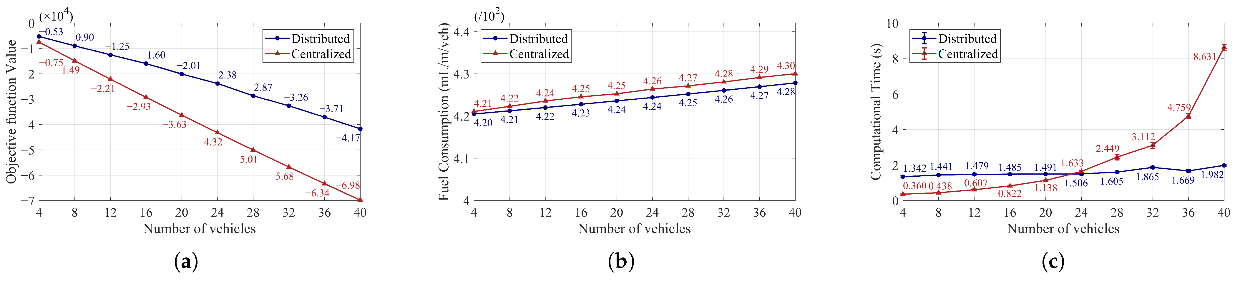
5.3. Impact of Vehicle Number in the Multi-Platoon Scenario 3

The impact of vehicle number in the multi-platoon scenario 3 is illustrated in Figure 14. As shown in Figure 14a, when the number of vehicles increases from 4 to 40, both methods show a clear drop in the objective function value. The same observations hold for both scenarios 1 and 2. Compared with the centralized method, the distributed method always shows higher objective function values, with differences increasing from 29.33% to 40.26% as the vehicle numbers grow. This is because the distributed method relies on local coordination that focuses on short-term speed improvements, while the centralized method uses a global strategy that better smooths acceleration.

The effect of increasing vehicle numbers on fuel consumption is shown in Figure 14b. When the platoon size grows from 4 to 40 vehicles, both methods show a slight rise in fuel consumption. The fuel consumption using the distributed method increases by 1.90%, and the centralized method by 2.14%. The centralized method consumes slightly more fuel than the distributed one, with a consistent difference of about 0.4%. This shows that global coordination in the centralized method forces more cautious speed changes, which slightly increases fuel use. However, the overall difference remains small.

The impact of computational time, as shown in Figure 14c, indicates that when the number of vehicles increases from 4 to 40, the computational time of the centralized method rises rapidly while the distributed method stays fairly stable. Similar observations are also found in scenarios 1 and 2. The centralized method works well for small platoons, but its computational performance suffers as platoon size grows, whereas the distributed method consistently maintains computational efficiency.

5.4. Control Performance Comparison Between the Single-Platoon Scenario 1 and Multi-Platoon Scenario 3

The control performance in the single-platoon scenario 1 and the multi-platoon scenario 3 is summarized and compared below. As shown in Figure 12a and Figure 14a, the objective function values obtained using the distributed method in the multi-platoon scenario 3 are generally 54.43% lower than those in the single-platoon scenario 1 with the same number of vehicles. When the number of vehicles increases, objective function values in scenario 1 decrease by 319.44%, while the counterparts in multi-platoon scenario 3 decrease by 349.06%. Furthermore, fuel consumption rises with an increase in the number of vehicles as seen in Figure 12b and Figure 14b. In scenario 1 (single-platoon), fuel consumption increases by 2.14%, while in scenario 3 (multi-platoon), it increases by 0.95%. Fuel consumption in the multi-platoon scenario remains consistently lower than the single-platoon scenario, and the difference widens from 0.24% to 1.40%. This is because multi-platoon collaboration helps avoid redundant decisions and reduce ineffective waiting times, whereas single-platoon systems, lacking cross-platoon coordination, concentrate all vehicles in one group, leading to congestion and resource waste.

The computational time in the single-platoon scenario 1 is generally higher than in the multi-platoon scenario 3. The centralized method has to manage complex decisions, causing exponential growth of computational time, while the distributed method shares the computational load by letting each platoon handle its own tasks. As illustrated in Figure 12c and Figure 14c, the differences in computational time using the distributed method between scenarios 1 and 3 are small (7.53%). However, using the centralized method, the difference in computation time increases to 40.73% with large vehicle numbers.

6. Conclusions

We designed a platoon trajectory controller to minimize travel time and ride discomfort by determining accelerations considering admissible motions and safe following gaps. To improve computational efficiency and information privacy, a distributed method is proposed here to decompose the coupling effects of safe inter-vehicle following gaps; therefore, each vehicle can independently solve its local tasks. The dual decomposition technique is applied to transform the coupled optimization problem into independent subproblems, allowing each vehicle to optimize its trajectory individually while satisfying overall platoon constraints. Proximal minimization iteratively updates the dual variables, ensuring convergence to the optimal solution. This distributed method effectively coordinates vehicle trajectories while preserving privacy in inter-vehicle communication as only local information is exchanged.

A series of simulation experiments were conducted to evaluate the control performance of the distributed method. The simulation results show the distributed controller can satisfy all control objectives and fulfill the controller constraints in single-platoon, multiple-platoon, and platoon-merging scenarios. The scalability of the distributed controller across different platoon sizes or the simulation horizons is also demonstrated. Compared with the centralized method, the proposed distributed method offers advantages in computational time and fuel consumption, while objective function values are slightly worse but remain within acceptable ranges. This improved performance mainly results from decomposing the global optimization into independent local subproblems, allowing parallel computation and reducing computational load as platoon size increases. The distributed method enables quick local trajectory adjustments, while the centralized method often requires multiple sequential updates, especially for tail vehicles, causing higher fuel consumption. By exchanging only essential information related to safe following gaps, the method preserves privacy without sacrificing coordination. These factors together enhance the efficiency and effectiveness of the distributed method.

Future work will focus on extending the approach to signalized intersections and urban networks, integrating traffic signal coordination to improve platoon performance in complex traffic scenarios. Lane-changing models will also be incorporated to combine longitudinal and lateral trajectory planning, enhancing adaptability to diverse traffic conditions. Additionally, energy consumption and emission considerations will be integrated into the framework to promote sustainable intelligent platoons.

References

1. Han, Y.; Wang, M.; Leclercq, L. Leveraging reinforcement learning for dynamic traffic control: A survey and challenges for field implementation. Commun. Transp. Res. 2023, 3, 100104. [Google Scholar] [CrossRef]
2. He, X.; Liu, H.X.; Liu, X. Optimal vehicle speed trajectory on a signalized arterial with consideration of queue. Transp. Res. Part C Emerg. Technol. 2015, 61, 106–120. [Google Scholar] [CrossRef]
3. Yang, K.; Guler, S.I.; Menendez, M. Isolated intersection control for various levels of vehicle technology: Conventional, connected, and automated vehicles. Transp. Res. Part C Emerg. Technol. 2016, 72, 109–129. [Google Scholar] [CrossRef]
4. Zhou, Q.; Zhou, B.; Hu, S.; Roncoli, C.; Wang, Y.; Hu, J.; Lu, G. A safety-enhanced eco-driving strategy for connected and autonomous vehicles: A hierarchical and distributed framework. Transp. Res. Part C Emerg. Technol. 2023, 156, 104320. [Google Scholar] [CrossRef]
5. Stebbins, S.; Hickman, M.; Kim, J.; Vu, H.L. Characterising green light optimal speed advisory trajectories for platoon-based optimisation. Transp. Res. Part C Emerg. Technol. 2017, 82, 43–62. [Google Scholar] [CrossRef]
6. Typaldos, P.; Papageorgiou, M. Modified dynamic programming algorithms for GLOSA systems with stochastic signal switching times. Transp. Res. Part C Emerg. Technol. 2023, 157, 104364. [Google Scholar] [CrossRef]
7. Yang, Z.; Zheng, Z.; Kim, J.; Rakha, H. Eco-driving strategies using reinforcement learning for mixed traffic in the vicinity of signalized intersections. Transp. Res. Part C Emerg. Technol. 2024, 165, 104683. [Google Scholar] [CrossRef]
8. Zhou, F.; Li, X.; Ma, J. Parsimonious shooting heuristic for trajectory design of connected automated traffic part I: Theoretical analysis with generalized time geography. Transp. Res. Part B Methodol. 2017, 95, 394–420. [Google Scholar] [CrossRef]
9. Ma, J.; Li, X.; Zhou, F.; Hu, J.; Park, B.B. Parsimonious shooting heuristic for trajectory design of connected automated traffic part II: Computational issues and optimization. Transp. Res. Part B Methodol. 2017, 95, 421–441. [Google Scholar] [CrossRef]
10. Yang, H.; Rakha, H.; Ala, M.V. Eco-cooperative adaptive cruise control at signalized intersections considering queue effects. IEEE Trans. Intell. Transp. Syst. 2016, 18, 1575–1585. [Google Scholar] [CrossRef]
11. Yang, X.T.; Huang, K.; Zhang, Z.; Zhang, Z.A.; Lin, F. Eco-driving system for connected automated vehicles: Multi-objective trajectory optimization. IEEE Trans. Intell. Transp. Syst. 2020, 22, 7837–7849. [Google Scholar] [CrossRef]
12. Nguyen, C.H.; Hoang, N.H.; Lee, S.; Vu, H.L. A system optimal speed advisory framework for a network of connected and autonomous vehicles. IEEE Trans. Intell. Transp. Syst. 2021, 23, 5727–5739. [Google Scholar] [CrossRef]
13. Hoang, A.T.; Nguyen, C.H.; Ngoduy, D.; Vu, H.L. Optimal trajectory planning framework for a mixed traffic network. In Proceedings of the 2022 IEEE 25th International Conference on Intelligent Transportation Systems (ITSC), Macau, China, 8–12 October 2022; pp. 2756–2762. [Google Scholar]
14. Wang, Y.; Li, J.; Ke, T.; Ke, Z.; Jiang, J.; Xu, S.; Wang, J. A homogeneous multi-vehicle cooperative group decision-making method in complicated mixed traffic scenarios. Transp. Res. Part C Emerg. Technol. 2024, 167, 104833. [Google Scholar] [CrossRef]
15. Ma, M.; Li, Z. A speed-maximization trajectory optimization model on a reservation-based intersection control system. Transp. Res. Part C Emerg. Technol. 2023, 154, 104266. [Google Scholar] [CrossRef]
16. Yao, H.; Li, X. Decentralized control of connected automated vehicle trajectories in mixed traffic at an isolated signalized intersection. Transp. Res. Part C Emerg. Technol. 2020, 121, 102846. [Google Scholar] [CrossRef]
17. Yao, S.; Zhou, Y.; Friedrich, B.; Ahn, S. Planning trajectories for connected and automated vehicle platoon on curved roads: A two-dimensional cooperative approach. Transp. Res. Part C Emerg. Technol. 2024, 165, 104718. [Google Scholar] [CrossRef]
18. Ma, C.; Yu, C.; Yang, X. Trajectory planning for connected and automated vehicles at isolated signalized intersections under mixed traffic environment. Transp. Res. Part C Emerg. Technol. 2021, 130, 103309. [Google Scholar] [CrossRef]
19. Zou, Y.; Zheng, F.; Liu, C.; Liu, X. Integrated optimization of traffic signals and vehicle trajectories for mixed traffic at signalized intersections: A two-level hierarchical control framework. Transp. Res. Part C Emerg. Technol. 2024, 169, 104884. [Google Scholar] [CrossRef]
20. Wang, J.; Lian, Y.; Jiang, Y.; Xu, Q.; Li, K.; Jones, C.N. Distributed data-driven predictive control for cooperatively smoothing mixed traffic flow. Transp. Res. Part C Emerg. Technol. 2023, 155, 104274. [Google Scholar] [CrossRef]
21. Wang, Q.; Gong, Y.; Yang, X. Connected automated vehicle trajectory optimization along signalized arterial: A decentralized approach under mixed traffic environment. Transp. Res. Part C Emerg. Technol. 2022, 145, 103918. [Google Scholar] [CrossRef]
22. Mohebifard, R.; Hajbabaie, A. Connected automated vehicle control in single lane roundabouts. Transp. Res. Part C Emerg. Technol. 2021, 131, 103308. [Google Scholar] [CrossRef]
23. Lei, Y.Z.; Cheng, Y.; Yang, X.T. An optimization-free approximation Framework for Connected and Automated Vehicles Eco-Trajectory Planning Under limited computing capacity. Transp. Res. Part C Emerg. Technol. 2025, 171, 104949. [Google Scholar] [CrossRef]
24. Falsone, A.; Margellos, K.; Garatti, S.; Prandini, M. Dual decomposition for multi-agent distributed optimization with coupling constraints. Automatica 2017, 84, 149–158. [Google Scholar] [CrossRef]
25. Falsone, A.; Margellos, K.; Prandini, M. A decentralized approach to multi-agent MILPs: Finite-time feasibility and performance guarantees. Automatica 2019, 103, 141–150. [Google Scholar] [CrossRef]
26. Falsone, A.; Margellos, K.; Prandini, M. A distributed iterative algorithm for multi-agent MILPs: Finite-time feasibility and performance characterization. IEEE Control. Syst. Lett. 2018, 2, 563–568. [Google Scholar] [CrossRef]
27. Zhou, J.; Zhu, F. Analytical analysis of the effect of maximum platoon size of connected and automated vehicles. Transp. Res. Part C Emerg. Technol. 2021, 122, 102882. [Google Scholar] [CrossRef]
28. Li, S.; Zheng, H.; Wang, J.; Chen, C.; Xu, Q.; Wang, J.; Li, K. Influence of information flow topology and maximum platoon size on mixed traffic stability. Transp. Res. Part C Emerg. Technol. 2025, 171, 104950. [Google Scholar] [CrossRef]
29. Sánchez, M.M.; van der Ploeg, C.; Smit, R.; Elfring, J.; Silvas, E.; van de Molengraft, R. Prediction horizon requirements for automated driving: Optimizing safety, comfort, and efficiency. In Proceedings of the 2024 IEEE Intelligent Vehicles Symposium (IV), Jeju Island, Republic of Korea, 2–5 June 2024; pp. 2575–2582. [Google Scholar]
30. Bai, T.; Johansson, A.; Johansson, K.H.; Mårtensson, J. Large-scale multi-fleet platoon coordination: A dynamic programming approach. IEEE Trans. Intell. Transp. Syst. 2023, 24, 14427–14442. [Google Scholar] [CrossRef]
31. Zhao, W.; Yildirimoglu, M. A scalable macro–micro approach for cooperative platoon merging in mixed traffic flows. Transp. Res. Part C Emerg. Technol. 2024, 169, 104859. [Google Scholar] [CrossRef]
32. Kamal, M.A.S.; Mukai, M.; Murata, J.; Kawabe, T. Model predictive control of vehicles on urban roads for improved fuel economy. IEEE Trans. Control. Syst. Technol. 2012, 21, 831–841. [Google Scholar] [CrossRef]
Figure 1. Trajectories of movement under scenario 1: (a) distributed method; (b) centralized method.
Systems 13 00483 g001
Figure 2. Speed of movement under scenario 1: (a) distributed method; (b) centralized method.
Systems 13 00483 g002
Figure 3. Space gap of movement under scenario 1: (a) distributed method; (b) centralized method.
Systems 13 00483 g003
Figure 4. Acceleration of movement under scenario 1: (a) distributed method; (b) centralized method.
Systems 13 00483 g004
Figure 5. Speed of movement under scenario 2: (a) distributed method; (b) centralized method.
Systems 13 00483 g005
Figure 6. Acceleration of movement under scenario 2: (a) distributed method; (b) centralized method.
Systems 13 00483 g006
Figure 7. Trajectories of movement under scenario 3: (a) distributed method; (b) centralized method.
Systems 13 00483 g007
Figure 8. Speed of movement under scenario 3: (a) distributed method; (b) centralized method.
Systems 13 00483 g008
Figure 9. Gap of movement under scenario 3: (a) distributed method; (b) centralized method.
Systems 13 00483 g009
Figure 10. Trajectories of movement under scenario 4: (a) distributed method; (b) centralized method.
Systems 13 00483 g010
Figure 11. Gap of movement under scenario 4: (a) distributed method; (b) centralized method.
Systems 13 00483 g011
Figure 12. Comparison of distributed and centralized systems under scenario 1: (a) objective function value; (b) fuel consumption; (c) computational time.
Systems 13 00483 g012
Figure 13. Comparison of distributed and centralized systems under scenario 2: (a) objective function value; (b) fuel consumption; (c) computational time.
Systems 13 00483 g013
Figure 14. Comparison of distributed and centralized systems under scenario 3: (a) objective function value; (b) fuel consumption; (c) computational time.
Systems 13 00483 g014