
Effect of Pre-Trip Information in a Traffic Network with Stochastic Travel Conditions: Role of Risk Attitude

Abstract
1. Introduction
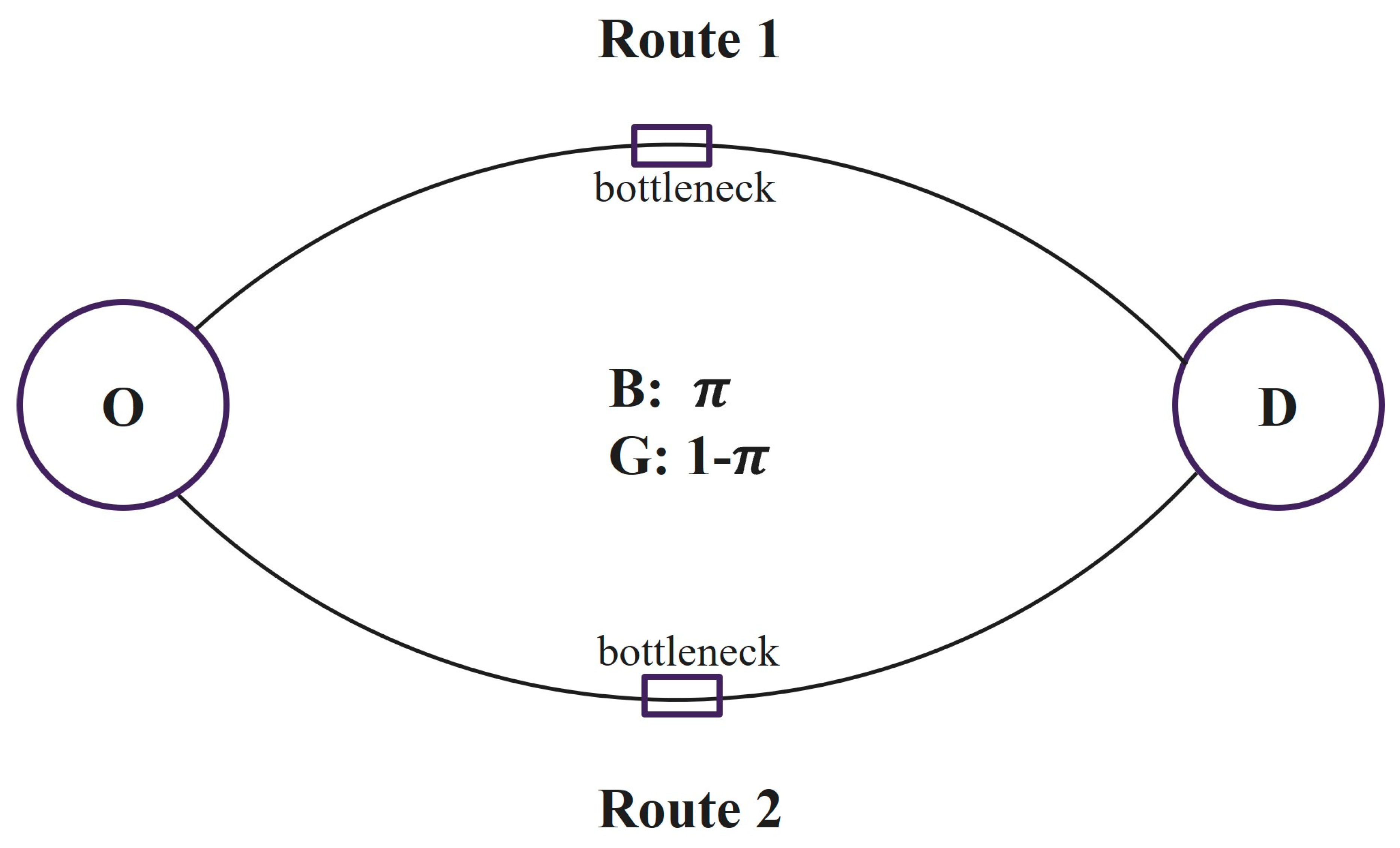
2. The Model
3. User Equilibrium
3.1. User Equilibrium in the Zero-Information Regime
3.1.1. Three Scenarios Under
- Scenario A:
- 2.
- Scenario B: and
- 3.
- Scenario C: and
3.1.2. Closed Form UE Solutions Under
- 1.
- Situations (i) and (ii)
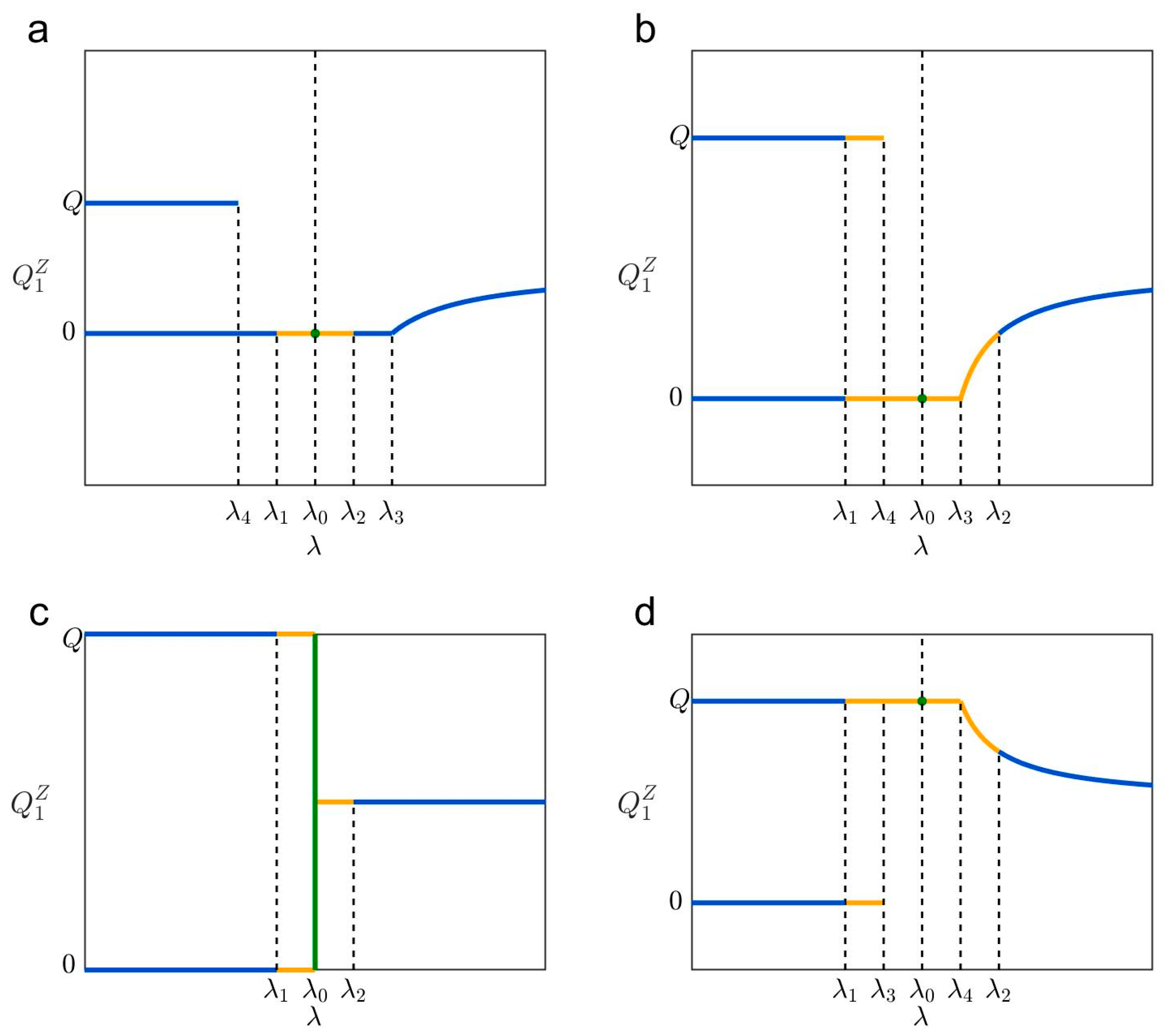
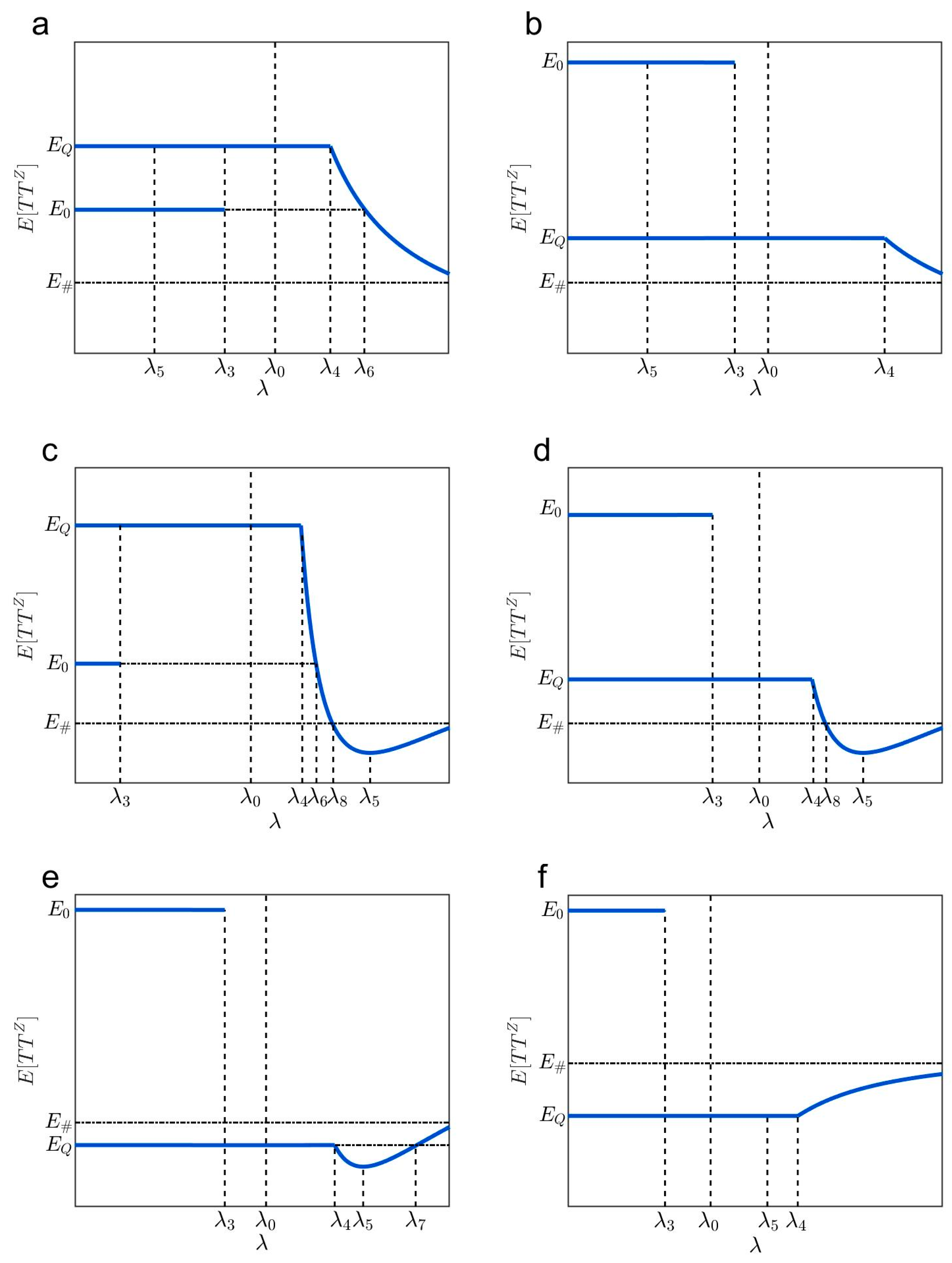
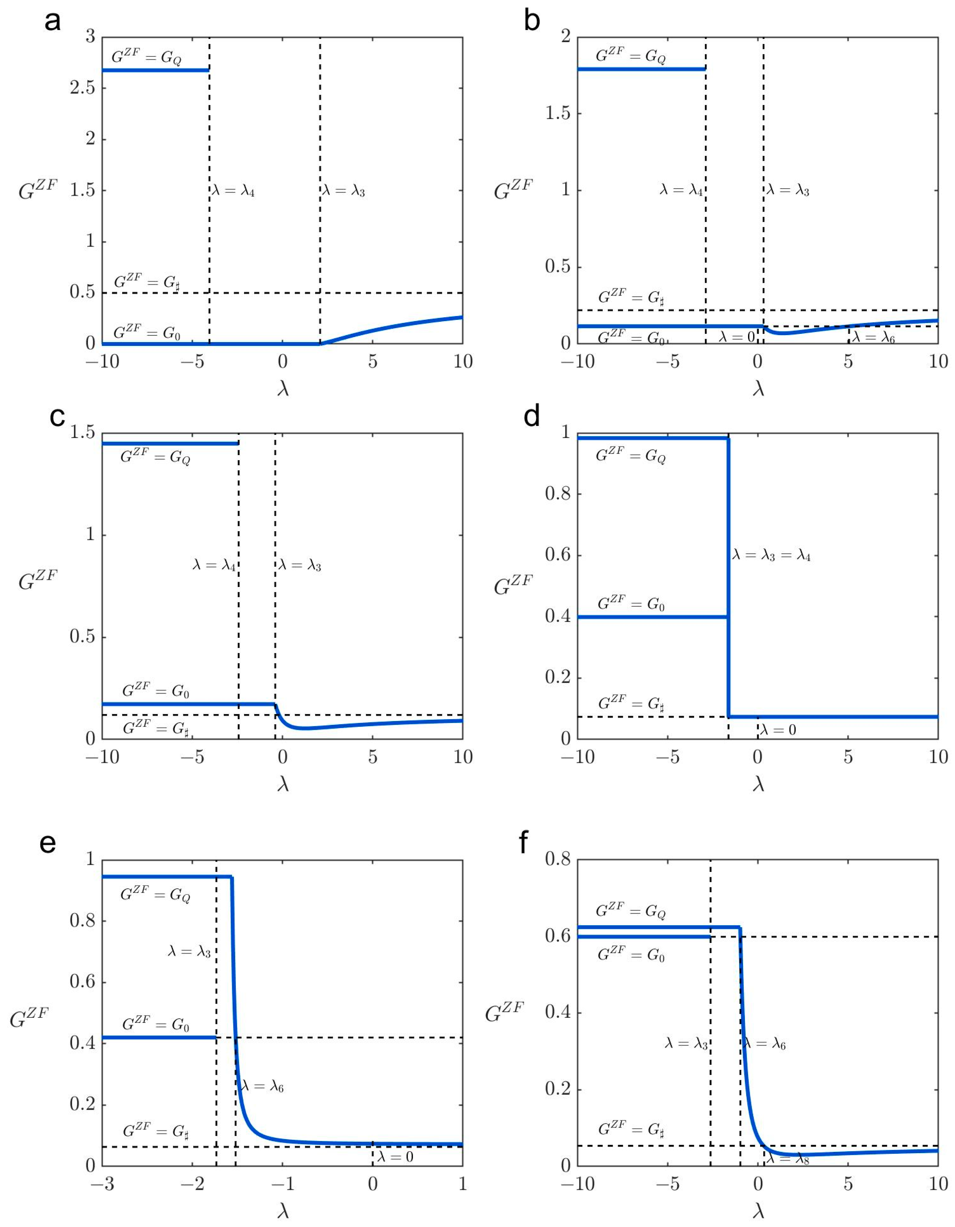
- Situation (i) corresponds to and (see Figure 5a). In this situation, patterns C1, C2, B2, B6, C6, and C4 exist when the risk attitude belongs to , , , , , and , respectively.
- Situation (ii) corresponds to and (see Figure 5b). In this situation, patterns C1, B1, B2, B6, B4, and C4 exist when belongs to , , , , , and , respectively.
- Note that when , , and cannot be not met simultaneously, and cannot be not met simultaneously, either.
- 2.
- Situation (iii)
- 3.
- Situations (iv)–(vii)
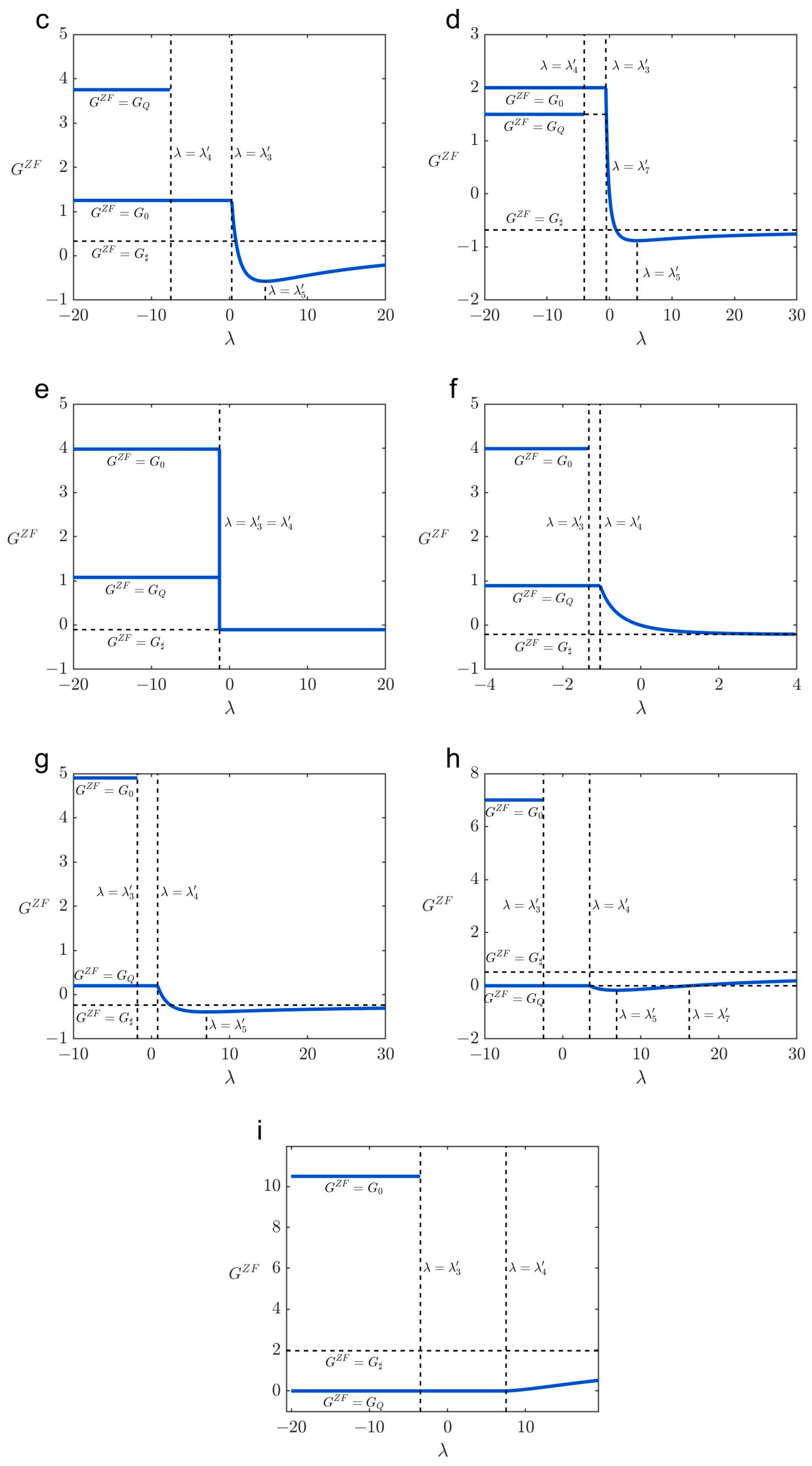
- Situation (iv) corresponds to and (see Figure 5d). In this situation, patterns C1, B1, B3, B5, B4, and C4 exist when belongs to , , , , , and , respectively.
- Situation (v) corresponds to and (see Figure 5e). In this situation, patterns C1, B1, B3, B5, C5, and C4 exist when belongs to , , , , , and , respectively.
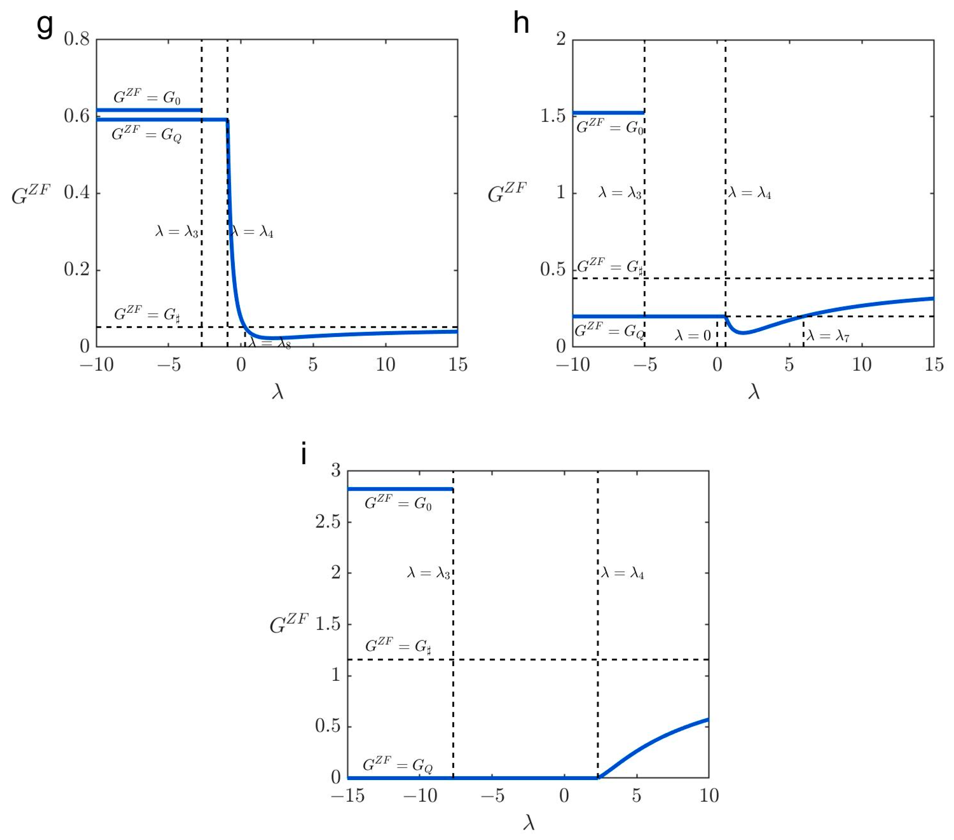
- Situation (vi) corresponds to and (see Figure 5f). In this situation, patterns C1, C3, B3, B5, B4, and C4 exist when belongs to , , , , , and , respectively.
- Situation (vii) corresponds to and (see Figure 5g). In this situation, patterns C1, C3, B3, B5, C5, and C4 exist when belongs to , , , , , and , respectively.
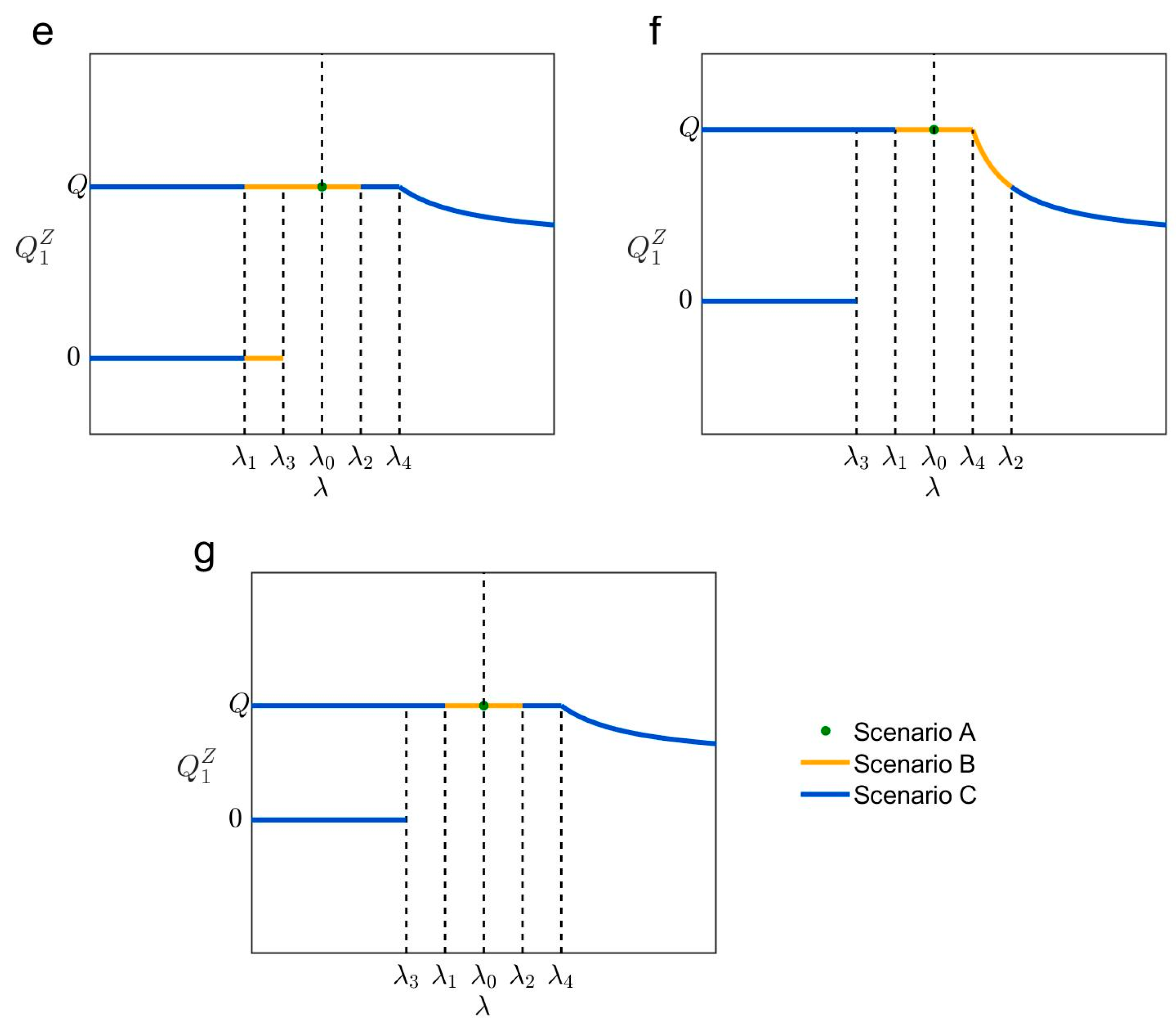
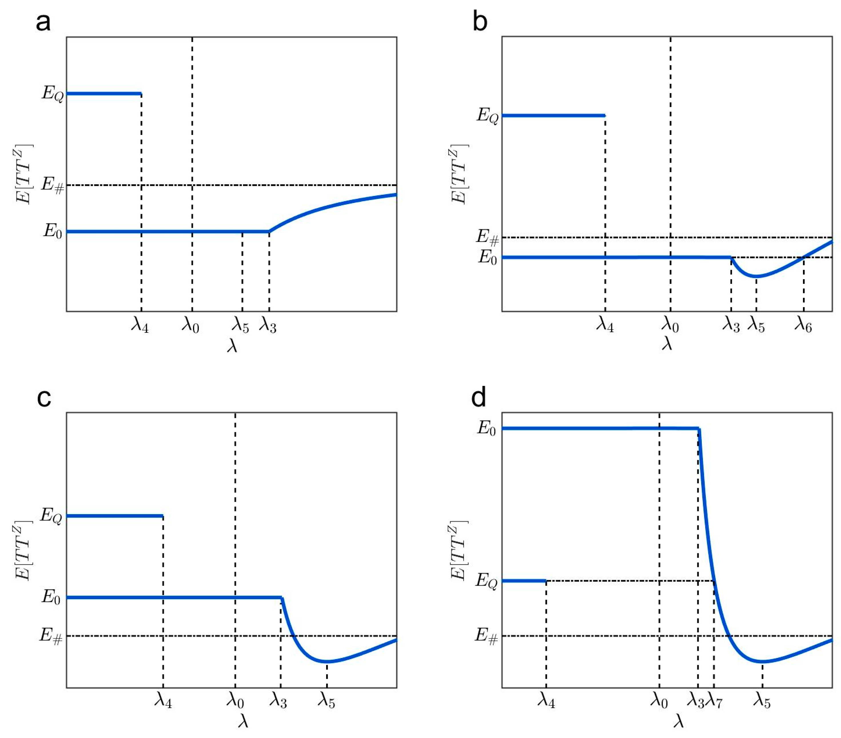
- Case 1 in Figure 6a–d: When , case 1 exists. One can easily prove that and are always met in case 1. Case 1 can be further classified into cases 1a–1d.
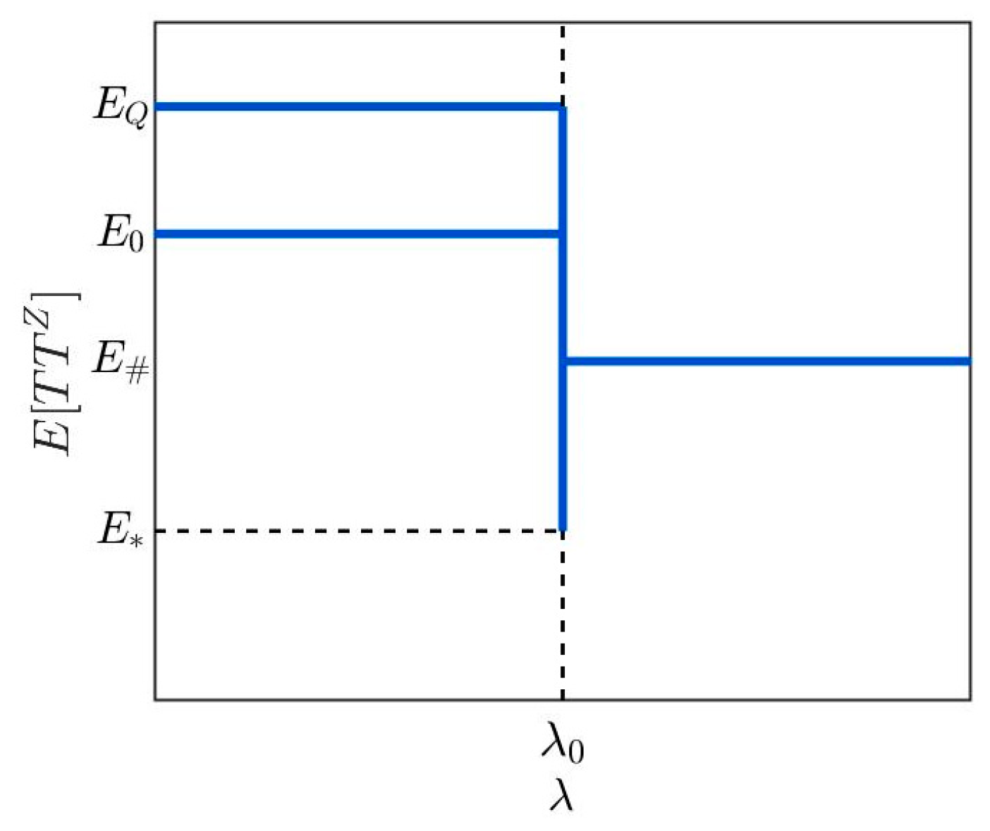
- Case 2 in Figure 7: When , case 2 exists. One can easily prove that and are always met in case 2. In this case, there are two possible UE states when ; the expected total travel time is not uniquely determined when , which can be any value between and . Here,which denotes the minimum value of the expected total travel time. Note that is met due to . Finally, is a constant no matter what the risk attitude is when , which can be calculated,
- Case 3 in Figure 8a–f: When , case 3 exists. One can easily prove that and are always met in case 3. Case 3 can be further classified into cases 3a–3f.
3.1.3. General Results Under
- (a)
- when , if the functions and are identical, the state is a UE state; otherwise, the two functions are a tangent at , which is not a UE state, unless (if is above ) or (if is below );
- (b)
- when , the state is not a UE state;
- (c)
- when , the state is a UE state.
- (a)
- when , there are two possible UE states ( or ) when . Otherwise, a unique UE state exists: when ; and increases with when ;
- (b)
- when , there are two possible UE states ( or ) when ; the UE traffic demand is not uniquely determined, which can be any value between 0 and () when ; the UE traffic demand is a constant when ;
- (c)
- when , there are two possible UE states ( or ) when . Otherwise, a unique UE state exists: when ; ; and decreases with when .
3.2. User Equilibrium in the Full-Information Regime
- (a)
- when , all travelers choose route 2 under UE (i.e., );
- (b)
- when , the UE state is ();
- (c)
- when , all travelers choose route 1 under UE (i.e., ).
4. Welfare Gains or Losses from Information
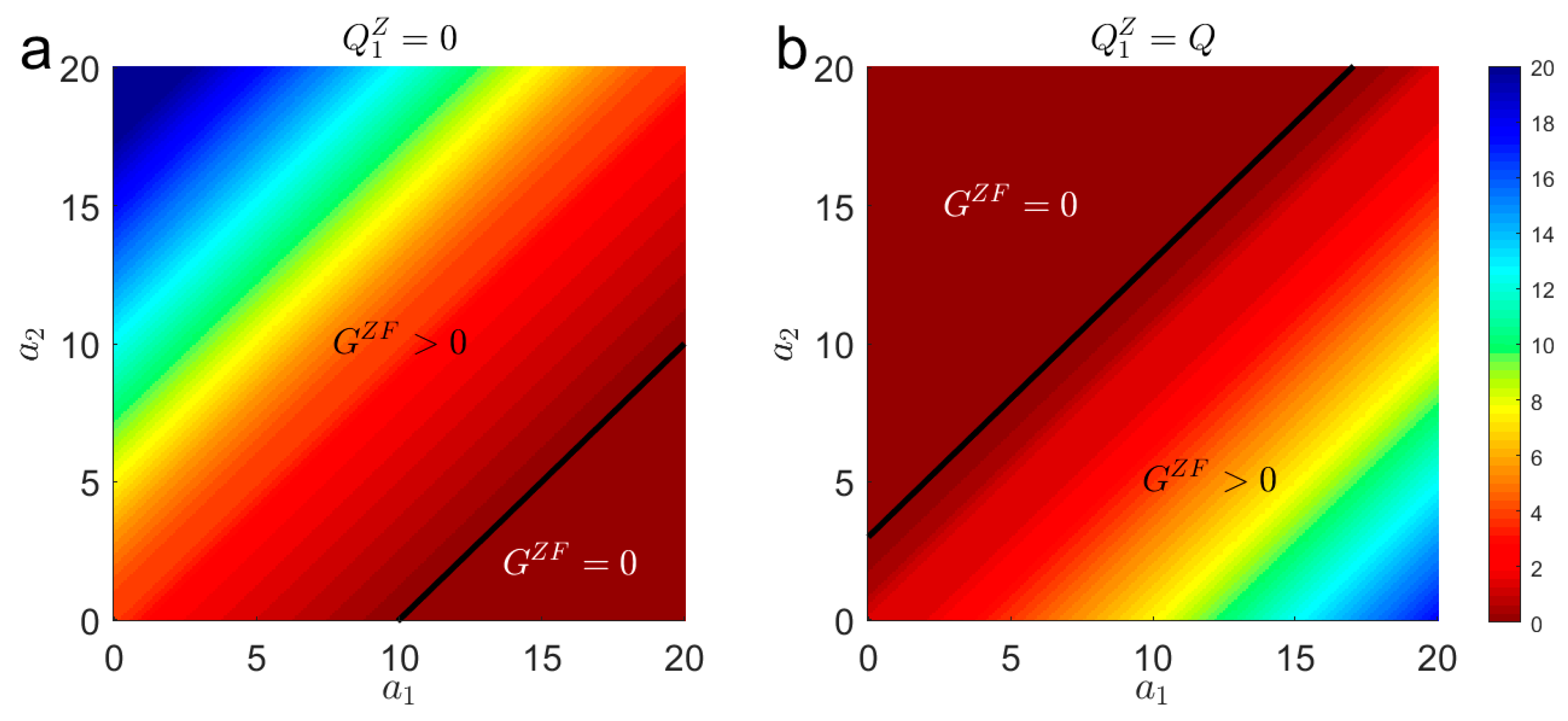
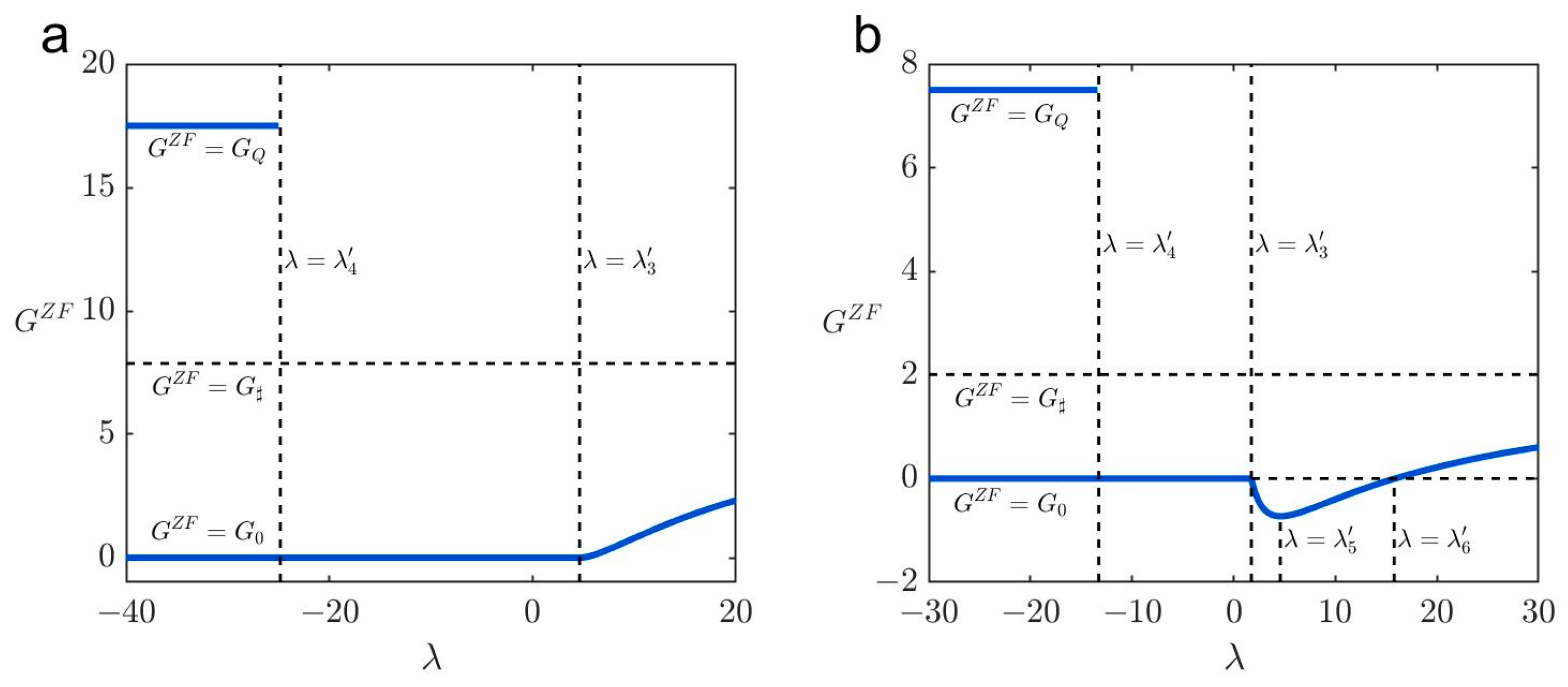
- (a)
- when in either case 1c or case 2;
- (b)
- when in either case 3b or case 3d;
- (c)
- when in either case 3a or case 3c;
- (d)
- when in case 1d;
- (e)
- when or in case 1b;
- (f)
- when or in case 3e.
- (a)
- In case 3a and case 3c, risk-neutral travelers obtain no more welfare gains than risk-preferred ones with risk attitude ;
- (b)
- In case 1d, risk-neutral travelers obtain no more welfare gains than risk-preferred ones with risk attitude .
- (a)
- In case 1b, risk-neutral travelers obtain no more welfare gains than risk-averse ones with risk attitude ;
- (b)
- In case 3e, risk-neutral travelers obtain no more welfare gains than risk-averse ones with risk attitude .
- (a)
- In case 3c and case 3d, risk-neutral travelers obtain more welfare gains than risk-averse ones with risk attitude ;
- (b)
- In case 3e, risk-neutral travelers obtain more welfare gains than risk-averse ones with risk attitude .
5. Numerical Analysis
5.1. The Effect of Pre-Trip Information in the General Condition
5.2. The Effect of Pre-Trip Information in the Special Case
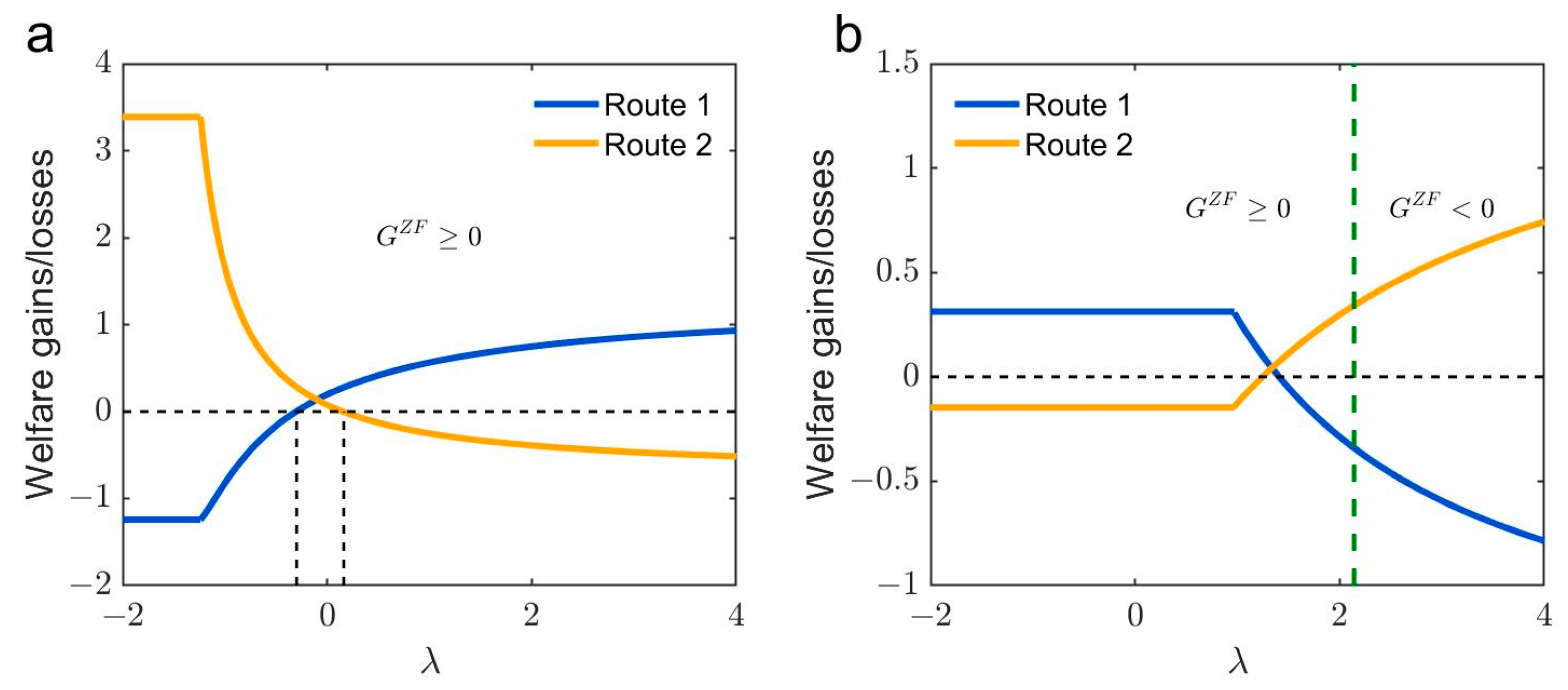
5.3. The Effect of Pre-Trip Information on Different Routes
6. Conclusions and Discussion
Author Contributions
Funding
Data Availability Statement
Conflicts of Interest
Appendix A
Appendix A.1. Proof of Proposition 2
- (a)
- The function is an increasing one of . Substituting into the equation , one has
- (b)
- The function is an increasing one of . By solving , one has . Substituting and into , one has and , respectively. Therefore, is a decreasing function of when and an increasing function when .
- (1)
- . In this case, one has . When , one has , in which and , so that . When , one has , in which and , so that . Therefore, the function is an increasing one of for the two branches. Moreover, when (or ), one has (or ), because the function is continuous, except at . As a result, three possible subcases need to be classified.
- -
- When , one can easily prove that is always met; thereby, is a UE state. However, according to Property 1(b), the solution is not a UE state, because is always met when ;
- -
- When , one can easily prove that is always met. Thereby, is a UE state;
- -
- When , it is obvious that or is not a UE state; however, according to Property 1(c), the solution is a UE state, because is always met when .
- (2)
- . In this case, one has . It is straightforward to prove that is always met, so that for an arbitrary , in which is a constant (), no matter what the risk attitude is. As a result, three possible subcases need to be classified.
- -
- . According to Property 1(b), the solution is not a UE state because ; similar to the analysis above, there are two possible UE states, or ;
- -
- . According to Property 1(c), the solution is a UE state, because ;
- -
- . In this subcase, is always met when . Substituting into , one has . Thus, we have , because . As a result, the functions and are identical. According to Property 1(a), is not uniquely determined, which can be any value between 0 and ().
- (3)
- . In this case, one has . When , one has , in which and , so that . When , one has , in which and , so that . Therefore, the function is a decreasing one of for the two branches. Moreover, when (or ), one has (or ), because the function is continuous except at . Similar to the analysis above, three possible subcases need to be classified:
- -
- when , one can easily prove that is always met. Thus, is a UE state; however, according to Property 1(b), the solution is not a UE state, because is always met when ;
- -
- when , one can easily prove that is always met. Thus, is a UE state;
- -
- when , it is obvious that or is not a UE state; however, according to Property 1(c), the solution is a UE state because is always met when .
Appendix A.2. Proof of Proposition 3
Appendix A.3. Proof of Proposition 4
- (1)
- when , it is clear that is a UE state and is not a UE state. Substituting and into Equation (34), one has
- (2)
- when , it is clear that is a UE state and is not a UE state. Substituting and into Equation (34), one has
- (3)
- when , it is clear that neither nor is a UE state. Assume that the slopes of functions and under the solution are
Appendix A.4. Proof of Proposition 5
- (a)
- If , together with (Assumption 1), one can easily derive that all travelers choose route 1 under UE, i.e., . Substituting into Equation (32), one has
- (b)
- If , then one has and . Substituting into Equation (32), one has
- (c)
- If , then one has . Substituting into Equation (32), one has
References
- Levinson, D. The value of advanced traveler information systems for route choice. Transp. Res. Part C Emerg. Technol. 2003, 11, 75–87. [Google Scholar] [CrossRef]
- Luo, X.; Liu, Y.; Yu, Y. Dynamic bus dispatching using multiple types of real-time information. Transp. B Transp. Dyn. 2019, 7, 519–545. [Google Scholar] [CrossRef]
- Mori, U.; Mendiburu, A.; Alvarez, M.; Lozano, J.A. A review of travel time estimation and forecasting for advanced traveler information systems. Transp. A Transp. Sci. 2015, 11, 119–157. [Google Scholar]
- Neil, L.; Richard, H.; Jeff, H. Driver opinion of message requirements for advanced traveler information systems. Plant Physiol. 1970, 45, 576–578. [Google Scholar]
- Perez, W.A.; Mast, T.M. Human factors and advanced traveler information systems (ATIS). Proc. Hum. Factors Ergon. Soc. Annu. Meet. 1992, 36, 1073–1077. [Google Scholar] [CrossRef]
- Rapoport, A.; Gisches, E.J.; Daniel, T.; Lindsey, R. Pre-trip information and route-choice decisions with stochastic travel conditions: Experiment. Transp. Res. Part B Methodol. 2014, 68, 154–172. [Google Scholar] [CrossRef]
- Sen, S.; Pillai, R.; Joshi, S.; Rathi, A.K. A mean-variance model for route guidance in advanced traveler information systems. Transp. Sci. 2001, 35, 37–49. [Google Scholar] [CrossRef]
- Emmerink, R.H.M.; Nijkamp, P.; Rietveld, P.; Van Ommeren, J.N. Variable message signs and radio traffic information: An integrated empirical analysis of drivers’ route choice behavior. Transp. Res. Part A Policy Pract. 1996, 30, 135–153. [Google Scholar] [CrossRef]
- Li, M.; Lin, X.; He, F.; Jiang, H. Optimal locations and travel time display for variable message signs. Transp. Res. Part C Emerg. Technol. 2016, 69, 418–435. [Google Scholar] [CrossRef]
- Wang, C.; David, B.; Chalon, R. Dynamic road lane management study. Transp. Res. Part E Logist. Transp. Rev. 2016, 89, 272–287. [Google Scholar] [CrossRef]
- Yu, Y.; Machemehl, R.B.; Xie, C. Demand-responsive transit circulator service network design. Transp. Res. Part E Logist. Transp. Rev. 2015, 76, 160–175. [Google Scholar] [CrossRef]
- Ahmed, A.; Ngoduy, D.; Watling, D. Prediction of traveller information and route choice based on real-time estimated traffic state. Transp. B Transp. Dyn. 2016, 4, 23–47. [Google Scholar] [CrossRef]
- Ben-Elia, E.; Avineri, E. Response to travel information: A behavioral review. Transp. Rev. 2015, 35, 352–377. [Google Scholar] [CrossRef]
- Chorus, C.G.; Eric JE, M.; van Wee, B. Travel information as an instrument to change car drivers’ travel choices: A literature review. Eur. J. Transp. Infrastruct. Res. 2006, 6, 335–364. [Google Scholar]
- Chorus, C.G.; Arentze, T.A.; Timmermans, H.J.P. Traveler compliance with advice: A Bayesian utilitarian perspective. Transp. Res. Part E Logist. Transp. Rev. 2009, 45, 486–500. [Google Scholar] [CrossRef]
- Golob, T.F.; Regan, A.C. The perceived usefulness of different sources of traffic information to trucking operations. Transp. Res. Part E Logist. Transp. Rev. 2002, 38, 97–116. [Google Scholar] [CrossRef]
- Los, J.; Schulte, F.; Spaan, M.T.J. The Value of Information Sharing for Platform-Based Collaborative Vehicle Routing. Transp. Res. Part E Logist. Transp. Rev. 2020, 141, 102011. [Google Scholar] [CrossRef]
- Wepulanon, P.; Sumalee, A.; Lam, W.H.K. A real-time bus arrival time information system using crowdsourced smartphone data: A novel framework and simulation experiments. Transp. B 2017, 6, 34–53. [Google Scholar] [CrossRef]
- Zhu, Z.; Li, X.W.; Liu, W.; Yang, H. Day-to-day evolution of departure time choice in stochastic capacity bottleneck models with bounded rationality and various information perceptions. Transp. Res. Part E Logist. Transp. Rev. 2019, 131, 168–192. [Google Scholar] [CrossRef]
- Ben-Elia, E.; Pace, R.D.; Bifuico, G.N. The impact of travel information’s accuracy on route-choice. Transp. Res. Part C Emerg. Technol. 2013, 26, 146–159. [Google Scholar] [CrossRef]
- Engelson, L.; Fosgerau, M. Scheduling preferences and the value of travel time information. Transp. Res. Part B Methodol. 2020, 134, 256–265. [Google Scholar] [CrossRef]
- Khattak, A.J.; Yim, Y.; Prokopy, L.S. Willingness to pay for travel information. Transp. Res. Part C Emerg. Technol. 2003, 11, 137–159. [Google Scholar] [CrossRef]
- Mahmassani, H.S.; Chee, C.T. Availability of information and dynamics of departure time choices: Experimental investigation. Transp. Res. Rec. J. Transp. Res. Board 1986, 1085, 33–49. [Google Scholar]
- Emmerink, R.H.M.; Kay, W.A.; Peter, N.; Piet, R. The potential of information provision in a simulated road transport network with non-recurrent congestion. Transp. Res. Part C Emerg. Technol. 1995, 3, 293–309. [Google Scholar] [CrossRef]
- Acemoglu, D.; Makhdoumi, A.; Malekian, A.; Ozdaglar, A. Informational braess’ paradox: The effect of information on traffic congestion. Oper. Res. 2016, 66, 893–917. [Google Scholar] [CrossRef]
- Emmerink, R.H.M.; Verhoef, E.T.; Nijkamp, P.; Rietveld, P. Information policy in road transport with elastic demand: Some welfare economic considerations. Eur. Econ. Rev. 1998, 42, 71–95. [Google Scholar] [CrossRef]
- Verhoef, E.T.; Emmerink, R.H.M.; Nijkamp, P.; Rietveld, P. Information provision, flat and fine congestion tolling and the efficiency of road usage. Reg. Sci. Urban Econ. 1996, 26, 505–529. [Google Scholar] [CrossRef]
- Lindsey, R.; Daniel, T.; Gisches, E.J.; Rapoport, A. Pre-trip information and route-choice decisions with stochastic travel conditions: Theory. Transp. Res. Part B Methodol. 2014, 67, 187–207. [Google Scholar] [CrossRef]
- Abdel-Aty, M.A.; Kitamura, R.; Jovanis, P.P. Investigating effect of travel time variability on route choice using repeated-measurement stated preference data. Transp. Res. Rec. 1995, 1493, 39–45. [Google Scholar]
- Jackson, W.B.; Jucker, J.V. An empirical study of travel time variability and travel choice behavior. Transp. Sci. 1982, 16, 460–475. [Google Scholar] [CrossRef]
- Chen, A.; Zhou, Z. The α-reliable mean-excess traffic equilibrium model with stochastic travel times. Transp. Res. Part B Methodol. 2010, 44, 493–513. [Google Scholar] [CrossRef]
- Chen, A.; Zhou, Z.; Lam, W.H.K. Modeling stochastic perception error in the mean-excess traffic equilibrium model. Transp. Res. Part B Methodol. 2011, 45, 1619–1640. [Google Scholar] [CrossRef]
- Xu, X.; Chen, A.; Cheng, L. Assessing the effects of stochastic perception error under travel time variability. Transportation 2013, 40, 525–548. [Google Scholar] [CrossRef]
- Xu, X.; Chen, A.; Cheng, L.; Lo, H.K. Modeling distribution tail in network performance assessment: A mean-excess total travel time risk measure and analytical estimation method. Transp. Res. Part B Methodol. 2014, 66, 32–49. [Google Scholar] [CrossRef]
- Zhou, Z.; Chen, A. Comparative analysis of three user equilibrium models under stochastic demand. J. Adv. Transp. 2008, 42, 239–263. [Google Scholar] [CrossRef]
- Lo, H.K.; Tung, Y.K. Network with degradable links: Capacity analysis and design. Transp. Res. Part B Methodol. 2003, 37, 345–363. [Google Scholar] [CrossRef]
- Lo, H.K.; Luo, X.W.; Siu, B.W.Y. Degradable transport network: Travel time budget of travelers with heterogeneous risk aversion. Transp. Res. Part B Methodol. 2006, 40, 792–806. [Google Scholar] [CrossRef]
- Yin, Y.; Lam, W.H.K.; Ieda, H. New technology and the modeling of risk-taking behavior in congested road networks. Transp. Res. Part C 2004, 12, 171–192. [Google Scholar] [CrossRef]
- Tan, Z.; Yang, H.; Guo, R. Pareto efficiency of reliability-based traffic equilibria and risk-taking behavior of travelers. Transp. Res. Part B Methodol. 2014, 66, 16–31. [Google Scholar] [CrossRef]
- Li, Z. Unobserved and observed heterogeneity in risk attitudes: Implications for valuing travel time savings and travel time variability. Transp. Res. Part E Logist. Transp. Rev. 2018, 112, 12–18. [Google Scholar] [CrossRef]
- U.S. Bureau of Public Roads. Traffic Assignment Manual; U.S. Bureau of Public Roads: Washington, DC, USA, 1964.

| Variable | Description |
|---|---|
| full-information regime | |
| zero-information regime | |
| index of route | |
| bad condition | |
| good condition | |
| possible condition | |
| possible condition on route 2 | |
| Set of conditions, | |
| free-flow travel time on route i | |
| stochastic congestion coefficient on route i when it is in state s | |
| total traffic demand | |
| traffic demand on route i | |
| traffic demand on route i when route 1 is in state s and route 2 is in state in the full-information regime | |
| travel time function on route i when it is in state s | |
| expectations operator | |
| travel time on route i | |
| total travel time on the network | |
| total travel time on route i | |
| total travel time on the network when route 1 is in state s and route 2 is in state | |
| the expected travel time on route i in the zero-information regime | |
| the expected total travel time in the zero-information regime | |
| the expected total travel time in the full-information regime | |
| travel time budget on route i in the zero-information regime | |
| the variance of in the zero-information regime | |
| risk-preference coefficient of travelers | |
| degradation probability of capacity () | |
| threshold of , h = 0, 1, 2, …, 8 in the special case | |
| threshold of , h = 0, 1, 2, …, 8 in the general condition | |
| three different thresholds of | |
| welfare gains (losses) from pre-trip information | |
| Pattern | Existence Condition | Main Characteristics | UE State | Example |
|---|---|---|---|---|
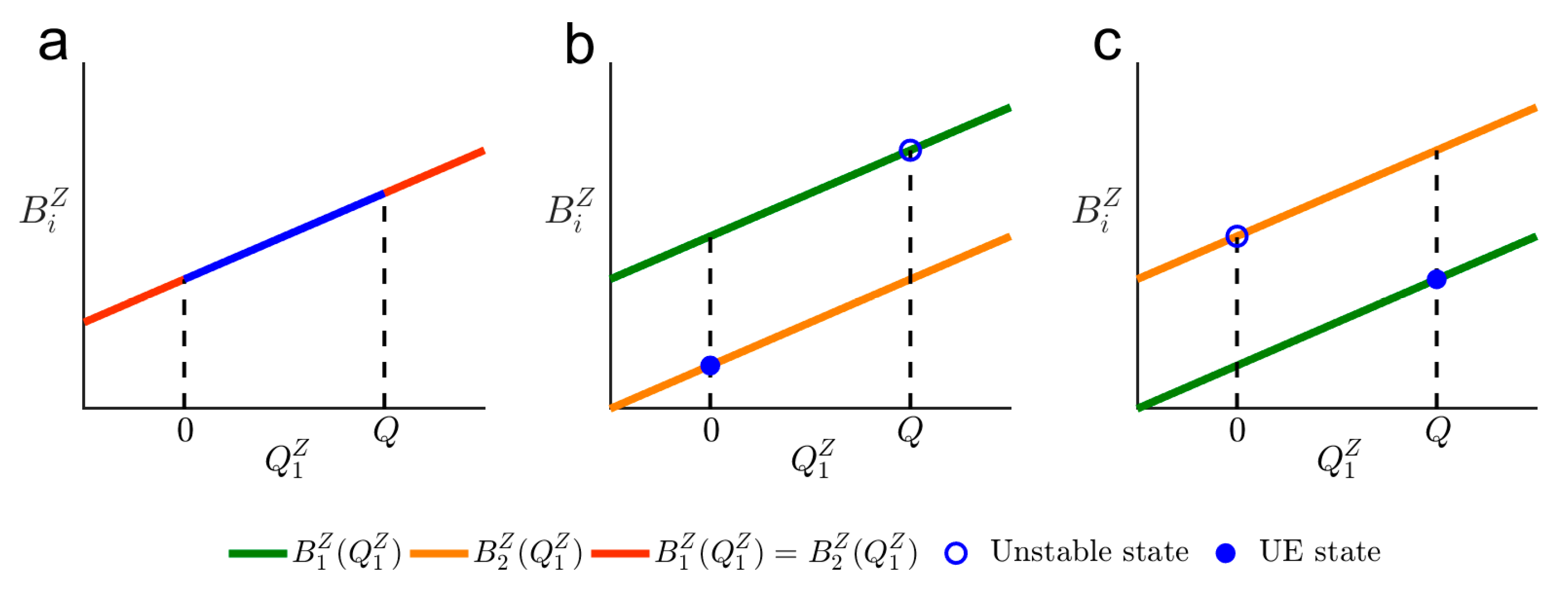
| A1 | are identical | Figure 2a | ||
| A2 | Figure 2b | |||
| A3 | Figure 2c |
| Pattern | Existence Condition | UE State | Example | |
|---|---|---|---|---|
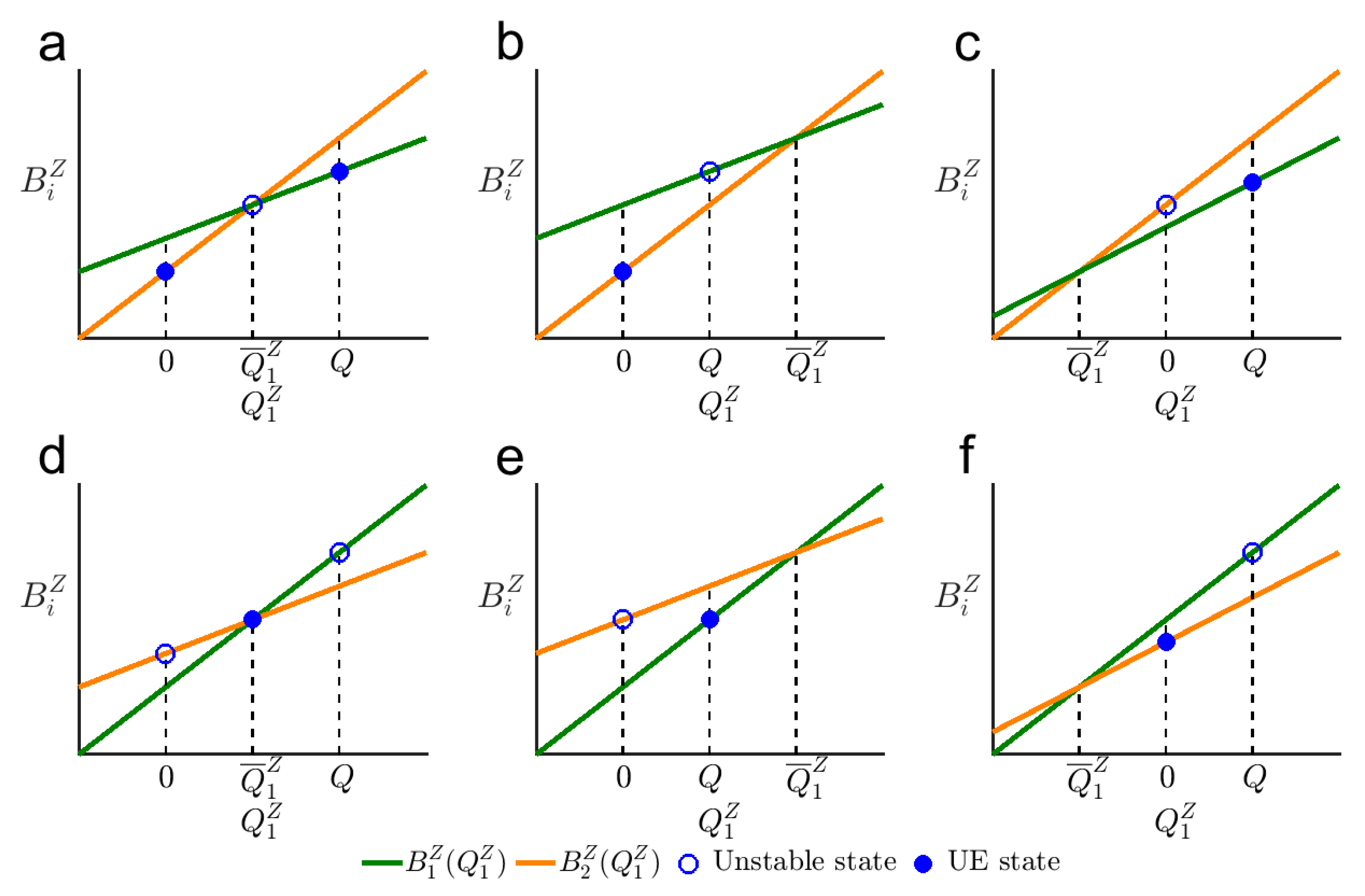
| B1 | Figure 3a | |||
| B2 | Figure 3b | |||
| B3 | Figure 3c | |||
| B4 | 0 < < Q | = | Figure 3d | |
| B5 | Figure 3e | |||
| B6 | Figure 3f | |||
| Pattern | Existence Condition | UE State | Example | |
|---|---|---|---|---|
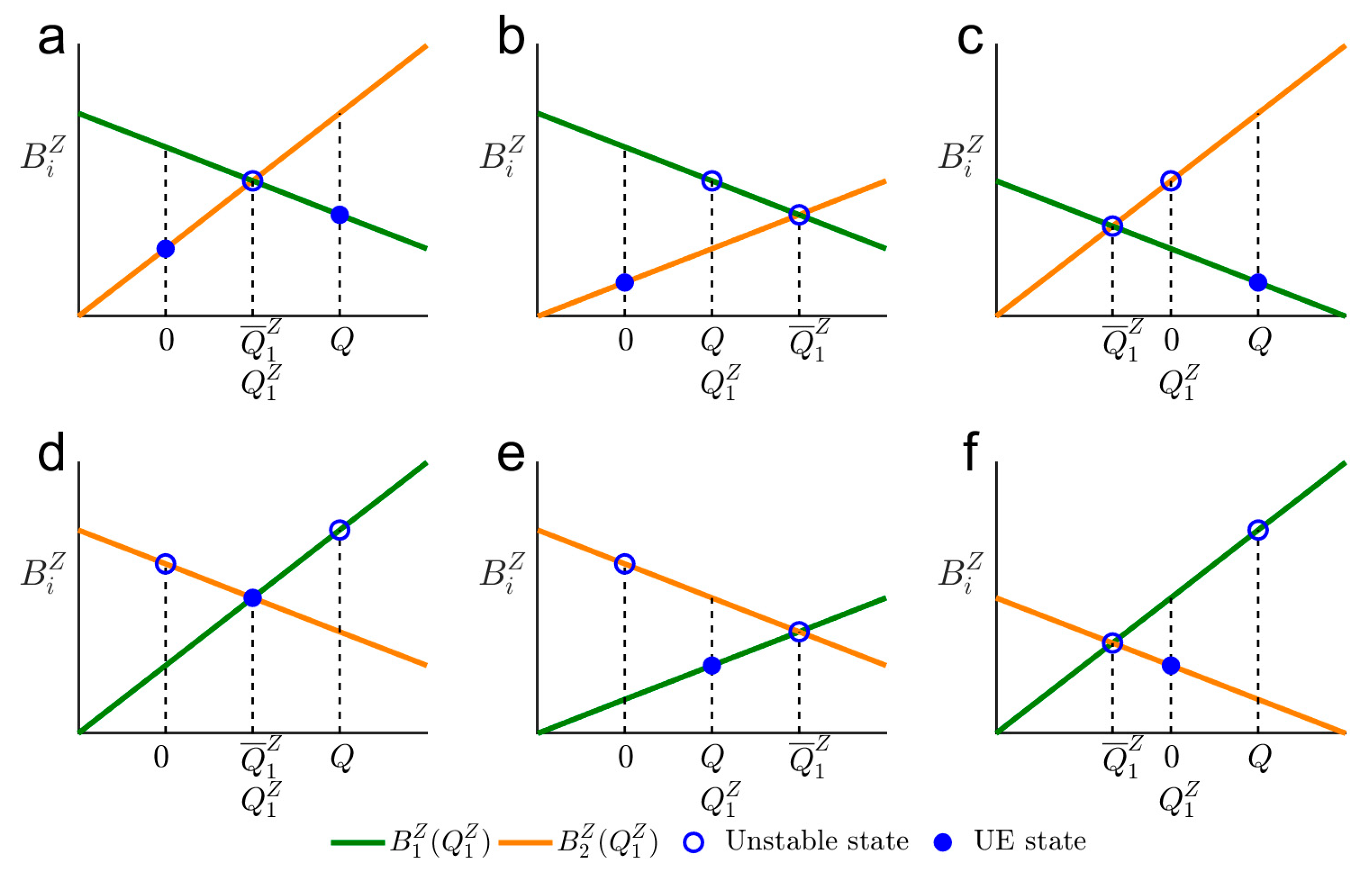
| C1 | Figure 4a | |||
| C2 | Figure 4b | |||
| C3 | Figure 4c | |||
| C4 | Figure 4d | |||
| C5 | Figure 4e | |||
| C6 | Figure 4f | |||
Disclaimer/Publisher’s Note: The statements, opinions and data contained in all publications are solely those of the individual author(s) and contributor(s) and not of MDPI and/or the editor(s). MDPI and/or the editor(s) disclaim responsibility for any injury to people or property resulting from any ideas, methods, instructions or products referred to in the content. |
© 2025 by the authors. Licensee MDPI, Basel, Switzerland. This article is an open access article distributed under the terms and conditions of the Creative Commons Attribution (CC BY) license (https://creativecommons.org/licenses/by/4.0/).
Share and Cite
Yu, Y.; Zheng, S.; Li, Y.; Liu, H.; Cao, J. Effect of Pre-Trip Information in a Traffic Network with Stochastic Travel Conditions: Role of Risk Attitude. Systems 2025, 13, 407. https://doi.org/10.3390/systems13060407
Yu Y, Zheng S, Li Y, Liu H, Cao J. Effect of Pre-Trip Information in a Traffic Network with Stochastic Travel Conditions: Role of Risk Attitude. Systems. 2025; 13(6):407. https://doi.org/10.3390/systems13060407
Chicago/Turabian StyleYu, Yun, Shiteng Zheng, Yuankai Li, Huaqing Liu, and Jianan Cao. 2025. "Effect of Pre-Trip Information in a Traffic Network with Stochastic Travel Conditions: Role of Risk Attitude" Systems 13, no. 6: 407. https://doi.org/10.3390/systems13060407
APA StyleYu, Y., Zheng, S., Li, Y., Liu, H., & Cao, J. (2025). Effect of Pre-Trip Information in a Traffic Network with Stochastic Travel Conditions: Role of Risk Attitude. Systems, 13(6), 407. https://doi.org/10.3390/systems13060407