D²T² Analysis of a Loss of Main Feed Water Accident

Abstract

The availability of accurate models capturing the realistic behaviour of complex systems is critical for the safe operation and optimal management of nuclear installations. However, the dynamic nature of such systems and the resulting dense network of interdependencies existing among their parts are no match for current risk modelling techniques, which rely on oversimplifying premises. Dependencies are often simplified or ignored, with conservative assumptions introduced to compensate, leading to results of uncertain realism. Alternative methods address these limitations but often remain difficult to scale, interpret, or integrate into established Probabilistic Safety Assessment practice. The Dynamic and Dependent Tree Theory ($D^2{T}^2$) offers a bridging framework that preserves the familiar FT/ET structure while enabling dependencies to be represented directly at the basic-event, intermediate, or subsystem level through compact submodels. This paper applies $D^2{T}^2$ to a loss of main feed water accident in a boiling water reactor, capturing dependencies from maintenance strategies to subsystem interactions. Results show that $D^2{T}^2$ improves reliability predictions compared with conventional FT/ET, aligns closely with dynamic benchmarks, and remains computationally tractable. Beyond accuracy, the approach makes modelling assumptions explicit and transparent, promoting deeper system understanding while lowering barriers to adoption in safety-critical applications.

1. Introduction

Probabilistic Safety Assessment (PSA) provides a systematic framework for quantifying the risks associated with complex engineering systems such as nuclear power plants. Its credibility depends on the ability of the adopted modelling techniques to reflect both the structural composition of systems and the operational dependencies that govern their behaviour. Traditional Fault Tree (FT) [1,2] and Event Tree (ET) [3] analyses have long been central to PSA practice due to their efficiency and transparency, crucial for regulatory review and certification purposes. However, these methods are inherently static and rely on independence assumptions that rarely hold in practice. Dependencies arising from shared resources, common maintenance schedules, control and automation, or system reconfigurations are often simplified or ignored. Conservative assumptions are introduced to compensate for missing detail in system behaviour, but they often result in an unquantified level of conservatism that may increase costs or conceal critical vulnerabilities.

To address these shortcomings, a range of dynamic reliability approaches has been proposed, including Dynamic Fault Trees, Boolean Logic-Driven Markov Processes, Petri Nets, and Dynamic Event Trees. These methods extend traditional modelling capabilities but are often limited to predefined dependency types, lack transparency in failure logic, or become computationally impractical for large systems due to state–space growth. For nuclear applications, where interpretability, computational feasibility, and logic traceability are paramount, these trade-offs limit widespread adoption.

The Dynamic and Dependent Tree Theory ($D^2{T}^2$) [4] was proposed as a bridging framework that not only preserves the familiar FT/ET structure but allows direct reuse of existing models without modification. It enables the explicit representation of dependencies by integrating external submodels, including Petri Nets, Markov Models, or any other suitable formalism. Recent developments have extended the methodology beyond basic-event dependencies, allowing subsystem- and train-level interactions to be modelled directly. This avoids decomposition into component-level events, mitigating state–space growth while maintaining traceability [5].

While the conceptual foundations of $D^2{T}^2$ have been introduced and explored in prior work, its practical applicability to full-scale safety analysis remains an open question. This study investigates that potential by applying $D^2{T}^2$ to the analysis of a loss of main feed water (MFW) accident in a boiling water reactor (BWR). In doing so, it examines how subsystem and inter-system dependencies influence accident progression and how the methodology positions itself between classical FT/ET and fully dynamic models. A key focus of the study is the flexibility of $D^2{T}^2$ in terms of model fidelity, allowing analysts to adjust the level of detail based on available data, system complexity, or modelling objectives. The paper also reflects on the analyst’s role in selecting assumptions and structuring the model, highlighting how $D^2{T}^2$ supports informed and transparent decision-making in safety-critical contexts.

2. Scope and Objectives

The purpose of this study is to demonstrate the application of the generalised $D^2{T}^2$ methodology in a realistic nuclear safety context and to explore its potential for improving the modelling of interdependencies in complex engineered systems. This is achieved through a case study focused on a loss of main feed water (MFW) accident in a generic boiling water reactor (BWR).

The study pursues three objectives:

• We apply $D^2{T}^2$ to a complex nuclear accident scenario, capturing dependencies across multiple modelling layers. These include basic events (e.g., coordinated maintenance strategies), intermediate events (e.g., standby train management), and subsystem-level interactions (e.g., reliance on shared resources).
• We position the $D^2{T}^2$ approach within the methodological spectrum between traditional FT/ET and fully dynamic models. This involves comparing procedures and outcomes across the three approaches, assessing accuracy and conservatism of the results as well as modelling effort. The objective is to clarify the trade-offs and demonstrate how $D^2{T}^2$ balances familiarity and efficiency with the ability to capture realistic dependencies.
• We assess the practical implications of using $D^2{T}^2$ for nuclear safety analysis, examining how more realistic dependency modelling affects the estimated frequencies of loss scenarios and what this implies for risk-informed decision making.

The novelty of this work lies not only in presenting the first comprehensive case study of the generalised $D^2{T}^2$ methodology applied to a nuclear system but also in providing an evidence-based positioning of the methodology within the broader landscape of reliability analysis. By moving beyond theoretical development, the study demonstrates the feasibility, flexibility, and practical advantages of $D^2{T}^2$ in addressing real-world safety challenges.

3. Background

3.1. Modelling Dependencies in PSA: Landscape and Challenges

Fault Tree and Event Tree analysis remain the backbone of nuclear PSA, underpinning licensing cases, safety upgrades, and periodic safety reviews. Their enduring role stems from their efficiency, the familiarity of their modelling language, the traceability of failure logic, and the availability of analytical tools such as minimal cut sets and importance measures that support system understanding and investigation. However, their independence assumptions limit the realism of accident sequence modelling, particularly when subsystems share resources or maintenance policies. To mitigate these shortcomings, analysts often resort to conservative assumptions, which risk either overestimating or hiding vulnerabilities.

The limitations of static models in capturing realistic system behaviour are well known and have motivated the use of alternative approaches. Among these, extension of the traditional FT/ET analysis have been proposed, beginning in the early 1990s. The most established is the Dynamic Fault Trees [6,7,8] which introduce specialised gates to capture sequencing, functional dependencies, and standby behaviour. Although these approaches unquestionably enhance the expressiveness of traditional reliability techniques, they remain bound by their rigid model template-like structure. Similarly, techniques such as temporal fault trees [9,10], offer solutions to represent some types of dynamic features but lack generality. Boolean Logic Driven Markov Processes [11] embed local Markov models within tree structures, enabling repair and temporal transitions but retain significant restriction with regards to a wider range of dynamic features such as complex reconfiguration strategies, multi-mode components, and failures in control logic. Such drawbacks have been partly addressed in more recent developments [12], yet both the original formulation and its extensions remain dependent on resolving tree sections enclosed by dependent events using Markov models. This makes the approach sensitive to the location of the dependency within the model and ultimately limits scalability and generality.

State-based and fully dynamic formalisms, such as Petri Nets (PNs) [13,14,15] and Markov Models (MMs) [16], provide much greater expressive power and can naturally capture sequencing, concurrency, reconfiguration and explicit timing. Also Dynamic Event Trees [17,18] come with high model expressiveness, generating scenario evolutions through the simulation of branching timelines. However, although these approaches have been applied in safety studies [19], they remain constrained by scalability challenges [20] and often require moving away from the tree-based formalism that regulators and practitioners are most comfortable with.

Several other methods, such as Stochastic Hybrid Fault Tree Automaton (SHyFTA) [21], survival signatures [22], and guided Dynamic Probabilistic Risk Assessment [23], reflect the growing interest in balancing accuracy, tractability, and interpretability. Despite their merits, these methods often sacrifice detail, transparency, or scalability, limiting their suitability for large systems and regulatory contexts [24].

The limitations of existing methods prevent the establishment of a unified framework capable of capturing dependencies systematically while preserving the traceability of FT/ET models, thereby leaving a critical gap in PSA practice.

The $D^2{T}^2$ methodology addresses this gap by retaining the FT/ET structure and metrics while representing dependencies directly at the basic-event, intermediate, or subsystem level through flexible, tailored submodels. It does not impose a fixed trade-off between detail and tractability, allowing the analyst to adjust the level of modelling effort depending on available data and resources. In this way, $D^2{T}^2$ can span the full spectrum from traditional FT/ET to fully dynamic models, with the additional benefit of promoting deeper system understanding through explicit interrogation of dependencies.

While the methodological foundations of $D^2{T}^2$ have been established, its practical value lies in demonstrating scalability, interpretability, and compatibility with established PSA practice. This paper provides such evidence through a detailed case study of a BWR loss of main feed water accident, showing how dependencies at multiple modelling layers can be systematically treated within a single unified framework.

3.2. The $D^2{T}^2$ Framework

The Dynamic and Dependent Tree Theory ($D^2{T}^2$) extends the conventional Fault Tree and Event Tree methodology by enabling explicit modelling of dependencies while preserving the familiar tree-based structure, hence allowing analysts to take advantage of existing system models and well-established analytical metrics. Its defining feature is the systematic treatment of dependencies, handled through tailored strategies that operate at different levels of analysis, depending on whether the interaction concerns individual components, subsystem sections, or entire subsystems [25].

Regardless of the modelling layers involved, the $D^2{T}^2$ treatment of dependencies relies on the concept of the dependency group, defined as a close set of system elements or events whose states affect each other and cannot thus be assumed independent. A dependency group may consist of basic events, intermediate logic sections, or entire subsystems. The strength of the dependency within the group is characterised numerically through joint probabilities that describe the combined outcomes of its members. These probabilities may be derived from local models or experimental data, provided they are expressed as joint values that capture the dependent behaviour.

At the basic event layer, dependency groups consist of individual component failures, maintenance events, or other elementary events. Their joint behaviour can be estimated using a variety of local models including, but not limited to, MM and PN, or directly from empirical data. The methodology allows to keep these local models compact, including only the dependent events (and, if needed, auxiliary elements key to the dependency mechanism, e.g., maintenance crew availability) and not the remaining failure logic already captured in the fault tree. Once joint probabilities are obtained, they are reintroduced into the global analysis by encoding the information into the corresponding nodes of the Binary Decision Diagram (BDD) that represents the original fault tree logic. Novel algorithms developed for $D^2{T}^2$ then compute the BDD with this embedded dependency information, enabling the analytical evaluation of top-event probabilities, importance measures, and other metrics of interest [26].

At the intermediate event layer, the framework allows affected subtrees that represent dependent subsystem sections to be replaced by equivalent dependent basic events. These are artificial basic events whose reliability metrics reproduce those of the intermediate event (or fault tree gate) they substitute, while retaining the same dependency relationships within the model. This enables the analysis to handle the section as a basic-event dependency problem without decomposing the dependencies down to every underlying basic event, thereby mitigating the risk of state–space explosion while still capturing the essential behaviour of the subsystem.

At the subsystem layer, dependency groups involve entire subsystems whose states are not independent, such as when relying on common support infrastructure. Here the joint behaviour is expressed as conditional probability vectors, defined as ordered sets of probabilities that specify the likelihood of each subsystem state given the states of the associated dependency sources. These vectors represent the probability distribution over subsystem states and are incorporated into the event tree computation, allowing subsystem dependencies to be included consistently within the overall ET framework.

Through this hierarchy of strategies, $D^2{T}^2$ makes dependencies explicit at the appropriate modelling layer while ensuring that the overall analysis remains computationally tractable and compatible with established PSA metrics [5].

In the present study, this framework is applied to the modelling of a loss of main feed water accident in a boiling water reactor. Each of the strategies outlined above is demonstrated in the case study, where dependencies occur at the component, subsystem, and inter-system levels. This provides a concrete illustration of how $D^2{T}^2$ can be embedded into a PSA model while maintaining both analytical tractability and transparency of results.

4. System Description

The case study focuses on seven subsystems of a generic BWR, illustrated in Figure 1. Five of these are functional systems that directly support reactor heat removal: main feed water (MFW), Emergency Feed Water (EFW), depressurisation (DPS), Emergency Core Cooling (ECC), and Residual Heat Removal (RHR). The remaining two are support systems, namely power supply (PS) and component cooling (CC), which do not modify the process directly but enable the operation of the functional subsystems.

4.1. Support Systems

The PS subsystem distributes off-site alternating current across three buses, B1, B2, and B3. Each bus has an independent backup source: diesel generators for B1 and B2 (labelled B1.G1 and B2.G2, respectively, in Figure 2), and a gas turbine for B3 (i.e., B3.GT). Loads are distributed to subsystems across multiple buses to increase redundancy and reduce the risk of common-cause failure.

The component cooling (CC) subsystem consists of two parallel trains, CC1 and CC2. Each train includes a circulation pump (CC1.P and CC2.P) and a heat exchanger (CC1.HE and CC2.HE). The heat exchangers are supplied with service water by pumps SW1.P and SW2.P. Train CC1, including its service water pump, is powered by PS bus B1, while train CC2 and its service water pump are powered by bus B2. The CC subsystem therefore depends directly on the PS subsystem, while the functional systems in turn depend on CC for component cooling. The configuration of the support systems is shown in Figure 2.

4.2. Functional Systems

The MFW system shown in Figure 3 supplies coolant to the reactor vessel during normal operation. It consists of three pumps (MFW.P1, MFW.P2, and MFW.P3), of which any two must be operational, discharging through two redundant isolation valves (MFWI.V1 and MFW.V2). All pumps are powered by PS bus B3.

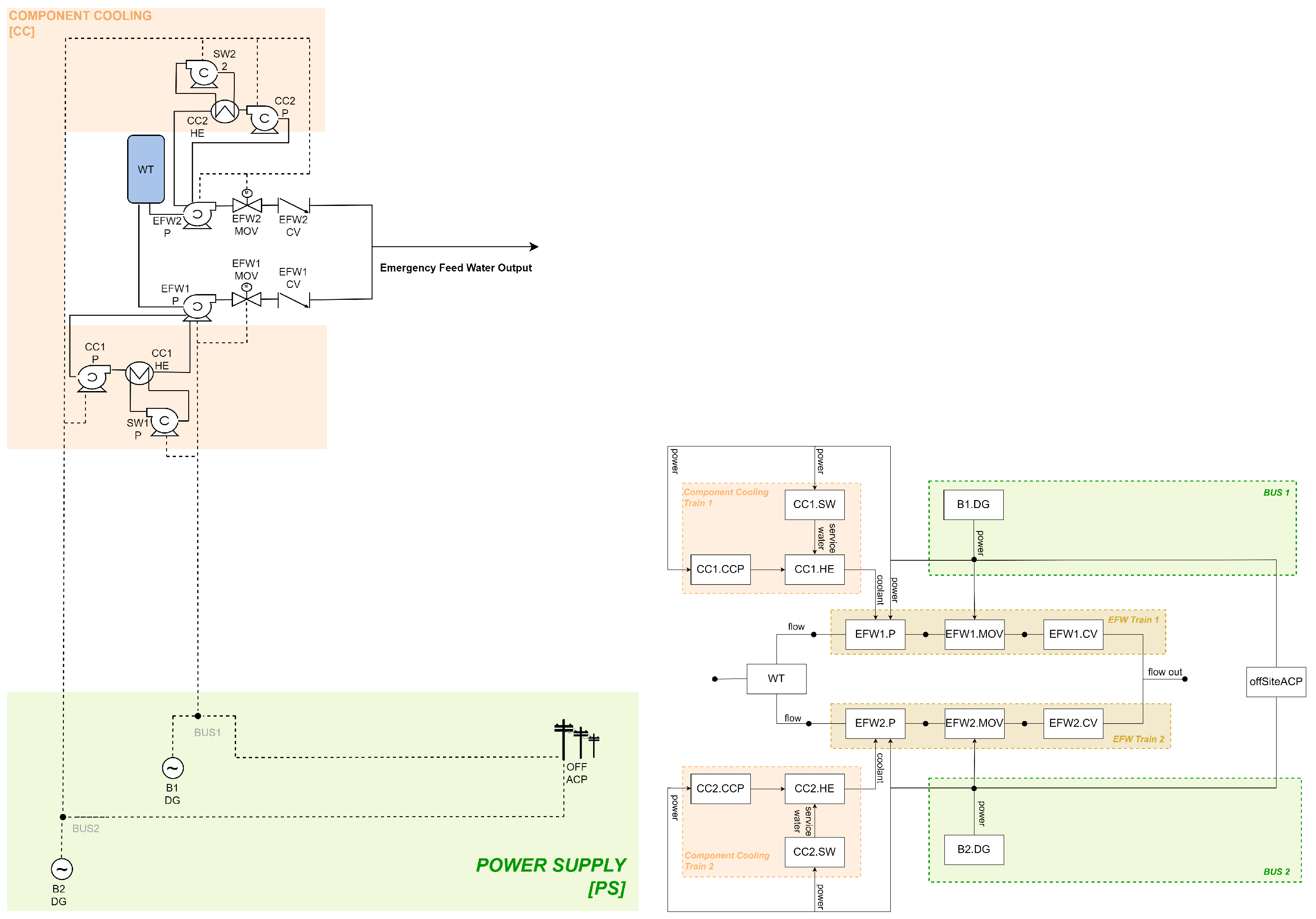
The EFW system provides high-pressure injection if MFW is unavailable. It has two trains (EFW1 and EFW2) drawing from a common water tank WT, each with a pump (EFW1.P and EFW2.P), motorised valve (EFW1.MOV and EFW2.MOV), and check valve (EFW1.CV and EFW2.CV). EFW1 is powered by bus B1 and cooled by CC1; EFW2 by bus B2 and CC2 (Figure 4).

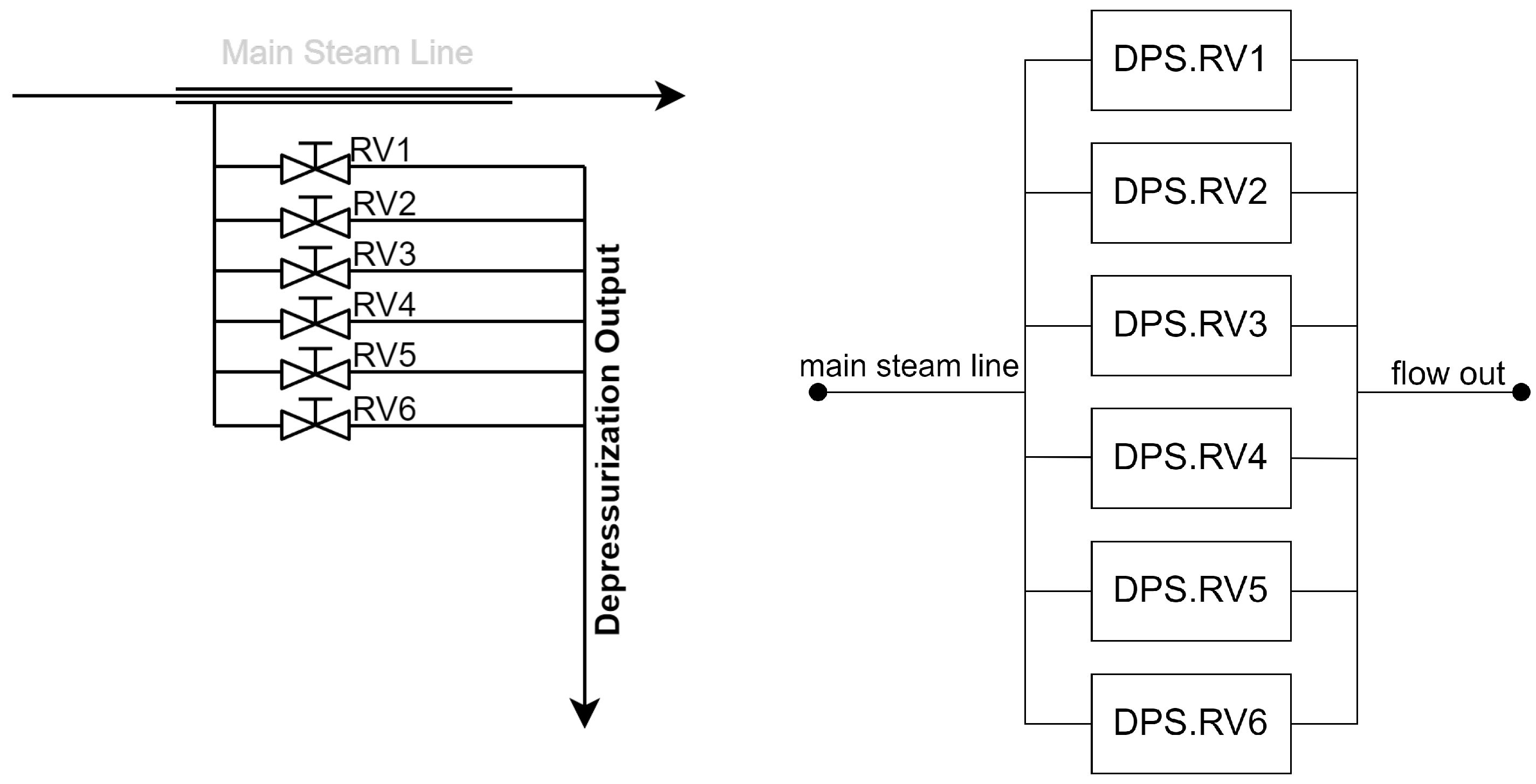
The DPS system reduces vessel pressure to enable low-pressure cooling. As shown in Figure 5, it has six relief valves, of which at least two must open for the function to succeed.

The ECC system (Figure 6) injects low-pressure coolant from the suppression pool CPool through two trains (ECC1 and ECC2), each equipped with a pump (ECC1.P for train 1 and ECC2.P for train 2), motorised valve (ECC1.MOV and ECC2.MOV), and check valve (ECC1.CV and ECC2.CV). Trains ECC1 and ECC2 rely on PS buses B1/B2 and CC trains CC1/CC2, respectively.

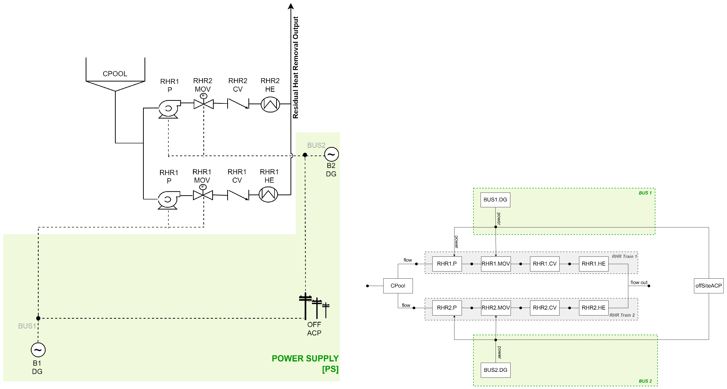
The RHR system removes decay heat during accident recovery. Its two trains RHR1 and RHR2 include a pump (RHR1.P and RHR2.P), motorised valve (RHR1.MOV and RHR2.MOV), check valve (RHR1.CV and RHR2.CV), and heat exchanger (RHR1.HE and RHR2.HE) each. RHR1 is powered by bus B1, RHR2 by B2 (Figure 7).

4.3. System Operation and Asset Management

During normal operation, the MFW, PS, and CC systems are active, while EFW, DPS, ECC, and RHR remain in standby. The backup power sources undergo 48 h maintenance each month on an exclusive basis, meaning that only one generator is taken out of service at a time. The two CC trains alternate 50 h outages every three months, and each emergency train is subject to a 60 h maintenance interval on the same cycle. In all cases, maintenance is carried out exclusively so that at most one train of the same system is unavailable at any given time. In the event of a loss of MFW, the EFW system provides the primary mitigation. Each train is independently capable of restoring reactor conditions to the range required for RHR operation. If both MFW and EFW fail, cooling depends on ECC and RHR acting together, which requires prior depressurisation through DPS. Priority is assigned to trains ECC1 and RHR1: they are activated first and, if failed and restored, return to priority status after repair, placing ECC2 and RHR2 back into standby. The accident sequence is summarised in the event tree of Figure 8.

5. ${\mathbf{D}}^{\mathbf{2}}{\mathbf{T}}^{\mathbf{2}}$ Model Implementation

This section investigates the application of the $D^2{T}^2$ framework to the case study, showing how dependencies are modelled and quantified at three successive levels:

• Basic event level (Section 5.1), illustrated through the EFW subsystem, where dependencies arise mainly from maintenance schedules.
• Intermediate event level (Section 5.2), demonstrated for the ECC subsystem, where alternate standby configurations induce dependencies between component train failures.
• Subsystem level (Section 5.3), where shared support systems (e.g., power, cooling, and condensation pool) introduce cross-subsystem dependencies, which are captured through conditionalisation and integrated into the event tree analysis.

At each level, the $D^2{T}^2$ procedure is contrasted with traditional FT/ET analysis and, where opportune, with fully dynamic models, highlighting how the proposed approach resolves dependencies with accuracy while retaining computational tractability. For clarity and traceability, Appendix A provides a complete list of the failure event labels used in the fault tree models (

Table A2. Basic events included in the FT and BDD models.

Label	Event	Subsystem	Failure Mode
EFW1CV	Failure of EFW1 control valve to open	EFW	On demand
EFW2CV	Failure of EFW2 control valve to open	EFW	On demand
EFW1MOV	Failure of EFW1 motorised valve to open	EFW	On demand
EFW2MOV	Failure of EFW2 motorised valve to open	EFW	On demand
EFW1maint	EFW train 1 unavailable due to maintenance	EFW	Reversible
EFW2maint	EFW train 2 unavailable due to maintenance	EFW	Reversible
EFW1Pop	Failure of EFW1 pump to operate	EFW	Reversible
EFW2Pop	Failure of EFW2 pump to operate	EFW	Reversible
EFW1Pstart	Failure of EFW1 pump to start	EFW	On demand
EFW2Pstart	Failure of EFW2 pump to start	EFW	On demand
WT	Rupture of the water tank	EFW	Irreversible
CPool	Failure of the condensation pool	ECC	Irreversible
ECC1CV	Failure of ECC1 control valve to open	ECC	On demand
ECC2CV	Failure of ECC2 control valve to open	ECC	On demand
ECC1MOV	Failure of ECC1 motorised valve to open	ECC	On demand
ECC2MOV	Failure of ECC2 motorised valve to open	ECC	On demand
ECC1maint	ECC train 1 under maintenance	ECC	Reversible
ECC2maint	ECC train 2 under maintenance	ECC	Reversible
ECC1Pop	Failure of ECC1 pump to operate	ECC	Reversible
ECC2Pop	Failure of ECC2 pump to operate	ECC	Reversible
ECC1Pstart	Failure of ECC1 pump to start	ECC	On demand
ECC2Pstart	Failure of ECC2 pump to start	ECC	On demand
CPool	Failure of the condensation pool	RHR	Irreversible
RHR1CV	Failure of RHR1 control valve to open	RHR	On demand
RHR2CV	Failure of RHR2 control valve to open	RHR	On demand
RHR1HE	Rupture of RHR1 heat exchanger	RHR	Irreversible
RHR2HE	Rupture of RHR2 heat exchanger	RHR	Irreversible
RHR1MOV	Failure of RHR1 motorised valve to open	RHR	On demand
RHR2MOV	Failure of RHR2 motorised valve to open	RHR	On demand
RHR1maint	RHR train 1 under maintenance	RHR	Reversible
RHR2maint	RHR train 2 under maintenance	RHR	Reversible
RHR1Pop	Failure of RHR1 pump to operate	RHR	Reversible
RHR2Pop	Failure of RHR2 pump to operate	RHR	Reversible
RHR1Pstart	Failure of RHR1 pump to start	RHR	On demand
RHR2Pstart	Failure of RHR2 pump to start	RHR	On demand

), together with the list of Petri Net model nodes and their corresponding meaning (

Table A1. Nodes included in the Petri Net models.

Label	Event	Dependency Model
ECC1 SBY	ECC train 1 in standby
ECC2 SBY	ECC train 2 in standby
ECC1(start)	ECC train 1 unavailable due to failure to start
ECC2(start)	ECC train 2 unavailable due to failure to start	ECC trains dependency
ECC1	ECC train 1 unavailable due to failure in operation	(Figure 12)
ECC2	ECC train 2 unavailable due to failure in operation
$\overline{ECC1}$	ECC train 1 operational
$\overline{ECC2}$	ECC train 2 operational
CC1 MNT requested	CC train 1 due for servicing
CC2 MNT requested	CC train 2 due for servicing
CC1 MNT free	CC train 1 not due for servicing
CC2 MNT free	CC train 2 not due for servicing
CC1 MNT	CC train 1 unavailable due to servicing
CC2 MNT	CC train 2 unavailable due to servicing
CC1 MNT ended	CC train 1 servicing completed	CC trains dependency
CC2 MNT ended	CC train 2 servicing completed	(Figure 15)
CC1 (irreversible)	CC train 1 unavailable and not repairable
CC2 (irreversible)	CC train 2 unavailable and not repairable
CC1	CC train 1 failed in operation
CC2	CC train 2 failed in operation
CC1	CC train 1 operational
CC2	CC train 2 operational

). The reliability data adopted in the computations were drawn from the publicly available IAEA databases [27], ensuring consistency with widely accepted international sources.

5.1. Basic Event Level: The EFW System

The EFW subsystem presents two types of dependencies:

• External, due to the reliance on support systems shared with other subsystems;
• Internal, stemming from the maintenance strategy applied to its two trains.

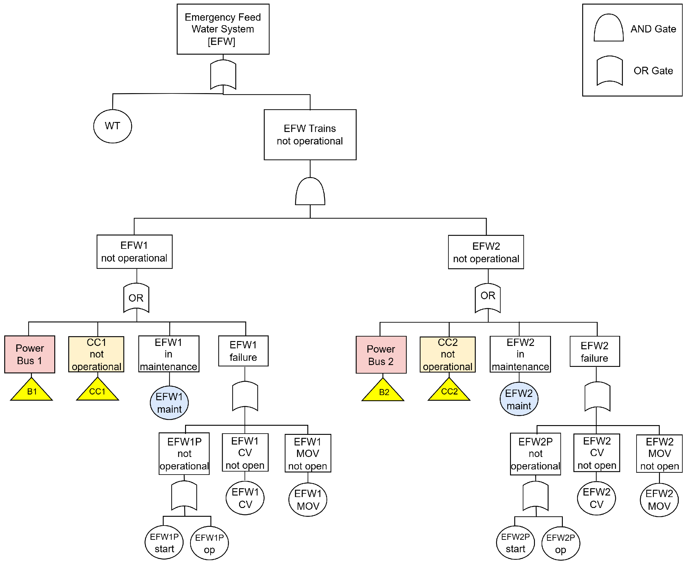
The internal dependency arises from two mechanisms in the EFW maintenance strategy. First, the maintenance events of the two trains (EFW1maint, EFW2maint in Figure 9) are mutually exclusive since only one train can undergo scheduled maintenance at a time. Second, maintenance of one train is suspended whenever the other train is unavailable due to failure. This couples each maintenance event not only to the other maintenance event but also to the corresponding train failure events (EFW1 and EFW2).

In the EFW case, the dependency between train failures and maintenance is negligible because the subsystem is only demanded upon failure of the MFW system, with probability in the order of ${10}^{-5}$. The chance of one train being in maintenance while the other is failed is therefore below ${10}^{-7}$, and can be ignored relative to the overall subsystem failure probability. As a result, the dependency model reduces to the basic maintenance events alone (EFW1maint and EFW2maint).

Since the maintenance schedule in place is deterministic, joint probabilities for the dependency group can be obtained directly without recourse to the dynamic models. Based on a 60 h intervention every three months over four cycles across the mission time of 8760 h, the joint distribution is

$$\begin{array}{cc}\hfill q(EFW1maint,EFW2maint)& =0;\hfill \\ \hfill q(EFW1maint,\overline{EFW2maint})& =q\left(EFW1maint\right)·q(\overline{EFW2maint}|EFW1maint)={\displaystyle \frac{60·4}{8760}}·1=0.0274;\hfill \\ \hfill q(\overline{EFW1maint},EFW2maint)& ={\displaystyle \frac{60·4}{8760}}·1=0.0274;\hfill \\ \hfill q(\overline{EFW1maint},\overline{EFW2maint})& ={\displaystyle \frac{4·(730·3)-120}{8760}}=0.9452;\hfill \end{array}$$

(1)

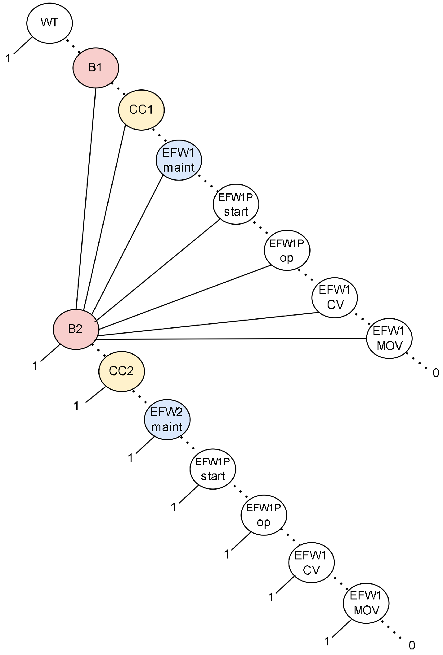
As discussed in Section 3.2, these joint probabilities are then reintroduced into the analysis through the corresponding BDD (Figure 10), which encodes the logic of the FT in Figure 9. The unconditional failure probability of the EFW subsystem is then computed using the $D^2{T}^2$ algorithms [26], taking into account both the FT event data (

Table 1. Basic event data for the EFW FT in Figure 9.

Basic Event	Failure Rate [${\mathbf{h}}^{-1}$]	Repair Time [h]	On Demand Q
EFW1Pstart
EFW2Pstart			$4.80·{10}^{-4}$
EFW1CV
EFW2CV			$8.40·{10}^{-4}$
EFW1MOV
EFW2MOV			$4.10·{10}^{-3}$
EFW1Pop
EFW2Pop	$8.40·{10}^{-6}$	$21.50$
WT	$2.60·{10}^{-8}$

) and the dependency structure of Equation (1).

5.2. Intermediate Event Level: The ECC System

At the intermediate event layer, dependencies arise when the behaviour of whole subsystem sections is linked but cannot be conveniently resolved at the level of their constituent basic events.

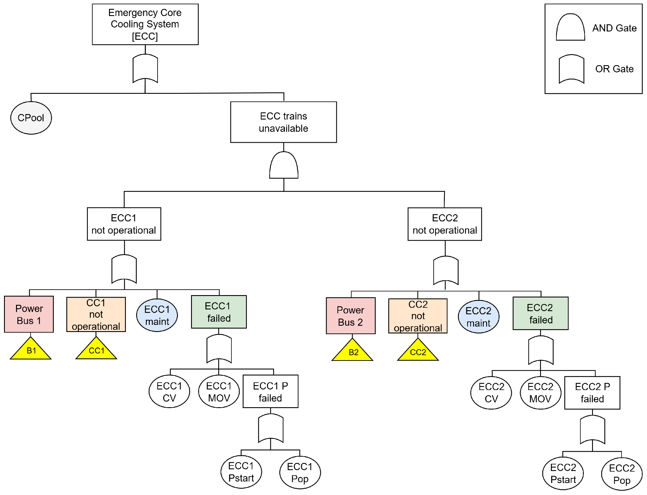
In the ECC system, this occurs due to the mutually exclusive maintenance and standby configuration of the two trains ECC1 and ECC2. The first results in the direct dependency of basic events ECC1maint and ECC2maint and can be treated with the procedure described in Section 5.1 for the EFW system. The second involves instead the intermediate events ECC1failed and ECC2failed in Figure 11, which represent the malfunction of the two subsystem trains: train ECC2 is activated and remains operational only while ECC1 is unavailable, thereby establishing a dependency between their failure events.

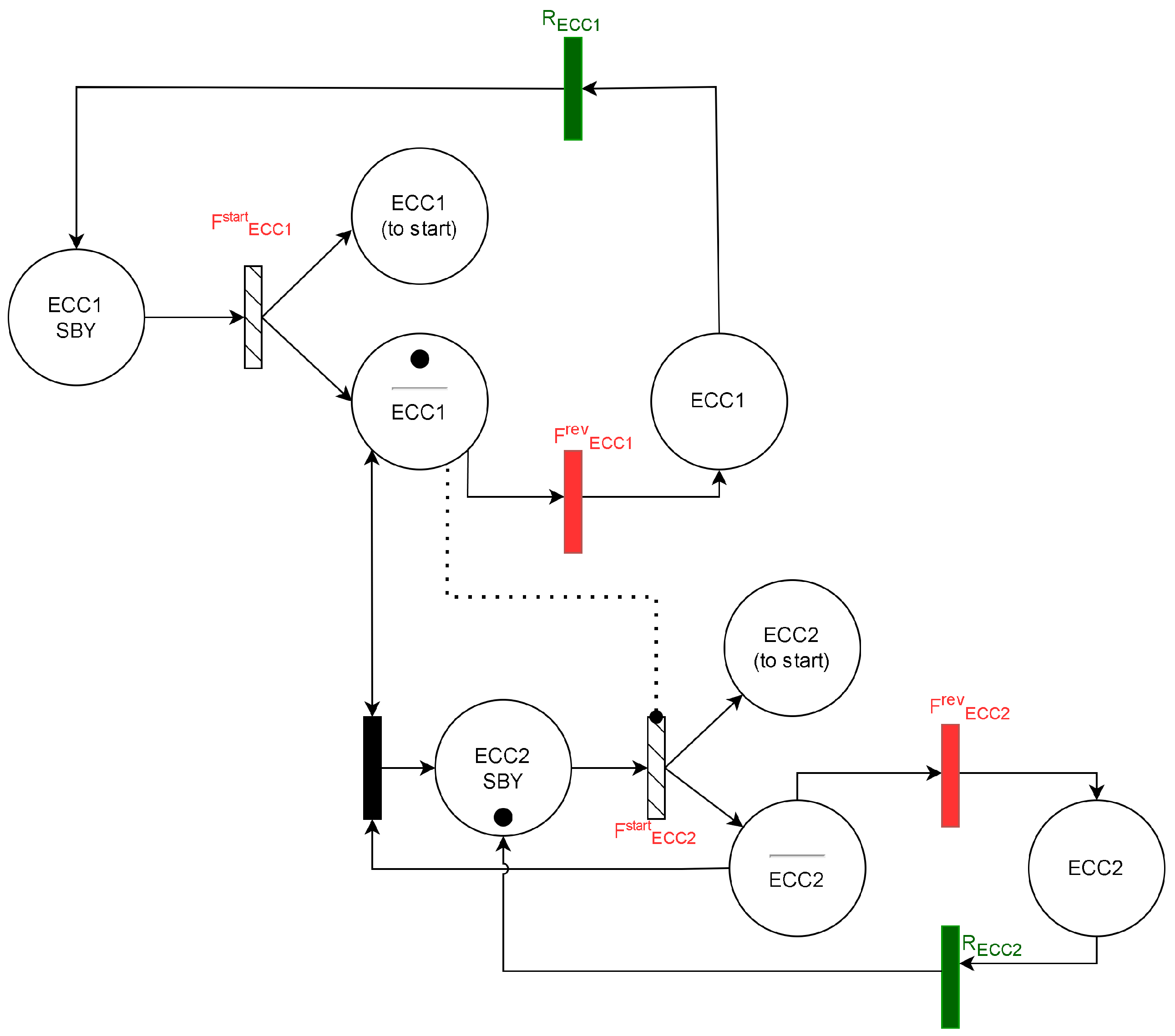
This asset management configuration adopted for the two trains is captured by the PN shown in Figure 12, which mimics the failure mechanisms depicted by the ECC1failed and ECC2failed sub-trees in Figure 11. However, for the dependency model in Figure 11 to be computed, the failure and repair transitions (in red and green in Figure 12, respectively) regulating the changes between the trains states must be known. These are extracted from the analysis of the respective sub-trees, taking into account the nature of the individual failure: the contribution of the basic events embraced by each subtree to the top event metrics must be estimated according to their type.

• Failure to start: Control valves (ECC1CV, ECC2CV), motorised valves (ECC1MOV, ECC2MOV) and pumps (ECC1Pstart, ECC2Pstart) fail on demand, preventing the ECC trains from starting when requested. In the dynamic model of Figure 12, such a failure mechanism is modelled by transitions $F_{ECC1}^{start}$ and $F_{ECC2}^{start}$. These are characterised by point probabilities equal to the sum of the relevant basic events probability associated with components failing on demand.
• Failure in operation: The remaining subtree events ECC1Pop and ECC2Pop refer to the failure of the trains circulation pumps during operation. This failure is reversible and modelled by two sets of transitions in the PN model of Figure 12: one referring to the pumps failure (i.e., $F_{ECC1}^{rev}$ and $F_{ECC2}^{rev}$ in Figure 12) and one associated with their repair times (i.e., $R_{ECC1}$ and $R_{ECC2}$). Details of the related probability distributions are provided in Table 2.

Table 2. Basic event data for the ECC FT in Figure 11.

Basic Event	Failure Rate [${\mathbf{h}}^{-1}$]	Repair Time [h]	On Demand Q
ECC1Pstart
ECC2Pstart			$4.80·{10}^{-4}$
ECC1CV
ECC2CV			$8.40·{10}^{-4}$
ECC1MOV
ECC2MOV			$4.10·{10}^{-3}$
ECC1Pop
ECC2Pop	$8.40·{10}^{-6}$	$21.50$
CPool	$2.60·{10}^{-8}$

Table 2. Basic event data for the ECC FT in Figure 11.

Basic Event	Failure Rate [${\mathbf{h}}^{-1}$]	Repair Time [h]	On Demand Q
ECC1Pstart
ECC2Pstart			$4.80·{10}^{-4}$
ECC1CV
ECC2CV			$8.40·{10}^{-4}$
ECC1MOV
ECC2MOV			$4.10·{10}^{-3}$
ECC1Pop
ECC2Pop	$8.40·{10}^{-6}$	$21.50$
CPool	$2.60·{10}^{-8}$

Solving the PN yields the joint distribution of train states reported in

Table 3. Output of the dynamic model shown in Figure 12.

Trains State	Probability
$\overline{ECC1},\overline{ECC2}$	$8.62·{10}^{-6}$
$\overline{ECC1},ECC2$	$9.95·{10}^{-5}$
$ECC1,\overline{ECC2}$	$2.90·{10}^{-3}$
$ECC1,ECC2$	$9.97·{10}^{-1}$

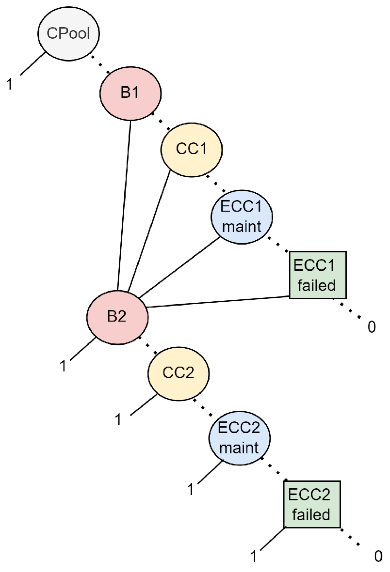
, which characterises the dependency group $\{ECC1failed,ECC2failed\}$. The two subtrees in Figure 11 are then substituted by equivalent basic events associated with this joint distribution. The overall BDD for the ECC system (Figure 13) is evaluated using the $D^2{T}^2$ algorithms [26], which propagate the joint probabilities together with the remaining FT data (Table 2) through the diagram logic.

5.3. Subsystem Level: Shared Resources

In the current case study, shared support infrastructures such as power supply and cooling result in dependencies at the subsystem level. In the $D^2{T}^2$ framework, these are treated by conditionalising subsystem top-event probabilities over the states of the shared subsystems, with joint probabilities then propagated consistently through the Event Tree (ET). This avoids unrealistic independence assumptions while retaining the ET analytical structure.

5.3.1. Conditionalisation over Support Systems

Traditional ET analysis assumes subsystem independence, expressing loss frequencies as the product of subsystem state probabilities and the frequency of the initiating event. For example, the “no loss” scenario in Figure 8 would be calculated as

$$w\left(NoLoss\right)=w\left(MFW\right)q\left(EFW\right)q\left(\overline{DPS}\right)q\left(\overline{ECC}\right)q\left(\overline{RHR}\right)$$

(2)

However, many of the subsystems involved rely on shared support systems, leading to dependencies that extend beyond the boundaries of individual FTs. To take into account this type of dependencies, it is necessary to ‘extract’ the dependency source from the individual FT analysis, instantiating the dependent subsystem FT top probability according to the state of the shared support system. The $D^2{T}^2$ approach achieves this by restricting the associated BDD paths to those consistent with the support systems’ states. Conditional failure probabilities of the dependent subsystems are then obtained for each combination of support system states. For instance, the conditional failure probability of the EFW subsystem given the unavailability of all support systems is

$$q\left(EFW\right|B1,B2,B3,CC1,CC2)=\sum _{i|pat{h}_i\notin \overline{B1},\overline{B2},\overline{B3},\overline{CC1},\overline{CC2}}q\left(pat{h}_i\right)$$

(3)

where $q\left(pat{h}_i\right)$ indicates the probability of any path in Figure 10, which exclude events incompatible with the scenario under consideration (in this case, events referring to the working state of any supply system). Such probability is calculated as net of the associated supply states probability, and then can hence be expressed as

$$q\left(pat{h}_i\right)=\prod _{j|X_j\ne B1,B2,B3,CC1,CC2}q\left(X_j\right)$$

(4)

Applying this procedure to all functional subsystems yields the conditional probability vectors shown in

Table 4. Functional subsystem failure probability vectors.

Support System State	qMFW	qEFW	qDPS	qECC	qRHR
$\overline{B1},\overline{B2},\overline{B3},\overline{CC1},\overline{CC2}$	$8.78·{10}^{-5}$	$5.66·{10}^{-4}$	$9.98·{10}^{-3}$	$9.10·{10}^{-5}$	$1.25·{10}^{-4}$
$\overline{B1},\overline{B2},\overline{B3},\overline{CC1},CC2$	$8.78·{10}^{-5}$	$3.31·{10}^{-2}$	$9.98·{10}^{-3}$	$3.02·{10}^{-2}$	$1.25·{10}^{-4}$
$\overline{B1},\overline{B2},\overline{B3},CC1,\overline{CC2}$	$8.78·{10}^{-5}$	$3.31·{10}^{-2}$	$9.98·{10}^{-3}$	$2.75·{10}^{-2}$	$1.25·{10}^{-4}$
$\overline{B1},\overline{B2},\overline{B3},CC1,CC2$	$8.78·{10}^{-5}$	$1.00·10$	$9.98·{10}^{-3}$	$1.00·10$	$1.25·{10}^{-4}$
$\overline{B1},\overline{B2},B3,\overline{CC1},\overline{CC2}$	$1.00·10$	$5.66·{10}^{-4}$	$9.98·{10}^{-3}$	$9.10·{10}^{-5}$	$1.25·{10}^{-4}$
$\overline{B1},\overline{B2},B3,\overline{CC1},CC2$	$1.00·10$	$3.31·{10}^{-2}$	$9.98·{10}^{-3}$	$3.02·{10}^{-2}$	$1.25·{10}^{-4}$
$\overline{B1},\overline{B2},B3,CC1,\overline{CC2}$	$1.00·10$	$3.31·{10}^{-2}$	$9.98·{10}^{-3}$	$2.75·{10}^{-2}$	$1.25·{10}^{-4}$
$\overline{B1},\overline{B2},B3,CC1,CC2$	$1.00·10$	$1.00·10$	$9.98·{10}^{-3}$	$1.00·10$	$1.25·{10}^{-4}$
$\overline{B1},B2,\overline{B3},\overline{CC1},CC2$	$8.78·{10}^{-5}$	$3.31·{10}^{-2}$	$9.98·{10}^{-3}$	$3.02·{10}^{-2}$	$2.76·{10}^{-2}$
$\overline{B1},B2,\overline{B3},CC1,CC2$	$8.78·{10}^{-5}$	$3.31·{10}^{-2}$	$9.98·{10}^{-3}$	$1.00·10$	$2.76·{10}^{-2}$
$\overline{B1},B2,B3,\overline{CC1},CC2$	$1.00·10$	$3.31·{10}^{-2}$	$9.98·{10}^{-3}$	$3.02·{10}^{-2}$	$2.76·{10}^{-2}$
$\overline{B1},B2,B3,CC1,CC2$	$1.00·10$	$1.00·10$	$9.98·{10}^{-3}$	$1.00·10$	$2.76·{10}^{-2}$
$B1,\overline{B2},\overline{B3},CC1,\overline{CC2}$	$8.78·{10}^{-5}$	$3.31·{10}^{-2}$	$9.98·{10}^{-3}$	$2.75·{10}^{-2}$	$2.75·{10}^{-2}$
$B1,\overline{B2},\overline{B3},CC1,CC2$	$8.78·{10}^{-5}$	$1.00·10$	$9.98·{10}^{-3}$	$1.00·10$	$2.75·{10}^{-2}$
$B1,\overline{B2},B3,CC1,\overline{CC2}$	$1.00·10$	$3.31·{10}^{-2}$	$9.98·{10}^{-3}$	$2.75·{10}^{-2}$	$2.75·{10}^{-2}$
$B1,\overline{B2},B3,CC1,CC2$	$1.00·10$	$1.00·10$	$9.98·{10}^{-3}$	$1.00·10$	$2.75·{10}^{-2}$
$B1,B2,\overline{B3},CC1,CC2$	$8.78·{10}^{-5}$	$1.00·10$	$9.98·{10}^{-3}$	$1.00·10$	$1.00·10$
$B1,B2,B3,CC1,CC2$	$1.00·10$	$1.00·10$	$9.98·{10}^{-3}$	$1.00·10$	$1.00·10$

. These results already provide a further insight in the overall system behaviour compared to conventional FT/ET, where only unconditional probabilities would be used.

5.3.2. ECC and RHR

Beyond support systems, the ECC and RHR subsystems both rely on the condensation pool CPool (see Figure 11 and Figure 14), introducing a further external dependency. Here, subsystem probabilities are conditional not only on the support systems but also on the CPool state. Using the law of total probability, the joint probability of ECC and RHR failure conditional to the working state of the support systems is expressed as

$$\begin{array}{cc}\hfill & q(ECC,RHR|\overline{B1},\overline{B2},\overline{CC1},\overline{CC2})=\hfill \\ \hfill & q\left(ECC\right|\overline{B1},\overline{B2},\overline{CC1},\overline{CC2},CPool)q\left(RHR\right|\overline{B1},\overline{B2},CPool)q\left(CPool\right)\hfill \\ \hfill & +q\left(ECC\right|\overline{B1},\overline{B2},\overline{CC1},\overline{CC2},\overline{CPool})q\left(RHR\right|\overline{B1},\overline{B2},CPool)q\left(\overline{CPool}\right)\hfill \end{array}$$

(5)

Applying the same procedure to all possible combinations of support system states, the joint distributions shown in

Table 5. Conditional joint probability for the ECC and RHR systems.

Support System State	$\mathbf{ECC},\mathbf{RHR}$	$\overline{\mathbf{ECC}},\mathbf{RHR}$	$\mathbf{ECC},\overline{\mathbf{RHR}}$	$\overline{\mathbf{ECC}},\overline{\mathbf{RHR}}$
$\overline{B1},\overline{B2},\overline{B3},\overline{CC1},\overline{CC2}$	$1.12·{10}^{-7}$	$1.00·10$	$9.10·{10}^{-5}$	$1.25·{10}^{-4}$
$\overline{B1},\overline{B2},\overline{B3},\overline{CC1},CC2$	$3.87·{10}^{-6}$	$9.70·{10}^{-1}$	$3.02·{10}^{-2}$	$1.21·{10}^{-4}$
$\overline{B1},\overline{B2},\overline{B3},CC1,\overline{CC2}$	$3.53·{10}^{-6}$	$9.72·{10}^{-1}$	$2.75·{10}^{-2}$	$1.21·{10}^{-4}$
$\overline{B1},\overline{B2},\overline{B3},CC1,CC2$	$1.25·{10}^{-4}$	0	$1.00·10$	0
$\overline{B1},\overline{B2},B3,\overline{CC1},\overline{CC2}$	$1.12·{10}^{-7}$	$1.00·10$	$9.09·{10}^{-5}$	$1.25·{10}^{-4}$
$\overline{B1},\overline{B2},B3,\overline{CC1},CC2$	$3.87·{10}^{-6}$	$9.70·{10}^{-1}$	$3.02·{10}^{-2}$	$1.21·{10}^{-4}$
$\overline{B1},\overline{B2},B3,CC1,\overline{CC2}$	$3.53·{10}^{-6}$	$9.72·{10}^{-1}$	$2.75·{10}^{-2}$	$1.21·{10}^{-4}$
$\overline{B1},\overline{B2},B3,CC1,CC2$	$1.25·{10}^{-4}$	0	$1.00·10$	0
$\overline{B1},B2,\overline{B3},\overline{CC1},CC2$	$8.36·{10}^{-4}$	$9.43·{10}^{-1}$	$2.94·{10}^{-2}$	$2.68·{10}^{-2}$
$\overline{B1},B2,\overline{B3},CC1,CC2$	$8.36·{10}^{-4}$	$9.43·{10}^{-1}$	$2.94·{10}^{-2}$	$2.68·{10}^{-2}$
$\overline{B1},B2,B3,\overline{CC1},CC2$	$8.36·{10}^{-4}$	$9.43·{10}^{-1}$	$2.94·{10}^{-2}$	$2.68·{10}^{-2}$
$\overline{B1},B2,B3,CC1,CC2$	$2.76·{10}^{-2}$	0	$9.72·{10}^{-1}$	0
$B1,\overline{B2},\overline{B3},CC1,\overline{CC2}$	$7.57·{10}^{-4}$	$9.46·{10}^{-1}$	$2.67·{10}^{-2}$	$2.68·{10}^{-2}$
$B1,\overline{B2},\overline{B3},CC1,CC2$	$2.75·{10}^{-2}$	0	$9.72·{10}^{-1}$	0
$B1,\overline{B2},B3,CC1,\overline{CC2}$	$7.57·{10}^{-4}$	$9.46·{10}^{-1}$	$2.67·{10}^{-2}$	$2.68·{10}^{-2}$
$B1,\overline{B2},B3,CC1,CC2$	$2.75·{10}^{-2}$	0	$9.72·{10}^{-1}$	0
$B1,B2,\overline{B3},CC1,CC2$	$1.00·10$	0	0	0
$B1,B2,B3,CC1,CC2$	$1.00·10$	0	0	0

are obtained. These are then marginalised to yield the conditional subsystem vectors used in Table 4: these are complemental to the vector of support system states joint probabilities, which remains to be calculated.

5.3.3. CC Trains and Power Buses

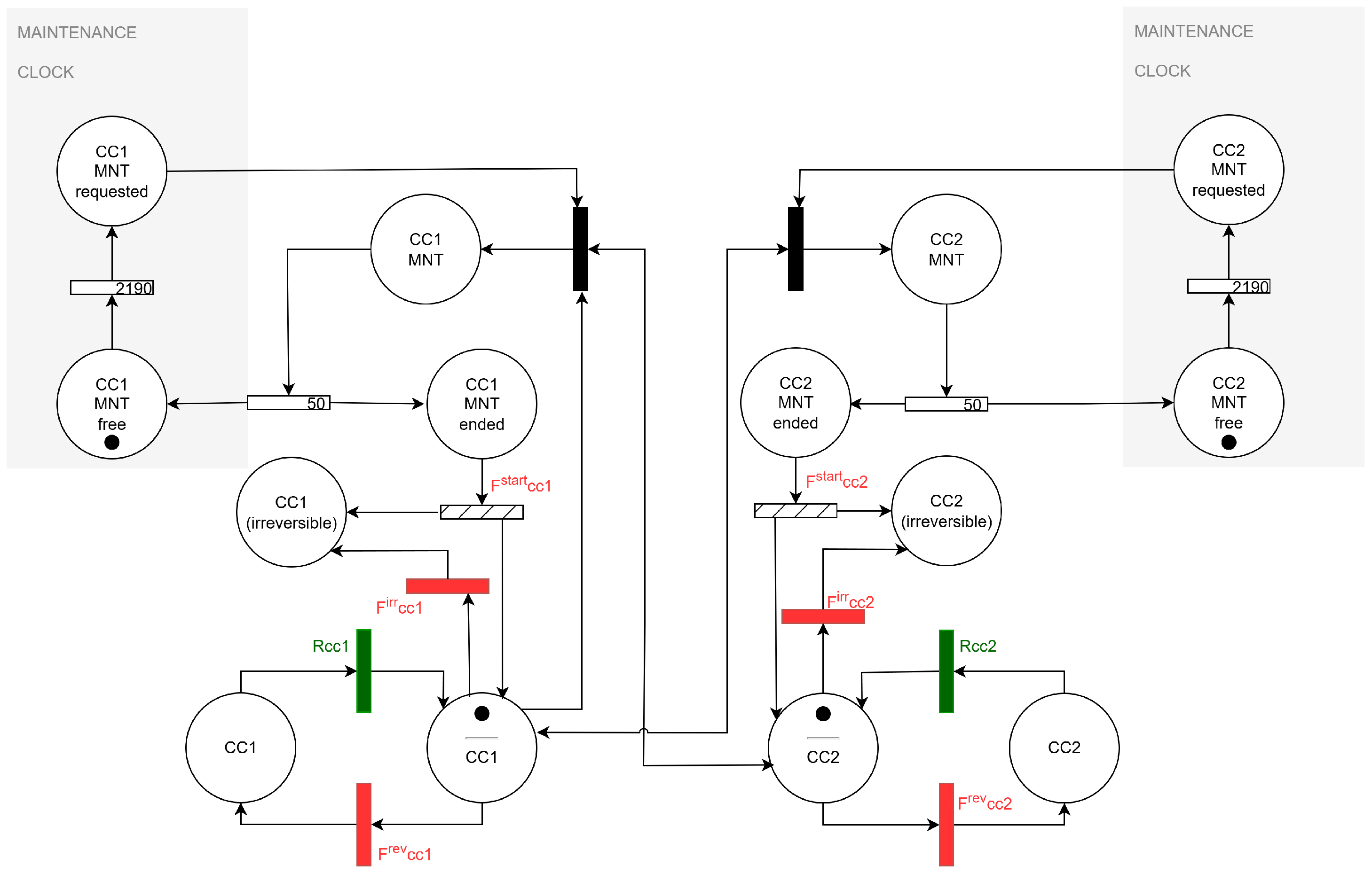
The modelling of the component cooling trains CC1 and CC2 illustrates how different dependency assumptions can be captured. Both trains are subject to mutually exclusive maintenance, but in practice the maintenance of one train may be suspended if the other is unavailable (due to mechanical failure or power loss). Two cases were analysed: Case A assumes dependencies are limited to maintenance exclusivity, while Case B extends this to include interruptions from train failures. Case B requires the use of the dynamic model in Figure 15, whereas Case A remains analytically tractable with two dependency groups.

Table 6. Comparison of joint failure probabilities for the CC subsystem under different modelling assumptions.

Event	FT	${\mathit{D}}^2{\mathit{T}}^2$	${\mathit{D}}^2{\mathit{T}}^2$	Dynamic
		Case A	Case B
$CC1,CC2$	$5.53·{10}^{-3}$	$4.04·{10}^{-3}$	$3.78·{10}^{-4}$	$3.30·{10}^{-4}$
$CC1,\overline{CC2}$	$4.11·{10}^{-2}$	$4.16·{10}^{-2}$	$2.50·{10}^{-2}$	$2.49·{10}^{-2}$

compares the resulting joint probabilities of the support CC trains with those obtained using traditional FT and a fully dynamic benchmark.

5.4. Integration into ET Analysis

The conditional reliability metrics listed in Table 4 and Table 5 must be consistently integrated within the ET framework. The $D^2{T}^2$ procedure achieves this by shifting the computation to a vectorial format: conditional probability vectors are used in place of point values, while the overall ET logic remains unchanged. For example, the frequency associated with the total loss of cooling, as modelled in Figure 8, can be expressed as

$$\begin{array}{cc}\hfill \mathbf{W}\left(\mathbf{Total}\right)& =\mathbf{w}\left(MFW\right|\mathbf{SS})\odot \mathbf{q}(EFW\left|\mathbf{SS}\right)\odot \mathbf{q}\left(DPS\right|\mathbf{SS})\odot \mathbf{Q}(\mathbf{SS})\hfill \\ \hfill & +\mathbf{f}\left(MFW\right|\mathbf{SS})\odot \mathbf{q}\left(EFW\right|\mathbf{SS})\odot \mathbf{q}\left(\overline{DPS}\right)\odot \mathbf{q}\left(ECC\right|\mathbf{SS})\odot \mathbf{Q}\left(\mathbf{SS}\right)\hfill \end{array}$$

(6)

where ⊙ denotes element-wise multiplication, $\mathbf{q}\left(EFW\right|\mathbf{SS})$, $\mathbf{q}\left(DPS\right|\mathbf{SS})$, and $\mathbf{q}\left(ECC\right|\mathbf{SS})$ are the conditional vectors in Table 4, and $\mathbf{Q}\left(\mathbf{SS}\right)$ is the unconditional support-system probability vector in

Table 7. Probability of the joint states of the CC trains and buses B1 and B2.

Support Systems State	FT	${\mathit{D}}^2{\mathit{T}}^2$	${\mathit{D}}^2{\mathit{T}}^2$	Dynamic
		Case A	Case B
$\overline{B1},\overline{B2},\overline{B3},\overline{C1},\overline{C2}$	$9.16·{10}^{-1}$	$9.15·{10}^{-1}$	$9.50·{10}^{-1}$	$9.50·{10}^{-1}$
$\overline{B1},\overline{B2},\overline{B3},\overline{CC1},CC2$	$4.11·{10}^{-2}$	$4.16·{10}^{-2}$	$2.50·{10}^{-2}$	$2.49·{10}^{-2}$
$\overline{B1},\overline{B2},\overline{B3},CC1,\overline{CC2}$	$4.11·{10}^{-2}$	$4.16·{10}^{-2}$	$2.50·{10}^{-2}$	$2.49·{10}^{-2}$
$\overline{B1},\overline{B2},\overline{B3},CC1,CC2$	$1.84·{10}^{-3}$	$1.35·{10}^{-3}$	$1.26·{10}^{-4}$	$1.10·{10}^{-4}$
$\overline{B1},\overline{B2},B3,\overline{CC1},\overline{CC2}$	$2.45·{10}^{-5}$	$1.52·{10}^{-6}$	$1.57·{10}^{-6}$	$2.45·{10}^{-6}$
$\overline{B1},\overline{B2},B3,\overline{CC1},CC2$	$1.10·{10}^{-6}$	$6.90·{10}^{-8}$	$4.14·{10}^{-8}$	$4.95·{10}^{-8}$
$\overline{B1},\overline{B2},B3,CC1,\overline{CC2}$	$1.10·{10}^{-6}$	$6.90·{10}^{-8}$	$4.14·{10}^{-8}$	$5.16·{10}^{-8}$
$\overline{B1},\overline{B2},B3,CC1,CC2$	$4.93·{10}^{-8}$	$2.23·{10}^{-9}$	$2.08·{10}^{-10}$	$3.42·{10}^{-10}$
$\overline{B1},B2,\overline{B3},\overline{CC1},CC2$	$2.63·{10}^{-6}$	$2.12·{10}^{-6}$	$2.11·{10}^{-6}$	$2.52·{10}^{-6}$
$\overline{B1},B2,\overline{B3},CC1,CC2$	$1.18·{10}^{-7}$	$9.53·{10}^{-8}$	$5.54·{10}^{-8}$	$4.08·{10}^{-8}$
$\overline{B1},B2,B3,\overline{CC1},CC2$	$2.14·{10}^{-6}$	$2.34·{10}^{-8}$	$2.33·{10}^{-8}$	$6.82·{10}^{-8}$
$\overline{B1},B2,B3,C1,C2$	$9.59·{10}^{-8}$	$1.05·{10}^{-9}$	$6.11·{10}^{-10}$	$1.71·{10}^{-9}$
$B1,\overline{B2},\overline{B3},CC1,\overline{CC2}$	$2.63·{10}^{-6}$	$2.18·{10}^{-6}$	$2.16·{10}^{-6}$	$2.53·{10}^{-6}$
$B1,\overline{B2},\overline{B3},CC1,CC2$	$1.18·{10}^{-7}$	$9.78·{10}^{-8}$	$5.68·{10}^{-8}$	$4.13·{10}^{-8}$
$B1,\overline{B2},B3,CC1,\overline{CC2}$	$2.14·{10}^{-6}$	$2.35·{10}^{-8}$	$2.34·{10}^{-8}$	$6.99·{10}^{-8}$
$B1,\overline{B2},B3,CC1,CC2$	$9.59·{10}^{-8}$	$1.06·{10}^{-9}$	$6.14·{10}^{-10}$	$1.29·{10}^{-9}$
$B1,B2,\overline{B3},CC1,CC2$	$2.29·{10}^{-7}$	$4.58·{10}^{-8}$	$4.47·{10}^{-8}$	$6.77·{10}^{-8}$
$B1,B2,B3,CC1,CC2$	$1.87·{10}^{-7}$	$3.52·{10}^{-10}$	$3.44·{10}^{-10}$	$1.80·{10}^{-9}$

.

Similarly, the no loss frequency is

$$\begin{array}{cc}\hfill \mathbf{W}\left(\mathbf{None}\right)& =\mathbf{f}\left(MFW\right|\mathbf{SS})\odot \mathbf{q}\left(\overline{EFW}\right|\mathbf{SS})\odot \mathbf{q}\left(\overline{RHR}\right|\mathbf{SS})\odot \mathbf{Q}\left(\mathbf{SS}\right)\hfill \\ \hfill & +\mathbf{f}\left(MFW\right|\mathbf{SS})\odot \mathbf{q}\left(EFW\right|\mathbf{SS})\odot \mathbf{q}\left(\overline{DPS}\right)\odot \mathbf{q}(\overline{ECC},\overline{RHR}|\mathbf{SS})\odot \mathbf{Q}\left(\mathbf{SS}\right)\hfill \end{array}$$

(7)

where the joint probability vector in Table 5 is used for ECC and RHR to reflect their common reliance on the condensation pool.

Finally, partial loss frequencies are obtained as

$$\begin{array}{cc}\hfill \mathbf{F}\left(\mathbf{Partial}\right)& =\mathbf{f}\left(MFW\right|\mathbf{SS})\odot \mathbf{q}\left(\overline{EFW}\right|\mathbf{SS})\odot \mathbf{q}\left(RHR\right|\mathbf{SS})\odot \mathbf{Q}\left(\mathbf{SS}\right)\hfill \\ \hfill & +\mathbf{f}\left(MFW\right|\mathbf{SS})\odot \mathbf{q}\left(EFW\right|\mathbf{SS})\odot \mathbf{q}\left(\overline{DPS}\right)\odot \mathbf{q}(\overline{ECC},RHR|\mathbf{SS})\odot \mathbf{Q}\left(\mathbf{SS}\right)\hfill \end{array}$$

(8)

This vector-based formulation ensures that dependencies among subsystems and support resources are propagated throughout the ET without altering its logic, preserving interpretability while extending analytical fidelity.

6. Results

The application of the $D^2{T}^2$ framework to the case study demonstrates its ability to refine reliability predictions across multiple modelling layers, correcting distortions introduced by the independence assumption in traditional FT/ET analysis.

For the EFW system, where dependencies arise from mutually exclusive maintenance scheduling, the $D^2{T}^2$ procedure yields a top event probability of $2.3·{10}^{-3}$—over 1.5 times lower than the $3.7·{10}^{-3}$ estimate from conventional FT analysis. This illustrates how even basic-event level dependency modelling can significantly improve accuracy.

A more substantial correction is observed for the ECC subsystem, where standby logic introduces operational dependencies between ECC1 and ECC2. The $D^2{T}^2$ analysis produces an unconditional top event probability of $1.65·{10}^{-3}$, compared to $5.53·{10}^{-3}$ under the independence assumption. This shows how $D^2{T}^2$ can capture dynamic features at higher system levels—such as train standby effects—without requiring full decomposition into basic events. By keeping supporting dynamic models small and intuitive, the approach simplifies model construction and reduces the risk of state–space explosion.

The analysis of the support systems further illustrates the flexibility of $D^2{T}^2$ and its positioning between traditional FT/ET and fully dynamic models. For the CC subsystem, results vary depending on the modelling assumptions. Under the more detailed Case B configuration, $D^2{T}^2$ closely matches the dynamic benchmark with minimal error (${10}^{-4}$–${10}^{-10}$), while Case A offers intermediate accuracy at lower modelling cost. Table 6 compares joint failure probabilities for representative states, showing that traditional FT analysis consistently overestimates failure likelihoods, whereas Case B achieves near-perfect agreement.

A broader comparison across the full spectrum of support system states (Table 7) confirms these trends. FT analysis tends to produce conservative estimates, while $D^2{T}^2$ narrows the gap toward dynamic benchmarks. Case B consistently delivers high accuracy, while Case A provides a practical compromise between fidelity and effort.

When subsystem results are integrated at the ET level, the influence of dependency treatment becomes even more apparent. Adopting the joint probability values for support systems (Table 7, Case B) together with functional system conditional probabilities (Table 4), the overall unconditional loss frequencies are obtained as reported in

Table 8. Loss frequencies estimated by FT and $D^2{T}^2$.

Loss Magnitude	Frequency [FT]	Frequency [${\mathit{D}}^2{\mathit{T}}^2$]
None	$1.87·{10}^{-6}$  ${\mathrm{h}}^{-1}$	$3.57·{10}^{-6}$  ${\mathrm{h}}^{-1}$
Partial	$4.84·{10}^{-9}$  ${\mathrm{h}}^{-1}$	$1.73·{10}^{-9}$  ${\mathrm{h}}^{-1}$
Total	$1.07·{10}^{-10}$  ${\mathrm{h}}^{-1}$	$2.32·{10}^{-9}$  ${\mathrm{h}}^{-1}$

.

Overall, the two approaches appear superficially consistent for partial or no-loss outcomes, with results within the same order of magnitude. However, the apparent agreement masks a compensation of errors: FT analysis tends to overestimate subsystem unavailability by neglecting realistic standby behaviour and maintenance strategies, while simultaneously underestimating loss frequencies at the ET level by ignoring dependencies among subsystems. The comparison highlights that while FT/ET may sometimes yield results numerically close to more refined methods, such convergence is incidental and provides no guarantee of conservatism or accuracy. The most significant discrepancy arises for total loss of cooling, where $D^2{T}^2$ predicts a frequency more than 20 times higher than FT analysis. This reflects its ability to account for shared dependencies and resource constraints that traditional methods overlook.

7. Discussion

The results demonstrate that $D^2{T}^2$ offers a more nuanced and accurate representation of system behaviour across multiple modelling layers. By explicitly incorporating dependencies—whether at the basic-event, intermediate, or subsystem level—the methodology corrects distortions introduced by traditional FT/ET assumptions and improves the credibility of reliability estimates.

A key strength of $D^2{T}^2$ lies in its flexibility. The analyst can tune model fidelity based on available data, system complexity, and computational constraints. The comparison between Case A and Case B in the CC subsystem illustrates this trade-off: Case B achieves near-perfect alignment with dynamic benchmarks, while Case A provides reasonable accuracy with reduced modelling effort. This adaptability makes $D^2{T}^2$ particularly valuable in practical applications, where time and resources may be limited.

Importantly, $D^2{T}^2$ retains the structure and interpretability of FT/ET models, enabling reuse of existing PSA frameworks and compatibility with established analytical tools. This lowers the barrier to adoption and supports integration into current safety assessment workflows.

However, the approach is not without limitations. The accuracy of results depends on the quality of the dependency models and the assumptions made during their construction. Careful judgment is required in selecting which dependencies to include and how to represent them. Nevertheless, this effort is not a fixed burden. Thanks to its flexibility, $D^2{T}^2$ allows the analyst to tune the level of detail to the system under study. Dependencies can be introduced selectively, focusing only on behaviours or configurations that are relevant to overall system performance. In this sense, the strength of the approach lies not only in its ability to improve accuracy but in its capacity to replace implicit assumptions—such as full independence in conventional FT/ET—with explicit and informed modelling choices that promote a deeper understanding of the system.

This advantage extends beyond traditional FT/ET methods to more recent extensions, which, while more expressive, often rely on predefined templates or require substantial modelling effort. In contrast, $D^2{T}^2$ avoids structural constraints and allows the analyst to interrogate any part of the system with virtually no limitations on dependency type or location. At the same time, the reuse of existing FT/ET models and the compact nature of supporting submodels help keep the analysis intuitive and accessible. This reduces the need to learn new modelling languages or engage with overly complex formalisms, preserving clarity and interpretability throughout the process. As a result, analysts can focus on understanding the system itself, rather than navigating technical constraints, enabling more meaningful and targeted modelling.

Future work could focus on supporting this process further with automated tools dedicated to model generation and validation, further reducing the analyst’s burden and promoting model standardisation.

Ultimately, the strength of $D^2{T}^2$ lies not only in its ability to improve analytical accuracy, but in its capacity to make modelling assumptions explicit, transparent, and adaptable to the needs of the system under study. Rather than occupying a fixed position between traditional PSA and fully dynamic modelling, $D^2{T}^2$ operates along a continuum. Depending on the nature of the system and the assumptions adopted, it can reproduce the simplicity of FT/ET, match the fidelity of dynamic models, or settle anywhere in between. This flexibility allows analysts to tailor the modelling effort to the problem at hand, introducing dependencies only where they are meaningful, and keeping supporting models compact and intuitive.

Overall, $D^2{T}^2$ offers a scalable and transparent framework that combines the interpretability of traditional PSA with the ability to model complex interdependencies, making it well-suited for safety-critical applications.

8. Conclusions

This study applied the Dynamic and Dependent Tree Theory ($D^2{T}^2$) to a loss of main feed water accident in a boiling water reactor, demonstrating its ability to capture dependencies across multiple modelling layers while preserving the transparency of Fault Tree and Event Tree analysis. Results showed that $D^2{T}^2$ improves the accuracy of reliability estimates compared with traditional PSA, aligning closely with dynamic benchmarks, while remaining computationally tractable. Its flexibility allows analysts to tune the level of fidelity to the system and data at hand, avoiding both the rigidity of template-based approaches and the complexity of full dynamic models.

Beyond improved accuracy, the main contribution of $D^2{T}^2$ lies in making modelling assumptions explicit and transparent, enabling analysts to interrogate the system without structural restrictions. By reusing existing FT/ET models, it lowers barriers to adoption and supports integration into established PSA workflows. There is also potential to further reduce effort and promote standardisation through greater automation of dependency modelling.

Overall, $D^2{T}^2$ provides a practical and transparent methodology that combines the interpretability of traditional PSA with the ability to capture complex dependencies, positioning it as a scalable alternative to fully dynamic reliability approaches for safety-critical applications.

References

- Ruijters, E.; Stoelinga, M. Fault tree analysis: A survey of the state-of-the-art in modeling, analysis and tools. Comput. Sci. Rev. 2015, 15, 29–62. [Google Scholar] [CrossRef]
- Rauzy, A. New algorithms for fault trees analysis. Reliab. Eng. Syst. Saf. 1993, 40, 203–211. [Google Scholar] [CrossRef]
- Čepin, M. Event tree analysis. In Assessment of Power System Reliability: Methods and Applications; Springer: London, UK, 2011; pp. 89–99. [Google Scholar]
- Andrews, J.; Tolo, S. Dynamic and dependent tree theory (D2T2): A framework for the analysis of fault trees with dependent basic events. Reliab. Eng. Syst. Saf. 2023, 230, 108959. [Google Scholar] [CrossRef]
- Tolo, S.; Andrews, J. Modelling complexity in system safety: Generalizing the D2T2 methodology. arXiv 2025, arXiv:2510.17351. [Google Scholar] [CrossRef]
- Čepin, M.; Mavko, B. A dynamic fault tree. Reliab. Eng. Syst. Saf. 2002, 75, 83–91. [Google Scholar] [CrossRef]
- Zhu, C.; Zhang, T. A review on the realization methods of dynamic fault tree. Qual. Reliab. Eng. Int. 2022, 38, 3233–3251. [Google Scholar] [CrossRef]
- Aslansefat, K.; Kabir, S.; Gheraibia, Y.; Papadopoulos, Y. Dynamic fault tree analysis: State-of-the-art in modeling, analysis, and tools. In Reliability Management and Engineering; CRC Press: Boca Raton, FL, USA, 2020; pp. 73–112. [Google Scholar]
- Palshikar, G.K. Temporal fault trees. Inf. Softw. Technol. 2002, 44, 137–150. [Google Scholar] [CrossRef]
- Kabir, S.; Geok, T.K.; Kumar, M.; Yazdi, M.; Hossain, F. A method for temporal fault tree analysis using intuitionistic fuzzy set and expert elicitation. IEEE Access 2019, 8, 980–996. [Google Scholar] [CrossRef]
- Bouissou, M.; Bon, J.L. A new formalism that combines advantages of fault-trees and Markov models: Boolean logic driven Markov processes. Reliab. Eng. Syst. Saf. 2003, 82, 149–163. [Google Scholar] [CrossRef]
- Piriou, P.Y.; Faure, J.M.; Lesage, J.J. Generalized Boolean logic Driven Markov Processes: A powerful modeling framework for Model-Based Safety Analysis of dynamic repairable and reconfigurable systems. Reliab. Eng. Syst. Saf. 2017, 163, 57–68. [Google Scholar] [CrossRef]
- Reisig, W. Petri Nets: An Introduction; Springer Science & Business Media: Berlin/Heidelberg, Germany, 2012; Volume 4. [Google Scholar]
- Kumari, R.; Naick, B.K.; Ghosh, D. Reliability assessment of distribution system using Petri net for enhancement of situational awareness. Electr. Power Syst. Res. 2023, 224, 109739. [Google Scholar] [CrossRef]
- Tyagi, R.; Saini, P.K. A Comparative Review of Petri Nets and Analytical Techniques for Evaluating RAM in Complex Industrial Systems. Int. J. Reliab. Risk Saf. Theory Appl. 2025, 8, 114–121. [Google Scholar]
- Gagniuc, P.A. Markov Chains: From Theory to Implementation and Experimentation; John Wiley & Sons: Hoboken, NJ, USA, 2017. [Google Scholar]
- Acosta, C.; Siu, N. Dynamic event trees in accident sequence analysis: Application to steam generator tube rupture. Reliab. Eng. Syst. Saf. 1993, 41, 135–154. [Google Scholar] [CrossRef]
- Alfonsi, A.; Rabiti, C.; Mandelli, D.; Cogliati, J.; Kinoshita, R.A.; Naviglio, A. Dynamic Event Tree Analysis Through RAVEN. In Proceedings of the International Topical Meeting on Probabilistic Safety Assessment and Analysis 2013, PSA 2013, Columbia, SC, USA, 22–26 September 2013. [Google Scholar]
- Glingler, T.; Alfonsi, A.; Mandelli, D.; Giannetti, F.; Caruso, G.; D’Onorio, M. Dynamic event tree analysis of a severe accident sequence in a boiling water reactor experiencing a cyberattack scenario. Ann. Nucl. Energy 2023, 192, 109994. [Google Scholar] [CrossRef]
- Gaurav, K.; Kumar, V.; Singh, B.K. Dependability Analysis of a System Using State-Space Modeling Techniques: A Systematic Review. IEEE Trans. Reliab. 2023, 72, 1340–1354. [Google Scholar] [CrossRef]
- Chiacchio, F.; D’Urso, D.; Compagno, L.; Pennisi, M.; Pappalardo, F.; Manno, G. SHyFTA, a Stochastic Hybrid Fault Tree Automaton for the modelling and simulation of dynamic reliability problems. Expert Syst. Appl. 2016, 47, 42–57. [Google Scholar] [CrossRef]
- Zheng, Y.; Zhang, Y. Reliability analysis for system with dependent components based on survival signature and copula theory. Reliab. Eng. Syst. Saf. 2023, 238, 109402. [Google Scholar] [CrossRef]
- Zheng, X.; Tamaki, H.; Sugiyama, T.; Maruyama, Y. Dynamic probabilistic risk assessment of nuclear power plants using multi-fidelity simulations. Reliab. Eng. Syst. Saf. 2022, 223, 108503. [Google Scholar] [CrossRef]
- Maidana, R.G.; Parhizkar, T.; Gomola, A.; Utne, I.B.; Mosleh, A. Supervised dynamic probabilistic risk assessment: Review and comparison of methods. Reliab. Eng. Syst. Saf. 2023, 230, 108889. [Google Scholar] [CrossRef]
- Tolo, S.; Andrews, J. An integrated modelling framework for complex systems safety analysis. Qual. Reliab. Eng. Int. 2022, 38, 4330–4350. [Google Scholar] [CrossRef]
- Tolo, S.; Andrews, J. Fault Tree analysis including component dependencies. IEEE Trans. Reliab. 2023, 73, 413–421. [Google Scholar] [CrossRef]
- International Atomic Energy Agency. Component Reliability Data for Use in Probabilistic Safety Assessment; Number 478 in TECDOC Series; IAEA: Vienna, Austria, 1988. [Google Scholar]