Abstract
Considering the effects of complex correlations between variables and uncertainty of degradation processes in multivariate degradation systems, a system reliability assessment method that integrated Chatterjee correlation coefficient and stochastic process theory is proposed. First, due to temporal uncertainty and measurement error in the univariate degradation process, a general Wiener-process-based state space model is constructed to determine the marginal distributions. Secondly, the nonlinear and asymmetric correlation between variables is analyzed by the nonparametric Chatterjee correlation coefficient. The multivariate joint degradation model is constructed by combining the Vine copula technique. The copula structure selection is optimized based on the goodness-of-fit criterion for modeling the degradation dependency network. In order to verify the validity of the method, comparative experiments based on the C-MAPSS aero-engine degradation dataset are conducted. Compared with the independent model ignoring the correlation of the variables, Vine copula with Chatterjee coefficient shows the rationality of the system reliability assessment. The system reliability curve lies between the cases of complete independence and complete dependence of variables. Compared to the traditional Vine copula model with Kendall coefficient, the method in this paper shows a significant improvement in asymmetric correlation characterization, with a Vuong test value of 6.37. The assessment method given in this paper provided an improved paradigm for reliability assessments of complex systems.
1. Introduction
1.1. Motivation
Prognostics and Health Management (PHM) integrates advanced technologies, including sensors, data analytics, artificial intelligence, and machine learning, to enable real-time system monitoring, fault prediction, and maintenance management. For safety-critical engineering systems, such as aero-engines, turbopumps, and wind turbines, PHM is a core process for ensuring long-term safe and stable operation, optimizing maintenance strategies, and achieving cost control. In the era of big data and Industry 4.0, with the rapid development of sensor technology, modern industrial systems are able to realize fine monitoring of degradation processes through multi-dimensional performance characteristics (PCs), such as vibration spectra, temperature gradients, pressure fluctuations [1]. This trend provides a richer database for system reliability assessment and remaining useful life (RUL) prediction, but also brings new challenges [2].
On one hand, the complex dependence among heterogeneous data from multiple sources far exceeds the descriptive capability of traditional linear models [3], requiring more flexible modeling approaches. In recent years, methods based on machine learning and stochastic processes have seen widespread application. Zhang et al. [4] addressed the long-range dependence and multiple modes for degradation processes by adopting fractional Brownian motion and continuous Markov chains to achieve RUL prediction. To enhance model extrapolation capabilities, Liang et al. [5] achieved 23.2% improvement in energy efficiency for chiller plant optimal control by integrating a physics-informed neural network with Wiener process. On the other hand, uncertainty is widely found in degradation modeling, which is considered jointly. Wang et al. [6] proposed a two-stage degradation model based on uncertainty theory under small sample scenarios, demonstrating that the proposed method achieves greater accuracy and stability than the two-stage Wiener process. Yao et al. [7] proposed a deep learning model for uncertainty-aware situations, using deep Bayesian networks to assign probability distributions to model parameters. It reveals uncertainty in health monitoring processes. Cheng et al. [8] introduced a Bayesian adversarial probabilistic sparse Transformer model where interval estimates for RUL are provided. Therefore, characterizing dependence among degradation variables and uncertainty during degradation processes remains a significant research topic.
System reliability assessment primarily involves three approaches: physics-based methods [9], data-driven methods, and hybrid methods. When a physical model is established with complete understanding of failure mechanisms and accurate estimation of model parameters, physics-based methods can provide RUL estimation more precisely. However, for complex mechanical systems, comprehending the physics of damage is challenging [10]. Therefore, based on data-driven methods, this paper aims to improve the system reliability assessment method, by constructing a unified framework for degradation mechanism uncertainty analysis and decoupling of multivariate coupling effects.
1.2. Literature Review
According to the different stages of information fusion, there are three main levels: data-level fusion, feature-level fusion, and decision-level fusion [11]. Existing studies have attempted to extract comprehensive degradation metrics through data-level fusion (such as multisource information gray fusion [12], multilevel fused dual convolutional networks [13]), or feature-level fusion (such as principal component analysis [14], long and short-term memory [15,16]). However, these methods often lack a clear physical meaning, making the failure threshold difficult to define [17] and the fused features lack interpretability [18]. To overcome these limitations, decision-level fusion methods (integrated learning [19] and copula functions [20]) have gradually gained attention.
In the integrated learning framework, fusing point estimates from different models is a common strategy. However, in the face of high uncertainty in the system degradation process, it becomes challenging to accurately characterize the probability distribution of the results. In contrast, copula function, whose name originates from the Latin word for “connection”, is a statistical tool for describing dependency structures among multiple random variables. According to Sklar theorem, any multivariate joint distribution can be decomposed into its respective marginal distributions and a copula function, which exclusively captures the correlations between variables. This elegant margin-dependence separation property allows researchers to model the individual behavior of variables and their interrelationships separately, providing the theoretical foundation for the model proposed in this paper.
Researchers can independently design stochastic degradation models for each PC (such as Wiener process [21,22,23], Gamma process [24,25], and inverse Gaussian process [26,27,28]), and then integrate the dependency structure through copula functions. Louis [29] portrayed the dependence of degradation metrics through a bivariate Gamma process combined with copula. Pang [30] constructed a laser degradation model by utilizing the Wiener process with copula. However, these studies exhibit significant shortcomings. They often consider temporal uncertainty and measurement imprecision in isolation, whereas actual degradation processes are simultaneously disturbed by both [31]. Brownian motion is a typical feature of temporal uncertainty [32]. Measurement imprecision is related to the measurement accuracy of the sensor and is usually characterized by random error [33]. Furthermore, traditional multivariate copula models [34], limited to elliptic families (e.g., Gaussian, t-copula) and Archimedean families (e.g., Clayton, Gumbel), assume identical bivariate relationships and lack the flexibility to capture asymmetric dependencies between variables in different regions.
Vine copula, proposed by Bedford et al. [35], breaks through this limitation by constructing a bivariate copula hierarchically. Fang and Pan [36] conducted a series of multivariate degenerate modeling experiments using the copula function, comparing the bivariate and multivariate degenerate processes based on various copula functions and marginal distribution models. The Vine copula model was found to have a better goodness-of-fit. Based on D Vine copula, Wen et al. [37] developed a multivariate generalized stochastic degradation model considering uncertainty and dependence. And the validity of the model in bivariate and multivariate degradation analysis was verified by the C-MAPSS dataset. Despite these advances, a critical challenge persists: how to optimally determine the tree structure of Vine copula. Many studies [38,39,40,41] rely on empirical choices or model comparison, lacking a principled, data-driven method for structure selection. Dissmann [42] proposed a sequential algorithm based on the Kendall correlation coefficient and the maximal spanning tree principle. However, this method suffers from two key limitations: (1) accumulated estimation uncertainty as the dimension increases, and (2) the inherent assumption of symmetric dependence, which fails to reflect potential causal or driving relationships in physical systems. Therefore, inspired by a new measure of variable dependence proposed by Chatterjee [43], here called Chatterjee correlation coefficient, this paper proposes a new method to determine the tree structure of the Vine copula model based on the original data.
1.3. Overview
In response to the above problems, a system reliability assessment framework that integrates dual uncertainty degradation modeling and asymmetric dependency analysis is constructed. The following three main contributions are made in this paper. First, a dual uncertainty degradation model encompassing both temporal uncertainty and measurement error is established. Physically interpretable marginal degradation distributions are obtained by simultaneous optimization of parameters through maximum likelihood estimation. Second, Chatterjee correlation coefficient is introduced as a novel criterion for Vine copula structure selection. Its nonparametric nature and ability to perceive asymmetric dependence are utilized to overcome the symmetry limitation of the traditional Kendall coefficient, allowing for a more accurate representation of real-world variable interactions. Finally, a comprehensive multi-dimensional validation experiment is designed using the C-MAPSS aero-engine dataset. This provides a concrete application case for Vine copula-based multivariate degradation model in system reliability assessment, demonstrating its practical applicability and superiority over traditional methods.
The rest of the paper is organized as follows: Section 2 lists the reasonable assumptions for reliability modeling in this paper. Section 3 introduces the method to obtain marginal degradation distributions. Wiener process is used to characterize the linear or nonlinear degradation of the system, and the marginal reliability function with measurement error is derived. Section 4 discusses the modeling framework of dependent degradation processes. Respectively, Section 4.1 and Section 4.2 illustrates the basic theory of the Chatterjee correlation coefficient and Vine copula. Section 4.3 provides a modeling procedure incorporating the marginal models into the aforementioned multivariate copula models. Then, the reliability assessment method for multiple failure systems is written in Section 4.4. Section 5 provides the parameter joint estimation algorithm. The unknown parameters are solved iteratively by maximum likelihood estimation. In Section 6, a multidimensional comparison experiment is performed using the C-MAPSS dataset released by NASA to demonstrate the feasibility and validity of the proposed model. Section 7 concludes this paper, including the advantages and disadvantages of the proposed methodology and the future scope.
2. Description of the System
This paper aims to assess the reliability of the system through multi-sensor data. Reasonable assumptions for reliability modeling in this article are summarized below:
(1) Multi-source samples and dependencies between performance characteristics (PCs). There are independent samples, and the overall system performance is characterized by n metrics, implying dependencies exist among PCs. The degree of correlation is determined by the Chatterjee correlation coefficient , whose value domain is [0, 1]. More details about the Chatterjee coefficient are given in Section 4.1.
(2) Statistical properties of measurement error. The degradation process of each PC is affected by the sensor measurement error. The error sequence of the sensor is an independently and identically distributed (i.i.d.) random variable, i.e., obeying a normal distribution, . The errors between different sensors are independent of each other, i.e., for any , .
(3) Mathematical modeling of the degradation process. Considering the effect of measurement error, the degradation process of the PC with initial value is a general parameterized Wiener process with parameter vector . In detail, the observation of the sample at the discrete measurement time point obeys a normal distribution,
That is, the mean of the observation is dominated by the degenerate drift . The variance is composed of together with , caused by the diffusion effect and the sensor noise, respectively.
3. Univariate Degradation Reliability Assessment Model Based on Wiener Process
In this section, the methodology of obtaining the life distribution and corresponding reliability function under a single degradation process described by a Wiener process is presented. This will be integrated into the modeling of Vine copula as marginal distributions.
3.1. Degradation Model Construction
The Wiener process, a nonmonotonic process, is widely used to describe linear or nonlinear degradation of PCs. In our study, the degradation processes of PCs are modeled by the Wiener process. For the PC, the overall life cycle of the sample is characterized by and the measured value is represented by , where is the number of measurement time points and is the number of samples. , represent the measurement time and measurement data for the sample, , , , respectively.
Let denote the true degradation of the system for the sample at the time , which can be expressed as a summation of a constant term, a drift term, and a diffusion term driven by Brownian motion as follows:
where refers to the initial value of the degradation. The time scale function is a function of time , and specially, . is the standard Brownian motion. is the drift coefficient, and is the diffusion coefficient. In this model, the drift term is scaled by the time-scale function to flexibly capture nonlinear variations in the average degradation rate caused by failure mechanisms, such as wear and aging. The diffusion term evolves over conventional time, simulating random perturbations induced by environmental or operational conditions. This configuration is more commonly adopted than models applying time transformation to the diffusion term simultaneously, such as in the literature [32,44,45].
To simplify the statement, is shortened to , with the following properties:
where is the scale-transformed time.
3.2. State Space Model with Measurement Error
Measurement error is widespread in the degradation process, characterizing the difference between the measured and the actual value. Therefore, it is necessary to consider the measurement error on the basis of the modeling of the degradation process. The degradation process of a device has a first-order Markov property. In other words, the device state at the next moment is only related to the device state at the current moment. For the PC, the true degradation at moment of the sample is denoted by . The observation extracted from the monitoring data is denoted by . The state space model of device degradation is established as follows:
where . is the time scale transformation increment. The measurement error is the i.i.d. noise sequence. Thus, the four-dimensional set of parameter vectors to be solved is obtained.
The state space model consists of two fundamental equations. The first equation describes how the true degradation changes over time. The second equation establishes the relationship between the observed data and the unobservable true degradation. In addition, according to Equation (2), . This indicates that the degradation trend is primarily governed by the drift term. Therefore, the drift term is also called the ideal trend term, as shown by the red line in Figure 1. In particular, when and , the model of the PC is converted to a linear Wiener process without considering the measurement error.
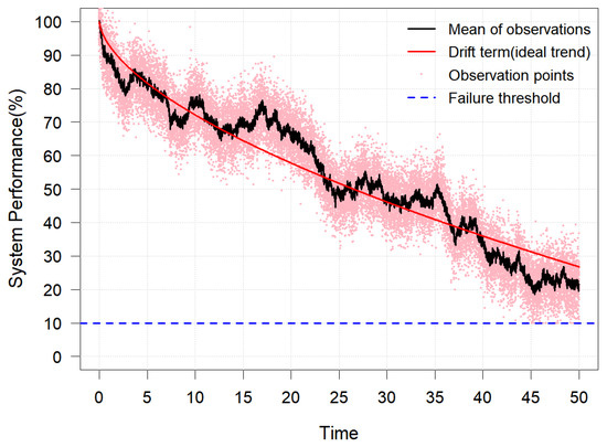
Figure 1.
Diagram of Wiener process with measurement error.
3.3. Reliability Assessment of Univariate Degradation Model
When the univariate degradation process is described by the Wiener process, the power-law time scale transformation function is used as an example for simplifying the presentation. Under the condition of Equation (1), the exact distribution of the first passage time is difficult to obtain analytically. Therefore, this paper employs an approximate probability density function (PDF) that has been validated in the literature [46], as follows:
where is derived under the assumption that, if the Wiener process hits the threshold exactly at time t, then the probability that it had crossed the threshold before t is negligible.
When considering the measurement error ,
By the law of total probability, based on Lemma 3 in the literature [47], the PDF of the lifetime when considering the measurement error is derived:
According to the relation to the reliability function,
Here, the reliability function for the PC is obtained. Similarly, repeat the above steps for PCs to obtain all the independent reliability functions.
4. Vine Copula Reliability Assessment Model Based on Chatterjee Correlation Coefficient
In this section, with the theory of the Chatterjee correlation coefficient and Vine copula, corresponding reliability assessments of the multiple indicators system are introduced.
4.1. The Theory of Chatterjee Correlation Coefficient
As simple as the classical coefficients, the correlation coefficient proposed by Chatterjee (referred to as the Chatterjee correlation coefficient in this paper) consistently estimates some measure of the dependence between variables. This dependence measure is 0 if and only if the variables are independent, and 1 if and only if one variable is a measurable function of the other. It is 0 if and only if the variables are independent and 1 if and only if one variable is a measurable function of the other. It is worth noting that the primary advantage of the Chatterjee coefficient lies in its asymmetric nature between and . That is to say, is a measure of whether is a function of , not just whether one of the variables is a function of the other. It does not rely on assumptions of linear or monotonic relationships between variables, and is able to measure the difference in dependency strength between “ is a function of ” and “ is a function of ”. This would be more consistent with scenarios in real physical systems where causal or driving relationships may exist between variables.
Let be a pair of random variables, where is not a constant. Let be a pair of i.i.d. variables, where . We assume that there is no equality among either ’s or ’s and rearrange the data as such that . Since there is no equality between ’s, this is the only permutation. Let be the rank of ; that is, the number of is such that . Then, the correlation coefficient is defined as follows:
If there are equalities among ’s, then break them uniformly and randomly by an increasing rearrangement as described above. is defined as before, and is also defined such that the number of makes . For this case, is defined as follows:
Similar to the classical correlation coefficients, Chatterjee correlation coefficient has a simple asymptotic theory under the independence assumption [43]: if is not a constant, then as , converges to a definite limit:
where is the law of . This limit belongs to the interval [0, 1]. The larger the value, the more likely it is that is a measurable function of .
Inspired by , the conditional Chatterjee correlation coefficient is an extension in the conditional dependence scenario. It is able to quantify the nonlinear, nonmonotonic conditional dependence between random variables and when given , which is difficult to do with the traditional correlation coefficient. In addition, this concept is able to capture localized patterns of dependence between variables by embedding nonparametric correlation measures in the framework of conditional distributions. Given , the conditional correlation coefficient of and is defined as follows [48]:
where is the amount of data. For each , represents the subscript of that is closest to . As with the rules for the definition of , if there are equalities, there are uniform breaks at random. represents the subscript of the closest to , and the distance is measured in terms of the normalized Euclidean distance. , defined as before, is the rank of ; i.e., the number of is such that . For the mathematical derivation and more details of Chatterjee correlation coefficient and conditional Chatterjee correlation coefficient, see references [43,48].
4.2. The Foundation of Vine Copula
The copula function is a link function that measures the correlation between two random variables. In Sklar theorem, with copula function, the marginal distributions of multiple variables can be linked into a multivariate joint distribution. It is defined as follows: let be an n-dimensional joint distribution function with marginal distribution functions , where and . Then, there exists a copula function satisfying the following equation:
In the high-dimensional case, the parameter estimation of copula function is more difficult. Thus, Vine copula was proposed to decompose the high-dimensional copula density function into the product of pair-copulas. The joint distribution function of any multivariate variable can be expressed by the following equation:
The structure of the n-dimensional copula density function is not unique. In fact, there are n!/2 pair-copula models that can be constructed. Therefore, in 2001, Bedford and Cooke proposed the concept of the R Vine copula, which is to use the structure of a tree to represent the linkage between variables. R Vine copula consists of trees, edges, and nodes between edges. Each edge is a pair-copula function, and different linking methods result in different structures. For example, in 2009, Aas et al. [49] constructed C Vine copula and D Vine copula, which are special cases of R Vine copula. C Vine copula has only one center node connected to other edges in each tree; that is, there is a unique root node. In contrast, D Vine copula is a parallel structure formed by connecting each variable two by two sequentially. Compared with the above two structures, R Vine copula is more universal because it does not restrict the method of connecting variables. Taking five variables as an example, the structure diagrams of the three concepts are shown in Figure 2, Figure 3 and Figure 4, respectively.
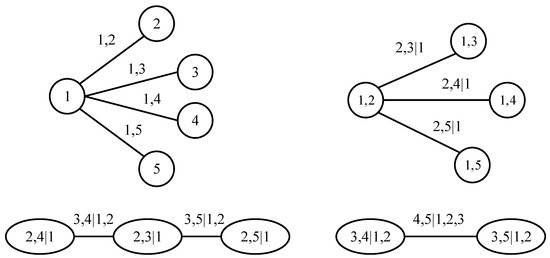
Figure 2.
Structure of C Vine copula.
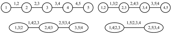
Figure 3.
Structure of D Vine copula.
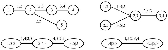
Figure 4.
Structure of R Vine copula.
4.3. Inference of Vine Copula Based on Chatterjee Correlation Coefficient
In view of the excellent performance of the Chatterjee correlation coefficient, it is introduced into Vine copula modeling. The modeling is mainly divided into two parts. The first part is to construct a reasonable tree structure for Vine copula, and the second part is to infer the joint distribution based on Vine copula. The flow chart is shown in Figure 5.
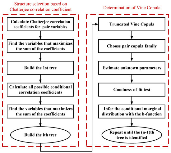
Figure 5.
Flowchart of the proposed Vine copula modeling process.
The three steps for the selection of tree structures are as follows:
Step 1 Calculate Chatterjee correlation coefficients for all possible pair variables according to Section 4.1.
Step 2 For each variable , find the Xi that maximizes , and all pair variables that make up the first tree are selected. Then, connect them to determine the structure of the first tree.
Step 3 Calculate the conditional Chatterjee correlation coefficients for all possible pair variables on the basis of the first tree construction (as shown in Section 4.1 for details) and select the pair variables that maximize the sum of the conditional Chatterjee correlation coefficient to construct the second tree. Similarly, repeat the inference and calculation until all tree structures are determined.
Vine copula represents the dependencies between multiple variables through a type of vine structure. In Tree 1, each node represents a variable; each edge represents a pairwise relationship between two variables. The appropriate pair-copulas need to be chosen to characterize the dependencies between these variables. The most popular ones are Gaussian copula, Student copula, Frank copula, and Gumbel copula. In this paper, based on the Akaike information criterion (AIC), the pair copula function that minimizes the AIC value is selected as the link function of two variables, as shown in Section 5.2. However, after Tree 2, the nodes no longer represent the original variables directly, but rather the edges; that is, the conditional variables are calculated by the h-function. These new edges instead represent conditional dependencies between two conditional variables given one or more other variables.
Given , if the random variable obeys the distribution , and the random variable obeys the distribution , then the corresponding conditional joint distribution is
The distribution function is obtained from the h-function,
Similarly, can be obtained. By analogy, all conditional distribution functions can be determined.
Thus, for a given condition set and edge set, the corresponding joint distribution function is allowed to be decomposed as follows:
where is the number of variables. The tree is represented by , and is the set of all edges. For , and are the two variables connected to the edges, and is the set of all conditional variables. The corresponding copula distribution function is denoted as , and is the variable indexed by the set .
4.4. Reliability Assessment of Multivariate Degradation System
For the degradation process , , and the lifetime is defined as the moment when the amount of degradation reaches the threshold for the first time, characterized as follows:
Obviously, the reliability at moment is defined as the probability that the failure threshold is not reached at present,
Therefore, the reliability of a binary degradation system can be derived as follows:
The reliability of the ternary degradation system is
By analogy, for the n-dimensional system, the reliability is given below:
where denotes all possible combinations of variables selected from . In particular, when the degradation processes are independent of each other, the reliability of the n-dimensional system is the product of the marginal reliability functions,
5. Parameter Estimation and Statistical Inference
In this section, maximum likelihood estimation (MLE) is employed to estimate unknown parameters from the previous two chapters. Due to the difficulty and complexity of estimating all the parameters holistically by performing MLE, a popular two-stage inference method, inference function for margins (IFM), is available to reduce the computational burden. It is divided into the following two subsections:
5.1. Parameter Estimation of Univariate Degradation Model
For simplicity of presentation, the subscript representing the PC is ignored. The unknown parameter is solved by performing the maximum likelihood estimation based on the state space model developed in Section 3.2. According to the assumption of independence between samples, the likelihood function of the parameter can be expressed as follows:
Based on the properties of the Wiener process, it can be seen that obeys a multivariate normal distribution with mean matrix and covariance matrix , where is an identity matrix,
For ease of computation, the likelihood function is taken to be logarithmic, yielding
Taking the first-order partial derivatives of to 0 yields the equation:
Substituting Equation (13) into Equation (12) yields the cross-sectional likelihood function. The parameter that maximizes the cross-section likelihood function is found by the three-dimensional search algorithm, and then by substituting them into Equation (13), is obtained.
5.2. Statistical Inference of Vine Copula
The purpose of this subsection is to further obtain the Vine copula function parameters based on the marginal distribution parameters obtained in the previous section. According to the graphical representation of R Vine copula in Figure 4, the n-dimensional multivariate structure can be described as n-1 trees, where each tree can be described as a product of various pair-copula. The calculation of the joint distribution function of the proposed model can be divided into five steps.
Step 1: Select the candidate copula function family for Tree 1.
Based on the obtained marginal distribution functions, select a set of the candidate copula function family for the pair variables in Tree 1. The set is required to cover the types of symmetric dependence (e.g., Gaussian copula) and asymmetric dependence (e.g., Clayton copula, Gumbel copula) in order to fully capture the potential dependence patterns of the variable pairs.
Step 2: Construct the likelihood function for Tree 1 and estimate the parameters.
The parameters of the pair-copulas in Tree 1 are estimated using the maximum likelihood estimation (MLE) method. In details, for each pair of variables in Tree 1 and the corresponding candidate copula family, construct the log-likelihood function with respect to the unknown parameters . Given covariate , assuming that the conditional dependence of the pair variable is modeled by the copula density , then the log-likelihood function is defined as:
where denotes, for the sample of the variable , the value of the conditional distribution function with the covariate is . The maximum likelihood estimation is obtained by solving through numerical optimization algorithms.
Step 3: Select the optimal model for Tree 1 based on the AIC.
The Akaike information criterion (AIC) is computed for each candidate copula of all pair variables, defined as:
where is the number of model parameters and log-LF is the maximum log-likelihood function value. The copula function with the smallest AIC value is selected as the optimal model for each pair variable to balance the model fit goodness-of-fit and complexity. Combining them results in the optimal model for Tree 1.
AIC is a measure of the relative quality of statistical models, based on information theory. The goodness-of-fit (log-LF value) and the complexity of the model (number of parameters) are combined to avoid overfitting. Specifically, the first term 2(log-LF) indicates the goodness-of-fit of candidate model: the larger the log-likelihood value (better fit), the smaller the value of this term. The second term is the penalty for model complexity: the more parameters, the greater the penalty. Therefore, a relative comparison is made among several candidate models and the model with the smallest AIC value is selected. It should be noted that the size of the AIC value has no absolute significance, while it serves solely as a basis for comparing the relative merits of different models.
Step 4: Calculate the conditional distribution function and build Tree 2 nodes.
Based on the optimal copula model of Tree 1, calculate the conditional distribution function using Equation (9):
This conditional distribution function will be used as a node variable in Tree 2 for modeling higher-order conditional dependency structures. For example, the conditional distributions of variable pair and , and , may form a new pair variable in Tree 2.
Step 5: Estimate parameters and select models for Subsequent Trees recursively.
From Tree 2 to Tree n-1, recursively perform the following procedures:
- For pair variables in the current tree, select candidate copula families and estimate their parameters;
- Choose the optimal copula based on AIC;
- Compute higher-order conditional distribution functions and transfer them to the next tree.
Ultimately, copula functions of all trees collectively form an integrated decomposition structure of Vine copula joint distribution. The joint density can be expressed as the product of all pair-copula density functions.
6. Numerical Example
This section presents a numerical example to validate the proposed methodology, utilizing the C-MAPSS dataset published by NASA [50]. This dataset records aero-engine operational data and is extensively used in studies of aero-engine degradation mechanisms. Each set consists of three subsets: the training set, the test set, and the RUL set. Initial engine operation is characterized by varying levels of initial losses and manufacturing variability while being considered to be in a normal state. Eventually, the system deteriorates until an operational failure occurs. The C-MAPSS dataset is a multivariate time series containing data collected from 21 sensors, only some of which exhibit strong monotonicity, making it suitable for this study and highlighting its practical relevance. In addition, a subset of sensor data is selected for multivariate analysis in this section, which is also in line with the actual situation. Taking Sensor 7 (P30, total pressure at the outlet of the high-pressure pressurizer), Sensor 9 (NC, core machine speed) and Sensor 12 (PHI, the ratio of the fuel flow rate to P30) as PC1, PC2, and PC3, respectively. Individuals 1, 15, and 33 in the FD001 dataset are selected for the reliability assessment, denoted as Individuals 1, 2, and 3, respectively. Their degradation trajectories are shown in Figure 6.
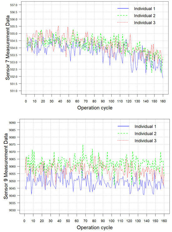
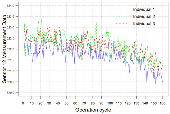
Figure 6.
Sensor degradation trajectory of FD001.
Figure 6 reveals that the selected sensor trajectories exhibit strong nonlinear characteristics. Therefore, based on Wiener process, a power-law function is used as the time scale transformation function to describe its degradation trend. Without loss of generality, errors occur in the measurement process due to the influence of materials, environment and other factors. Therefore, it is appropriate to use a state space model that takes into account the measurement error for the fitting of the marginal degradation model. To justify the model’s statistical assumptions, we first verify the normality of the degradation data. The Shapiro–Wilk hypothesis test (SW test, significance level α = 0.05) is used for quantitative validation, supplemented by graphical diagnostic methods (quantile-quantile (QQ) plots and frequency histograms) to visually assess distribution patterns. Table 1 shows that the p-values of the SW test for three PCs are beyond the significance level. Meanwhile, from Figure 7, there is no aggregation bias in the residuals of QQ plots, and the symmetry of histogram distribution is significant. Therefore, statistical characteristics of the degradation data for each PC have no significant deviation from normal distribution.

Table 1.
Results of the Shapiro-Wilk test.
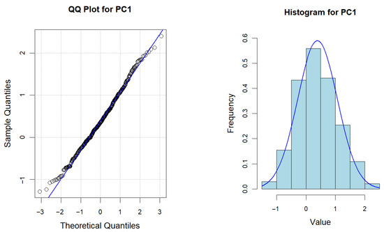
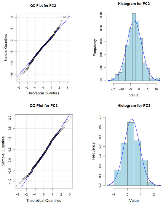
Figure 7.
QQ plots and frequency histograms for each PC. (The blue line indicates the fit to the data).
According to the steps in Section 5.1, parameters are estimated by MLE, with results summarized in Table 2. In order to compare the applicability of model M0 (considering measurement error) with model M1 (not considering measurement error), two quantitative indicators, log-LF value, and AIC are given.
Table 2.
Comparative results of parameter estimation.
As evident from Table 2, both evaluation criteria favor model M0 over M1. This indicates that M0 provides a superior fit for describing the sample degradation processes and yields a more accurate product reliability analysis.
Based on the obtained marginal degradation distribution, the Vine copula proposed in Section 4 is established and the Chatterjee correlation coefficients between pair variables are calculated in Table 3. It can be seen that the dependence between PC1 and PC3 (0.355) is the strongest. The correlation coefficient between PC2 and PC1 (0.109) is greater than the correlation coefficient between PC2 and PC3 (0.060), indicating that PC2 is relatively dependent on PC1. In accordance with the principle of the maximum spanning tree, the Vine copula structure is determined as Vine1 (). Similarly, Kendall correlation coefficients between pair variables can be obtained in Table 4. The Kendall correlation coefficient between PC1 and PC3 (0.489) is also the strongest. The Vine copula structure determined by the Kendall correlation coefficient is thus obtained as Vine2 ().
Table 3.
Chatterjee correlation coefficients for pair variables.
Table 4.
Kendall correlation coefficients for pair variables.
A comparison of Table 3 and Table 4 shows that the strongest dependence is consistently identified between PC1 and PC3, confirming the robustness of this relationship across different correlation measures. However, the difference lies in the relative dependence of PC2. The Chatterjee correlation coefficient points to a relative dependence of PC2 on PC1, while the Kendall correlation coefficient shows a relative dependence on PC3. This disagreement may stem from the fact that the two correlation coefficients capture the dependence in different ways.
The Chatterjee correlation coefficient offers distinct advantages in capturing nonlinear and asymmetric dependence structures between variables. According to the definition in Section 4.1, it distinguishes between “explanatory variables” and “dependent variables”. calculates the fluctuation range of the rank of dependent variable , as it changes sequentially with explanatory variable , focusing solely on “the effect of ’s sequence on ’s rank.” Swapping and may yield different fluctuations in rank, leading to the difference between and . In contrast, Kendall coefficient measures symmetric, non-directional rank concordance. It assesses the general monotonic synergy between variables, and its value is invariant to swapping and .
As illustrated in Table 3, the dependence of PC2 on PC1 (0.109) differs from that of PC1 on PC2 (0.103), revealing inherent asymmetry in their relationship. The asymmetry stems from the system’s physical mechanisms. For example, changes in PC2 (core machine speed) may tend to “drive” changes in PC1 (P30 pressure) rather than strict bidirectional synchronization. Table 4 exemplifies the limitation of the Kendall coefficient: the degree to which PC2 depends on PC1 (0.234) is the same as the degree to which PC1 depends on PC2 (0.234). Such symmetrical constraints may lead to oversimplified or inaccurate representations of complex variable interactions. The capacity to discern directional disparities makes the Chatterjee coefficient both flexible and precise for dependency analysis. This facilitates more accurate depictions of causal or driving relationships for modern analytical applications. For instance, the core machine speed may control exhaust temperature systemically, but the reverse is not true. Accurate quantification of such asymmetric dependency is critical in system health management. For instance, knowing that PC2 exerts stronger driving influence over PC1 allows monitoring exceptions in PC2 to provide earlier warnings of potential PC1 faults. This enables maintenance planning to prioritize resource allocation toward components more critical to system reliability, thereby achieving more responsive and cost-effective predictive maintenance.
Maximum likelihood estimation is applied to pair-copula for model selection and parameter estimation. The model with the smallest AIC is selected as the optimal model. Thus, for Vine1, the types of copula functions connecting PC1 with PC2 and PC1 with PC3 in Tree 1 are selected as Gaussian and Joe, respectively. The copula in Tree 2 is selected as Rotated Clayton (90 degree), and the estimated parameters are shown in Table 5. The log-likelihood function value (shortened to log-LF in the Table 5), AIC, and the Vuong test statistic V are used as model comparison indicators.
Table 5.
Parameter estimation of various copula. (The blue element represents the central variable).
To evaluate Vine copula proposed in this paper (denoted as Vine1), a multidimensional comparison experiment is designed. The experimental object contains five types of models: (1) Vine1 determined by Chatterjee coefficients; (2) the comparison model Vine2 determined by Kendall correlation coefficients (literature [42]); and (3) three multivariate Copula models (Gaussian Copula, t-Copula, and Joe Copula) that have the same variable structure as Vine1. Vine1 (with mixed copula) is compared with all other models. Table 5 shows numbers of parameters, log-likelihood values, AIC, and results of the Vuong tests (test statistics and p-values in parentheses) for all models. The Vuong test is a log-likelihood ratio-based statistic used to compare the goodness-of-fit of two competing models. The positive values of Vuong test statistics indicate that the test favors the proposed model over the respective alternative model (inconclusive region at the 5%-level: [−1.96, 1.96]). The gray dashed line in Figure 8 corresponds to level 1.96.
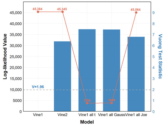
Figure 8.
Comparison of goodness-of-fit for different Vine copulas.
As seen in Table 5 and Figure 8, despite the small difference in log-likelihood values between Vine1 and Vine2, the Vuong test statistic (6.37) is significantly greater than 1.96. Thereby, there is a systematic difference in fit between the two models at the significance level α = 0.05. It can be concluded that Vine1 fits the data better and performs better than Vine2. On the other hand, Vine1 with mixed copula is preferred to multivariate copulas having the same structure as Vine1. In other words, Vine1 can better describe the dependencies between multiple failure processes. Based on the constructed optimal model and parameters, the reliability assessment of the system is carried out, and the reliability curve of the system is obtained as shown in Figure 9.
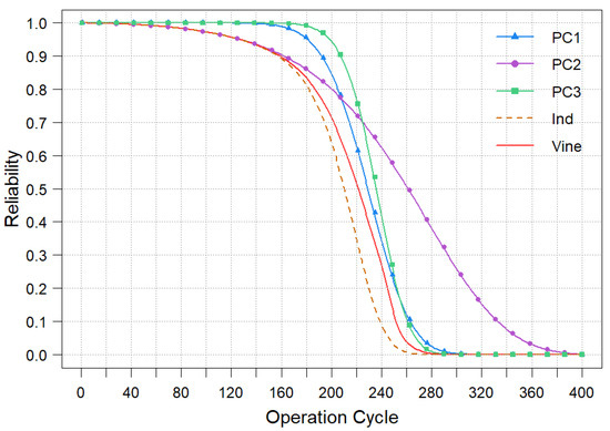
Figure 9.
System reliability curve with three variables.
Finally, the reliability of the aero-engine multivariate system considering dependence is compared with the reliability under the independence assumption. From Figure 9, the reliability curve considering dependence is smaller than the minimum value of individual PCs and larger than the case of mutual independence. That is, the independence assumption may underestimate the system’s reliability. This situation is not uncommon in many engineering applications. Therefore, it is more reasonable to apply the proposed method for evaluating product reliability when there are multiple dependent PCs.
Figure 9 illustrates the reliability curves of different models. PC1, PC2 and PC3 represent the reliability curves of different failure processes, while Ind and Vine represent the reliability curves of the independent model and the Vine1-based model, respectively. As expected, all models show near-perfect reliability at the start of the operational cycle. As the operating cycle increases, the reliability of PC1 and PC2 decreases rapidly, while PC3 decreases relatively slowly. This indicates that the failure process represented by PC1 and PC2 has a more significant effect on the system reliability. The independent model (Ind), which is a simple product of the marginal reliability, produces a curve that decreases at an intermediate rate. However, by failing to account for the dependencies, it systematically underestimates the system’s reliability compared to the proposed Vine1, particularly during the mid-to-late stages of the life cycle. The superior performance of the Vine1 model (red curve) stems from its ability to accurately characterize the complex dependencies among the failure processes, leading to a more realistic and trustworthy system-level reliability assessment.
The performance difference fundamentally arises from the flexible and accurate dependency modeling enabled by Vine1. By selectively employing Gaussian, Joe, and Rotated Clayton copulas across its structure, Vine1 can tailor the dependence capture to each variable pair, a flexibility that the rigid independence assumption completely lacks.
It is worth discussing that the computational burden increases with the number of PCs, primarily from two stages: Vine copula structure selection and pair copula parameter estimation. Vine copula structure selection requires computing the Chatterjee coefficients and conditional Chatterjee coefficients, with a complexity of O(n2). Additionally, parameter estimation for O(n2) pair copula functions, coupled with model selection by AIC, further increases the overall computational cost. To mitigate this issue and enhance the method’s practicality in high-dimensional data, several strategies can be employed. At the algorithmic level, high-dimensional variables can be divided into low-dimensional subgroups by hierarchical aggregation methods. Sub-Vine copulas are constructed for each subgroup, and the submodules are integrated as marginal distributions into higher-level copulas. This effectively treats an unwieldy high-dimensional problem as a series of manageable low-dimensional problems. Dimensionality reduction techniques, like principal component analysis, can also be applied during preprocessing to identify a critical subset of PCs. Regarding computational resources, the inherent parallelism in Vine copulas, where pair copulas at the same tree level can be estimated independently, makes it highly suitable for parallel computing frameworks (e.g., GPU acceleration), significantly reducing processing time. Despite the complexity, such strategies render the method feasible for medium-dimensional systems in typical engineering applications. Future work will focus on developing more efficient and scalable inference algorithms.
7. Conclusions
This paper improved the reliability modeling of multivariate degradation systems based on Vine copula and the Chatterjee correlation coefficient while considering multiple sources of uncertainty. It provided a useful tool for reliability assessment and maintenance strategy development for products with multiple performance characteristics. Through systematic research and analysis, the main results are as follows:
- (1)
- The marginal degradation model was described by a general Wiener process containing two sources of uncertainty, and the corresponding parameter estimation method was provided. The nonparametric coefficient, the Chatterjee correlation coefficient, was also introduced to capture the nonlinear and asymmetric dependence among multivariate variables. A unified framework for uncertainty analysis of degradation mechanisms and decoupling of variable coupling effects was constructed. This method broke through the limitation of the traditional correlation coefficient (Kendall coefficient) on monotonic symmetric relationships.
- (2)
- The multivariate joint degradation model was constructed by the Vine copula technique, and the structure selection was optimized by the goodness-of-fit criterion. The numerical example showed that the reliability curve lies between two extreme assumptions of complete independence and complete dependence of variables, which is consistent with the physical properties of partial correlations in engineering practice.
- (3)
- The interpretability of reliability assessment model was enhanced by constructing a degradation dependence network using statistical models, such as Vine copula.
The research results provided an improved paradigm for the reliability assessment of complex systems. Nonetheless, the proposed approach has limitations that present pathways for future work. Its performance is contingent on substantial, high-quality data for robust parameter estimation, and it assumes static dependencies, which may not capture dynamic interactions under time-varying operational profiles. Future research will thus focus on (1) enhancing computational scalability and efficiency for high-dimensional data; (2) extending the framework to model dynamic dependencies and incorporate additional uncertainties like random shocks; and (3) developing data-efficient estimation techniques to improve applicability in small sample scenarios.
Author Contributions
Conceptualization, J.T. and M.J.; methodology, M.J. and J.T.; software, M.J.; validation, M.J. and Y.M.; formal analysis, J.T. and M.J.; investigation, M.J.; resources, J.T.; data curation, M.J.; writing—original draft preparation, M.J.; writing—review and editing, J.T., M.J. and Y.M.; visualization, M.J. and Y.M.; supervision, J.T.; project administration, J.T.; funding acquisition, J.T. All authors have read and agreed to the published version of the manuscript.
Funding
This research was funded by Humanistic Social Research Planning Fund of the Education Ministry of China, grant No.20XJAZH009, and National Social Science Fund of China, grant No.23BTJ010.
Data Availability Statement
The dataset used in this paper is available from the NASA website.
Acknowledgments
The authors express their sincere thanks to the anonymous referees for their insightful comments and constructive suggestions, which have led to a substantial improvement for this paper. We would also like to thank the Editor in Chief for all his efforts handling the paper.
Conflicts of Interest
Author Mr. Yamin Mao was employed by CETC Rong Wei Electronic Technology Co., Ltd. The remaining authors declare that the research was conducted in the absence of any commercial or financial relationships that could be construed as a potential conflict of interest.
Nomenclature
| Number of degradation performance characteristics (PCs) | |
| Number of discrete measurement time points | |
| Number of samples | |
| discrete measurement time for PC of sample | |
| Measurement data at time | |
| Column vector composed of | |
| Column vector composed of | |
| / | The true degradation of PC for sample at discrete measurement time point |
| The observation of PC for sample at discrete measurement time point | |
| Normal distribution with mean and variance | |
| Initial degradation value of the population for PC | |
| Time scale function of degradation process | |
| Standard Brownian motion | |
| Drift coefficient of degradation process | |
| Diffusion coefficient of degradation process | |
| Measurement error of degradation process | |
| Standard deviation of measurement error | |
| Parameter vector in state space model | |
| Difference between and | |
| Difference between and | |
| Mean of random variable in parentheses | |
| Approximate lifetime PDF corresponding to PC (not considering ) | |
| Failure threshold of PC | |
| Approximate conditional lifetime PDF given the measurement error | |
| Approximate lifetime PDF corresponding to PC (considering ) | |
| Probability density function (PDF) of random variable in parentheses | |
| Lifetime PDF corresponding to PC (considering ) | |
| Reliability function corresponding to PC | |
| Chatterjee correlation coefficient to measure the degree of dependence of random variable on | |
| Rank of , number of such that | |
| Number of such that | |
| Limit of | |
| Given , conditional Chatterjee correlation coefficient between and | |
| Index of closest to | |
| Index of closest to | |
| Probability of event in parentheses | |
| Distribution function of the variable in parentheses | |
| Copula function connecting random variables in parentheses | |
| Set of all trees | |
| Edge of tree | |
| Set of all edges | |
| Two variables connected by edge | |
| Set of all conditional variables | |
| Lifetime corresponding to PC, time when the degradation value first reaches the threshold | |
| Mean matrix of sample | |
| Covariance matrix of sample | |
| Custom symmetric matrix for calculating | |
| / | Likelihood /log-likelihood function with parameter in parentheses |
| Number of unknown model parameters |
References
- Liu, Q.; Zhuo, J.; Lang, Z.; Qin, S. Perspectives on data-driven operation monitoring and self-optimization of industrial processes. Acta Autom. Sin. 2018, 44, 1944–1956. [Google Scholar]
- Li, X.; Duan, F.; Mba, D.; Bennett, I. Multidimensional prognostics for rotating machinery: A review. Adv. Mech. Eng. 2017, 9, 1–20. [Google Scholar] [CrossRef]
- Sun, F.; Fu, F.; Liao, H.; Xu, D. Analysis of multivariate dependent accelerated degradation data using a random-effect general Wiener process and D-vine Copula. Reliab. Eng. Syst. Saf. 2020, 204, 107168. [Google Scholar] [CrossRef]
- Zhang, H.; Zhou, D.; Chen, M.; Shang, J. FBM-Based Remaining Useful Life Prediction for Degradation Processes with Long-Range Dependence and Multiple Modes. IEEE Trans. Reliab. 2019, 68, 1021–1033. [Google Scholar] [CrossRef]
- Liang, X.; Liu, Y.; Chen, S.; Li, X.; Jin, X.; Du, Z. Physics-informed neural network for chiller plant optimal control with structure-type and trend-type prior knowledge. Appl. Energy 2025, 390, 125857. [Google Scholar] [CrossRef]
- Wang, Y.; Kang, R.; Chen, Y. Belief reliability modeling for the two-phase degradation system with a change point under small sample conditions. Comput. Ind. Eng. 2022, 173, 108697. [Google Scholar] [CrossRef]
- Yao, Y.; Han, T.; Yu, J.; Xie, M. Uncertainty-aware deep learning for reliable health monitoring in safety-critical energy systems. Energy 2024, 291, 130419. [Google Scholar] [CrossRef]
- Cheng, Y.; Qv, J.; Feng, K.; Han, T. A Bayesian adversarial probsparse Transformer model for long-term remaining useful life prediction. Reliab. Eng. Syst. Saf. 2024, 248, 110188. [Google Scholar] [CrossRef]
- Ghorbani, S.; Salahshoor, K. Estimating remaining useful life of turbofan engine using data-level fusion and feature-level fusion. J. Fail. Anal. Prev. 2020, 20, 323–332. [Google Scholar] [CrossRef]
- Lei, Y.; Li, N.; Guo, L.; Li, N.; Yan, T.; Lin, J. Machinery health prognostics: A systematic review from data acquisition to RUL prediction. Mech. Syst. Signal Process. 2018, 104, 799–834. [Google Scholar] [CrossRef]
- Ounoughi, C.; Yahia, S.B. Data fusion for ITS: A systematic literature review. Inf. Fusion 2023, 89, 267–291. [Google Scholar] [CrossRef]
- Liang, Q.; Yang, C.; Lin, S.; Hao, X. Multi-source information grey fusion method of torpedo loading reliability. Ocean Eng. 2021, 234, 109303. [Google Scholar] [CrossRef]
- Han, D.; Tian, J.; Xue, P.; Shi, P. A novel intelligent fault diagnosis method based on dual convolutional neural network with multi-level information fusion. J. Mech. Sci. Technol. 2021, 35, 3331–3345. [Google Scholar] [CrossRef]
- Duan, L.; Zhao, F.; Wang, J.; Wang, N.; Zhang, J. An integrated cumulative transformation and feature fusion approach for bearing degradation prognostics. Shock Vib. 2018, 2018, 9067184. [Google Scholar] [CrossRef]
- Ardeshiri, R.R.; Liu, M.; Ma, C. Multivariate stacked bidirectional long short term memory for lithium-ion battery health management. Reliab. Eng. Syst. Saf. 2022, 224, 108481. [Google Scholar] [CrossRef]
- Wang, D.; Liu, K. An integrated deep learning-based data fusion and degradation modeling method for improving prognostics. IEEE Trans. Autom. Sci. Eng. 2023, 21, 1713–1726. [Google Scholar] [CrossRef]
- Li, Q.; Ma, Z.; Li, H.; Liu, X.; Guan, X.; Tian, P. Remaining useful life prediction of mechanical system based on performance evaluation and geometric fractional Lévy stable motion with adaptive nonlinear drift. Mech. Syst. Signal Process. 2023, 184, 109679. [Google Scholar] [CrossRef]
- Gaw, N.; Yousefi, S.; Gahrooei, M.R. Multimodal data fusion for systems improvement: A review. IISE Trans. 2022, 54, 1098–1116. [Google Scholar] [CrossRef]
- Wen, P.; Li, Y.; Chen, S.; Zhao, S. Remaining useful life prediction of IIoT-enabled complex industrial systems with hybrid fusion of multiple information sources. IEEE Internet Things J. 2021, 8, 9045–9058. [Google Scholar] [CrossRef]
- Nelsen, R.B. An Introduction to Copulas; Springer: Berlin/Heidelberg, Germany, 2006. [Google Scholar]
- Yang, C.; Gu, X.; Zhao, F. Reliability analysis of degrading systems based on time-varying copula. Microelectron. Reliab. 2022, 136, 114628. [Google Scholar] [CrossRef]
- Zhang, Z.; Si, X.; Hu, C.; Lei, Y. Degradation data analysis and remaining useful life estimation: A review on Wiener-process-based methods. Eur. J. Oper. Res. 2018, 271, 775–796. [Google Scholar] [CrossRef]
- Shen, Y.; Shen, L.; Xu, W. A Wiener-based degradation model with logistic distributed measurement errors and remaining useful life estimation. Qual. Reliab. Eng. Int. 2018, 34, 1289–1303. [Google Scholar] [CrossRef]
- Dai, X.; Qu, S.; Sui, H.; Wu, P. Reliability modelling of wheel wear deterioration using conditional bivariate gamma processes and Bayesian hierarchical models. Reliab. Eng. Syst. Saf. 2022, 226, 108710. [Google Scholar] [CrossRef]
- Song, K. Multivariate degradation modeling and reliability evaluation using gamma processes with hierarchical random effects. J. Comput. Appl. Math. 2025, 465, 116591. [Google Scholar] [CrossRef]
- Fang, G.; Pan, R.; Wang, Y. Inverse Gaussian processes with correlated random effects for multivariate degradation modeling. Eur. J. Oper. Res. 2022, 300, 1177–1193. [Google Scholar] [CrossRef]
- Ye, Z.S.; Chen, N. The inverse Gaussian process as a degradation model. Technometrics 2014, 56, 302–311. [Google Scholar] [CrossRef]
- Zhuang, L.; Xu, A.; Wang, Y.; Tang, Y. Remaining useful life prediction for two-phase degradation model based on reparameterized inverse Gaussian process. Eur. J. Oper. Res. 2024, 319, 877–890. [Google Scholar] [CrossRef]
- Rodriguez-Picon, L.A. Reliability assessment for systems with two performance characteristics based on gamma processes with marginal heterogeneous random effects. Eksploat. I Niezawodn. 2017, 19, 8–18. [Google Scholar] [CrossRef]
- Pang, T.; Yu, T.; Song, B. RUL prediction for bivariate degradation process considering individual differences. Measurement 2023, 218, 113156. [Google Scholar] [CrossRef]
- Si, X.S.; Wang, W.; Hu, C.H.; Zhou, D.H. Estimating remaining useful life with three-source variability in degradation modeling. IEEE Trans. Reliab. 2014, 63, 167–190. [Google Scholar] [CrossRef]
- Si, X.S. An adaptive prognostic approach via nonlinear degradation modeling: Application to battery data. IEEE Trans. Ind. Electron. 2015, 62, 5082–5096. [Google Scholar] [CrossRef]
- Hao, S.; Yang, J.; Berenguer, C. Degradation analysis based on an extended inverse Gaussian process model with skew-normal random effects and measurement errors. Reliab. Eng. Syst. Saf. 2019, 189, 261–270. [Google Scholar] [CrossRef]
- Joe, H. Multivariate models and multivariate dependence concepts. CRC Press: Boca Raton, FL, USA, 1997.
- Bedford, T.; Cooke, R.M. Vines--a new graphical model for dependent random variables. Ann. Stat. 2002, 30, 1031–1068. [Google Scholar] [CrossRef]
- Fang, G.; Pan, R. On multivariate copula modeling of dependent degradation processes. Comput. Ind. Eng. 2021, 159, 107450. [Google Scholar] [CrossRef]
- Wen, B.; Xiao, M.; Zhao, X.; Ge, Y.; Li, J.; Zhu, H. Multivariate degradation system reliability analysis with multiple sources of uncertainty. Comput. Ind. Eng. 2023, 185, 109666. [Google Scholar] [CrossRef]
- Xu, D.; Xing, M.; Wei, Q.; Qin, Y.; Xu, J.; Chen, Y.; Kang, R. Failure behavior modeling and reliability estimation of product based on vine-copula and accelerated degradation data. Mech. Syst. Signal Process. 2018, 113, 50–64. [Google Scholar] [CrossRef]
- Ismail, M.S.; Masseran, N. Risk assessment for extreme air pollution events using vine copula. Stoch. Environ. Res. Risk Assess. 2024, 38, 2331–2358. [Google Scholar] [CrossRef]
- Bao, X.; Li, J.; Shen, J.; Chen, X.; Zhang, C.; Cui, H. Comprehensive multivariate joint distribution model for marine soft soil based on the vine copula. Comput. Geotech. 2025, 177, 106814. [Google Scholar] [CrossRef]
- Czado, C. Vine copula based structural equation models. Comput. Stat. Data Anal. 2025, 203, 108076. [Google Scholar] [CrossRef]
- Dissmann, J.; Brechmann, E.C.; Czado, C.; Kurowicka, D. Selecting and estimating regular vine copulae and application to financial returns. Comput. Stat. Data Anal. 2013, 59, 52–69. [Google Scholar] [CrossRef]
- Chatterjee, S. A new coefficient of correlation. J. Nonparametr. Stat. 2020, 32, 725–738. [Google Scholar] [CrossRef]
- Wu, B.; Zeng, J.; Shi, H.; Zhang, X.; Qin, Y. Remaining useful life prediction for multiple degradation indicators systems considering random correlation. Comput. Ind. Eng. 2023, 186, 109736. [Google Scholar] [CrossRef]
- Liu, S.; Jiang, H. Engine remaining useful life prediction model based on R-Vine copula with multi-sensor data. Heliyon 2023, 9, e17118. [Google Scholar] [CrossRef] [PubMed]
- Sun, F.; Liu, L.; Li, X.; Liao, H. Stochastic modeling and analysis of multiple nonlinear accelerated degradation processes through information fusion. Sensors 2016, 16, 1242. [Google Scholar] [CrossRef]
- Si, X.S.; Wang, W.; Hu, C.H.; Zhou, D.H.; Pecht, M.G. Remaining useful life estimation based on a nonlinear diffusion degradation process. IEEE Trans. Reliab. 2012, 61, 50–67. [Google Scholar] [CrossRef]
- Azadkia, M.; Chatterjee, S. A simple measure of conditional dependence. Ann. Stat. 2021, 49, 3070–3102. [Google Scholar] [CrossRef]
- Aas, K.; Czado, C.; Frigessi, A.; Bakken, H. Pair-copula constructions of multiple dependence. Insur. Math. Econ. 2009, 44, 182–198. [Google Scholar] [CrossRef]
- Saxena, A.; Goebel, K.; Simon, D.; Eklund, N. Damage propagation modeling for aircraft engine run-to-failure simulation. In Proceedings of the 2008 International Conference on Prognostics and Health Management, Denver, CO, USA, 6–9 October 2008; pp. 1–9. [Google Scholar]


Disclaimer/Publisher’s Note: The statements, opinions and data contained in all publications are solely those of the individual author(s) and contributor(s) and not of MDPI and/or the editor(s). MDPI and/or the editor(s) disclaim responsibility for any injury to people or property resulting from any ideas, methods, instructions or products referred to in the content. |
© 2025 by the authors. Licensee MDPI, Basel, Switzerland. This article is an open access article distributed under the terms and conditions of the Creative Commons Attribution (CC BY) license (https://creativecommons.org/licenses/by/4.0/).