Analyzing Rear-End Crash Counts on Ohio Interstate Freeways Using Advanced Multilevel Modeling

Abstract

This study presents a new modeling approach for rear-end crash counts on Ohio’s interstate freeways based on a dataset for 2021 that contains 2745 rear-end crashes. The analysis encompasses 20 interstate freeways, comprising 1833 homogeneous segments and extending over approximately 1313 miles. These interstate freeways exhibit varying safety performances, indicating a significant degree of heterogeneity. A unique rear-end crash risk rate was devised for each interstate, capturing diverse risk profiles. Three distinct models were developed: a standard negative binomial model, an uncorrelated two-level negative binomial model, and a correlated two-level negative binomial model. The correlated two-level negative binomial model demonstrated superior fit, as evidenced by the likelihood ratio test, Akaike information criterion, and Bayesian information criterion. The correlated two-level negative binomial model exhibited enhanced forecasting precision, as measured by the Root Mean Square Error. A significant finding is that the rear-end crash risk rate significantly improves the fit of the models. The study also reveals that rear-end crashes are expected to occur more frequently in urban segments of interstate freeways with high rear-end risk rates. However, rural segments experience no such significant variations in the rear-end crash risk rate. However, an increase in the inner shoulder width is associated with a decrease in expected rear-end crashes. This research offers a valuable methodology for modeling rear-end crashes on interstate freeways, providing insights into the contributing variables that could inform targeted safety improvements.

1. Introduction

Rear-end crashes are a common type of collision. Numerous studies have been conducted to understand and draw meaningful conclusions about these incidents. Typically, researchers focus on two primary goals: investigating contributing factors related to crash severity and modeling the frequency of crash occurrence. One study explored injury severity differences between front-vehicle occupants and rear-vehicle occupants involved in two-vehicle fatal rear-end crashes [1]. Using data from the Fatality Analysis Reporting System (FARS) for 2017 to 2019, the dataset was divided into two parts: one for front-vehicle occupants and another for rear-vehicle occupants. Three variants of multinomial logit models were applied separately to each dataset: a random parameter model, a random parameter model with heterogeneity in means, and a correlated parameter model with heterogeneity in means. The study found that the correlation between random parameters and heterogeneity in means significantly improved model fit, albeit by a small margin. The insights gained from this research are particularly relevant to understanding the differences in injury severity between occupants in front-vehicle and rear-vehicle collisions. Another study examined various factors contributing to rear-end collisions in urban environments. The findings indicate that elevated traffic flow and significant speed variance are strongly correlated with an increased potential for rear-end crashes [2]. A study conducted in Serbia revealed significant differences in youth perceptions and attitudes towards road safety between urban and rural areas [3]. A recent study analyzed 367,230 crashes using classification tree models [4]. The study found that rear-end crashes are more frequent in urban areas and major cities. However, while machine learning methods excel at classification and predictions, they are less effective in understanding the associations between predictors and the response variable.

Table 1. Examples of recent studies on injury severity in rear-end crashes.

Model Type	Focus	Year Article
Random parameters bivariate ordered probit model	Investigated the factors contributing to driver injury severity in rear-end crashes. Modeled the drivers’ severity in the same crash together by allowing for the correlation between the drivers involved. Allowed the parameters to vary across observations. Highlighted the importance of considering both within-crash correlation and unobserved heterogeneity in injury severity analysis.	2019 [5]
Random parameters ordered probit model	Studied the injury severity differences between car-strike-truck and truck-strike-car collisions. Found significant differences in contributing factors. Allowed parameters to vary across observations to account for unobserved heterogeneity.	2020 [6]
Random parameters ordinal probit model	Investigated factors contributing to injury severity in rear-end crashes at signalized intersections. Allowed parameters to vary across observations to account for unobserved heterogeneity.	2022 [7]
Random parameters logit model	Investigated factors contributing to injury severity in rear-end crashes on two freeways. Examined transferability and heterogeneity between two-vehicle and multi-vehicle crashes. Allowed parameters to vary across observations and accounted for heterogeneity in means and variances.	2022 [8]
Random parameter multinomial logit model	Investigated factors contributing to injury severity in rear-end and non-rear-end crashes on two freeways. Examined the transferability and heterogeneity of injury severity over the years.	2022 [9]
Multinomial logit model	Investigated factors contributing to injury severity in rear-end crashes involving passenger cars and light trucks. Employed a latent class model to account for heterogeneity in variable effects.	2023 [10]
Random parameters logit model	Investigated factors contributing to injury severity in rear-end crashes on expressways involving different vehicle types. Allowed parameters to vary across observations and accounted for heterogeneity in means and variances.	2023 [11]

presents recent studies on crash severity in rear-end collisions with various data structures.

The Highway Safety Manual (HSM) provides methods for predicting crashes per segment [12]. These are beneficial in understanding the contributing factors and locating the problematic sites. These predictive models are statistically based and developed for all crashes. The HSM provides a procedure via which to segregate all crashes into components by crash severity or type, with default distributions. The HSM provides predictive methods for rural two-lane roads (segments and intersections), rural multilane highways (segments and intersections), and urban and suburban arterials (segments and intersections). For example, the interactive highway safety design model (IHSDM) version 17 is a software safety analysis tool developed by the Transportation Research Board and the American Association of State Highway and Transportation Officials (AASHTO). This tool includes the implementation of predictive methods provided by the HSM. This tool also includes the calibration utility [13]. These predictive methods can be used and calibrated to specific local conditions. One study calibrated the rural multilane highway safety performance function derived from the HSM to two highways in the eastern region of Saudi Arabia [14]. They also used crash modification factors to modify the base condition to local condition segments. The study revealed that the calibrated safety performance function predicts lower crash counts and provides more accurate predictions as compared to the HSM safety performance function. In a recent study, researchers compared safety performance functions (SPFs) derived from the HSM with the Identification of Hazard Location procedures developed in Italy [15]. They applied SPFs to rural two-lane, two-way roads in Egypt. To account for local conditions, they adjusted the predicted crash counts using crash modification factors. The results were then compared with those obtained from the Identification of Hazard Location procedures. Remarkably, the ranking of road segments was similar between the two methods, and they exhibited a strong positive correlation. However, the HSM does not provide SPFs for freeways with more than four lanes. Therefore, it is recommended to develop SPFs specifically for such cases using reliable data. In a recent study, researchers developed short-term SPFs for part-time shoulder use (PTSU) on selected freeway segments across three US states [16]. They leveraged rich data, including average speed, speed variance, and information about shoulder use permissions. Notably, the study revealed that segments with PTSU experience lower expected crash counts than segments without PTSU, particularly when PTSU is allowed for the leftmost shoulder lane. Nevertheless, the HSM’s crash prediction models, which are also known as base condition models, are developed using observations that satisfy the base conditions. However, if there are insufficient observations that meet these criteria, the base condition criteria are relaxed, and all available observations are used to estimate significant models. These models are referred to as average condition models [17].

1.1. Some Challenges Involved in Modeling Count Data

Crash prediction models are generally developed using the Poisson distribution when crash counts show no dispersion, meaning that the mean is equal to the variance. However, crash counts typically exhibit over-dispersion, making the negative binomial distribution more appropriate. Therefore, crash prediction models are typically developed using the negative binomial distribution, which effectively handles the over-dispersion commonly observed in crash count data [18]. However, these models face several challenges, including extra zeros, outliers, and the absence of crucial explanatory variables [19,20]. Failing to account for these challenges can lead to biased estimates and inaccurate predictions on the part of crash prediction models. If the crash count data exhibit an excess of zeros, one approach is to employ zero-inflated models utilizing either Poisson or negative binomial distributions. These models assume two distinct processes for generating crash counts: one process produces zeros that are part of the count data (modeled by either the Poisson or negative binomial distribution), while the other process produces zeros that are part of the event occurrence or non-occurrence (modeled by a binomial distribution) [21]. The rationale is that some segments occasionally produce zero counts and should be modeled by a count model, whereas other segments consistently produce zero crash counts, and these zeros should be filtered out by a binomial model. A study analyzed rear-end crashes involving trucks on highways in Thailand, comparing four models: the Poisson model, the negative binomial model, the zero-inflated negative binomial model, and the zero-inflated negative binomial model with an intercept varying across areas administered by different highway departments. The study concluded that the zero-inflated negative binomial model with a varying intercept significantly outperformed the other models. Additionally, the study found that wider shoulders and curved segments are associated with higher rates of truck-involved rear-end crashes. The final model, namely the zero-inflated negative binomial model with a varying intercept, accounted for unobserved heterogeneity across areas administered by different highway departments [22]. Fortunately, the use of random parameter models tends to mitigate these issues and increase the overall accuracy of crash prediction models. Another study analyzed fatal rear-end crashes on an Indian expressway with a notably high fatality rate. The study compared three models: the fixed negative binomial model, the random parameter negative binomial model, and the correlated random parameter negative binomial model. The correlated random parameter negative binomial model was found to be the best fit. Allowing the parameters to vary across observations is highly effective in capturing unobserved heterogeneity, thereby improving model fit and accuracy. However, the correlation of these parameters remains somewhat controversial [23]. Conversely, one study developed a crash prediction model for 826 multilane highway segments over a three-year period [24]. The study explored three variants of the negative binomial model: one with fixed parameters, another allowing parameters to vary randomly across segments, and a third allowing correlated parameters. Interestingly, both the uncorrelated and correlated parameter models outperformed the fixed parameter model. Additionally, the results suggest that the uncorrelated parameter model performed marginally better than the correlated parameter model. It is worth noting that the target population in this study includes a wide range of road types, from freeways to divided and undivided multilane highways. Using aggregated data spanning three years, the study successfully estimated average crash models, with significant variables including annual average daily traffic of passenger cars (AADT), segment length, lane width, left shoulder width, median width, tangent segment indicator, and indicators for various facility types. Notably, two variables—left shoulder width and tangent segment indicator—were found to significantly vary across segments. Allowing parameters to vary across each specific segment is beneficial in terms of accounting for unobserved heterogeneity. However, it may be less effective in addressing dependencies among segments, such as those located in the same corridors or routes. On the other hand, allowing parameters to vary across groups of segments proves more effective in accounting for these dependencies, especially when segments are located within the same routes. A recent study proposed a multilevel model framework for modeling crash counts, allowing parameters to vary across groups of segments within the same route and across groups of observations on the same segments [25]. Notably, the proposed model framework shows a better fit and more accurate predictions.

Table 2. Illustrative examples of studies on crash counts.

Model Type	Focus	Year Article
Random parameter negative binomial model	Analyzed nine years of crash counts on interstate directional segments. Allowed parameters to vary across observations and employed a temporal correlation structure between consecutive years.	2011 [26]
Random parameter negative binomial model	Modeled total crashes on interstate highways. Allowed parameters to vary across observations to account for unobserved heterogeneity.	2020 [27]
Zero-inflated negative binomial regression	Modeled rear-end crashes on highways. Allowed random parameter to vary across jurisdictions of the department of highways.	2022 [28]
Grouped random parameters negative binomial Lindley model	Modeled lane departure crashes on rural interstates. Allowed parameters to vary across counties to account for unobserved heterogeneity.	2023 [29]
Negative binomial Lindley model	Modeled total crashes on rural two-way, two-lane highways. Employed various temporal and spatial correlation structures to account for data dependency.	2024 [30]

presents studies on crash count modeling with various data structures.

1.2. Study Contribution

Crash prediction models are crucial tools for systematically identifying segments that experience a higher-than-expected number of crashes. After identifying these segments, they are ranked from highest to lowest based on crash counts. The HSM provides predictive methods that estimate the total crashes and then distribute these crashes across different crash types using predefined distributions. However, numerous studies have developed crash prediction models for rear-end crashes on highways, but often the target population is either too broad or limited to a single highway. This study addresses a critical gap in the existing literature by only focusing on rear-end crash counts on interstate freeways. Analyzing data from 20 distinct interstate freeways in the state of Ohio, US, a new systematic approach to developing a crash prediction model is proposed. The proposed systematic approach involves calculating the rear-end crash rate for each freeway and evaluating three variants of the negative binomial crash model: fixed parameters, grouped random parameters, and correlated grouped random parameters. These model variants are assessed in terms of both model fit and prediction accuracy. Ultimately, the proposed systematic approach serves as a valuable tool with which to identify problematic segments associated with rear-end crashes and their contributing factors.

2. Methodology

2.1. Study Data

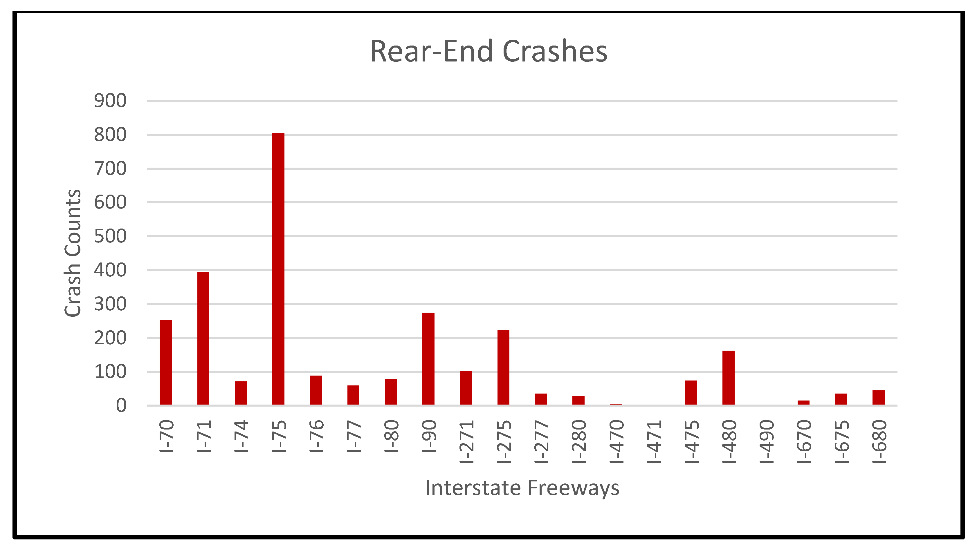
The data used in this study were obtained from the Highway Safety Information System (HSIS). These data pertain to 2021 and focus on interstate freeways 1 in the state of Ohio (see Figure 1). Some freeways serve as either ring freeways around major cities in Ohio or as connectors to other major freeways. Additionally, still other freeways function as major interstates connecting Ohio with other states. The data were received in three Excel files: a segment file, crash data, and a curve file. The segment file contains homogeneous segments, the crash data provide information about each crash, and the curve file contains details about horizontal curves. Rear-end crashes were extracted from the crash data file and then merged with the segment file using mileposts that marked the start and end of each segment. Similarly, the curve file was merged with the segment file to determine whether each segment was curved or not. The county population data were downloaded from The United States Census Bureau’s website (data.census.gov) and merged with the segment file based on county names. The final dataset comprises 1833 homogeneous segments that included 2745 recorded rear-end crashes on 20 interstate freeways extending over approximately 1313 miles (see Figure 2). These freeways exhibit variations in terms of rear-end crashes, as depicted in Figure 3.

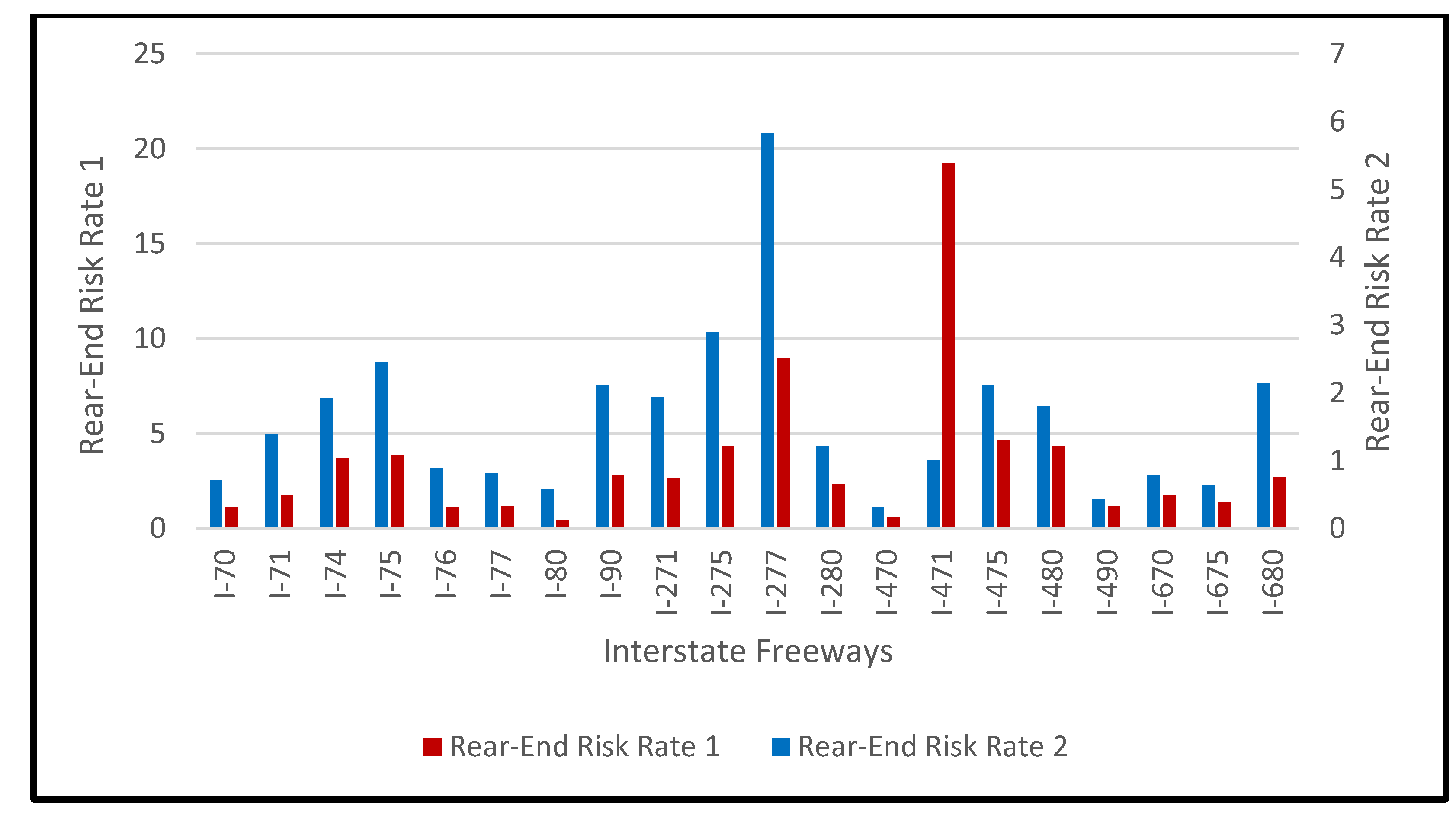
Figure 3 shows that some interstate freeways experience more rear-end crashes than others. For example, Interstate Freeway I-75 experiences around 800 rear-end crashes. Consequently, the expected rear-end crash counts for segments located on interstate freeways with a high frequency of rear-end crashes differ significantly from those on interstate freeways with low frequencies. To account for this heterogeneity across interstate freeways, the study computed two ratings. Risk Rate 1 is calculated as the total number of rear-end crashes divided by the total distance in miles on a particular interstate freeway. Risk Rate 2, on the other hand, is calculated as the total number of rear-end crashes divided by the total number of segments in that same interstate freeway. Risk Rate 2 is preferred over Risk Rate 1 because it provides more realistic values. Risk Rate 1 tends to yield higher values as compared to Risk Rate 2, as depicted in Figure 4. Nevertheless, one of the two ratings should be selected that better accounts for the heterogeneity between interstate freeways. However, these interstate freeways extend through various counties. A grouping variable is created that groups segments that are located within the same interstate freeway and county. This group variable aims to account for unobserved heterogeneity across counties within the same interstate freeways. The summary statistics for the considered variables are shown in

Table 3. Summary statistics for the considered variables.

Variables	Mean	Range	SD
Rear-end crash counts	1.498	0–54	3.525
Ln (AADT) of passenger car	10.659	8.418–11.938	0.615
Ln (segment length) (miles)	−1.267	−6.908–2.520	1.539
Inner shoulder width (feet)	15.532	0–60	9.125
Outer shoulder width (feet)	20.679	0–40	3.366
Area indicator(0 for urban and 1 for rural)	0.267	0–1	0.443
Rear-end crash risk rate 1	2.310	0.408–19.231	1.427
Rear-end crash risk rate 2	1.498	0.308–5.833	0.788
Number of lanes	5.380	4–10	1.474
Curved segment indicator (0 for straight segments, 1 for curved segments)	0.014	0–1	0.116
Ln (county population)	12.467	10.273–14.091	1.141

. However, the inner or outer shoulder widths represent the sum of the widths of the left or right sides, respectively, for both directions.

2.2. Model Description

The negative binomial (NB) model is well suited to handling over-dispersion issues. Crash counts are often over-dispersed, meaning their variance exceeds their mean [31]. The NB model accounts for this by introducing a dispersion parameter, which is denoted as k based on the following relationship:

$${\sigma }^2=\mu +{\displaystyle \frac{{\mu }^2}{k}}$$

(1)

Here, ${\sigma }^2$ represents the variance and $\mu$ represents the mean. As the dispersion parameter approaches infinity, the last term in Equation (1) approaches zero, simplifying the relationship to variance equals mean. In such cases, the Poisson model becomes more appropriate than the NB model [31]. However, the expected crash counts per segment, which are denoted as µ_i, are expressed as a log-linear function of explanatory variables, as follows:

$${\mu }_i=\exp \left(B{\mathit{X}}_{\mathit{i}}+{\epsilon }_i\right)$$

(2)

In Equation (2), X_i represents a vector of explanatory variables, B corresponds to the estimated fixed coefficients, and ε_i represents the error term. The error term follows a gamma distribution with a mean of 1 and a variance of 1/k.

The negative binomial density function is given by [32]:

$$f\left(y_i;k,{\mu }_i\right)={\displaystyle \frac{\mathsf{\Gamma }\left(y_i+k\right)}{\mathsf{\Gamma }\left(\mathrm{k}\right)\times y_i!}}\times {\left({\displaystyle \frac{k}{{\mu }_i+k}}\right)}^k\times {\left({\displaystyle \frac{{\mu }_i}{{\mu }_i+k}}\right)}^{y_i}$$

(3)

In Equation (3), $\mathsf{\Gamma }\left(.\right)$ denotes the gamma function and y_i represents the crash counts per segment i. All other terms are defined in the text above.

In [24], the random parameters were allowed to vary across individual observations or segments. In this study, the random parameters are allowed to vary across groups of segments, as shown by Equation (4):

$${\mathit{B}}_{\mathit{i}}=\mathit{B}+{\mathit{U}}_{\mathit{g}} \mathsf{\forall } \mathit{i} \in group g$$

(4)

Here, B represents a vector of the mean estimated parameters for explanatory variables, X_i. U_g is a vector of the random deviations for group g. These deviations are assumed to follow a normal distribution, with a mean of zero and a standard deviation $\sigma$. These random parameters account for unobserved heterogeneity across groups [33]. However, the correlations between these random parameters are assumed to be zero. To allow for correlated parameters, Equation (4) should be rewritten as shown in Equation (5):

$${\mathit{B}}_{\mathit{i}}=\mathit{B}+\mathit{C}{\mathit{U}}_{\mathit{g}} \mathsf{\forall } \mathit{i} \in group g$$

(5)

where C is the variance–covariance matrix. Its diagonal elements are the variances of random parameters, and its off-diagonal elements represent the covariance between the random parameters. Because the random parameters are allowed to vary across groups, the model developed using the functional form in Equation (4) is referred to as an uncorrelated grouped random parameters model or a two-level model. The model developed using the functional form in Equation (5) is called a correlated grouped random parameters model or a correlated two-level model. All models are estimated using the Generalized Linear Mixed Models with Template Model Builder (glmmTMB) R package, which uses the maximum likelihood estimation and Laplace approximation to integrate over random parameters [34].

2.3. Evaluating Metrics

The likelihood ratio test (LRT) is employed to assess the significance of each explanatory variable in a model. A bottom-up approach is used to construct the models. The LRT test statistic, which evaluates competing models, is expressed as follows in Equation (6):

$${\chi }^2=devianc{e}_{Model 1}-devianc{e}_{Model 2}$$

(6)

Here, χ² represents the test statistic and follows a Chi-squared distribution, with the degrees of freedom equal to the difference in the number of estimated parameters between the two competing models. The term “$deviance$” corresponds to twice the negative log-likelihood value at convergence [32].

Additionally, the developed models, namely the fixed, two-level, and correlated two-level negative binomial models, are further evaluated using Akaike’s Information Criterion (AIC) and Schwarz’s Bayesian information criterion (BIC). These criteria incorporate penalties based on the estimated parameters and the number of observations, as shown in Equations (7) and (8) [35]:

$$AIC=deviance+2\times q$$

(7)

$$BIC=deviance+q\times \ln \left(N\right)$$

(8)

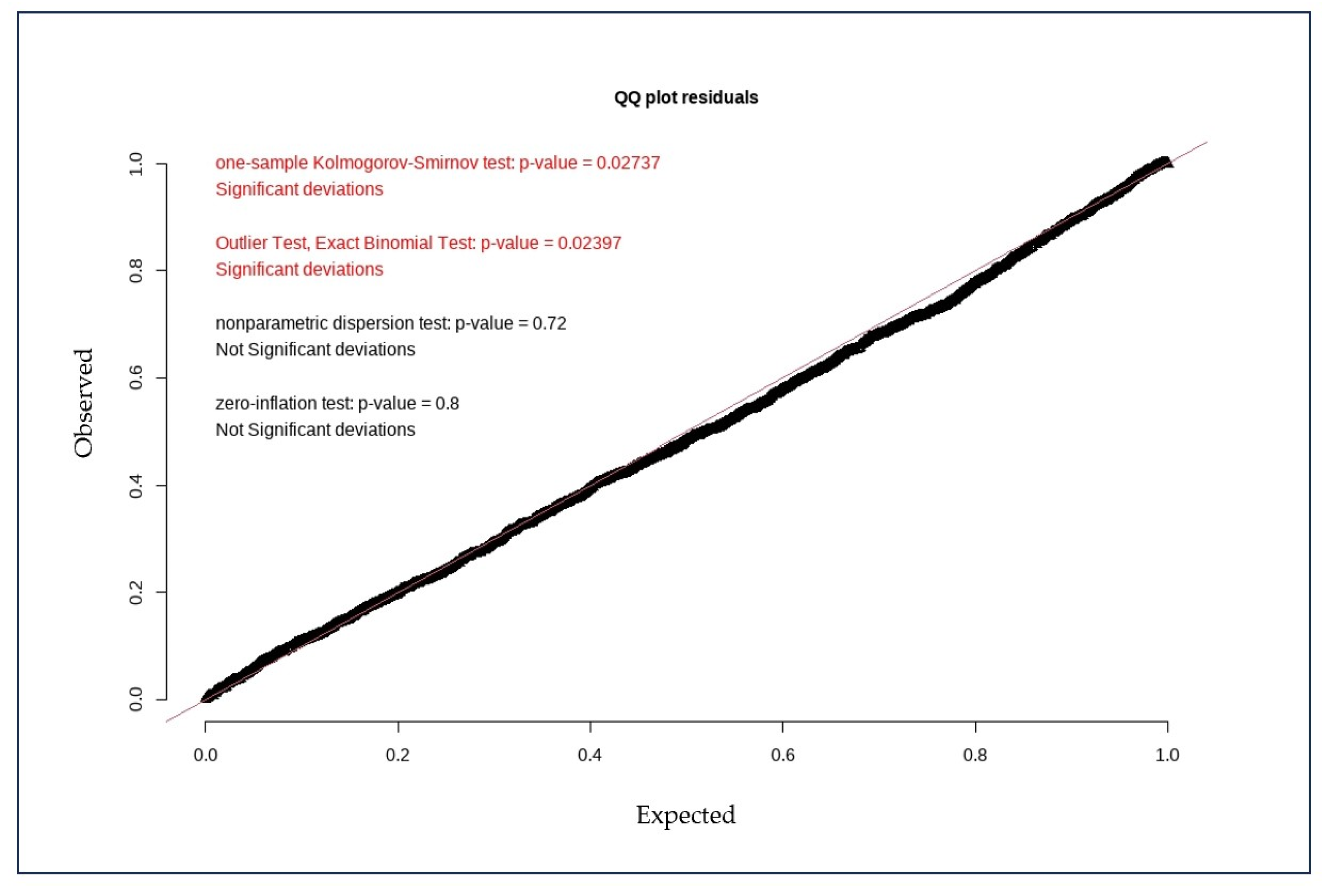
Here, q represents the number of estimated parameters, and N is the number of observations. All other terms are defined in the text above. Furthermore, residual diagnostics for the developed models are conducted using quantile–quantile (QQ) residual plots generated by the DHARMa R package [36]. In these plots, the x-axis represents the simulated residuals under the assumed distribution of the model, while the y-axis represents the observed distribution of the residuals. These plots are constructed for the three models mentioned above. Each plot includes four tests: a one-sample Kolmogorov–Smirnov (KS) test to assess the agreement between the distributions of observed and expected values, an outlier test to evaluate the alignment between outlier amounts and expectations, a dispersion test to compare simulated dispersion with observed dispersion, and a zero-inflation test to check for an excess of zeros in the data. Moreover, these plots and tests rely on 200 simulated values for each observation. The accuracy of each model is also evaluated using the root mean square error (RMSE) [37]. The RMSE can be computed via Equation (9):

$$RMSE=\sqrt{{\displaystyle \frac{{{\displaystyle \sum }}_{i=1}^N{\left(O{V}_i-F{V}_i\right)}^2}{N}}}$$

(9)

Here, OV stands for observed values and FV stands for fitted values. All other terms are defined above.

3. Study Results

Crash counts often show over-dispersion, where the variance surpasses the mean. For instance, Table 3 shows a mean rear-end crash count of 1.498 and a variance of 12.43 (SD: 3.525). This supports using the negative binomial model over the Poisson model. Additionally, excess zeros contribute to over-dispersion and heterogeneity. To address this, the intercept-only zero-inflated negative binomial model was compared with the intercept-only negative binomial model. Both models had a deviance of 5686.8, indicating that excess zeros did not significantly affect the results. All the explanatory variables in Table 3 were assessed individually to determine their contributions to model fit using LRT, as described in the methodology. Of the ten variables tested, six were found to be significant predictors of rear-end crashes: the natural logarithm of AADT, the natural logarithm of segment length, inner shoulder width, area, rear-end crash Risk Rate 1, and rear-end crash Risk Rate 2. Outer shoulder width, number of lanes, curved segment indicator, and county population were not statistically significant predictors. However, the model incorporating rear-end crash Risk Rate 2 demonstrates a superior fit compared to the model incorporating rear-end crash Risk Rate 1. Consequently, Risk Rate 2 is selected and will be referred to as the rear-end crash risk rate for the remainder of this manuscript. Interactions between significant variables were explored, with only one significant interaction being found, between area and rear-end crash rate. The significant variables substantially improved model fit, reducing the deviance value by approximately 1105. Then, each significant variable is allowed to vary across groups, and the model fit is tested using LRT. If the p-value is less than 0.05, the random parameter is retained in the model. Three parameters are found to randomly vary across groups: the intercept, the natural logarithm of segment length, and the inner shoulder width. Similarly, those random parameters are allowed to be correlated with one another. The only correlation that significantly improved the model fit is the correlation between the intercept and the inner shoulder width.

Table 4. Results of model estimations.

Model	Fixed Negative Binomial			Two-Level Negative Binomial			Correlated Two-Level Negative Binomial
Fixed Parameters	Estimate	Std. Error	Z-stat	Estimate	Std. Error	Z-stat	Estimate	Std. Error	Z-stat
Intercept	−14.613	0.814	−17.947	−14.813	1.056	−14.031	−14.477	1.053	−13.743
Ln (AADT)	1.410	0.078	18.182	1.420	0.101	14.075	1.387	0.101	13.740
Ln (Segment length) (LSL)	0.838	0.031	26.726	0.846	0.037	22.621	0.846	0.036	23.456
Inner shoulder width (ISR)	−0.021	0.004	−5.502	−0.020	0.005	−4.020	−0.021	0.006	−3.197
Area indicator	0.308	0.203	1.512	0.356	0.230	1.546	0.386	0.234	1.647
Rear-end crash risk rate (RECRR)	0.316	0.051	6.209	0.321	0.073	4.402	0.333	0.071	4.679
RECRR-Area indicator interaction	−0.449	0.134	−3.349	−0.424	0.149	−2.844	−0.453	0.152	−2.986
Random parameters
Standard deviation of intercept (Negative sign percentages)	-	-	-	0.279 ≈100%	0.053	5.290	0.555 ≈100%	0.097	5.703
Standard deviation of LSL (Negative sign percentages)	-	-	-	0.126 ≈0%	0.036	3.541	0.107 ≈0%	0.036	2.970
Standard deviation of ISR (Negative sign percentages)	-	-	-	0.009 98.7%	0.003	2.703	0.028 77.3%	0.006	4.460
Intercept-IRS Correlation	-			-			−0.88

shows the three models’ estimations. The coefficients of all variables in the three models have realistic and intuitive values. For example, the natural logarithms of AADT and segment length are aligned with those in prior studies [24,25]. The coefficient for inner shoulder width is negative, indicating that an increase in inner shoulder width is associated with a decrease in rear-end crashes. This finding is consistent with the results reported in [16], which suggest that the temporary use of the left shoulder is linked to a reduction in total crashes.

Table 4 also presents the estimates of the random parameters. As outlined in the model description section, these parameters are assumed to follow a normal distribution. For example, the coefficient of inner shoulder width is normally distributed with a mean of −0.021 and a standard deviation of 0.028 for the correlated two-level negative binomial model. This means that 77.3% of the coefficients are negative, indicating that an increase in inner shoulder width is associated with a decrease in rear-end crash counts.

Table 5. A comparison of three developed models.

Model	Fixed Negative Binomial	Two-Level Negative Binomial		Correlated Two-Level Negative Binomial
Goodness-of-fit measures
Deviance	4581.4	4556.1		4546.8
AIC	4597.4	4578.1		4570.8
BIC	4641.5	4638.8		4637
Degrees of freedom	8	11		12
Likelihood ratio test
Difference of degrees of freedom	3		1
Chi-square statistics	25.313		9.272
p-value	<0.0001		0.0023
Forecasting accuracy
RMSE	2.597	2.453		2.452

presents the comparison metrics for the three models. The correlated two-level negative binomial model consistently outperformed the others across all metrics, showing the lowest AIC and BIC values—at least 7 points lower in AIC and 1.5 points lower in BIC compared to the other models. This smaller reduction in BIC was expected due to its stricter penalty for additional parameters. The LRT was conducted between the fixed negative binomial model and the two-level negative binomial model. The test indicated that allowing the intercept, segment length, and inner shoulder width to vary across routes significantly improved the model fit, confirmed by a p-value less than 0.0001 as shown in Table 5. A further LRT between the correlated two-level negative binomial model and the two-level negative binomial model showed that allowing correlation between the intercept and inner shoulder width significantly improved the model fit, with a p-value of 0.0023 as shown in Table 5. Additionally, the correlated two-level negative binomial model had the lowest RMSE, indicating it was the best fit among the three models. Diagnostic plots (Figure 5, Figure 6 and Figure 7) support the correlated two-level negative binomial model, showing a QQ plot resembling a straight line and no significant deviations from model assumptions based on the outlined tests in the methodology (see Figure 7). In contrast, Figure 5 exhibits a QQ plot that appears to be a straight line but reveals significant deviations based on the KS and outlier tests. Similarly, Figure 6 shows a QQ plot resembling a straight line but indicating an excessive number of outliers.

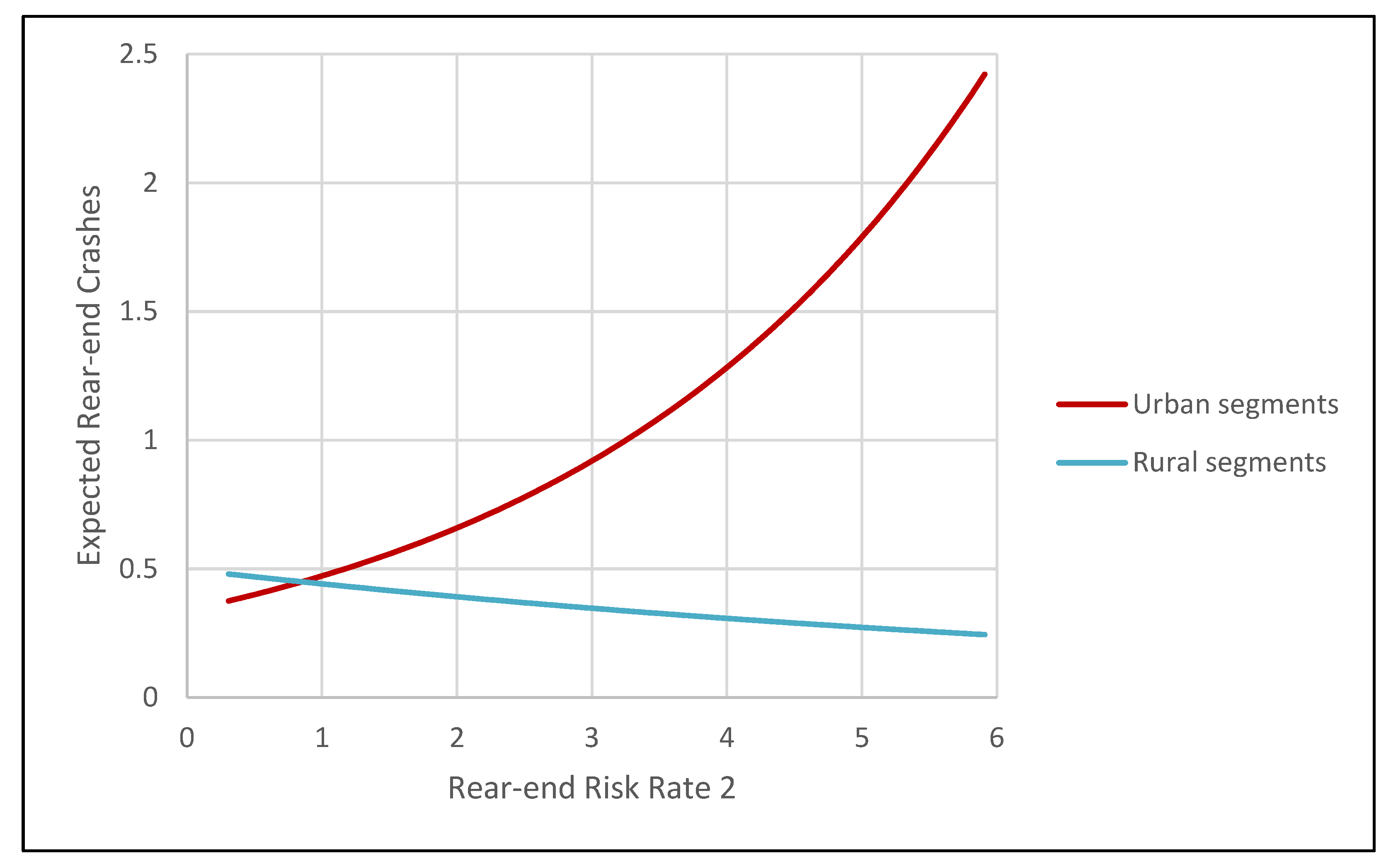
Given that the correlated two-level negative binomial model demonstrates a superior fit, it is advisable to visualize the significant interaction based on this model. Figure 8 illustrates the interaction between the rear-end crash risk rate and a segment’s location, either urban or rural. Interestingly, as the rear-end crash risk increases, the expected number of rear-end crashes also increases, but this effect is observed only in urban segments. Rural segments, on the other hand, exhibit minimal variation in expected rear-end crashes as the rear-end crash risk increases. This finding is aligned with a study conducted by [4], which reported that rear-end crashes are more frequent in urban areas and major cities. Meanwhile, this study concludes that rear-end crashes are more frequent in urban segments of interstate freeways with a high rear-end crash risk.

Table 6. Average marginal effects for the three models.

Variables	Fixed Negative Binomial	Two-Level Negative Binomial	Correlated Two-Level Negative Binomial
Ln (AADT)	2.120	2.099	2.0418
Ln (segment length)	1.259	1.252	1.2507
Inner shoulder width	−0.0318	−0.0288	−0.0318
Area indicator	−0.6049	−0.4996	−0.516
Rear-end crash risk rate	0.3885	0.395	0.406

presents the average marginal effects for each explanatory variable. Unit increases in the natural logarithms of AADT and segment length are associated with average increases in rear-end crashes of 2.04 and 1.25, respectively. Conversely, a one-foot increase in the inner shoulder width is expected to decrease the number of rear-end crashes by an average of 0.032, meaning there are 0.032 fewer crashes, on average, for each additional foot of shoulder width. On average, rural segments are predicted to have 0.5 fewer rear-end crashes than urban segments. Lastly, the rear-end crash risk rate, ranging from roughly 0.3 to 6, as shown in Table 3, helps address heterogeneity across interstate freeways. Notably, Table 6 reveals that a one-unit increase in this variable is associated with an average increase in rear-end crashes of 0.41. Thus, this proposed systematic approach clearly addresses the differences between interstate freeways by gauging the rear-end crash rate for each interstate freeway and employing random parameters that account for the heterogeneity between segments on the same stretch of interstate freeway but in different counties. A previous study [24] found that allowing parameters to vary across each observation improved the model fit, but allowing correlations between parameters did not. However, this study found that allowing parameters to vary across routes (segments in the same county) and allowing correlation between intercept and inner shoulder width significantly improved the model. This conclusion aligns with another previous study [1], which found that allowing parameters improved the model fit, though that study focused on crash severity. The unique contributions of this approach are that the effects of the natural logarithm of segment length and inner shoulder width vary across county routes, correlations between intercept and inner shoulder width are allowed, and rear-end crash risk rates between interstates are controlled. This approach explicitly specifies the dependency between observations and enhances model fit and accuracy. It can be directly applied to interstate freeways in the state of Ohio to identify problematic segments or to interstate freeways in other states or cities, with calibration as outlined in [13,14,17]. These findings underscore the need for targeted interventions to address the identified factors and reduce the frequency of rear-end crashes on interstate freeways.

4. Conclusions

This study analyzed rear-end crash counts on 20 interstate freeways in the state of Ohio. These 20 interstate freeways differ substantially in terms of rear-end crash counts. Thus, a new approach is proposed to account for this heterogeneity. The rear-end crash risk rate is calculated for each interstate freeway. This rear-end crash risk rate aims to account for heterogeneity across interstate freeways. Three models were developed: a standard negative binomial model, an uncorrelated two-level negative binomial model, and a correlated two-level negative binomial model. The study revealed that the correlated two-level negative binomial model outperformed the other two models. In the correlated two-level negative binomial model, the parameters are allowed to vary across groups, and significant random parameters are allowed to be correlated. These groups cluster the segments located in the same interstate freeway and county together. As compared to the other two models, this model provides better fit, prediction accuracy, and adherence to diagnostic plots and tests, indicating that dependency and heterogeneity among observations are being addressed. In other words, there are significant variations across interstate freeways, which are addressed by the rear-end crash risk rate, and there are significant variations across segments located in different counties but on the same interstate freeway, which are addressed by the correlated grouped random parameters. Also, the coefficients of all significant explanatory variables agree with those estimated in previous studies. Interestingly, rear-end crashes are expected to occur more frequently in urban segments of freeways with high rear-end risk rates. However, rural segments experience no such significant variations as a function of the rear-end crash risk rate. An increase in the inner shoulder width is associated with a decrease in expected rear-end crashes. This proposed systematic approach can be directly applied to interstate freeways in Ohio to identify problematic segments or adapted for use in other states or cities after calibration to local conditions. This approach integrates all interstate freeways into a single system while accounting for their heterogeneity. However, this approach is not without limitations. It predicts only rear-end crash counts, ignoring any potential correlation with other crash types. Future studies could develop a multivariate crash prediction model that accounts for correlations among crash types. Despite this limitation, it provides analysts and decision-makers with a clear understanding of the locations of problematic segments concerning rear-end crashes and the contributing variables.

References

1. Yuan, R.; Gu, X.; Peng, Z.; Xiang, Q. Exploring Differences in Injury Severity between Occupant Groups Involved in Fatal Rear-End Crashes: A Correlated Random Parameter Logit Model with Mean Heterogeneity. Transp. Lett. 2023. [Google Scholar] [CrossRef]
2. Dimitriou, L.; Stylianou, K.; Abdel-Aty, M.A. Assessing Rear-End Crash Potential in Urban Locations Based on Vehicle-by-Vehicle Interactions, Geometric Characteristics and Operational Conditions. Accid. Anal. Prev. 2018, 118, 221–235. [Google Scholar] [CrossRef]
3. Pešić, A.; Stephens, A.N.; Newnam, S.; Čičević, S.; Pešić, D.; Trifunović, A. Youth Perceptions and Attitudes towards Road Safety in Serbia. Systems 2022, 10, 191. [Google Scholar] [CrossRef]
4. Swain, R.; Larue, G.S. Looking Back in the Rearview: Insights into Queensland’s Rear-End Crashes. Traffic Inj. Prev. 2024, 25, 138–146. [Google Scholar] [CrossRef]
5. Chen, F.; Song, M.; Ma, X. Investigation on the Injury Severity of Drivers in Rear-End Collisions between Cars Using a Random Parameters Bivariate Ordered Probit Model. Int. J. Environ. Res. Public. Health 2019, 16, 2632. [Google Scholar] [CrossRef]
6. Shao, X.; Ma, X.; Chen, F.; Song, M.; Pan, X.; You, K. A Random Parameters Ordered Probit Analysis of Injury Severity in Truck Involved Rear-End Collisions. Int. J. Environ. Res. Public. Health 2020, 17, 395. [Google Scholar] [CrossRef] [PubMed]
7. Sharafeldin, M.; Farid, A.; Ksaibati, K. Injury Severity Analysis of Rear-End Crashes at Signalized Intersections. Sustainability 2022, 14, 13858. [Google Scholar] [CrossRef]
8. Wang, C.; Xia, Y.; Chen, F.; Cheng, J.; Wang, Z. Assessment of Two-Vehicle and Multi-Vehicle Freeway Rear-End Crashes in China: Accommodating Spatiotemporal Shifts. Int. J. Environ. Res. Public. Health 2022, 19, 10282. [Google Scholar] [CrossRef]
9. Wang, C.; Chen, F.; Zhang, Y.; Wang, S.; Yu, B.; Cheng, J. Temporal Stability of Factors Affecting Injury Severity in Rear-End and Non-Rear-End Crashes: A Random Parameter Approach with Heterogeneity in Means and Variances. Anal. Methods Accid. Res. 2022, 35, 100219. [Google Scholar] [CrossRef]
10. Zou, R.; Yang, H.; Yu, W.; Yu, H.; Chen, C.; Zhang, G.; Ma, D.T. Analyzing Driver Injury Severity in Two-Vehicle Rear-End Crashes Considering Leading-Following Configurations Based on Passenger Car and Light Truck Involvement. Accid. Anal. Prev. 2023, 193, 107298. [Google Scholar] [CrossRef]
11. Wang, C.; Chen, F.; Zhang, Y.; Cheng, J. Analysis of Injury Severity in Rear-End Crashes on an Expressway Involving Different Types of Vehicles Using Random-Parameters Logit Models with Heterogeneity in Means and Variances. Transp. Lett. 2023, 15, 742–753. [Google Scholar] [CrossRef]
12. HSM Highway Safety Manual; American Association of State Highway and Transportation Officials: Washington, DC, USA, 2010.
13. Administration, F.H. Crash Prediction Module. Available online: https://highways.dot.gov/research/interactive-highway-safety-design-model/modules/crash-prediction-module (accessed on 11 September 2024).
14. Al-Ahmadi, H.M.; Jamal, A.; Ahmed, T.; Rahman, M.T.; Reza, I.; Farooq, D. Calibrating the Highway Safety Manual Predictive Models for Multilane Rural Highway Segments in Saudi Arabia. Arab. J. Sci. Eng. 2021, 46, 11471–11485. [Google Scholar] [CrossRef]
15. Erieba, O.; Pappalardo, G.; Hassan, A.; Said, D.; Cafiso, S. Assessment of the Transferability of European Road Safety Inspection Procedures and Risk Index Model to Egypt. Ain Shams Eng. J. 2024, 15, 102502. [Google Scholar] [CrossRef]
16. Hasan, T.; Abdel-Aty, M. Short-Term Safety Performance Functions by Random Parameters Negative Binomial-Lindley Model for Part-Time Shoulder Use. Accid. Anal. Prev. 2024, 199, 107498. [Google Scholar] [CrossRef] [PubMed]
17. National Academies of Sciences, Engineering and Medicine. Improved Prediction Models for Crash Types and Crash Severities; The National Academies Press: Washington, DC, USA, 2021. [CrossRef]
18. Anastasopoulos, P.C.; Mannering, F.L. A Note on Modeling Vehicle Accident Frequencies with Random-Parameters Count Models. Accid. Anal. Prev. 2009, 41, 153–159. [Google Scholar] [CrossRef]
19. Sawalha, Z.; Sayed, T. Traffic Accident Modeling: Some Statistical Issues. Can. J. Civ. Eng. 2006, 33, 1115–1124. [Google Scholar] [CrossRef]
20. Choudhary, A.; Garg, R.D.; Jain, S.S. Safety Impact of Highway Geometrics and Pavement Parameters on Crashes along Mountainous Roads. Transp. Eng. 2024, 15, 100224. [Google Scholar] [CrossRef]
21. Mannering, F.L.; Bhat, C.R. Analytic Methods in Accident Research: Methodological Frontier and Future Directions. Anal. Methods Accid. Res. 2014, 1, 1–22. [Google Scholar] [CrossRef]
22. Champahom, T.; Se, C.; Jomnonkwao, S.; Kasemsri, R.; Ratanavaraha, V. Analysis of the Effects of Highway Geometric Design Features on the Frequency of Truck-Involved Rear-End Crashes Using the Random Effect Zero-Inflated Negative Binomial Regression Model. Safety 2023, 9, 76. [Google Scholar] [CrossRef]
23. Bisht, L.S.; Tiwari, G. Assessment of Fatal Rear-End Crash Risk Factors of an Expressway in India: A Random Parameter NB Modeling Approach. J. Transp. Eng. A Syst. 2023, 149, 04022111. [Google Scholar] [CrossRef]
24. Saeed, T.U.; Hall, T.; Baroud, H.; Volovski, M.J. Analyzing Road Crash Frequencies with Uncorrelated and Correlated Random-Parameters Count Models: An Empirical Assessment of Multilane Highways. Anal. Methods Accid. Res. 2019, 23, 100101. [Google Scholar] [CrossRef]
25. Almutairi, O. A Nested Grouped Random Parameter Negative Binomial Model for Modeling Segment-Level Crash Counts. Heliyon 2024, 10, e28900. [Google Scholar] [CrossRef] [PubMed]
26. Venkataraman, N.S.; Ulfarsson, G.F.; Shankar, V.; Oh, J.; Park, M. Model of Relationship between Interstate Crash Occurrence and Geometrics: Exploratory Insights from Random Parameter Negative Binomial Approach. Transp. Res. Rec. 2011, 2236, 41–48. [Google Scholar] [CrossRef]
27. Yan, Y.; Zhang, Y.; Yang, X.; Hu, J.; Tang, J.; Guo, Z. Crash Prediction Based on Random Effect Negative Binomial Model Considering Data Heterogeneity. Phys. A Stat. Mech. Its Appl. 2020, 547, 123858. [Google Scholar] [CrossRef]
28. Champahom, T.; Jomnonkwao, S.; Karoonsoontawong, A.; Ratanavaraha, V. Spatial Zero-Inflated Negative Binomial Regression Models: Application for Estimating Frequencies of Rear-End Crashes on Thai Highways. J. Transp. Saf. Secur. 2022, 14, 523–540. [Google Scholar] [CrossRef]
29. Islam, A.S.M.M.; Shirazi, M.; Lord, D. Grouped Random Parameters Negative Binomial-Lindley for Accounting Unobserved Heterogeneity in Crash Data with Preponderant Zero Observations. Anal. Methods Accid. Res. 2023, 37, 100255. [Google Scholar] [CrossRef]
30. Wang, W.; Yang, Y.; Yang, X.; Gayah, V.V.; Wang, Y.; Tang, J.; Yuan, Z. A Negative Binomial Lindley Approach Considering Spatiotemporal Effects for Modeling Traffic Crash Frequency with Excess Zeros. Accid. Anal. Prev. 2024, 207, 107741. [Google Scholar] [CrossRef]
31. Hilbe, J.M. Negative Binomial Regression; Cambridge University Press: Cambridge, UK, 2007. [Google Scholar]
32. Zuur, A.F.; Ieno, E.N.; Walker, N.J.; Saveliev, A.A.; Smith, G.M. Mixed Effects Models and Extensions in Ecology with R; Springer: Berlin/Heidelberg, Germany, 2009; Volume 574. [Google Scholar]
33. Mannering, F.L.; Shankar, V.; Bhat, C.R. Unobserved Heterogeneity and the Statistical Analysis of Highway Accident Data. Anal. Methods Accid. Res. 2016, 11, 1–16. [Google Scholar] [CrossRef]
34. Brooks, M.E.; Kristensen, K.; van Benthem, K.J.; Magnusson, A.; Berg, C.W.; Nielsen, A.; Skaug, H.J.; Mächler, M.; Bolker, B.M. GlmmTMB Balances Speed and Flexibility among Packages for Zero-Inflated Generalized Linear Mixed Modeling. R J. 2017, 9, 378–400. [Google Scholar] [CrossRef]
35. Zhang, H.; Yao, X.; Seong, J.T.; Alshanbari, H.M.; Albalawi, O. A New Weighted Probabilistic Model for Analyzing the Injury Rate in Public Transport Road Accidents. Alex. Eng. J. 2024, 101, 147–157. [Google Scholar] [CrossRef]
36. Hartig, F. DHARMa: Residual Diagnostics for Hierarchical (Multi-Level/Mixed) Regression Models; R Packag Version 020 2018.
37. Aljuaydi, F.; Wiwatanapataphee, B.; Wu, Y.H. Multivariate Machine Learning-Based Prediction Models of Freeway Traffic Flow under Non-Recurrent Events. Alex. Eng. J. 2023, 65, 151–162. [Google Scholar] [CrossRef]
Figure 1. A map of Ohio’s considered interstate freeways.
Systems 12 00438 g001
Figure 2. Data on Ohio freeways.
Systems 12 00438 g002
Figure 3. Rear-end crashes for each interstate freeway.
Systems 12 00438 g003
Figure 4. Rear-end crash risk rating for each freeway.
Systems 12 00438 g004
Figure 5. Quantile–quantile residuals plot for fixed parameter negative binomial model.
Systems 12 00438 g005
Figure 6. Quantile–quantile residuals plot for two-level negative binomial model.
Systems 12 00438 g006
Figure 7. Quantile–quantile residuals plot for correlated two-level negative binomial model.
Systems 12 00438 g007
Figure 8. The interaction between rear-end risk rate and area.
Systems 12 00438 g008