Investigation of Traffic System with Traffic Restriction Scheme in the Presence of Automated and Human-Driven Vehicles

Abstract

In the context of transportation development, the simultaneous emergence of automated vehicles (AVs) and human-driven vehicles (HDVs) can lead to varied traffic system performance. For the purpose of improving traffic systems, this paper proposes a traffic restriction scheme only for HDVs. We develop a variational inequality (VI) model to describe travel mode and route choices under this restriction scheme and design an algorithm to solve the model. The proposed model and algorithm are applied to a Sioux Falls network example to evaluate the effects of the traffic restriction scheme. Our findings indicate that the scheme improves overall social welfare, with a higher proportion of restricted travelers leading to greater social welfare as well as increased travel demand due to changes in capacity. However, some lower exogenous monetary factors lead to negative social welfare, as the presence of AVs may exacerbate road congestion. Additionally, advancements in technology are needed to adjust the weightings of travel time and congestion level estimates to further enhance social welfare. These results offer valuable insights for traffic demand management in traffic systems with a mix of AVs and HDVs.

1. Introduction

Traffic restriction schemes have been implemented in various cities, such as Beijing, Bogotá, and Athens, with the primary objectives of alleviating congestion, reducing emissions, and achieving significant positive outcomes [1]. The specific implementation details of these schemes vary across different urban contexts. For example, in Beijing and Mexico City, vehicle access to restricted areas is regulated based on license plate numbers, employing systems such as the odd–even rule or the last-digit principle. In New York City, restrictions are placed on commercial delivery vehicles, preventing them from entering certain parts of Manhattan during designated times to mitigate congestion. Additionally, some cities have designed their restricted areas to prohibit the entry of high-emission vehicles. Consequently, traffic restriction schemes are widely recognized as effective measures for managing traffic demand.

Previous studies have examined traffic restriction schemes from various perspectives. Given the restriction scheme, Han et al. (2010) analyzed the efficiency of plate number-based rationing schemes within the context of system cost reduction [2]. Wang et al. (2010) investigated the effects of these restriction schemes in both short-term and long-term scenarios [3]. Regarding the optimization of such schemes, Shi et al. (2014) simultaneously designed the optimal restriction area and proportion to maximize social welfare while minimizing congestion levels [1]. Chen (2020) further optimized traffic restriction schemes by determining the optimal restricted plate numbers, considering the spatial distribution of vehicles [4]. Daganzo and Garcia (2000) proposed a hybrid scheme combining road pricing and rationing, which was subsequently applied to the San Francisco Bay Bridge by Nakamura and Kockelman (2002) [5,6]. Additionally, extensions of these schemes have been explored, including the integration of rationing with congestion pricing or the park-and-ride model [7,8]. However, Nie (2017) highlighted drawbacks of traffic restriction policies, particularly when considering the monetary costs associated with vehicle ownership [9].

The current traffic restriction strategies primarily focus on human-driven vehicles (HDVs). However, the integration of automated vehicles (AVs) into the traffic system offers the potential for significant improvements. Equipped with advanced sensors such as cameras, radar, and ultrasonic devices, AVs can accurately perceive their surroundings. These data are processed in real time by sophisticated AI algorithms, enabling AVs to make informed driving decisions that enhance the overall organization of the traffic system. As a result, AVs contribute to a reduction in traffic accidents by providing faster response times and maintaining consistent awareness of traffic conditions. Additionally, the optimized traffic flows facilitated by AVs can increase road capacity, improve travel speeds, and reduce both traffic congestion and vehicle emissions. The presence of AVs introduces changes to the traffic system, as they can be managed more efficiently than HDVs through technologies such as intelligent communication and automatic control. To be specific, the headways between vehicles may decrease when AVs follow other vehicles, leading to a redistribution of traffic flows in mixed AV and HDV environments [10]. This in turn alters the marginal costs for travelers compared to traditional traffic systems. Additionally, the criteria that influence travelers’ choices of transportation modes and routes may shift. AV passengers can engage in work or entertainment activities during their journeys, which may increase their tolerance for traffic congestion. Consequently, they might select different modes or routes, leading to changes in the overall performance of the traffic system. These developments may redetermine traffic restriction schemes. However, due to the ongoing development and refinement of the necessary technologies, the widespread adoption of AVs remains limited. Currently, the traffic system is characterized by a mix of HDVs and an increasing number of AVs. Therefore, it is significant to explore traffic restriction in a mixed traffic system in the presence of AVs and HDVs.

Plenty of studies pay attention to the capacity, stability of traffic flow, emissions reduction, and traffic safety in the whole traffic system involving AVs. The results show that connected automated vehicles (CAVs), which are able to communicate with other CAVs with equipment as a type of AV, are beneficial for the four aspects above on road segments to a large extent [11,12,13]. However, if CAVs are not able to communicate with front vehicles well, the stability worsens [14]. Several studies investigate impacts of congestion pricing on traffic systems in the presence of AVs, or AVs and shared automated vehicles (SAVs). Since AVs are rarely used in daily travel in reality, the studies adopted simulations to detect the effects, including performances of the traffic network in Austin and Berlin [15,16,17,18]. The results show the superiorities of congestion pricing when AVs, or AVs and SAVs, exist. Meanwhile, some studies establish mathematical models involving equilibrium and the optimal toll pattern to describe the traffic system, taking into consideration congestion pricing and AVs [19,20,21,22]. However, the congestion pricing based on the Pigouvian principle is not always valid, since the marginal trip costs are not strictly increasing [23]. Some pricing schemes are designed for optimal traffic systems such as the pricing scheme only applying to human-driven vehicles [20] and the pricing scheme involving SAVs [18].

To the best of our knowledge, few studies have explicitly examined multi-user traffic systems involving both AVs and HDVs, particularly in relation to congestion tolerance on road segments with traffic restriction schemes. Moreover, the impacts of traffic restriction schemes on such mixed-user traffic systems remain largely unexplored. Motivated by this gap, this paper aims to investigate the impacts of a traffic restriction scheme on a general network with mixed AV and HDV users. Our analysis considers the unique characteristics of AVs, such as their influence on road capacity, as well as the tolerance levels of travelers when selecting modes and routes.

The rest of this paper is organized as follows: Section 2 describes the traffic restriction scheme and presents the formula to describe the user equilibrium on a general network with the scheme. Section 3 provides the algorithm for the formula to capture the demand and flow patterns under the traffic restriction scheme. The model and algorithm are applied to numerical examples in Section 4, and Section 5 concludes the paper.

2. Traffic Restriction Scheme and Formulations for Travel Mode and Path Choices

2.1. Traffic Restriction Scheme

Traffic restrictions can potentially benefit the overall transportation system. Leveraging advanced technologies, automated vehicles (AVs) can reduce headways and thus increase road capacities. Consequently, a higher proportion of AVs could contribute to reduced congestion within the network. To enhance the effectiveness of the traffic system, we propose a cordon-based traffic restriction scheme for HDVs, where a proportion of human-driven vehicles (HDVs) are prohibited from entering a designated zone, while AVs face no such restrictions. The restricted cordon-based area consists of some connected links of the network, implying that the links constitute a unit part of the whole network. Travelers who are barred from entering the restricted area must either switch to an alternative mode of transportation or cancel their trips if they have no alternative path. For simplicity, we make the following assumptions:

Assumption 1.

There are three travel modes, AVs, HDVs, and transit.

Assumption 2.

Each traveler can afford at most one vehicle. This is realistic, particularly in developing countries where lower-income individuals may be prevalent.

Assumption 3.

Travel time by transit is constant, which is the common case for services such as subways or buses with dedicated lanes. For simplicity, we adopt this assumption in our analysis.

Given these assumptions, HDV travelers restricted from entering the designated area must either alter their routes or switch to a different mode if they choose to travel. In the absence of alternative routes, switching to another mode becomes necessary. Typically, traffic restrictions are enforced for one day at a time, meaning travelers only need to avoid using HDVs on those days. Consequently, purchasing an additional AV is not necessary. Thus, transit is the only feasible alternative mode of travel for those barred from the area. In reality, the cordon-based restriction scheme is widely used, since it is convenient to implement, which is the reason why we adopt the cordon-based restriction scheme in this paper.

2.2. Preliminaries and Constraints for the Model

Consider a general traffic network $(G,A)$, where $G$ is the set of nodes and $A$ is the set of the links on the network. Let $W, P$, and $M$ be the set of origin–destination (OD) pairs, the set of paths on the network, and the set of travel modes, respectively. The OD pair $w\in W$, the $p\in P$, and $m\in M=\{AV,HDV,Tr\}$ are also considered, where $AV$ represents automated vehicles, $HDV$ denotes human-driven vehicles, and $Tr$ means transit. There exists potential travel demand $\overline{d_w}$ between the OD pair $w$. The actual travel demand $d_w$ between this OD pair is determined by the minimal generalized travel cost ${\mu }_w$ between this OD pair, which is given by

$$d_w=\overline{d_w}\cdot \exp (-k{\mu }_w), w\in W$$

(1)

where $k$ is the sensitive parameter of the demand to the generalized travel cost. ${\mu }_w$ is the generalized minimal travel cost between the OD pair $w$. We use $d_w^{AV}$ to represent the demand traveling with automated vehicles between the OD pair $w$, $d_w^{HDV}$ to denote the demand traveling with human-driven vehicles between the OD pair $w$, and $d_w^{Tr}$ to denote the demand of travelers using transit on the network. Obviously, we have

$$d_w=d_w^{AV}+d_w^{HDV}+d_w^{Tr}, w\in W$$

(2)

Then, the travelers choose their paths for trips. $f_{w,p}^m$ denotes the flow of travel mode $m$ on path $p$ between the OD pair $w$. The travel demand and flow satisfy the relationship

$${\displaystyle \sum _{p\in P}{f}_{w,p}^m}=d_w^m, w\in W$$

(3)

In addition, the vehicle flow on link $a$ is given by

$$x_a={\displaystyle \sum _{w\in W}{\displaystyle \sum _{m\in \overline{M}}{\displaystyle \sum _{p\in P}{f}_{w,p}^m\cdot {\delta }_{ap}^w}}}, a\in A, \overline{M}=\{AV,HDV\}$$

(4)

And the vehicle flow of mode $\overline{m}$ on link $a$ can be expressed as

$$x_a^{\overline{m}}={\displaystyle \sum _{w\in W}{\displaystyle \sum _{p\in P}{f}_{w,p}^{\overline{m}}\cdot {\delta }_{ap}^w}}, a\in A$$

(5)

where ${\delta }_{ap}^w$ is a binary variable indicating that if path $p$ between the OD pair $w$ includes link $a$, it equals 1, and 0 otherwise. Note that according to assumption 3, there exist dedicated lines for transit; thus, the transit flows are not included in the flows on the road network.

2.3. Generalized Travel Cost Functions

Travelers decide their mode and path based on their travel cost, which is associated with flows and capacities on links. Note that the capacity of link $a$ in the presence of AVs is different from that in the absence of AVs. When AVs and HDVs operate on a link, there exist four car-following modes, AV–AV, AV–HDV, HDV–AV, and HDV–HDV, in which HDV–AV means an HDV follows an AV, and vice versa. There are various headways due to the mode, which are denoted by $T_a^{AA}$, $T_a^{AH}$, $T_a^{HA}$, and $T_a^{HH}$, respectively. Obviously, $T_a^{HA}=T_a^{HH}$, since the human-driven vehicles are operated by human beings. The technologies of AVs determine $T_a^{AH}$. Namely, a perfect connection of the AV and the HDV leads to less $T_a^{AH}$. Let $T_a^{HA}=T_a^{HH}=T_a^H$. Assuming the proportion of AVs and HDVs on link $a$ are $p_r^{a,AV}$ and $p_r^{a,HDV}$, respectively, the average headway on this link is expressed as

$$T_a=p_r^{a,AV}{p}_r^{a,AV}{T}_a^{AA}+p_r^{a,AV}{p}_r^{a,HDV}{T}_a^{AH}+p_r^{a,HDV}{T}_a^{HH}, a\in A$$

(6)

In Equation (6), the proportions $p_r^{a,AV}$ and $p_r^{a,HDV}$ imply the probability of the headways. For example, the headway between two AVs exists with the probability of two AVs traveling simultaneously, which leads to the first term of Equation (6). The other cases are $p_r^{a,AV}{p}_r^{a,HDV}{T}_a^{AH}$, $p_r^{a,HDV}{p}_r^{a,AV}{T}_a^{HA}$, and $p_r^{a,HDV}{p}_r^{a,HDV}{T}_a^{HH}$. Taking the sum of all the cases, we can obtain Equation (6), noting that $T_a^{HA}=T_a^{HH}$ and $p_r^{a,AV}+p_r^{a,HDV}=1$.

The capacity on link $a$ is calculated by

$$C_a={\displaystyle \frac{1}{T_a}}, a\in A$$

(7)

Equation (7) means each vehicle has the average $T_a$ in a unit hour, in which $T_a$ is measured by hours. Then, in the unit time, there are ${\displaystyle \frac{1}{T_a}}$ vehicles passing through link $a$, which represents the capacity.

If the technologies on the AV achieve the required level, $T_a^{AA}$ and $T_a^{AH}$ may be smaller than $T_a^{HA}$ and $T_a^{HH}$, respectively, resulting in more vehicles on the link, leading to a larger capacity. If not, they might be equal or even larger. Therefore, the capacity is relevant to the proportion of AVs and HDVs, as well as the technology level.

Travelers estimate the travel cost according to the travel time and the congestion level. A traveler might prefer the path with a comparatively long travel time and less congestion instead of the path with a shorter travel time and a comparatively higher congestion level. In this paper, we use the ratio of the link flow to the capacity, ${\displaystyle \frac{x_a}{C_a}}$, to denote the congestion level on link $a$. When a traveler drives an AV, they can proceed with things that they prefer and obtain in-vehicle utility, while an HDV driver has to focus on driving. We use $u[t_a(x_a,C_a)]$ to express the utility, which is associated with the travel time on link $a$. Then, the generalized link travel cost functions of an AV traveler and an HDV traveler on link $a$ is, respectively, given by

$$c_a^{AV}={\alpha }^{AV}{\lambda }_t{t}_a(x_a,C_a)+(1-{\alpha }^{AV})\gamma ({\displaystyle \frac{x_a}{C_a}})-\sigma u[t_a(x_a,C_a)], a\in A$$

(8)

$$c_a^{HDV}={\alpha }^{HDV}{\lambda }_t{t}_a(x_a,C_a)+(1-{\alpha }^{HDV})\gamma ({\displaystyle \frac{x_a}{C_a}}), a\in A$$

(9)

where ${\alpha }^{\overline{m}}$ is the weight that a traveler with mode $m$ focuses on the travel time, in which $0\le {\alpha }^{\overline{m}}\le 1$. Apparently, $1-{\alpha }^{\overline{m}}$ is the weight that a traveler with mode $\overline{m}$ focuses on the congestion level. Due to the utility of AV travelers, the weights are supposed to be different for each mode. The weights reflect the average level of a traffic system. If the travelers with AVs concentrate on travel time more, the value of ${\alpha }^{AV}$ is higher, and vice versa. ${\lambda }_t, \gamma , \sigma$ are the parameters to transfer travel time, congestion level, and in-vehicle utility into monetary cost. Actually, the parameter ${\lambda }_t$ is the value of time, which can be identified by the income and the working hours of the individual. The parameter $\gamma$ is psychological, indicating the travelers’ feelings about the unit congestion level, which can be identified by the revealed preference (RP) investigation (mainly by questionnaires) and analysis. The parameter $\sigma$, which is relevant to the willingness and in-vehicle activities of the travelers, denotes the unit in-vehicle utility implying the value of the things that the travelers do in the vehicle, and can be obtained by the RP investigation as well. Note that in the process, we collect the sample data from the population and then obtain the aggregated values of the parameters reflecting the whole population level through statistical approaches. Thus, the parameters, ${\alpha }^{\overline{m}}, {\lambda }_t, \gamma , \sigma$ can be regarded as the average reflection of all travelers. Since our model would be aggregated, using the values of the parameters is appropriate to explore the real performance without valid perturbation.

The generalized path travel cost for each type of traveler mode $\overline{m}$ is expressed as

$$c_{w,p}^{\overline{m}}={\varphi }^{\overline{m}}+{\displaystyle \sum _a{c}_a^{\overline{m}}\cdot {\delta }_{ap}^w}, w\in W, p\in P, \overline{m}\in M, a\in A$$

(10)

where ${\varphi }^{\overline{m}}$ is the amortized cost of owning a vehicle of mode $\overline{m}$. The path travel time with transit mode is calculated by

$$c_{w,p}^{Tr}=\tau +{\varphi }^{Tr}+{\displaystyle \sum _{a\in A}{\phi }^{Tr}\cdot t_a^0\cdot {\delta }_{ap}^w}, w\in W, p\in P$$

(11)

where ${\phi }^{Tr}$ is the coefficient and ${\varphi }^{Tr}$ is the discomfort of taking transit in a unit time, which is psychological and widely identified, and transferred to monetary cost by a questionnaire investigation. The ticket price for transit is denoted by $\tau$. The parameter $t_a^0$ is the free-flow travel time on link $a$, which indicates the travel time of a vehicle when no other vehicle is on this link, obtained by traffic investigation.

Let ${\mu }_w^m$ denote the minimal generalized travel cost of mode $m$ between the OD pair $w$. It is worth noticing that the traffic restriction scheme has no direct impact on AVs and transit, and the restricted travelers with HDVs choose alternative paths between some OD pairs and choose another mode between some other OD pairs since there is no alternative path. Denote $W^r$ as the set of OD pairs between which there is no alternative paths for restricted HDV travelers and $W/W^r$ as the set of OD pairs between which there exists at least one alternative path for them. Denote $\eta$ as the proportion of HDV travelers who are prohibited from entering the restricted area. Due to the sole choice of transit for them, the minimal generalized travel cost for the travelers with HDVs between OD pair $W^r$ is given by

$${\mu }_w^{HDV}=\eta {\mu }_w^{HDV,u}+(1-\eta ){\mu }_w^{Tr}, w\in W^r$$

(12)

where ${\mu }_w^{HDV,u}$ is the minimal generalized travel cost of unrestricted travelers using HDVs. On the contrary, the minimal generalized travel cost for the travelers with HDVs between the OD pair $W/W^r$ is expressed by

$${\mu }_w^{HDV}=\eta {\mu }_w^{HDV,u}+(1-\eta ){\mu }_w^{HDV,r}, w\in W/W^r$$

(13)

where ${\mu }_w^{HDV,r}$ is the minimal generalized travel cost of the restricted travelers using HDVs. Obviously, ${\mu }_w^{HDV,r}$$w\in W/W^r$.

2.4. Travel Mode Split

In this paper, we use the logit method to split the travel mode. However, the restricted travelers with HDVs between the OD pair $w\in W^r$ have to choose transit. Then, the demand for each mode is calculated by

$$d_w^m=d_w\cdot p_r^{w,m}, w\in W, m\in M$$

(14)

where $p_r^{w,m}$ is the probability of the travelers choosing mode $m$ between the OD pair $w$, which is calculated by

$$p_r^{w,m}={\displaystyle \frac{\exp (-\theta {\mu }_w^m)}{{\displaystyle \sum _{m\in M}\exp (-\theta {\mu }_w^m)}}}, w\in W, m\in M$$

(15)

where ${\mu }_w^m$ is the minimal generalized travel cost of mode $m$ between the OD pair $w$. Note that the restricted travelers using HDVs without the alternative path have to choose the transit mode to travel. In other words, the actual demand of transit between the OD pair $w\in W^r$ is computed by

$$d_w^{Tr,a}=d_w^{Tr}+\eta d_w^{HDV,r}, w\in W^r$$

(16)

The relationships among the demands are illustrated in Figure 1.

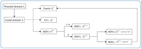
Figure 1. The relationships among the demands.

2.5. Mixed-User Equilibrium

After determining travel modes, travelers decide the paths they would take. It is widely assumed that all travelers follow the user equilibrium (UE) principle for the path choices. To be specific, the travelers of each mode between each OD pair choose the paths with the same and minimal path cost for this type of traveler, and no one can reduce the cost by changing his/her path. The following conditions describe the equilibrium:

$$c_{w,p}^i={\mu }_w^i\mathrm{if} f_{w,p}^{m^{\prime }}>0, w\in W, p\in P, i\in M^{\prime }$$

(17)

$$c_{w,p}^i\ge 0\mathrm{if} f_{w,p}^i=0, w\in W, p\in P, i\in M^{\prime }$$

(18)

$$c_{w,p}^{HDV,r}={\mu }_w^{HDV,r}\mathrm{if} f_{w,p}^{HDV,r}>0, w\in W^r, p\in P$$

(19)

$$c_{w,p}^{HDV,r}\ge {\mu }_w^{HDV,r}\mathrm{if} f_{w,p}^{HDV,r}=0, w\in W^r, p\in P$$

(20)

$M^{\prime }=\{AV,(HDV,u)\}$ and $(HDV,u)$ represent the HDV travelers who are not restricted to travel. Equations (17)–(20) demonstrate that if there exist travelers of mode $i$ or $HDV,r$ on path $p$ between their OD pair $w$, they experience the same minimal generalized travel cost. If no travelers of mode $i$ or $HDV,r$ are on the path, the generalized travel cost on this path is not smaller than that of this mode on the path utilized by the travelers. This is in accord with the UE condition mixed with AVs and HDVs. Note that the travel cost with transit is constant, which means all the travelers using transit can choose the shortest path and experience the same minimal generalized cost. Therefore, we assign all the transit travelers onto the shortest path without the UE principle.

2.6. The Variational Inequality (VI)

According to the cost functions, we know that the interactions of the flows are asymmetric. In other words, the derivative of the cost function with respect to the flow of one mode is different from that with respect to the flow of another mode. For instance,

$${\displaystyle \frac{\partial c_a^{AV}}{\partial x_a^{HDV}}}\ne {\displaystyle \frac{\partial c_a^{HDV}}{\partial x_a^{AV}}}.$$

(21)

Therefore, a VI to describe the logit mode split and mixed-user equilibrium with AVs and HDVs is formulated as follows:

$$\begin{array}{l}{\displaystyle \sum _{w\in W}{\displaystyle \sum _{p\in P}{\displaystyle \sum _{i\in M^{\prime }}{c}_{w,p}^i(f^{*})(f_{w,p}^i-f_{w,p}^{i,*})}}}+{\displaystyle \sum _{w\in W/W^r}{\displaystyle \sum _{p\in P}{\displaystyle \sum _{i\in M^{\prime }}{c}_{w,p}^{HDV,r}(f^{*})(f_{w,p}^{HDV,r}-f_{w,p}^{HDV,r,*})}}}\\ +{\displaystyle \frac{1}{\theta }}\ln {\displaystyle \frac{d_w^{m*}}{d_w}}\left(d_w^m-d_w^{m*}\right)+{\displaystyle \sum _{w\in W}{B}_w^{-1}(d_w^{*})(d_w-d_w^{*})}\ge 0\end{array}$$

$$s.t. d_w^{AV}+d_w^{HDV}+d_w^{Tr}=d_w, w\in W$$

(22)

$${\displaystyle \sum _{p\in P}{f}_{w,p}^{HDV,u}}=\left(1-\eta \right)d_w^{HDV}, w\in W$$

(23)

$${\displaystyle \sum _{p\in P}{f}_{w,p}^{HDV,r}}=\eta d_w^{HDV}, w\in W/W^r$$

(24)

$$f_w^{Tr}=d_w^{Tr}, w\in W/W^r$$

(25)

$$f_w^{Tr}=d_w^{Tr}+\eta d_w^{HDV,r}, w\in W^r$$

(26)

$${\displaystyle \sum _{p\in P}{f}_{w,p}^{AV}}=d_w^{AV}, w\in W$$

(27)

$$f_{w,p}^i\ge 0, w\in W, p\in P, i\in M^{\prime }$$

(28)

$$f_{w,p}^{HDV,r}\ge 0, w\in W/W^r, p\in P$$

(29)

$$f_w^{Tr}\ge 0, w\in W$$

(30)

where $f_w^{Tr}$ is the transit traveler flow on the sole and shortest path between the OD pair $w$ and $B_w^{-1}(d_w)$ is the inverse function of the demand function. In this model, the variables are the demand and flow patterns, namely the demands between OD pairs and the flows on each link at equilibrium. Obviously, all the demands are smaller than the constant potential demands, and the flows satisfy the relationship between them and the demands.

Proposition 1.

The VI above is equivalent to the elastic demand expression, the logit mode split, and the mixed UE.

Proof. 

See Appendix A. □

Proposition 2.

Given a traffic restriction scheme, the VI above has at least one solution with respect to the set of demand and flow patterns.

Proof. 

Equations (22)–(30) are linear constraints, while the flows and demands are bounded due to Equations (28)–(30) and the constant potential demands. Therefore, the set $\Omega$ consisting of the constraints is compact. In addition, $\Omega$ is non-empty and the cost functions of the three modes are continuous. Therefore, the VI has at least one solution [24]. □

Proposition 2 issues the existence of the solution for the VI above with a given traffic restriction scheme. If the cost functions are strictly increasing, the solution is unique. However, the travel link time function is relevant to the flow and the proportion of mode $m$ on this link, which makes the monotonicity uncertain. Namely, there may exist more than one solution for the VI above. Thus, we focus on the local optimal solution for the VI above in this paper, and it is applicable in reality as well.

2.7. Social Welfare

Referring to [1], we adopt social welfare to evaluate the performance of the traffic system. Social welfare is an economical index which indicates the consumers’ surplus as we take the travelers as the consumers and the road as the resources. The social welfare of a system is equal to the utility of all consumers minus their total cost. In the traffic system, it can be expressed as follows:

$$\begin{array}{ll}SW=& {\displaystyle \sum _{w\in W}{\displaystyle {\int }_0^{d_w}{B}_w^{-1}(\omega )d\omega }}-{\displaystyle \sum _{a\in A}{\alpha }^{AV}{\lambda }_t{t}_a(x_a,C_a)x_a^{av}}+{\displaystyle \sum _{a\in A}\sigma u[t_a(x_a,C_a)]x_a^{av}}\\ & -{\displaystyle \sum _{w\in W}{d}_w^{Tr, a}{\varphi }^{Tr}}-{\displaystyle \sum _{a\in A}(1-{\alpha }^{AV})\gamma \left(\frac{x_a}{C_a}\right)x_a^{av}}-{\displaystyle \sum _{a\in A}{\alpha }^{HDV}{\lambda }_t{t}_a(x_a,C_a)x_a^{HDV}}\\ & -{\displaystyle \sum _{a\in A}(1-{\alpha }^{HDV})\gamma \left(\frac{x_a}{C_a}\right)x_a^{HDV}}+{\displaystyle \sum _{a\in A}{x}_a^{Tr}{\phi }^{Tr}{t}_a^0}\end{array}$$

(31)

where $t_a(x_a,C_a)$, relevant to the link flow and capacity, is the travel time on link $a$. The first term is the utility of all travelers, while the other terms are the costs. Transit ticket fare $\tau$ and the amortized cost of owning a vehicle are not involved in Equation (31) because they are transfer payments within the system. We desire higher social welfare for the traffic system.

3. Algorithm

There exist several algorithms to solve VI, such as the projection algorithm with a short calculation time, the diagonalization algorithm with easy implementation, the Newton algorithm, etc. Considering the multi-modal model, in this paper, we adopt the Gauss–Seidel algorithm to decompose the VI and the diagonalization algorithm for the mixed UE in a given traffic restriction scheme. The procedure of the algorithm is provided later.

Step 0. Initialization. Set the iteration number $l=0$ and an initial feasible solution $f_{w,p}^{m(l)}, w\in W, p\in P, m\in M$, which is normally set as $f_{w,p}^{m(l)}=0$. Here, $f_{w,p}^{m(l)}$ means the flow of mode $m$ on path $p$ between the OD pair $w$ in the $l$th step. Obviously, the demand of mode $m$ between the OD pair $w$ in the $l$th step is $d_w^{m(l)}=0$ due to Equations (24)–(27) when $f_{w,p}^{m(l)}=0$.

Step 1. Calculation for the capacity and the generalized travel costs. Compute the link flows of mode $m$, $x_a^{m(l)}$ according to Equation (5) and further capture the proportion of Avs $p_r^{AV}$ and of HDVs $p_r^{RV}$ on each link in line with the link flows of mode $m$, and further obtain the capacity $C_a$ according to Equations (6) and (7). Then, compute the generalized path travel cost of each mode according to Equations (8)–(11).

Step 2. Calculation for the demand matrix. Based on the generalized path travel cost $c_{w,p}^m$, compute the actual travel demand between the OD pair $w$, $d_w$ according to Equation (1) and the demand of mode $m$ for each OD pair $w$, $d_w^m$ according to Equations (14) and (15). Note that between OD $w\in W^r$, $d_w^{Tr}$is supposed to be replaced by $d_w^{Tr,a}$ and the travel demand with HDVs becomes $(1-\eta )d_w^{HDV}$.

Step 3. Traffic assignment. Provide the diagonalization algorithm to solve the VI to obtain the path flows and the link flows of AVs and HDVs with the $(l+1)$th iteration, $f_{w,p}^{AV(l+1)}$, $f_{w,p}^{HDV(l+1)}$$x_a^{AV(l+1)}$, and $x_a^{HDV(l+1)}$. Assign all the demand of transit mode onto the shortest route between the OD pair $w$.

Step 4. Convergence test. If ${\displaystyle \frac{\sqrt{{\displaystyle \sum _{a\in A}{[x_a^{(l+1)}+x_a^{Tr(l+1)}-x_a^{(l)}-x_a^{Tr(l)}]}^2}}}{{\displaystyle \sum _{a\in A}[x_a^{(l)}+x_a^{Tr(1)}]}}}<\epsilon$, go to Step 5. Otherwise, set $l=l+1$ and return back to Step 1.

Step 5. Calculation of the final results. On the basis of the flow pattern $f_{w,p}^{m+1}$, compute the travel cost and the demands.

4. Numerical Example

In this paper, we use the Sioux Falls network to demonstrate the effects of the traffic restriction scheme. The Sioux Falls network is a widely used network from the realistic world which is capable of proving application in reality. The topology of the network is shown in Figure 2. The traffic restriction consists of the gray links, which constitute a connected district.

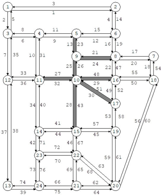
Figure 2. The topology of the Sioux Falls network.

There are 24 nodes and 76 links on the Sioux Falls network. The potential demands are assumed to be 500 for each OD pair listed in Table 1. For instance, between the OD pair (1,13), 500 travelers are willing to have trips from node 1 to node 13. On the network, the potential demands between the OD pairs, excluding those in Table 1, are zero.

Table 1. The OD pairs with potential demands.

OD Pair	OD Pair	OD Pair	OD Pair	OD Pair	OD Pair	OD Pair	OD Pair
(1,13)	(4,13)	(7,3)	(10,15)	(13,1)	(16,15)	(19,9)	(22,9)
(1,20)	(4,20)	(7,12)	(10,17)	(13,2)	(16,17)	(19,10)	(22,10)
(1,21)	(4,21)	(7,14)	(10,19)	(13,4)	(16,19)	(19,11)	(22,11)
(1,24)	(4,24)	(7,23)	(10,22)	(13,5)	(16,22)	(19,16)	(22,16)
(2,13)	(5,13)	(8,3)	(11,15)	(14,6)	(17,9)	(20,1)	(23,6)
(2,20)	(5,20)	(8,12)	(11,17)	(14,7)	(17,10)	(20,2)	(23,7)
(2,21)	(5,21)	(8,14)	(11,19)	(14,8)	(17,11)	(20,4)	(23,8)
(2,24)	(5,24)	(8,23)	(11,22)	(14,18)	(17,16)	(20,5)	(23,18)
(3,6)	(6,3)	(9,15)	(12,6)	(15,9)	(18,3)	(21,1)	(24,1)
(3,7)	(6,12)	(9,17)	(12,7)	(15,10)	(18,12)	(21,2)	(24,2)
(3,8)	(6,14)	(9,19)	(12,8)	(15,11)	(18,14)	(21,4)	(24,4)
(3,18)	(6,23)	(9,22)	(12,18)	(15,16)	(18,23)	(21,5)	(24,5)

The travel time function on link $a$ is calculated by the Bureau of Public Roads (BPR) function, which is proposed by the Bureau of Public Roads in the United States and is widely used to measure link travel time. The function is given by

$$t_a(x_a,C_a)=t_a^0[1+{\rho }_1{({\displaystyle \frac{x_a}{C_a}})}^{{\rho }_2}], a\in A$$

(32)

where ${\rho }_1$ and ${\rho }_2$ are parameters which are widely assumed to be 0.15 and 4, respectively. The free-flow travel time on link $a$ is shown in Table 2.

Table 2. The free-flow travel time of the network.

Link	${\mathit{t}}_{\mathit{a}}^0$ (min)	Link	${\mathit{t}}_{\mathit{a}}^0$ (min)	Link	${\mathit{t}}_{\mathit{a}}^0$ (min)	Link	${\mathit{t}}_{\mathit{a}}^0$ (min)	Link	${\mathit{t}}_{\mathit{a}}^0$ (min)
(1,2)	3	(6,8)	1	(11,4)	3	(15,22)	2	(20,19)	2
(1,3)	2	(7,8)	1.5	(11,10)	2.5	(16,8)	2.5	(20,21)	3
(2,1)	3	(7,18)	1	(11,12)	3	(16,10)	2.5	(20,22)	2.5
(2,6)	2.5	(8,6)	1	(11,14)	2	(16,17)	1	(21,20)	3
(3,1)	2	(8,7)	1.5	(12,3)	2	(16,18)	1.5	(21,22)	1
(3,4)	2	(8,9)	5	(12,11)	3	(17,10)	4	(21,24)	1.5
(3,12)	2	(8,16)	2.5	(12,13)	1.5	(17,16)	1	(22,15)	2
(4,3)	2	(9,5)	2.5	(13,12)	1.5	(17,19)	1	(22,20)	2.5
(4,5)	1	(9,8)	5	(13,24)	2	(18,7)	1	(22,21)	1
(4,11)	3	(9,10)	1.5	(14,11)	2	(18,16)	1.5	(22,23)	2
(5,4)	1	(10,9)	1.5	(14,15)	2.5	(18,20)	2	(23,14)	2
(5,6)	2	(10,11)	2.5	(14,23)	2	(19,15)	2	(23,22)	2
(5,9)	2.5	(10,15)	3	(15,10)	3	(19,17)	1	(23,24)	1
(6,2)	2.5	(10,16)	2.5	(15,14)	2.5	(19,20)	2	(24,13)	2
(6,5)	2	(10,17)	4	(15,19)	2	(20,18)	2	(24,21)	1.5
(24,23)	1

The headways of an HDV following another HDV on each link are shown in Table 3.

Table 3. The headways of HDVs on links.

Link	${\mathit{T}}_{\mathit{a}}^{\mathit{H}\mathit{H}}$ (s)	Link	${\mathit{T}}_{\mathit{a}}^{\mathit{H}\mathit{H}}$ (s)	Link	${\mathit{T}}_{\mathit{a}}^{\mathit{H}\mathit{H}}$ (s)	Link	${\mathit{T}}_{\mathit{a}}^{\mathit{H}\mathit{H}}$ (s)	Link	${\mathit{T}}_{\mathit{a}}^{\mathit{H}\mathit{H}}$ (s)
(1,2)	1.4	(6,8)	7.3	(11,4)	7.3	(15,22)	3.5	(20,19)	7.2
(1,3)	1.5	(7,8)	4.6	(11,10)	3.6	(16,8)	7.1	(20,21)	7.1
(2,1)	1.4	(7,18)	1.5	(11,12)	7.3	(16,10)	7	(20,22)	7.1
(2,6)	7.3	(8,6)	7.3	(11,14)	7.4	(16,17)	6.9	(21,20)	7.1
(3,1)	1.5	(8,7)	4.6	(12,3)	1.5	(16,18)	1.8	(21,22)	6.9
(3,4)	2.1	(8,9)	7.1	(12,11)	7.3	(17,10)	7.2	(21,24)	7.4
(3,12)	1.5	(8,16)	7.1	(12,13)	1.4	(17,16)	6.9	(22,15)	3.5
(4,3)	2.1	(9,5)	3.6	(13,12)	1.4	(17,19)	7.5	(22,20)	7.1
(4,5)	2	(9,8)	7.1	(13,24)	7.1	(18,7)	1.5	(22,21)	6.9
(4,11)	7.3	(9,10)	2.6	(14,11)	7.4	(18,16)	1.8	(22,23)	7.2
(5,4)	2	(10,9)	2.6	(14,15)	7	(18,20)	1.5	(23,14)	7.3
(5,6)	7.3	(10,11)	3.6	(14,23)	7.3	(19,15)	2.3	(23,22)	7.2
(5,9)	3.6	(10,15)	2.7	(15,10)	2.7	(19,17)	7.5	(23,24)	7.1
(6,2)	7.3	(10,16)	7	(15,14)	7	(19,20)	7.2	(24,13)	7.1
(6,5)	7.3	(10,17)	7.2	(15,19)	2.3	(20,18)	1.5	(24,21)	7.4
(24,23)	7.1

Other parameters are set as ${\lambda }_t=55$, $k=0.06$, $\theta =0.6$, $\gamma =0.1$, $\sigma =0.08$, ${\alpha }^{av}=0.7$, ${\alpha }^{HDV}=0.8$, ${\varphi }^{AV}=4.5$, ${\varphi }^{HDV}=3.5$, ${\varphi }^{Tr}=4$, ${\phi }^{Tr}=2.5$, $\tau =2.5$, $u_{av}=0.04$, and $u[t_a(x_a,C_a)]=u_{av}\cdot t_a(x_a,C_a)$. In reality, all the parameters can be obtained by approaches such as an RP investigation, the local literature investigation, etc. The parameters are obtained as an average reflection of the population, which are the input to our aggregated model. Therefore, the performances are aggregated as well. In this paper, we set the values as above to demonstrate the effects of the restriction scheme and verify the effectiveness of our model and algorithm. If an AV follows an AV, they are able to contact each other to obtain the operation information so that the headway $T_a^{AA}$ can be short enough. On the contrary, if an AV follows an HDV, they are probably not able to communicate with each other well, and the headway $T_a^{AH}$ is comparatively longer than that between AVs. However, it is still shorter than that between HDVs. Therefore, we assume $T_a^{AA}={\displaystyle \frac{1}{2}}{T}_a^H$ and $T_a^{AH}={\displaystyle \frac{2}{3}}{T}_a^H$.

We set the links (5,9), (9,5), (9,8), (8,9), (9,10), (10,9), (10,11), (11,10), (10,16), (16,10), (10,17), (17,10), (10,15), and (15,10) to construct a connected area for easy implementation. The performances of the traffic system with no restrictions, a proportion of 20%, and a proportion of 50% are listed in Table 4.

Table 4. The performances of the traffic system under the traffic restriction scheme.

The Proportion	Social Welfare	Total Generalized Travel Cost	The Demands
			AVs	HDVs	Transit	Total
0	567,280	167,177	5005	6744	18,469	30,218
20%	578,197	181,390	5492	7203	21,333	34,028
50%	583,992	175,535	5561	7079	21,853	34,493

The scheme with a proportion of 0% means there is no restriction scheme. From Table 4, we observe that without the traffic restriction scheme, both the social welfare and the total generalized travel cost are lowest, as well as the demands involving total demand and the respective demands of the three modes. Social welfare increases by 1.9% and 3% when the proportions are 20% and 50%, respectively, which shows the effectiveness of this scheme. Although the proportion is higher, the total demand is higher as well. This is because in the elastic demand case, a higher proportion of HDVs increases the capacity of relevant links, resulting in more trips. A higher proportion gives rise to increasing AVs and decreasing HDVs, which makes the system better organized and thereby brings a higher social welfare and a lower total generalized travel cost. From an economic perspective, the marginal cost of restricting an HDV may be lower than that of adding an AV. That is to say, if one HDV is restricted, more than one AV might emerge, which makes the system better.

Figure 3 depicts social welfare against various weights of an AV traveler and an HDV traveler weighting travel time. The results show that if AV travelers only care about the congestion level and HDV travelers only care about travel time, the social welfare achieves the maximum level. This is because the comfort of travelers in AVs is higher than those in HDVs. If the travelers only care about congestion level, the total cost may decrease. Note that social welfare exhibits a non-linear change with ${\alpha }^{av}$ and ${\alpha }^{HDV}$. It means there exists a ${\alpha }^{av}$/${\alpha }^{HDV}$ to minimize social welfare when ${\alpha }^{HDV}$/${\alpha }^{av}$ changes. In application, we are supposed to avoid the weight patterns which make social welfare the lowest.

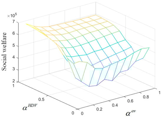
Figure 3. The weights versus the social welfare.

Figure 4 illustrates social welfares against the amortized costs of AVs and HDVs. It shows that the higher the amortized cost is, the higher the social welfare is, since a higher cost reduces the demand and thereby decreases traffic congestion. Note that if the amortized cost is extremely low, the social welfare is negative. This is because a lower amortized cost brings more auto travelers. In the presence of AVs, the travelers obtain higher utility if they choose Avs, while some of them would be restricted if they choose HDVs. In addition, more AVs enlarge the road capacity. Therefore, the auto demand further increases, resulting in excessive traffic congestion and negative social welfare. Another explanation from the economical perspective is that the marginal cost of the AV mode is lower than that of the HDV mode due to the utility of AV travelers and the restriction scheme for HDV travelers. Thus, more travelers prefer choosing to travel with AVs if they decide to travel, and the increment of vehicles is higher than that when in the conventional case in the absence of AVs. However, considering the acceptance of the public, the amortized cost cannot be too high. Therefore, moderate prices of AVs and HDVs are necessary.

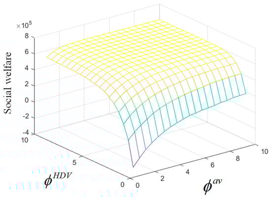
Figure 4. The amortized costs versus the social welfare.

Figure 5 shows the change in social welfares with respect to the fares of transit. In terms of the increasing fare, social welfare decreases as more travelers convert from transit to private vehicles. The change in social welfare with the fare of transit is non-monotonic due to the travel mode split and traffic assignment. If the fare is high, the social welfare becomes negative. The reason is similar to why the lower amortized costs give rise to negative social welfare. Therefore, for the purpose of increasing social welfare, the fare of transit is not supposed to be high.

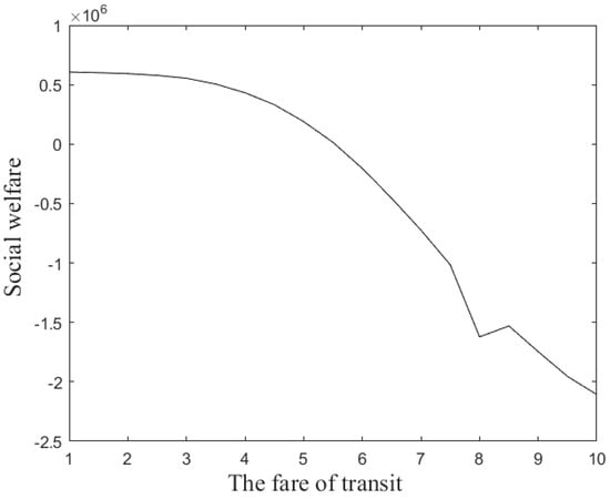
Figure 5. Social welfare versus the fare of transit.

Now, we change the headways to explore the system. Let $T_a^{AA}=AA\cdot T_a^R$ and $T_a^{AR}=AR\cdot T_a^R$, in which $AA$ and $AR$ are the parameters for an AV following another AV and an AV following an HDV, respectively. For reality, in this paper, we assume that the headway between AVs is smaller than that between an AV and an HDV. In other words, we assume $AA>AR$. Figure 6 portrays the change in social welfare when $AA$ and $AR$ change. It illustrates that smaller headways lead to higher social welfare, and social welfare is always positive if the headway between AVs is larger than that between AVs and HDVs. The gap between the two types of headways is not able to determine the social welfare, which may result from the demands of vehicles.

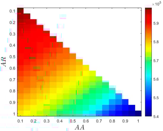
Figure 6. Social welfare versus various headways.

5. Conclusions

Taking the traffic system involving automated vehicles, human-driven vehicles, and transit into consideration, this paper proposes a traffic restriction scheme for human-driven vehicles. We construct a variational inequality model to describe the mode and route choice of travelers and propose an algorithm with the Gauss–Seidel algorithm to solve the model to capture the demand and flow patterns. Then, the model and algorithm are applied to a Sioux Falls network example. From the results, we have the main findings as follows:

• A traffic restriction scheme for human-driven vehicles is beneficial to traffic systems on increasing social welfare. A higher proportion of restriction schemes may bring higher demand, as well as higher social welfare in the elastic demand case, since more automated vehicles make the traffic system better organized. It can be taken as a traffic management demand scheme.
• Under the traffic restriction scheme for HDVs, there exists weighting coefficient patterns for weighting travel time and congestion levels that could minimize social welfare. In practice, this should be avoided. For example, intensifying the automation level of vehicles could alter the way automated vehicle users weight congestion level, thereby increasing social welfare.
• In the presence of the traffic restriction scheme for HDVs, a large value of exogenous monetary factors results in negative social welfare, as the marginal cost of automated vehicles is comparatively smaller, which gives rise to more travelers choosing private cars, thereby making roads more congested. Therefore, suitable monetary factors, e.g., the fare of transit and the price of vehicles, are necessary.
• In terms of the traffic restriction scheme for HDVs, shorter headways between automated vehicles, as well as between automated and human-driven vehicles, contribute to higher social welfare. However, social welfare is not solely determined by the difference in headways. Thus, advancements in automated driving technology should focus not only on connected automated vehicles but also on optimizing performance in mixed traffic flows.

All the results are with respect to the elements of the traffic system, such as the psychological level, transit ticket fare, amortized costs of owning vehicles, technologies, etc. Apparently, improvements on the elements give rise to better system performances. Nevertheless, the change in one element may lead to the change in some other elements. Therefore, in this paper, we indicate the direction of the improvements. The best improvements of all elements need to be specifically explored.

Besides the findings, some valuable extensions can be carried out for future directions.

• In this paper, the numerical results show that the scheme is beneficial to the system. Namely, it can be applied to a real case. It is worth collecting real data to analyze the system if needed. Some parameters such as the level of focusing on travel time and the utilities in a vehicle can be obtained by the RP investigation, while some other specific parameters such as link travel time and capacity, the transit ticket fare, etc., can be obtained by stated preference (SP) investigations. Full data are helpful to implement the scheme with the model and algorithm.
• In this study, we focus on three common modes within the mixed traffic system involving automated driving. However, other modes such as subways, bicycles, and taxis may also influence the system. It is therefore valuable to investigate a more comprehensive traffic system using a super network approach.
• We specifically examine the impacts of a given traffic restriction scheme on the traffic system. Future research could explore the optimal district configurations and proportional allocations for such schemes, as this holds significant research potential.
• Compared to traffic restriction schemes, pricing schemes have been more extensively studied. However, the marginal cost of automated vehicles remains unclear. A theoretical study on the marginal cost of automated vehicles from an economic perspective is a promising area for future research.

References

- Shi, F.; Yang, H.; Han, D.; Wang, X.; Yin, Y. Optimization method of alternate traffic restriction scheme based on elastic demand and mode choice behavior. Transp. Res. Part C Emerg. Technol. 2014, 39, 36–52. [Google Scholar] [CrossRef]
- Han, D.; Yang, H.; Wang, X. Efficiency of the plate-number-based traffic rationing in general networks. Transp. Res. Part E Logist. Transp. Rev. 2010, 46, 1095–1110. [Google Scholar] [CrossRef]
- Wang, X.; Yang, H.; Han, D. Traffic rationing and short-term and long-term equilibrium. Transp. Res. Rec. 2010, 2196, 131–141. [Google Scholar] [CrossRef]
- Chen, D.; Sun, Y.; Yang, Z. Optimization of the travel ban scheme of cars based on the spatial distribution of the last digit of license plates. Transp. Policy 2020, 94, 43–53. [Google Scholar] [CrossRef]
- Daganzo, C.F.; Garcia, R.C. A Pareto improving strategy for the time-dependent morning commute problem. Transp. Sci. 2000, 34, 303–311. [Google Scholar] [CrossRef]
- Nakamura, K.; Kockelman, K.M. Congestion pricing and roadspace rationing: An application to the San Francisco Bay Bridge corridor. Transp. Res. Part A Policy Pract. 2002, 36, 403–417. [Google Scholar] [CrossRef][Green Version]
- Song, Z.; Yin, Y.; Lawphongpanich, S. A Pareto-improving hybrid policy for transportation networks. J. Adv. Transp. 2014, 48, 272–286. [Google Scholar] [CrossRef]
- Xu, G.; Chen, Y.; Liu, W. Joint optimisation of park-and-ride facility locations and alternate traffic restriction scheme under equilibrium flows. Transp. A Transp. Sci. 2023, 19, 2077468. [Google Scholar] [CrossRef]
- Nie, Y. Why is license plate rationing not a good transport policy? Transp. A Transp. Sci. 2017, 13, 1–23. [Google Scholar] [CrossRef]
- Yao, Z.; Jia, Y.; Li, Y.; Jin, P.; Hou, Y.; Huang, H.J. Analysis of the impact of maximum platoon size of CAVs on mixed traffic flow: An analytical and simulation method. Transp. Res. Part C Emerg. Technol. 2023, 147, 103989. [Google Scholar] [CrossRef]
- Ghiasi, A.; Hussain, O.; Qian, X.; Li, X. A mixed traffic capacity analysis and lane management model for connected automated vehicles: A Markov chain method. Transp. Res. Part B Methodol. 2017, 106, 266–292. [Google Scholar] [CrossRef]
- Sun, J.; Zheng, Z.; Sun, J. The relationship between car following string instability and traffic oscillations in finite-sized platoons and its use in easing congestion via connected and automated vehicles with IDM based controller. Transp. Res. Part B Methodol. 2020, 142, 58–83. [Google Scholar] [CrossRef]
- Lin, W.; Zheng, Z.; Sun, J.; Wang, Y.; Ma, L. Rhythmic control of automated traffic—Part II: Grid network rhythm and online routing. Transp. Sci. 2021, 55, 988–1009. [Google Scholar] [CrossRef]
- Qin, Y.; Wang, H.; Ran, B. Impacts of cooperative adaptive cruise control platoons on emissions under traffic oscillation. J. Intell. Transp. Syst. 2021, 25, 376–383. [Google Scholar] [CrossRef]
- Kaddoura, I.; Bischoff, J.; Nagel, K. Towards welfare optimal operation of innovative mobility concepts: External cost pricing in a world of shared autonomous vehicles. Transp. Res. Part A Policy Pract. 2020, 136, 48–63. [Google Scholar] [CrossRef]
- Simoni, M.D.; Kockelman, K.M.; Gurumurthy, K.M.; Bischoff, J. Congestion pricing in a world of self-driving vehicles: An analysis of different strategies in alternative future scenarios. Transp. Res. Part C Emerg. Technol. 2019, 98, 167–185. [Google Scholar] [CrossRef]
- Sharon, G.; Stone, P.; Boyles, S.D.; Unnikrishnan, A. Network-wide adaptive tolling for connected and automated vehicles. Transp. Res. Part C Emerg. Technol. 2017, 84, 142–157. [Google Scholar] [CrossRef]
- Gurumurthy, K.M.; Kockelman, K.M.; Simoni, M.D. Benefits and costs of ride-sharing in shared automated vehicles across Austin, Texas: Opportunities for congestion pricing. Transp. Res. Rec. 2019, 2673, 548–556. [Google Scholar] [CrossRef]
- Ye, Y.; Wang, H. Optimal design of transportation networks with automated vehicle links and congestion pricing. J. Adv. Transp. 2018, 2018, 3435720. [Google Scholar] [CrossRef]
- Delle Site, P. Pricing of connected and autonomous vehicles in mixed-traffic networks. Transp. Res. Rec. 2021, 2675, 178–192. [Google Scholar] [CrossRef]
- Liu, A.; Liu, Z.; He, Z. Joint optimal pricing strategy of shared autonomous vehicles and road congestion pricing: A regional accessibility perspective. Cities 2024, 146, 104742. [Google Scholar] [CrossRef]
- Mansourianfar, M.H.; Hassan, A.H.; Abou-Zeid, M.; Sadek, A. Joint routing and pricing control in congested mixed autonomy networks. Transp. Res. Part C Emerg. Technol. 2021, 131, 103338. [Google Scholar] [CrossRef]
- Tscharaktschiew, S.; Evangelinos, C. Pigouvian road congestion pricing under autonomous driving mode choice. Transp. Res. Part C Emerg. Technol. 2019, 101, 79–95. [Google Scholar] [CrossRef]
- Francisco, F.; Pang, J.-S. Finite-Dimensional Variational Inequalities and Complementarity Problems; Springer: New York, NY, USA, 2003. [Google Scholar]
Disclaimer/Publisher’s Note: The statements, opinions and data contained in all publications are solely those of the individual author(s) and contributor(s) and not of MDPI and/or the editor(s). MDPI and/or the editor(s) disclaim responsibility for any injury to people or property resulting from any ideas, methods, instructions or products referred to in the content. |
© 2024 by the authors. Licensee MDPI, Basel, Switzerland. This article is an open access article distributed under the terms and conditions of the Creative Commons Attribution (CC BY) license (https://creativecommons.org/licenses/by/4.0/).